KMT-2018-BLG-1990Lb: A Nearby Jovian Planet From A Low-Cadence Microlensing Field

Abstract

We report the discovery and characterization of KMT-2018-BLG-1990Lb, a Jovian planet $(m_{p}=0.57_{-0.25}^{+0.79}\,M_{J})$ orbiting a late M dwarf $(M=0.14_{-0.06}^{+0.20}\,M_{\odot})$, at a distance $(D_{L}=1.23_{-0.43}^{+1.06}\,{\rm kpc})$, and projected at $2.6\pm 0.6$ times the snow line distance, i.e., $a_{\rm snow}\equiv 2.7\,{\rm au}(M/M_{\odot})$, This is the second Jovian planet discovered by KMTNet in its low cadence ($0.4\,{\rm hr}^{-1}$) fields, demonstrating that this population will be well characterized based on survey-only microlensing data.

1 Introduction

The Korea Microlensing Telescope Network (KMTNet, Kim et al. 2016) monitors about 97 deg² toward the Galactic bulge from three 1.6m telescopes that are equipped with 4 deg² cameras, in Chile (KMTC), South Africa (KMTS), and Australia (KMTA). Its primary goal is to find exoplanets via the anomalies that these generate in microlensing events (Mao & Paczyński, 1991).

For many years, (beginning with the second microlensing planet OGLE-2005-BLG-071Lb, Udalski et al. 2005), most microlensing planets were discovered by intensive follow-up observations of microlensing events that were alerted by wide-field surveys. Gould & Loeb (1992) had advocated such a strategy because microlensing events, which have typical Einstein timescales $t_{\rm E}\sim 20\,$days, can be discovered even in very low-cadence surveys $\Gamma\lesssim 1\,{\rm day}^{-1}$, whereas the fleeting appearance of planetary anomalies requires much higher cadence to detect and, more critically, to reasonably characterize the planet. In their scheme, the microlensing surveys could cover very broad areas from even a single site, while narrow-angle follow-up observations could be carried out around the clock at much higher cadence on a handful of favorable targets.

By continuously monitoring a broad area at relatively high-cadence from its three sites, KMTNet aimed to simultaneously find microlensing events and find and characterize the planetary anomalies within them, without any followup observations (and hence without the necessity of microlensing alerts). In 2015, its first (commissioning) year of observation, KMTNet narrowly focused on this strategy (Kim et al., 2018a). It observed only four fields, allowing a very high cadence of $\Gamma=6\,{\rm hr}^{-1}$, which as we will discuss immediately below, was sufficient to detect planets down to about one Earth mass.

However, beginning in 2016, KMTNet developed a radically different strategy, with a range of cadences $\Gamma=(4,1,0.4,0.2)\,{\rm hr}^{-1}$ covering areas of (12,29,44,12) deg², respectively. See Figure 12 of Kim et al. (2018a). This change was motivated by a variety of goals, including support for Spitzer microlensing (Gould et al., 2013, 2014, 2015a, 2015b, 2016, 2018), which is an intrinsically wide-field experiment. However, a major goal was simply to find and characterize more planets over a much broader area.

The half-duration of a planetary perturbation is roughly the planetary Einstein time

$$t_{{\rm E},p}={\theta_{{\rm E},p}\over\mu_{\rm rel}}\simeq 1.25\,{\rm hr}\biggl{(}{m_{p}\over M_{\oplus}}\biggr{)}^{1/2}\biggl{(}{\pi_{\rm rel}\over 0.02\,{\rm mas}}\biggr{)}^{1/2}\biggl{(}{\mu_{\rm rel}\over 5\,{\rm mas}\,{\rm yr}^{-1}}\biggr{)}^{-1},$$ (1)

where

$$\theta_{{\rm E},p}\equiv\sqrt{q\over 1+q}\theta_{\rm E};\qquad\theta_{\rm E}\equiv\sqrt{\kappa M\pi_{\rm rel}};\qquad\kappa\equiv{4G\over c^{2}{\rm au}}\simeq 8.14\,{{\rm mas}\over M_{\odot}},$$ (2)

$q\equiv m_{p}/M$ is the planet-host mass ratio, $\theta_{\rm E}$ is the Einstein radius, and $\pi_{\rm rel}$ and ${\mbox{\boldmath$\mu$}}_{\rm rel}$ are, respectively, the lens-source relative parallax and proper motion. Thus, assuming that about 10 data points are needed over the full anomaly, the adopted cadences of $\Gamma=(4,1,0.4,0.2)\,{\rm hr}^{-1}$ should be sufficient to detect planets of mass $m_{p}\sim(1,16,100,400)\,M_{\oplus}$, corresponding to “Earth”, “Neptune”, “Saturn” and “Jupiter” mass planets. See also Kim et al. (2018d) and Figure 14 from Henderson et al. (2014). In effect, the revised strategy sacrificed sensitivity to Earth-mass planets over 4 deg² in order to expand the total area by a factor 6, including a 2.5 fold increase in the area sensitive to Neptunes.

Here we report on KMT-2018-BLG-1990Lb, a Jovian mass planet lying in field BLG38, which is monitored by KMTNet at $\Gamma=0.4\,{\rm hr}^{-1}$ and at a position that was not monitored by other surveys. It is the second KMT-only Jovian planet from a field with this cadence, the first being KMT-2016-BLG-1397Lb from BLG31 (Zang et al., 2018). As such, it demonstrates the viability of a wide-field survey for gas giant planets in accord with the KMTNet strategy.

2 Observations

KMT-2018-BLG-1990 is at (RA,Dec) = (17:53:44.49,$-22$:09:09.14), corresponding to $(l,b)=(6.77,1.91)$, i.e., well out along the near side of the Galactic bar. As mentioned in Section 1, it lies in KMTNet field BLG38, which has a nominal cadence of $\Gamma=0.4\,{\rm hr}^{-1}$. However, from the start of the season through 25 June 2018, KMTNet followed a modified survey strategy in which BLG38 continued to be observed at $\Gamma=0.4\,{\rm hr}^{-1}$ from KMTC, but was observed at $\Gamma=0.3\,{\rm hr}^{-1}$ from KMTS and KMTA. This period contained virtually the whole of the event.

The great majority of observations were carried out in the $I$ band, but about 9% were in $V$ band. The primary purpose of the latter was to determine the source color. All reductions for this analysis were conducted using variants of image subtraction (Alard & Lupton, 1998). In particular, a variant of the Woźniak (2000) difference image analysis (DIA) code was used for pipeline reductions of the 500 million light curves that were searched for microlensing events. Then pySIS (Albrow et al., 2009) pipeline re-reductions were carried out to further check whether the event is indeed microlensing, and finally tender loving care (TLC) pySIS re-reductions were used to derive parameters. A separate package, pyDIA (Albrow, 2017), was used to construct the color-magnitude diagram (CMD).

The event was discovered by applying the KMTNet event-finder algorithm (Kim et al., 2018a) to the 2018 DIA light curves. Very briefly, a machine review of these light curves chose this event (among 100,130 candidates) for human review. The DIA light curve (which can be accessed at http://kmtnet.kasi.re.kr/ulens/) is easily and securely identified as microlensing, but actually displays no clear signature of an anomaly. The anomaly was discovered after running pipeline pySIS on the BLG38 candidates in order to conduct a final review of these candidates. The pipeline pySIS reduction (also accessible at http://kmtnet.kasi.re.kr/ulens/) shows a double-horned anomaly, characteristic of a planetary or binary caustic crossing, which was immediately investigated and revealed to be planetary. By chance, this was the first 2018 event-finder microlensing-event candidate that was examined manually.

3 Analysis

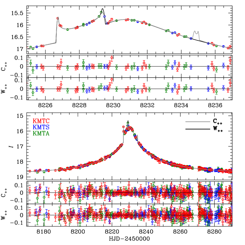
Figure 1: Light curve of KMT-2018-BLG-1990 with data from the three KMTNet observatories. The curves show the $C_{++}$ and $W_{++}$ models from Tables 2 and 3, but the other six degenerate models in these Tables look extremely similar.

Figure 1 shows the KMT-2018-BLG-1990 data together with the best-fit model. The light curve shows a roughly 65 hr anomaly just before the peak of an otherwise normal Paczyński (1986) point-lens light curve. According to the naive scaling given in Section 1, this should correspond to an $m_{p}\sim 10^{3}\,M_{\oplus}$ companion. It should be noted that a broadly similar morphology can be generated when a source transits the relatively small “Chang-Refsdal” caustic of a wide ($s\gg 1$) or close ($s\ll 1$) binary with comparable-mass components, followed by a cusp approach. In this case, however, one would expect that the peak would be offset from the center of the light curve as defined by the wings. Nevertheless, this example serves as a caution that a thorough examination of parameter space should be undertaken, even when the caustic geometry appears “obvious”.

We proceed by a standard search for solutions defined by seven non-linear parameters: $(t_{0},u_{0},t_{\rm E},s,q,\alpha,\rho)$. The first three are the Paczyński (1986) parameters of the underlying point-lens events: (time of closest approach, impact parameter in units of $\theta_{\rm E}$, Einstein timescale $t_{\rm E}=\theta_{\rm E}/\mu_{\rm rel}$). The next three define the binary geometry: (separation in units of $\theta_{\rm E}$, mass ratio, orientation of binary axis relative to ${\mbox{\boldmath$\mu$}}_{\rm rel}$). The last, $\rho=\theta_{*}/\theta_{\rm E}$, is the source radius normalized to the Einstein radius. In addition, there are two flux parameters for each observatory $i$, i.e., the source flux $f_{s,i}$ and the blend flux $f_{b,i}$, so that the model flux is given by $F_{i}(t)=f_{s,i}A(t)+f_{b,i}$, where $A(t)$ is the model magnification.

We first conduct a grid search, holding $(s,q)$ fixed on a grid of values and allowing all other parameters to vary in a Monte Carlo Markov chain (MCMC). For the three Paczyński (1986) parameters, we seed the chains with the results from a point-lens fit (with the anomaly removed). For $\alpha$, we seed with six values taken uniformly around the unit circle. Finally, we seed the normalized source radius with $\rho=10^{-3}$. The flux parameters are determined by a linear fit to the data for each trial model. We find that there are two solutions, which are related by the so-called close-wide degeneracy, which approximately takes $s\rightarrow s^{-1}$. In fact, this degeneracy was originally derived in the limits $s\gg 1$ or $s\ll 1$ (Griest & Safizadeh, 1998), but sometimes holds when $s\sim 1$ as well.

We then conduct a refined search on each of these two solutions by allowing all seven geometric parameters to vary in the MCMC. The results are shown in Table 1. Note that, in contrast to the limiting cases from which this degeneracy is derived, the $s\rightarrow s^{-1}$ transformation does not preserve the value of $q$. Instead, $q(s<1)\sim 3.7\times 10^{-3}$, while $q(s>1)\sim 6.2\times 10^{-3}$.

3.1 Microlens Parallax: ${\mbox{\boldmath$\pi$}}_{\rm E}$

Next, we consider the microlens parallax effect. A combination of two facts strongly suggests that this effect will be measurable, or at least strongly constrained. First, the timescale is relatively long, $t_{\rm E}\sim 45\,$days, implying that Earth’s velocity projected on the sky changes by $\Delta v\sim 35\,{\rm km}\,{\rm s}^{-1}$ during the $\sim 2t_{\rm E}$ time interval when the source is significantly magnified.

Second, as we will show in Section 4.1, $\theta_{*}\sim 1.2\,\mu{\rm as}$. Combining this with the measured value of $\rho\sim 1.2\times 10^{-3}$ implies $\theta_{\rm E}=\theta_{*}/\rho\simeq 1.0\,{\rm mas}$. The microlens parallax vector is given by

$${\mbox{\boldmath$\pi$}}_{\rm E}\equiv{\pi_{\rm rel}\over\theta_{\rm E}}\,{{\mbox{\boldmath$\mu$}}_{\rm rel}\over\mu_{\rm rel}},$$ (3)

which immediately yields (Gould, 1992, 2000),

$$\pi_{\rm rel}=\theta_{\rm E}\pi_{\rm E};\qquad M={\theta_{\rm E}\over\kappa\pi_{\rm E}}.$$ (4)

Hence, $\theta_{\rm E}\simeq 1.0\,{\rm mas}$ implies $M\lesssim 1\,M_{\odot}$ and $\pi_{\rm rel}\lesssim 0.13\,{\rm mas}$. Otherwise the lens would be easily visible in the blended light. Then, from the limit on $\pi_{\rm rel}$, we can also place limits on the amplitude of the lens-source projected velocity $\tilde{\bf v}\equiv({\rm au}/t_{\rm E}){\mbox{\boldmath$\pi$}}_{\rm E}/\pi_{\rm E}^{2}$,

$$\tilde{v}={{\rm au}\over t_{\rm E}\pi_{\rm E}}={{\rm au}\over\pi_{\rm rel}}\,{\theta_{\rm E}\over t_{\rm E}}\lesssim 290\,{\rm km}\,{\rm s}^{-1}.$$ (5)

That is, during the event, the lens-source motion as observed from Earth changes fractionally by at least $\Delta v/\tilde{v}\gtrsim 12\%$. We introduce two additional parameters $(\pi_{{\rm E},N},\pi_{{\rm E},E})$, which are the components of ${\mbox{\boldmath$\pi$}}_{\rm E}$ in the Equatorial coordinate system. Because the effects of Earth’s orbital motion can be correlated with the effects of lens orbital motion, it is essential to simultaneously consider the latter, which we parameterize by $(ds/dt,d\alpha/dt)$, the instantaneous changes in the separation and orientation of the two components at $t_{0}$. In fact, we find that the orbital parameters are only weakly constrained. We therefore restrict the MCMC trials by the condition $\beta<0.8$, where $\beta$ is the ratio of projected kinetic to potential energy

$$\beta=\bigg{|}{\rm KE\over PE}\bigg{|}_{\perp}={\kappa M_{\odot}{\rm yr}^{2}\over 8\pi^{2}}{\pi_{\rm E}\over\theta_{\rm E}}\gamma^{2}\biggl{(}{s\over\pi_{\rm E}+\pi_{s}/\theta_{\rm E}}\biggr{)}^{3};\qquad{\mbox{\boldmath$\gamma$}}\equiv\biggl{(}{ds/dt\over s},{d\alpha\over dt}\biggr{)},$$ (6)

where we adopt $\pi_{s}=0.14\,{\rm mas}$ for the source parallax.

As usual, we must consider the “ecliptic degeneracy”, which takes $(u_{0},\alpha,\pi_{{\rm E},\perp},d\alpha/dt)\rightarrow-(u_{0},\alpha,\pi_{{\rm E},\perp},d\alpha/dt)$ (Skowron et al., 2011), where $\pi_{{\rm E},\perp}$ is the component of ${\mbox{\boldmath$\pi$}}_{\rm E}$ that is perpendicular to the direction of Earth’s acceleration (projected on the sky) at $t_{0}$. Indeed, because the event is very close to the ecliptic, $\beta_{\rm ecliptic}=+1.3^{\circ}$, we expect this degeneracy to be very severe: it is exact in the limit $\beta_{\rm ecliptic}\rightarrow 0$.

We find that for each of the four near-degenerate combinations $[(s<1),(s>1)]\times[(u_{0}<0),(u_{0}>0)]$, there are two local minima, which are characterized by different values of $\pi_{{\rm E},N}$. Such a discrete degeneracy is predicted by the “jerk-parallax degeneracy” (Gould, 2004), according to which

$$\pi_{{\rm E},\perp}^{\prime}=-(\pi_{{\rm E},\perp}+\pi_{j,\perp})$$ (7)

where $\pi_{j,\perp}$ is the “jerk parallax”. From Equations (8) and (9) of Park et al. (2004), which make a number of simplifying approximations,

$$\pi_{j,\perp}=-{4\over 3}\,{{\rm yr}\over 2\pi t_{\rm E}}\,{\sin\beta_{\rm ecliptic}\over(\cos^{2}\psi\sin^{2}\beta_{\rm ecliptic}+\sin^{2}\psi)^{3/2}}\rightarrow-0.05,$$ (8)

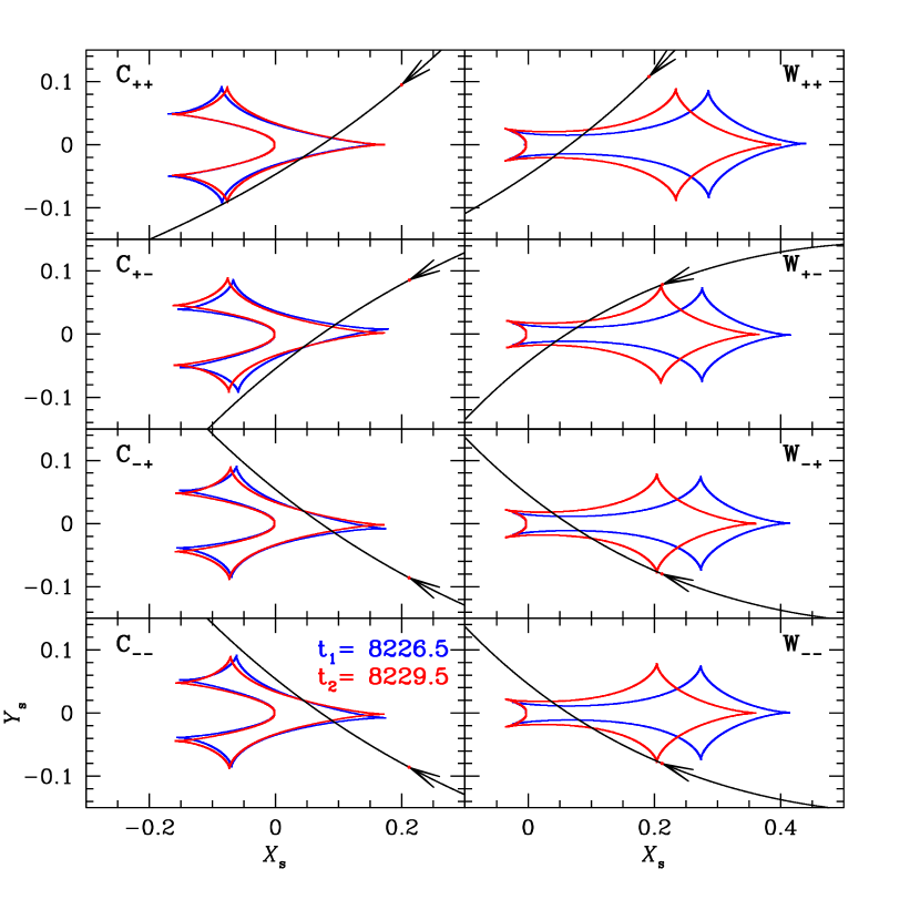
Figure 2: Caustic geometries for each of the eight solutions shown in Tables 2 and 3. The red and blue closed curves show the caustics at the two designated epochs, while the black curves show the source trajectory relative to these structures.

where $\psi\rightarrow 57^{\circ}$ is the ecliptic-latitude offset between the anti-Sun and the event at $t_{0}$. Because Earth’s projected acceleration is within $0.2^{\circ}$ of due west at the peak of the event, $\pi_{{\rm E},\perp}\simeq\pi_{{\rm E},N}$. (Note that because the $(\pi_{{\rm E},\parallel},\pi_{{\rm E},\perp})$ system is right-handed, $\pi_{{\rm E},\perp}\sim\pi_{{\rm E},N}$ for the first several months of the microlensing season and $\pi_{{\rm E},\perp}\sim-\pi_{{\rm E},N}$ during the last several months. See, e.g., Figure 3 from Park et al. 2004.) Therefore, from the fact that one $(s<0,u_{0}<0)$ solution has $\pi_{{\rm E},N}=1.39$, the jerk-parallax formalism predicts that the other should have $\pi_{{\rm E},N}^{\prime}=-(\pi_{{\rm E},N}+\pi_{j,\perp})=-1.34$. The actual value ($-1.12$) is in reasonable agreement, given the error bars. The situation is qualitatively similar for the other three pairs of solutions. We note that the jerk-parallax degeneracy has never previously been investigated in the context of planetary microlensing events. The caustic geometries of these eight solutions are shown in Figure 2, and their parameters are given in Tables 2 and 3.

The first point to note about these eight solutions is that they have similar $\chi^{2}$, which means that all must be considered as viable. To facilitate the further discussion of these eight solutions, we label them by, $C_{\pm\pm}$ or $W_{\pm\pm}$. The letter stands for “close” or “wide” (for $s<1$ or $s>1$), while the two subscripts refer to the signs of $u_{0}$ and $\pi_{{\rm E},N}$, respectively.

Second, we note that six of the eight solutions have very comparable values of $q$: the close solutions have $q\simeq 3.6\times 10^{-3}$, while the $W_{+-}$ and $W_{-+}$ solutions have $q\simeq 4.2\times 10^{-3}$. On the other hand, the solutions $W_{++}$ and $W_{--}$ have significantly higher $q\simeq 5.6\times 10^{-3}$. Note that these two solutions have $\Delta\chi^{2}\sim 4$ relative to the best solution, and therefore this higher mass ratio will end up getting less weight in the final parameter estimates.

Third, all eight solutions have qualitatively comparable values of $\pi_{\rm E}$. That is, in all cases $|\pi_{{\rm E},N}|\gg|\pi_{{\rm E},E}|$ and in all cases $|\pi_{{\rm E},N}|$ have comparable values. These facts together mean that $\pi_{\rm E}\simeq|\pi_{{\rm E},N}|$ are similar for all four solutions. Because the errors on $\pi_{{\rm E},N}$ are relatively large, it is important to assess whether these solutions are well localized. We display the ${\mbox{\boldmath$\pi$}}_{\rm E}$ distributions in Figure 3, which shows that they are indeed well-localized at the two-sigma level, but less so at the three-sigma level.

Fourth, we note that the remaining microlensing parameters are also comparable between solutions, with the exception of the orbital parameters. However, these are basically just nuisance parameters, which are very poorly constrained and are included only to avoid biasing the parallax parameters.

4 Physical Parameters

Whenever $\theta_{\rm E}$ and $\pi_{\rm E}$ are well measured, one can always determine the relative parallax $\pi_{\rm rel}$ and the lens mass $M$ from Equation (4), and so the lens distance $D_{L}={\rm au}/(\theta_{\rm E}\pi_{\rm E}+\pi_{s})$. In the present case, there are eight different solutions, but the best fit values for each of these will lead to fairly similar values $M\sim 0.09\,M_{\odot}$, $D_{L}\sim 0.8\,{\rm kpc}$. This distance is unusually small because the phase space, which grows quadratically with distance, generally favors more distant lenses. Smaller values of the microlens parallax would, by Equation (4), give larger distances. Therefore, symmetric errors in $\pi_{\rm E}$ (which is essentially equal to $|\pi_{{\rm E},N}|$ in the present case) should give rise to an asymmetric distribution in inferred distance around the value derived from the best fit. When the errors in $\pi_{\rm E}$ are small, this effect is likewise small and can be ignored. However, in the present case, both the variation in $\pi_{\rm E}$ between solutions and the statistical errors within solutions are fairly large. Hence, this effect must be accounted for. We will address this in Section 4.3. Before doing so, however, we must first evaluate $\theta_{*}$ (Section 4.1) and investigate the proper-motion distribution of the microlensed source (Section 4.2).

4.1 CMD

The first step toward estimating physical parameters is to measure the source position on the CMD relative to the centroid of the red clump, which then permits one to estimate $\theta_{*}$ and thus $\theta_{\rm E}=\theta_{*}/\rho$. We first note that while the source color estimate does not depend on the microlensing model (and can often be derived by regression of $V$ on $I$ flux, without any model), the source magnitude does depend on the model. Therefore, for simplicity, we will explicitly derive results for the $C_{-+}$ model and then present scaling relations for the rest.

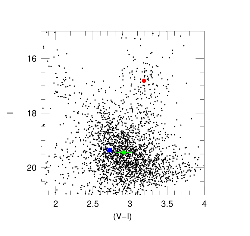
Figure 4: Color-Magnitude Diagram (CMD) of stars within a $2^{\prime}$ square box centered on KMT-2018-BLG-1990. The position of the microlensed source, the blended light and the centroid of the red clump are shown as blue, green, and red circles, respectively. The values shown here are taken from the $C_{-+}$ solution, but the other solutions would be virtually indistinguishable on this plot.

The CMD is shown in Figure 4, with the source and blend positions marked. The clump centroid is at $[(V-I),I]_{\rm cl}=(3.19,16.82)\pm(0.02,0.08)$, whereas the source is at $[(V-I),I]_{s}=(2.73,19.36)\pm(0.02,0.05)$, The errors in the clump position are due to centroiding. The source color and error are derived from regression without reference to any model. The source magnitude error is set to 0.05 as representative of all solutions, which have very similar error bars. Hence, the offset from the clump is $\Delta[(V-I),I]=(-0.46,2.54)\pm(0.03,0.10)$. We adopt $[(V-I),I]_{\rm cl,0}=(1.06,14.25)$ from Bensby et al. (2013) and Nataf et al. (2013), and so derive $[(V-I),I]_{s,0}=(0.60,16.79)\pm(0.03,0.10)$. We have not included any error in the de-reddened position of the clump, but rather add an overall 5% error to $\theta_{*}$ due to all aspects of the method. We convert from $V/I$ to $V/K$ using the color-color relations of Bessell & Brett (1988), and then use the color/surface-brightness relation of Kervella et al. (2004) to derive

$$\theta_{*}=1.23\pm 0.09\ \mu{\rm as};\qquad\theta_{\rm E}=0.88\pm 0.11\ {\rm mas};\qquad\mu_{\rm rel}=7.1\pm 0.9\ {\rm mas}\,{\rm yr}^{-1},$$ (9)

where we have used $\rho=1.39\pm 0.16$ from the $C_{-+}$ solution, and where we have taken account of the anti-correlation between $f_{s}$ and $\rho$. For other solutions, one can simply scale $\theta_{*}/\theta_{*,C,-,+}=\sqrt{f_{s}/0.347}$ and $\theta_{\rm E}/\theta_{{\rm E},C,-,+}=\sqrt{f_{s}/0.347}/(\rho/1.39\times 10^{-3})$.

4.2 Source Proper Motion

The source proper motion ${\mbox{\boldmath$\mu$}}_{s}$ is one of many inputs into a Bayesian estimate of the lens properties. For relatively bright sources, it is often possible to measure their proper motions, either from Gaia or from ground-based data. When this is not possible, one usually adopts an assumed distribution of source proper motions derived from a Galactic model. In the present case, the source is too faint and blended to measure its proper motion from ground data. In any case, the KMT time baseline would be too short for an accurate measurement. Moreover, the source does not appear in Gaia.

However, we can still use Gaia to measure the proper-motion distribution of “bulge” (really, “bar”) stars, of which the microlensed source is very likely a member. We examine a Gaia CMD and on this basis select the 82 stars within $1^{\prime}$ and satisfying $G<18.6$ and $B_{p}-R_{p}>2.6$. We eliminate one outlier and derive (in the Sun frame)

$$\langle{\mbox{\boldmath$\mu$}}_{\rm bar}(l,b)\rangle=(-5.4,0.1)\pm(0.3,0.2)\,{\rm mas}\,{\rm yr}^{-1};\quad\sigma({\mbox{\boldmath$\mu$}}_{\rm bar})=(2.9,2.2)\pm(0.2,0.2)\,{\rm mas}\,{\rm yr}^{-1}$$ (10)

4.3 Bayesian Analysis

Normally, one does not apply a Bayesian analysis when $\theta_{\rm E}$ and ${\mbox{\boldmath$\pi$}}_{\rm E}$ are relatively well measured. Rather one would simply combine these measurements using Equation (4) to obtain $M$ and $\pi_{\rm rel}$ (and so $D_{L}$), and propagate the errors in the measured quantities to the physical quantities. However, we argued at the beginning of Section 4 that in the present case, a full Bayesian analysis was justified. Stating the argument differently, if the errors are “small”, then the frequentist and Bayesian approaches will yield nearly identical results, so there is no point employing the more cumbersome Bayesian formalism. And whether the errors can be considered “small” depends on the product of their absolute size and the gradient of the priors. In the present case, the errors should be considered “large” given the steepness of the gradient.

We draw random events from a Galactic model, as described in detail by Jung et al. (2018). The only exception is that we draw the source proper motions from a Gaussian distribution with the parameters that were derived from Gaia data in Section 4.2.

Each of the eight solutions is fed exactly the same ensemble of $10^{8}$ simulated events. For each solution, each simulated event is given a weight equal to the likelihood of its four inferred parameters $(t_{\rm E},\theta_{\rm E},\pi_{{\rm E},N},\pi_{{\rm E},E})$ given the error distributions of these quantities derived from the MCMC for that solution. Finally, we weight by $\exp(-\Delta\chi^{2}_{k}/2)$, where $\Delta\chi^{2}_{k}$ is the difference in $\chi^{2}$ between the $k$th solution and the best fit.

Hence, the $i$th simulated event in the $k$th solution is given a weight of

$$w_{i,k}={\cal L}_{i,k}(t_{\rm E}){\cal L}_{i,k}(\theta_{\rm E}){\cal L}_{i,k}({\mbox{\boldmath$\pi$}}_{\rm E})\exp(-\Delta\chi^{2}_{k}/2)$$ (11)

where

$${\cal L}_{i,k}(X)={\exp[-(X_{i}-X_{k})^{2}/2\sigma_{X_{k}}^{2}]\over 2\pi\sigma_{X_{k}}},\qquad X=t_{\rm E}\ {\rm or}\ X=\theta_{\rm E},$$ (12)

$${\cal L}_{i,k}({\mbox{\boldmath$\pi$}}_{\rm E})={\exp[-\sum_{m,n=1}^{2}b^{k}_{m,n}(\pi_{{\rm E},m,i}-\pi_{{\rm E},m,k})(\pi_{{\rm E},n,i}-\pi_{{\rm E},n,k})/2]\over(2\pi)^{2}/\sqrt{{\rm det}\,b^{k}}},$$ (13)

$b^{k}_{m,n}$ is the inverse covariance matrix of the ${\mbox{\boldmath$\pi$}}_{\rm E}$ parallax vector in the $k$-th solution, and $(m,n)$ are dummy variables ranging over $(N,E)$.

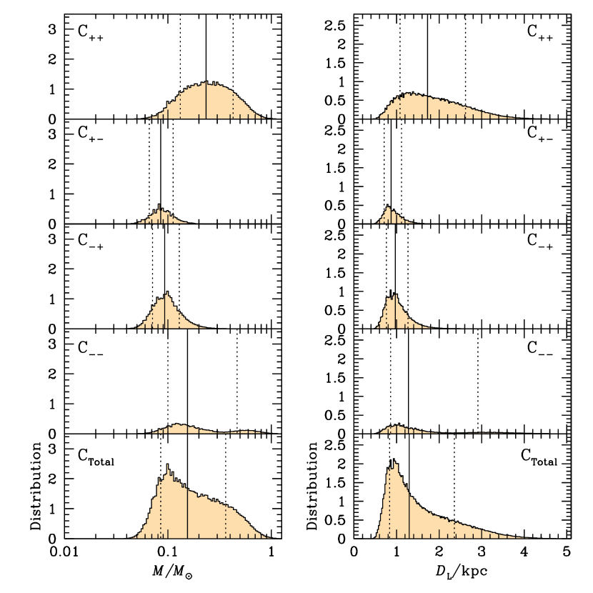
Figure 5: Histogram of the Bayesian posteriors of the lens mass and distance for each of the four of close solutions (top four rows) and the sum of all four solutions (bottom row). The total area in each histogram is proportional to the product of the weight derived from Bayesian analysis and $\exp(-\Delta\chi^{2}/2)$ of the solution. The $C_{++}$ solution ($u_{0}>0$, $\pi_{{\rm E},N}>0$) dominates primarily because it is compatible with more distant lenses, which are more numerous in the Galactic model.

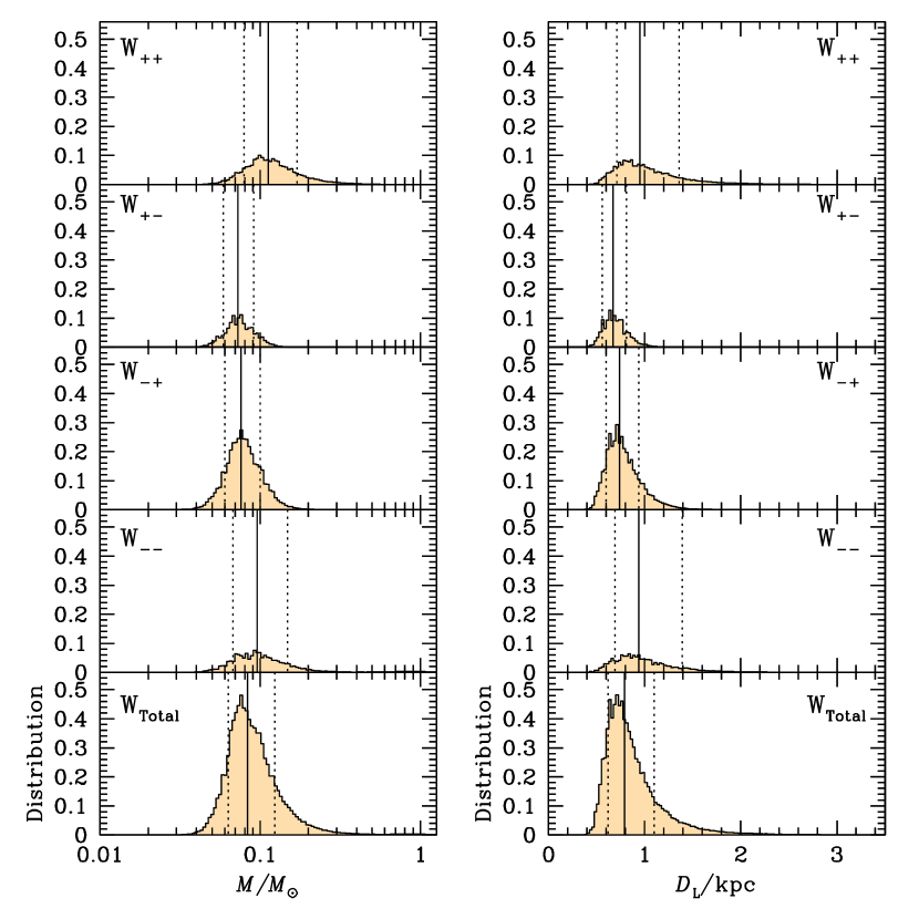
Figure 6: Histogram of wide solutions. The plot is similar to Figure 5. However, the overall scale is lower by a factor of roughly five because these solutions are less favored by both $\chi^{2}$ and the Galactic model.

The upper four sets of panels in Figures 5 and 6 show histograms for the lens mass and distance for each of the four close solutions and each of the four wide solutions, respectively. In each case, the relative area under the curve is the result of the weightings described by Equations (11)–(13). The relative weights can be evaluated from the last two columns of Table 4. In the bottom two panels of each figure, we show the combined histograms.

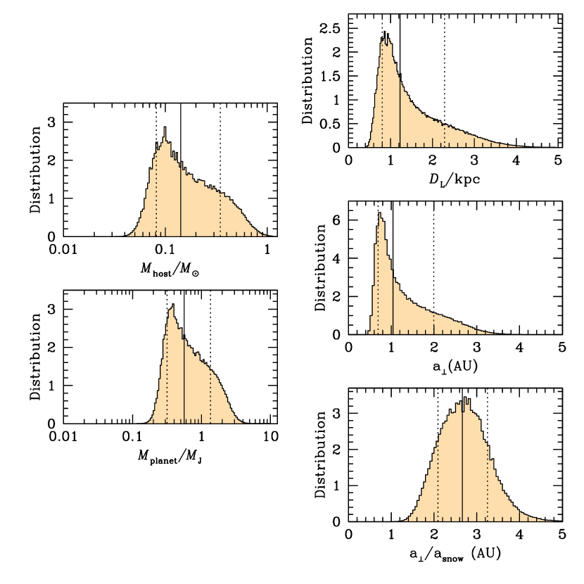
Figure 7: Posterior distributions of five physical quantities: host mass, planet mass, system distance, plant-host projected separation, and projected separation normalized to the snow line. Despite the parallax measurement, the allowed mass range in quite broad. Unless the lens proves to be substellar (for which there is only a small probability), its mass and distance will be decisively resolved at first light of next-generation (30m) telescopes.

The first point to note is that, overall, the close solutions are significantly favored. This is mainly due to the fact that the $C_{++}$ solution has the highest combined weight, which in turn reflects that it is compatible with disk lenses at relatively large distances (1–3 kpc), where the observation cone contains substantially more stars. The relatively broad range of lens distances of the dominant $C_{++}$ solution (together with the well constrained $\theta_{\rm E}=\sqrt{\kappa M\pi_{\rm rel}}$), likewise implies a relative broad distribution of lens masses. We conclude that the lens is very likely to be a low-mass star, within a factor of two of $M=0.1.5\,M_{\odot}$, at a distance of 0.8–2.3 kpc. See Figure 7. Because both the “wide” and “close” solutions have normalized separation $s$ quite close to unity, they do not substantially differ in their implications for the host-planet projected separation $a_{\perp}\equiv s\theta_{\rm E}D_{L}$: the uncertainty in this quantity is dominated by the uncertain source distance. This uncertainty mainly factors out if we normalize this projected separation to the snow line, for which we adopt $a_{\rm snow}=2.7{\rm au}(M/M_{\odot})$,

$${a_{\perp}\over a_{\rm snow}}={\kappa M_{\odot}s/2.7\over\theta_{\rm E}+\pi_{s}/\pi_{\rm E}}\simeq{(3\,{\rm mas})s\over\theta_{\rm E}+\pi_{s}/\pi_{\rm E}}$$ (14)

Thus, for very nearby lenses, i.e., $\pi_{\rm E}\gg\pi_{s}$, $a_{\perp}/a_{\rm snow}\rightarrow 3.4$, whereas for relatively distant lenses (within the framework of the Bayesian posteriors), $D_{L}\sim 3\,{\rm kpc}$, $a_{\perp}/a_{\rm snow}\rightarrow 2.0$. That is, the lens lies projected well outside the snow line over almost all of the posterior probability distribution.

5 Discussion

Despite a reasonably strong microlens parallax signal, the mass and distance of KMT-2018-BLG-1990 remain uncertain at the factor two level. Nevertheless, a Bayesian analysis combined with the parallax measurement shows that the lens is very likely to be a low mass M dwarf orbited by a gas giant planet in the Saturn-to-Jupiter mass range.

The relatively high lens-source relative proper motion $\mu_{\rm rel}\simeq 7\,{\rm mas}\,{\rm yr}^{-1}$ implies that by 2028 (i.e., the roughly expected adaptive-optics (AO) first light on next-generation 30m telescopes), the lens and source will be separated by about 70 mas, which is easily enough to separately resolve them. At that time the remaining uncertainty in the lens mass and distance can be resolved. According to the Bayesian analysis presented in Section 4.3, there is a small chance that the lens is below the hydrogen-burning limit, in which case it would most likely not be detected in such AO follow-up observation. Even in this case, however, it would be known to be a substellar object.

This is the second KMT-only Jovian planet that has been detected in the $44\,\rm deg^{2}$ of low-cadence $\Gamma\sim 0.4\,{\rm hr}^{-1}$ KMTNet observations. This confirms the naive expectation, which we outlined in Section 1, that KMTNet’s 3-site survey at this cadence should be sensitive to such planets. Improving statistics on this population is crucial to our understanding of planet formation and early orbital evolution of planetary systems. Guided in part by the observed planet-mass distribution in the Solar System and in part by theoretical consideration, it has long been predicted that the outer parts of extra-solar planetary systems should show a “gap” between Neptune-mass and Jovian-mass planets. Yet, the analysis of microlensing surveys (the only available means at present to probe cold planets that may lie in this gap) do not confirm these expectations. By obtaining a substantial sample of planets in this range, one can lay the basis for measuring their masses in subsequent AO followup observations, thus permitting a much stronger test of the “gap” hypothesis.

(15)

Table 1: Standard models

	Close	Wide
$\chi^{2}/\rm{dof}$	786.061/749	788.832/749
$t_{0}$ $(\rm{HJD}^{\prime})$	8230.495 $\pm$ 0.019	8230.370 $\pm$ 0.021
$u_{0}$	0.044 $\pm$ 0.001	0.039 $\pm$ 0.001
$t_{\rm E}$ $(\rm{days})$	43.929 $\pm$ 0.754	45.299 $\pm$ 0.984
$s$	0.968 $\pm$ 0.001	1.146 $\pm$ 0.004
$q$ $(10^{-3})$	3.723 $\pm$ 0.167	6.229 $\pm$ 0.315
$\alpha$ $(\rm{rad})$	2.559 $\pm$ 0.007	2.482 $\pm$ 0.007
$\rho$ $(10^{-3})$	1.280 $\pm$ 0.144	1.260 $\pm$ 0.155
$f_{S}$	0.356 $\pm$ 0.008	0.344 $\pm$ 0.010
$f_{B}$	0.147 $\pm$ 0.007	0.158 $\pm$ 0.008
$t_{*}$ $(\rm{days})$	0.056 $\pm$ 0.006	0.057 $\pm$ 0.007

Note. — Zerpoint for fluxes is 18, e.g., $I_{S}=18-2.5\log(f_{S})$.

Table 2: Parallax+orbital motion models for the close-separation

	$u_{0}>0$			$u_{0}<0$
Parameters	$\pi_{\rm{E},\it{N}}>0$	$\pi_{\rm{E},\it{N}}<0$		$\pi_{\rm{E},\it{N}}>0$	$\pi_{\rm{E},\it{N}}<0$
$\chi^{2}/\rm{dof}$	743.899/745	742.074/745		742.013/745	743.720/745
$t_{0}$ $(\rm{HJD}^{\prime})$	8230.449 $\pm$ 0.024	8230.466 $\pm$ 0.024		8230.465 $\pm$ 0.024	8230.448 $\pm$ 0.023
$u_{0}$	0.040 $\pm$ 0.002	0.043 $\pm$ 0.002		-0.043 $\pm$ 0.002	-0.040 $\pm$ 0.002
$t_{\rm E}$ $(\rm{days})$	46.484 $\pm$ 1.945	45.372 $\pm$ 1.760		45.908 $\pm$ 2.228	46.223 $\pm$ 2.260
$s$	0.963 $\pm$ 0.003	0.960 $\pm$ 0.007		0.963 $\pm$ 0.007	0.963 $\pm$ 0.005
$q$ $(10^{-3})$	3.748 $\pm$ 0.253	3.648 $\pm$ 0.370		3.529 $\pm$ 0.359	3.774 $\pm$ 0.303
$\alpha$ $(\rm{rad})$	2.584 $\pm$ 0.018	2.488 $\pm$ 0.017		3.794 $\pm$ 0.021	3.699 $\pm$ 0.020
$\rho$ $(10^{-3})$	1.187 $\pm$ 0.162	1.423 $\pm$ 0.150		1.388 $\pm$ 0.157	1.228 $\pm$ 0.159
$\pi_{\rm{E},\it{N}}$	1.147 $\pm$ 0.349	-1.428 $\pm$ 0.273		1.386 $\pm$ 0.262	-1.122 $\pm$ 0.355
$\pi_{\rm{E},\it{E}}$	0.140 $\pm$ 0.031	0.211 $\pm$ 0.046		0.198 $\pm$ 0.049	0.146 $\pm$ 0.034
$ds/dt$ $(\rm{yr}^{-1})$	0.503 $\pm$ 0.232	-0.695 $\pm$ 0.574		-0.359 $\pm$ 0.539	0.509 $\pm$ 0.548
$d\alpha/dt$ $(\rm{yr}^{-1})$	-0.302 $\pm$ 1.197	-4.136 $\pm$ 1.764		4.139 $\pm$ 2.294	0.163 $\pm$ 1.244
$f_{S}$	0.325 $\pm$ 0.016	0.353 $\pm$ 0.015		0.347 $\pm$ 0.018	0.328 $\pm$ 0.017
$f_{B}$	0.176 $\pm$ 0.016	0.151 $\pm$ 0.014		0.154 $\pm$ 0.017	0.175 $\pm$ 0.017
$t_{*}$ $(\rm{days})$	0.055 $\pm$ 0.007	0.065 $\pm$ 0.007		0.064 $\pm$ 0.007	0.057 $\pm$ 0.007
$\beta$	0.018 $\pm$ 0.111	0.653 $\pm$ 0.217		0.666 $\pm$ 0.201	0.016 $\pm$ 0.154

Note. — The parameter $\beta$ is restricted to $\beta<0.8$.

Table 3: Parallax+orbital motion models for the wide-separation

	$u_{0}>0$			$u_{0}<0$
Parameters	$\pi_{\rm{E},\it{N}}>0$	$\pi_{\rm{E},\it{N}}<0$		$\pi_{\rm{E},\it{N}}>0$	$\pi_{\rm{E},\it{N}}<0$
$\chi^{2}/\rm{dof}$	746.620/745	743.078/745		742.497/745	745.785/745
$t_{0}$ $(\rm{HJD}^{\prime})$	8230.343 $\pm$ 0.030	8230.405 $\pm$ 0.025		8230.400 $\pm$ 0.027	8230.327 $\pm$ 0.024
$u_{0}$	0.039 $\pm$ 0.002	0.035 $\pm$ 0.002		-0.037 $\pm$ 0.002	-0.039 $\pm$ 0.002
$t_{\rm E}$ $(\rm{days})$	45.646 $\pm$ 1.833	53.380 $\pm$ 2.721		51.389 $\pm$ 3.152	46.228 $\pm$ 1.870
$s$	1.115 $\pm$ 0.012	1.099 $\pm$ 0.009		1.095 $\pm$ 0.010	1.118 $\pm$ 0.009
$q$ $(10^{-3})$	5.591 $\pm$ 0.432	4.171 $\pm$ 0.418		4.185 $\pm$ 0.485	5.695 $\pm$ 0.335
$\alpha$ $(\rm{rad})$	2.530 $\pm$ 0.015	2.504 $\pm$ 0.011		3.781 $\pm$ 0.016	3.750 $\pm$ 0.015
$\rho$ $(10^{-3})$	1.223 $\pm$ 0.158	1.175 $\pm$ 0.140		1.246 $\pm$ 0.155	1.336 $\pm$ 0.160
$\pi_{\rm{E},\it{N}}$	1.400 $\pm$ 0.287	-1.649 $\pm$ 0.208		1.637 $\pm$ 0.252	-1.521 $\pm$ 0.370
$\pi_{\rm{E},\it{E}}$	0.075 $\pm$ 0.047	-0.003 $\pm$ 0.038		-0.002 $\pm$ 0.043	0.056 $\pm$ 0.034
$ds/dt$ $(\rm{yr}^{-1})$	-3.580 $\pm$ 1.249	-4.464 $\pm$ 0.727		-4.762 $\pm$ 0.098	-3.429 $\pm$ 0.855
$d\alpha/dt$ $(\rm{yr}^{-1})$	-0.367 $\pm$ 1.397	0.288 $\pm$ 0.665		-0.156 $\pm$ 1.269	-0.033 $\pm$ 0.348
$f_{S}$	0.334 $\pm$ 0.016	0.294 $\pm$ 0.017		0.307 $\pm$ 0.020	0.329 $\pm$ 0.017
$f_{B}$	0.169 $\pm$ 0.016	0.209 $\pm$ 0.017		0.195 $\pm$ 0.020	0.175 $\pm$ 0.017
$t_{*}$ $(\rm{days})$	0.056 $\pm$ 0.007	0.063 $\pm$ 0.007		0.064 $\pm$ 0.007	0.062 $\pm$ 0.007
$\beta$	0.567 $\pm$ 0.187	0.625 $\pm$ 0.144		0.750 $\pm$ 0.187	0.477 $\pm$ 0.133

Note. — The parameter $\beta$ is restricted to $\beta<0.8$.

Table 4: Physical properties

	Physical Properties					Relative Weights
Models	$M_{\rm host}$ $[M_{\sun}]$	$M_{\rm planet}$ $[M_{J}]$	$D_{\rm L}$ [kpc]	$a_{\bot}$ [au]		Gal.Mod.	$\chi^{2}$
$C_{++}$	$0.235_{-0.104}^{+0.187}$	$0.923_{-0.409}^{+0.734}$	$1.735_{-0.651}^{+0.889}$	$1.521_{-0.555}^{+0.753}$		1.000	0.390
$C_{+-}$	$0.084_{-0.019}^{+0.026}$	$0.323_{-0.071}^{+0.100}$	$0.873_{-0.165}^{+0.249}$	$0.689_{-0.103}^{+0.171}$		0.067	0.970
$C_{-+}$	$0.094_{-0.024}^{+0.036}$	$0.348_{-0.087}^{+0.132}$	$0.967_{-0.212}^{+0.308}$	$0.763_{-0.145}^{+0.219}$		0.171	1.000
$C_{--}$	$0.153_{-0.054}^{+0.311}$	$0.605_{-0.215}^{+1.229}$	$1.277_{-0.422}^{+1.629}$	$1.083_{-0.315}^{+1.353}$		0.189	0.425
$C_{\rm Total}$	$0.153_{-0.068}^{+0.206}$	$0.594_{-0.272}^{+0.814}$	$1.296_{-0.452}^{+1.061}$	$1.095_{-0.391}^{+0.953}$
$W_{++}$	$0.111_{-0.031}^{+0.057}$	$0.649_{-0.181}^{+0.330}$	$0.950_{-0.238}^{+0.411}$	$0.947_{-0.203}^{+0.377}$		0.159	0.100
$W_{+-}$	$0.073_{-0.014}^{+0.018}$	$0.318_{-0.058}^{+0.077}$	$0.674_{-0.115}^{+0.139}$	$0.657_{-0.075}^{+0.097}$		0.017	0.587
$W_{-+}$	$0.076_{-0.016}^{+0.023}$	$0.333_{-0.068}^{+0.101}$	$0.742_{-0.138}^{+0.201}$	$0.699_{-0.107}^{+0.145}$		0.039	0.785
$W_{--}$	$0.095_{-0.027}^{+0.053}$	$0.565_{-0.161}^{+0.316}$	$0.937_{-0.243}^{+0.457}$	$0.883_{-0.207}^{+0.379}$		0.078	0.152
$W_{\rm Total}$	$0.083_{-0.020}^{+0.039}$	$0.398_{-0.112}^{+0.291}$	$0.789_{-0.169}^{+0.316}$	$0.751_{-0.137}^{+0.283}$
${\rm Total}$	$0.141_{-0.061}^{+0.202}$	$0.565_{-0.249}^{+0.789}$	$1.229_{-0.427}^{+1.063}$	$1.039_{-0.351}^{+0.951}$

Figure 3: Scatter plots from the MCMC of the four solutions (close,wide)$\times(u_{0}<0,u_{0}>0)$ of KMT-2018-BLG-1990. Each shows two distinct minima, which correspond to the jerk-parallax degeneracy. Models with $\Delta\chi^{2}<(1^{2},2^{2},\ldots 10^{2})$ are shown in (red, gold, green, cyan, blue, magenta, black, dark gray, medium gray, light gray), respectively. Note that the abscissa and ordinate axis scales are incommensurate.

References

- Alard & Lupton (1998) Alard, C. & Lupton, R.H.,1998, ApJ, 503, 325
- Albrow et al. (2009) Albrow, M. D., Horne, K., Bramich, D. M., et al. 2009, MNRAS, 397, 2099
- Albrow (2017) Albrow, M. D., MichaelDAlbrow/pyDIA: Initial Release on Github, doi:10.5281/zenodo.268049
- Bensby et al. (2013) Bensby, T. Yee, J.C., Feltzing, S. et al. 2013, A&A, 549A, 147
- Bessell & Brett (1988) Bessell, M.S., & Brett, J.M. 1988, PASP, 100, 1134
- Gould (1992) Gould, A. 1992, ApJ, 392, 442
- Gould (2000) Gould, A. 2000, ApJ, 542, 785
- Gould (2004) Gould, A. 2004, ApJ, 606, 319
- Gould & Loeb (1992) Gould, A. & Loeb, A. 1992, ApJ, 396, 104
- Gould et al. (2013) Gould, A., Carey, S., & Yee, J. 2013, 2013spitz.prop.10036
- Gould et al. (2014) Gould, A., Carey, S., & Yee, J. 2014, 2014spitz.prop.11006
- Gould et al. (2015a) Gould, A., Yee, J., & Carey, S., 2015a, 2015spitz.prop.12013
- Gould et al. (2015b) Gould, A., Yee, J., & Carey, S. 2015b, 2016spitz.prop.12015
- Gould et al. (2016) Gould, A., Carey, S., & Yee, J. 2016, 2016spitz.prop.13005
- Gould et al. (2018) Gould, A., Yee, J., Carey, S., & Shvartzvald, Y. 2018, 2018spitz.prop.14012
- Griest & Safizadeh (1998) Griest, K. & Safizadeh, N. 1998, ApJ, 500, 37
- Henderson et al. (2014) Henderson, C.B., Gaudi, B.S., Han, c., et al. 2014, ApJ, 794, 52
- Jung et al. (2018) Jung, Y. K., Udalski, A., Gould, A., 2018 AJ, 155, 219
- Kervella et al. (2004) Kervella, P., Thévenin, F., Di Folco, E., & Ségransan, D. 2004, A&A, 426, 297
- Kim et al. (2016) Kim, S.-L., Lee, C.-U., Park, B.-G., et al. 2016, JKAS, 49, 37
- Kim et al. (2018a) Kim, D.-J., Kim, H.-W., Hwang, K.-H., et al., 2018a, AJ, 155, 76
- Kim et al. (2018c) Kim, H.-W., Hwang, K.-H., Kim, D.-J., et al., 2018c, AAS submitted, arXiv:1804.03352
- Kim et al. (2018d) Kim, H.-W., Hwang, K.-H., Shvartzvald, Y. et al., 2018d, AAS submitted, arXiv:1806.07545
- Mao & Paczyński (1991) Mao, S. & Paczyński, B. 1991, ApJ, 374, 37
- Nataf et al. (2013) Nataf, D.M., Gould, A., Fouqué, P. et al. 2013, ApJ, 769, 88
- Paczyński (1986) Paczyński, B. 1986, ApJ, 304, 1
- Park et al. (2004) Park, B.-G., DePoy, D.L.., Gaudi, B.S., et al. 2004, ApJ, 609, 166
- Skowron et al. (2011) Skowron, J., Udalski, A., Gould, A et al. 2011, ApJ, 738, 87
- Udalski et al. (2005) Udalski, A., Jaroszyński, M., Paczyński, B, et al. 2005, ApJ, 628, L109.
- Woźniak (2000) Woźniak, P. R. 2000, Acta Astron., 50, 421
- Zang et al. (2018) Zang, W., Hwang, K.-H., Kim, H.-W., et al. 2018, AJ, 156, 236