Merton’s portfolio problem under Volterra Heston model

Abstract

This paper investigates Merton’s portfolio problem in a rough stochastic environment described by Volterra Heston model. The model has a non-Markovian and non-semimartingale structure. By considering an auxiliary random process, we solve the portfolio optimization problem with the martingale optimality principle. Optimal strategies for power and exponential utilities are derived in semi-closed form solutions depending on the respective Riccati-Volterra equations. We numerically examine the relationship between investment demand and volatility roughness.
Keywords: Optimal portfolio, rough volatility, Volterra Heston model, Riccati-Volterra equations, utility maximization
Mathematics Subject Classification: 93E20, 60G22, 49N90, 60H10.

1 Introduction

Empirical studies suggest that implied and realized volatilities of major financial indices tend to have rougher sample paths than the ones modeled by the standard Brownian motion (Gatheral et al., 2018). This discovery stimulates a rapidly growing development in rough volatility models recently. This new generation of models are constructed with stochastic processes such as fractional Brownian motion (fBm), fractional Ornstein-Uhlenbeck (fOU) process, and rough Bergomi (rBergomi) model. Recent empirical studies suggest that roughness is also associated with market fear (Caporale et al., 2018) and risks in pension fund portfolios (Cadoni et al., 2017).

The popularity of the Heston model in the financial market leads to the introduction of the fractional Heston model (Guennoun et al., 2018) and the rough Heston model (El Euch and Rosenbaum, 2019). Both are rough versions of the celebrated Heston stochastic volatility model. Compared with classic Heston model, rough Heston model (El Euch and Rosenbaum, 2019) builds on market microstructure and better captures the explosion of at-the-money (ATM) skew, as illustrated in Figures (1)-(1). Other motivations and properties of rough volatility models can be found in Gatheral et al. (2018); El Euch and Rosenbaum (2019). Recent remarkable advances include the derivation of the characteristic function of the rough Heston model (El Euch and Rosenbaum, 2019) and the affine Volterra processes (Abi Jaber et al., 2019). The Volterra Heston model serves as an important specific example in Abi Jaber et al. (2019). In addition, the rough Heston model becomes a special case of Volterra Heston model under the fractional kernel. The structure of characteristic functions in El Euch and Rosenbaum (2019) can be extended to affine Volterra processes using Riccati-Volterra equations as shown in Abi Jaber et al. (2019). Therefore, this paper focuses on the financial market with the Volterra Heston model.

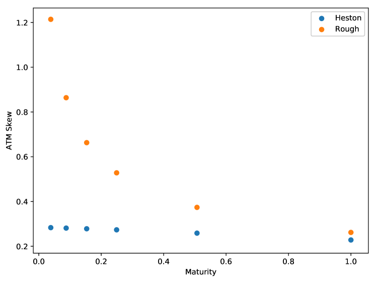
(a) ATM skew of Heston and rough Heston model

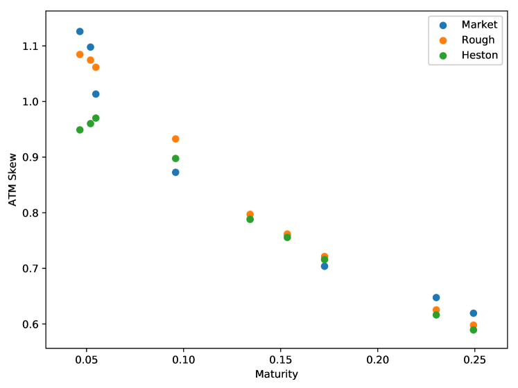
(b) Calibration

Figure 1: ATM skew. Left subplot gives a theoretical comparison. For rough Heston model, parameters are $H=0.12$, $\phi=0.3156$, $\kappa=0.1$, $\rho=-0.681$, $\sigma=1.044$, $V_{0}=0.0392$. For classic Heston model, let $H=0.5$ and others unchanged. Rough Heston model captures the explosion of ATM skew easily. The right subplot illustrates calibration based on S&P 500 implied volatility surface on 03/29/2019. For rough Heston model, parameters are $H=0.118$, $\phi=0.170$, $\kappa=0.173$, $\rho=-0.615$, $\sigma=0.340$, $V_{0}=0.0182$. For classic Heston model, $\phi=0.037$, $\kappa=5.609$, $\rho=-0.614$, $\sigma=1.188$, $V_{0}=0.015$. Classic Heston model obtains larger $\kappa$ and $\sigma$, but it still fails to model the explosion of ATM skew, observed from the market data when the maturity approaches zero. We refer readers to (6) for notations.

How does the roughness of the market volatility affect investment demands? We address this by investigating the optimal investment demand with the Merton problem as it is probably the most classic financial economic approach to do so (Merton, 1969; Kraft, 2005; Hu et al., 2005; Jang and Park, 2014). The literature tends to focus more on the option pricing problems and portfolio optimization under rough volatility models is still at an early stage. However, some recent works do exist, see Fouque and Hu (2019, 2018); Bäuerle and Desmettre (2018); Glasserman and He (2019); Han and Wong (2019a, b) and references therein. The studies in Fouque and Hu (2019, 2018) consider the expected power utility portfolio maximization with slow or fast varying stochastic factors driven by the fOU processes whereas the fractional Heston model (Guennoun et al., 2018) is used in Bäuerle and Desmettre (2018) with the same objective function. Inspired by some market insights, it is suggested in Glasserman and He (2019) to use roughness as a trading signal. To the best of our knowledge, portfolio selection with Volterra Heston model is firstly studied in Han and Wong (2019a) in the context of mean-variance objective.

In this paper, we investigate Merton’s portfolio problem with an unbounded risk premium. To overcome the difficulty from the non-Markovian and non-semimartingale characteristic in Volterra Heston model, we apply the martingale optimality principle (Hu et al., 2005; Pham, 2009; Jeanblanc et al., 2012) and construct the Ansatz, which is inspired by the martingale distortion transformation (Zariphopoulou, 2001; Fouque and Hu, 2019) and the exponential-affine representations (Abi Jaber et al., 2019). The key finding is the auxiliary processes $M_{t}$ in (15) and (27) with properties presented in Theorem 3.2 and 3.5 below. We offer explicit solutions to the optimal portfolio policies that depend on Riccati-Volterra equations, which can be solved by well-known numerical methods. Our result differs from previous literature as follows:

• Hu et al. (2005); Fouque and Hu (2019, 2018) assume an essentially bounded risk premium. This assumption does not hold for the Volterra Heston model so that their results cannot be applied here.

• Compared with Bäuerle and Desmettre (2018), we consider different models and provide explicit solutions for a non-zero correlation between stock and volatility, reflecting the well-known market leverage effect.

• Although the power utility maximization with the classic Heston model has been studied in Kraft (2005), the non-Markovian and non-semimartingale characteristic in Volterra Heston model prevents the use of the Hamilton-Jacobi-Bellman (HJB) framework for the classic model in Kraft (2005).

• The $M_{t}$ in (15) is unbounded, making the proof of Theorem 3.2 and 3.3 different from both Fouque and Hu (2019) and Han and Wong (2019a).

• We also consider the exponential utility. The corresponding wealth process is not necessarily bounded below. It complicates the proof in Theorem 3.6. Moreover, we provide an interesting comparison between power utility and exponential utility, from the perspective of rough volatility.

• Han and Wong (2019a) apply completion of squares technique which is tailor-made for mean-variance portfolio (MVP) problem, while this paper adopts martingale optimality principle. Mean-variance portfolio selection and expected utility theory are usually considered separately, due to the completely different objectives and solution methods. In addition, dynamic MVP may have to additionally address the issue of time inconsistency (Chen and Wong, 2019; Han and Wong, 2019b).

By deriving the analytical optimal investment demand, we are able to discuss the effect of volatility roughness on investment decisions. In rough Heston market, our sensitivity analysis suggests that investors with a power utility demand less on the stock market if the stock volatility is rougher whereas investors with an exponential utility demand more although both types of investors are risk averse. We further expand our analysis to parameters calibrated to simulated option data. The behaviors remain different for these two types of investors, documenting a significant difference in economic results for these two utility functions.

The rest of this paper is organized as follows. We present the problem formulation in Section 2 and solve the problem by the martingale optimality principle in Section 3. Section 4 offers numerical illustration for the investment demand under the rough Heston model. Section 5 concludes. All technical proofs are put into Appendix A.

2 Problem formulation

Let $(\Omega,{\mathcal{F}},\mathbb{P})$ be a complete probability space, with a filtration $\mathbb{F}=\{{\mathcal{F}}_{t}\}_{0\leq t\leq T}$ satisfying the usual conditions, supporting a two-dimensional Brownian motion $W=(W_{1},W_{2})$. The filtration $\mathbb{F}$ is not necessarily the augmented filtration generated by $W$.

Denote a kernel $K(\cdot)\in L^{2}_{loc}(\mathbb{R}_{+},\mathbb{R})$ where $\mathbb{R}_{+}=\{t\in\mathbb{R}|t\geq 0\}$. Suppose the standing Assumption 2.1 holds throughout the paper, in line with Abi Jaber et al. (2019); Keller-Ressel et al. (2018); Han and Wong (2019a, b). Recall that a function $f$ is completely monotone on $(0,\infty)$, if it is infinitely differentiable on $(0,\infty)$ and $(-1)^{k}f^{(k)}(t)\geq 0$ for all $t>0$, $k=0,1,...$. Assumption 2.1 is satisfied by positive constant kernels, fractional kernels and exponential kernels, with proper parameters, see Abi Jaber et al. (2019).

Assumption 2.1.

The kernel $K$ is strictly positive and completely monotone on $(0,\infty)$. There is $\delta\in(0,2]$ such that $\int_{0}^{h}K(t)^{2}dt=O\left(h^{\delta}\right)$ and $\int_{0}^{T}(K(t+h)-K(t))^{2}dt=O(h^{\delta})$ for every $T<\infty$.

The convolution $K*L$ for a measurable kernel $K$ on $\mathbb{R}_{+}$ and a measure $L$ on $\mathbb{R}_{+}$ of locally bounded variation is defined by

$$(K*L)(t)=\int^{t}_{0}K(t-s)L(ds)$$ (1)

for $t>0$ under proper conditions. The integral is extended to $t=0$ by right-continuity if possible. If $F$ is a function on $\mathbb{R}_{+}$, let

$$(K*F)(t)=\int_{0}^{t}K(t-s)F(s)ds.$$ (2)

For a $1$-dimensional continuous local martingale $W$, the convolution between $K$ and $W$ is defined as

$$(K*dW)_{t}=\int_{0}^{t}K(t-s)dW_{s}.$$ (3)

A measure $L$ on $\mathbb{R}_{+}$ is called resolvent of the first kind to $K$, if

$$K*L=L*K\equiv\rm{id}.$$ (4)

The existence of a resolvent of the first kind is shown in Gripenberg et al. (1990, Theorem 5.5.4) under the complete monotonicity assumption, imposed in Assumption 2.1. Alternative conditions for the existence are given in Gripenberg et al. (1990, Theorem 5.5.5).

Kernel $R$ is called the resolvent, or resolvent of the second kind, to $K$ if

$$K*R=R*K=K-R.$$ (5)

The resolvent always exists and is unique by Gripenberg et al. (1990, Theorem 2.3.1). Further properties of these definitions can be found in Gripenberg et al. (1990); Abi Jaber et al. (2019). Examples of kernels are available at Abi Jaber et al. (2019, Table 1).

The variance process of the Volterra Heston model is defined as

$$V_{t}=V_{0}+\kappa\int_{0}^{t}K(t-s)\left(\phi-V_{s}\right)ds+\int_{0}^{t}K(t-s)\sigma\sqrt{V_{s}}dB_{s},$$ (6)

where $dB_{s}=\rho dW_{1s}+\sqrt{1-\rho^{2}}dW_{2s}$ and $V_{0},\kappa,\phi,\sigma$ are positive constants. The correlation $\rho$ between stock price and variance is also assumed constant. The process in (6) is non-Markovian and non-semimartingale in general. Rough Heston model in El Euch and Rosenbaum (2019, 2018) is a special case of (6) with $K(t)=\frac{t^{H-1/2}}{\Gamma(H+1/2)}$, $H\in(0,1/2]$. An alternative definition for Heston model with rough paths in Guennoun et al. (2018) is known as fractional Heston model.

Suppose there is a risk-free asset with deterministic bounded risk-free rate $r_{t}>0$. Following Abi Jaber et al. (2019); Kraft (2005), we assume the risky asset (stock or index) price $S_{t}$ follows

$$dS_{t}=S_{t}(r_{t}+\theta V_{t})dt+S_{t}\sqrt{V_{t}}dW_{1t},\quad S_{0}>0,$$ (7)

with constant $\theta\neq 0$. Then the market price of risk (risk premium) is given by $\theta\sqrt{V_{t}}$.

We need the following existence and uniqueness result.

Theorem 2.2.

(Theorem 7.1 in Abi Jaber et al. (2019)) Under Assumption 2.1, the stochastic Volterra equation (6)-(7) has a unique in law $\mathbb{R}_{+}\times\mathbb{R}_{+}$-valued continuous weak solution for any initial condition $(S_{0},V_{0})\in\mathbb{R}_{+}\times\mathbb{R}_{+}$.

For strong uniqueness, we mention Abi Jaber and El Euch (2019, Proposition B.3) as a related result with kernel $K\in C^{1}([0,T],\mathbb{R})$ and Mytnik and Salisbury (2015, Proposition 8.1) for certain Volterra integral equations with smooth kernels. The strong uniqueness of (6)-(7) is left open for singular kernels. For weak solutions, Brownian motion is also a part of the solution. However, expected utility only depends on the expectation of the wealth process. In the sequel, we fix a version of the solution $(S,V,W_{1},W_{2})$ to (6)-(7) as other solutions have the same law.

Merton problem aims at

$$\sup_{\alpha(\cdot)\in{\mathcal{A}}}\mathbb{E}\left[U(X_{T})\right],$$ (8)

where $\alpha$ is an admissible investment strategy introduced later and $X$ is the corresponding wealth. $U(\cdot)$ is a utility function. Specifically, we consider power utility and exponential utility in this paper. The classic martingale optimality principle, see, e.g., Hu et al. (2005), Pham (2009, Section 6.6.1) or Jeanblanc et al. (2012), states that the Problem (8) can be solved by constructing a family of processes $\{J^{\alpha}_{t}\}_{t\in[0,T]}$, $\alpha\in{\mathcal{A}}$, satisfying conditions:

1. $J^{\alpha}_{T}=U(X_{T})$ for all $\alpha\in{\mathcal{A}}$;

2. $J^{\alpha}_{0}$ is a constant, independent of $\alpha\in{\mathcal{A}}$;

3. $J^{\alpha}_{t}$ is a supermartingale for all $\alpha\in{\mathcal{A}}$, and there exists $\alpha^{*}\in{\mathcal{A}}$ such that $J^{\alpha^{*}}$ is a martingale.

Indeed, if we can find $J^{\alpha}_{t}$, then for all $\alpha\in{\mathcal{A}}$,

$$\mathbb{E}[U(X_{T})]=\mathbb{E}[J^{\alpha}_{T}]\leq J^{\alpha}_{0}=J^{\alpha^{*}}_{0}=\mathbb{E}[J^{\alpha^{*}}_{T}]=\mathbb{E}[U(X^{*}_{T})],$$

where $X^{*}$ is the wealth process under $\alpha^{*}$.

3 Optimal strategy

3.1 Power utility

Let $\alpha_{t}\triangleq\sqrt{V_{t}}\pi_{t}$ be the investment strategy, where $\pi_{t}$ is the proportion of wealth invested in the stock. Then, the wealth process $X_{t}$ reads

$$dX_{t}=\big{(}r_{t}+\theta\sqrt{V_{t}}\alpha_{t}\big{)}X_{t}dt+\alpha_{t}X_{t}dW_{1t},\;X_{0}=x_{0}>0.$$ (9)

Definition 3.1.

An investment strategy $\alpha(\cdot)$ is said to be admissible if

1. $\alpha(\cdot)$ is $\mathbb{F}$-adapted and $\int^{T}_{0}\alpha^{2}_{s}ds<\infty$, $\mathbb{P}$-a.s.;

2. the wealth process (9) has a unique solution in the sense of Yong and Zhou (1999, Chapter 1, Definition 6.15), with $\mathbb{P}$-a.s. continuous paths;

3. $X_{t}\geq 0$, $\forall\;t\in[0,T]$, $\mathbb{P}$-a.s.;

4. $\mathbb{E}\Big{[}\frac{1}{\gamma}X^{\gamma}_{T}\Big{]}<\infty$, $0<\gamma<1$.

The set of all admissible investment strategies is denoted as ${\mathcal{A}}$.

We are interested in the power utility optimization:

$$\sup_{\alpha(\cdot)\in{\mathcal{A}}}\mathbb{E}\left[\frac{1}{\gamma}X^{\gamma}_{T}\right],\quad 0<\gamma<1.$$ (10)

To ease notation burden, we simply write $X$, instead of $X^{x_{0},\alpha}$, as the wealth process (9) under $\alpha\in{\mathcal{A}}$ with initial condition $X_{0}=x_{0}>0$.

To construct $J^{\alpha}_{t}$, we introduce a new probability measure $\tilde{\mathbb{P}}$ together with $\tilde{W}_{1t}\triangleq W_{1t}-\frac{\gamma\theta}{1-\gamma}\int^{t}_{0}\sqrt{V_{s}}ds$ as the new Brownian motion by Abi Jaber et al. (2019, Lemma 7.1). Under $\tilde{\mathbb{P}}$,

$$V_{t}=V_{0}+\int_{0}^{t}K(t-s)\left(\kappa\phi-\lambda V_{s}\right)ds+\int_{0}^{t}K(t-s)\sigma\sqrt{V_{s}}d\tilde{B}_{s},$$ (11)

with $\lambda=\kappa-\frac{\gamma}{1-\gamma}\rho\theta\sigma$ and $d\tilde{B}_{s}=\rho d\tilde{W}_{1s}+\sqrt{1-\rho^{2}}dW_{2s}$.

Denote $\tilde{\mathbb{E}}[\cdot]$ and $\tilde{\mathbb{E}}_{t}[\cdot]=\mathbb{\tilde{E}}[\cdot|{\mathcal{F}}_{t}]$ as the $\tilde{\mathbb{P}}$-expectation and conditional $\tilde{\mathbb{P}}$-expectation, respectively. The forward variance under $\tilde{\mathbb{P}}$ is the conditional $\tilde{\mathbb{P}}$-expected variance, that is, $\mathbb{\tilde{E}}_{t}[V_{s}]\triangleq\xi_{t}(s)$. It is shown in Keller-Ressel et al. (2018, Propsition 3.2) and Abi Jaber et al. (2019, Lemma 4.2) that

$$\xi_{t}(s)=\mathbb{\tilde{E}}\left[V_{s}|\mathcal{F}_{t}\right]=\xi_{0}(s)+\int_{0}^{t}\frac{1}{\lambda}R_{\lambda}(s-u)\sigma\sqrt{V_{u}}d\tilde{B}_{u},$$ (12)

where

$$\xi_{0}(s)=\left(1-\int_{0}^{s}R_{\lambda}(u)du\right)V_{0}+\frac{\kappa\phi}{\lambda}\int_{0}^{s}R_{\lambda}(u)du,$$ (13)

and $R_{\lambda}$ is the resolvent of $\lambda K$ such that

$$\lambda K*R_{\lambda}=R_{\lambda}*(\lambda K)=\lambda K-R_{\lambda}.$$ (14)

Consider the stochastic process,

$$M_{t}=\exp\Big{[}\int^{T}_{t}\big{(}\gamma r_{s}+\frac{\gamma\theta^{2}\xi_{t}(s)}{2(1-\gamma)}+\frac{c\sigma^{2}}{2}\psi^{2}(T-s)\xi_{t}(s)\big{)}ds\Big{]},$$ (15)

where $c=\frac{1-\gamma}{1-\gamma+\gamma\rho^{2}}$ and $\psi(\cdot)$ satisfies the Riccati-Volterra equation

$$\psi(t) =\int^{t}_{0}K(t-s)\big{[}\frac{\sigma^{2}}{2}\psi^{2}(s)-\lambda\psi(s)+\frac{\gamma\theta^{2}}{2c(1-\gamma)}\big{]}ds.$$ (16)

Existence and uniqueness of the solution to (16) are established in Han and Wong (2019a, Lemma A.2 and A.3) based on the results of Gatheral and Keller-Ressel (2019); El Euch and Rosenbaum (2018). Indeed, if $\lambda>0$ and $\lambda^{2}-\frac{\gamma\theta^{2}\sigma^{2}}{c(1-\gamma)}>0$, then (16) has a unique non-negative global solution. These assumptions are also in line with Kraft (2005, Proposition 5.2). Furthermore, there is a tighter result for (16) with the fractional kernel in El Euch and Rosenbaum (2018, Theorem 3.2).

By considering $M_{t}$, we overcome the non-Markovian and non-semimartingale difficulty in the variance process (6). Main properties of $M_{t}$ are summarized in Theorem 3.2. We highlight that the $M_{t}$ in (15) is unbounded so that it is very different from the one considered in Fouque and Hu (2019); Han and Wong (2019a).

Theorem 3.2.

Assume

$$\kappa^{2}-6\frac{\gamma^{2}}{(1-\gamma)^{2}}\theta^{2}\sigma^{2}>0,\quad\lambda>0,\quad\lambda^{2}-2p\frac{\gamma}{1-\gamma}\theta^{2}\sigma^{2}>0,$$ (17)

for some $p>1/(2c)$. Then $M$ has following properties:

1. $M_{t}\geq l>0$ for some positive constant $l$. And $\mathbb{E}\big{[}\sup_{t\in[0,T]}|M_{t}|^{p}\big{]}<\infty$;

2. Apply Itô’s lemma to $M$ on $t$, then

   $$dM_{t}= -\big{[}\gamma r_{t}+\frac{\gamma}{2(1-\gamma)}\theta^{2}V_{t}\big{]}M_{t}dt-\frac{\gamma}{2(1-\gamma)}\big{[}2\theta\sqrt{V_{t}}U_{1t}+\frac{U^{2}_{1t}}{M_{t}}\big{]}dt+U_{1t}dW_{1t}+U_{2t}dW_{2t},$$ (18)

   where

   $$U_{1t} =\rho c\sigma M_{t}\sqrt{V_{t}}\psi(T-t),$$ (19)

   $$U_{2t} =\sqrt{1-\rho^{2}}c\sigma M_{t}\sqrt{V_{t}}\psi(T-t).$$ (20)

3. $\mathbb{E}\Big{[}\big{(}\int^{T}_{0}U^{2}_{it}dt\big{)}^{p/4}\Big{]}<\infty$ for $i=1,2$.

Now we are ready to give the Ansatz for $J^{\alpha}_{t}$. Consider

$$J^{\alpha}_{t}=\frac{X^{\gamma}_{t}}{\gamma}M_{t}.$$ (21)

Then we have the following verification result.

Theorem 3.3.

Suppose the conditions (17) in Theorem 3.2 hold and $\kappa^{2}-2\eta\sigma^{2}>0$, where

$$\eta=\max\Big{\{}2q|\theta|\sup_{t\in[0,T]}|A_{t}|,(8q^{2}-2q)\sup_{t\in[0,T]}|A_{t}|^{2}\Big{\}},$$ (22)

for some $q>1$ and $A_{t}=\frac{1}{1-\gamma}\big{[}\theta+\rho c\sigma\psi(T-t)\big{]}$. Then $J^{\alpha}_{t}=\frac{X^{\gamma}_{t}}{\gamma}M_{t}$ satisfies the martingale optimality principle, and an optimal strategy is given by

$$\alpha^{*}_{t}=A_{t}\sqrt{V_{t}}.$$ (23)

Moreover,

$$\mathbb{E}\Big{[}\sup_{t\in[0,T]}|X^{*}_{t}|^{q}\Big{]}<\infty,$$ (24)

and $\alpha^{*}$ is admissible.

3.2 Exponential utility

In this subsection, we consider the exponential utility case. With a slightly different formulation, let $u_{t}$ be the investment strategy. The wealth process $X_{t}$ reads

$$dX_{t}=\big{(}r_{t}X_{t}+\theta\sqrt{V_{t}}u_{t}\big{)}dt+u_{t}dW_{1t},\;X_{0}=x_{0}>0.$$ (25)

The following admissibility assumption is consistent with Hu et al. (2005).

Definition 3.4.

Let $\gamma>0$, an investment strategy $u(\cdot)$ is said to be admissible if

1. $u(\cdot)$ is $\mathbb{F}$-adapted and $\mathbb{E}[\int^{T}_{0}u^{2}_{s}ds]<\infty$;

2. the wealth process (25) has a unique solution in the sense of Yong and Zhou (1999, Chapter 1, Definition 6.15), with $\mathbb{P}$-a.s. continuous paths;

3. $\{\exp\big{[}-\gamma e^{\int^{T}_{\tau}r_{v}dv}X_{\tau}\big{]}:\tau\text{ stopping time with values in }[0,T]\}$ is a uniformly integrable family.

The set of all admissible investment strategies is denoted as ${\mathcal{U}}$.

The investor now considers

$$\sup_{u(\cdot)\in{\mathcal{U}}}\mathbb{E}\left[-\frac{1}{\gamma}e^{-\gamma X_{T}}\right],\quad\gamma>0.$$ (26)

The solution method is similar to the power utility case. With slightly abuse of notations, we still use $\psi(\cdot)$, forward variance $\xi_{t}(s)$, $M$, etc. However, they are redefined and not mixed with counterparts in power utility case.

To construct $J^{u}_{t}$, we introduce a new probability measure $\tilde{\mathbb{P}}$ together with $\tilde{W}_{1t}\triangleq W_{1t}+\theta\int^{t}_{0}\sqrt{V_{s}}ds$ as the new Brownian motion and $\lambda=\kappa+\rho\sigma\theta$. Consider the stochastic process,

$$M_{t}=\exp\Big{[}\int^{T}_{t}\big{(}-\frac{\theta^{2}}{2}\xi_{t}(s)+\frac{\sigma^{2}(1-\rho^{2})}{2}\psi^{2}(T-s)\xi_{t}(s)\big{)}ds\Big{]},$$ (27)

where $\xi_{t}(s)$ is forward variance under $\tilde{\mathbb{P}}$ and $\psi(\cdot)$ satisfies

$$\psi(t) =\int^{t}_{0}K(t-s)\big{[}\frac{\sigma^{2}(1-\rho^{2})}{2}\psi^{2}(s)-\lambda\psi(s)-\frac{\theta^{2}}{2}\big{]}ds.$$ (28)

If $\lambda>0$, then (28) has a unique global solution.

Theorem 3.5.

Assume $\lambda>0$. Then $M$ in (27) has following properties:

1. $M_{t}$ is essentially bounded. $0<M_{t}\leq 1$, $\forall\;t\in[0,T]$, $\mathbb{P}$-a.s.;

2. Apply Itô’s lemma to $M$ on $t$, then

   $$dM_{t}=\frac{(\theta\sqrt{V_{t}}M_{t}+U_{1t})^{2}}{2M_{t}}dt+U_{1t}dW_{1t}+U_{2t}dW_{2t},$$ (29)

   where

   $$U_{1t}=\rho\sigma M_{t}\sqrt{V_{t}}\psi(T-t),\quad U_{2t}=\sqrt{1-\rho^{2}}\sigma M_{t}\sqrt{V_{t}}\psi(T-t).$$ (30)

3. $\mathbb{E}\Big{[}\big{(}\int^{T}_{0}U^{2}_{it}dt\big{)}^{p/2}\Big{]}<\infty$ for $p\geq 1$ and $i=1,2$.

Consider

$$J^{u}_{t}=-\frac{1}{\gamma}\exp\big{[}-\gamma e^{\int^{T}_{t}r_{s}ds}X_{t}\big{]}M_{t}.$$ (31)

Then we have the following verification result.

Theorem 3.6.

Suppose $\lambda>0$ and $\kappa^{2}-2\eta\sigma^{2}>0$ with

$$\eta=\sup_{t\in[0,T]}\Big{\{}2p^{2}\gamma^{2}e^{\int^{T}_{t}2r_{v}dv}A^{2}_{t}+2p\gamma e^{\int^{T}_{t}r_{v}dv}|\theta A_{t}|\Big{\}},\text{ for some }p>1,$$ (32)

where $A_{t}=\frac{1}{\gamma}e^{-\int^{T}_{t}r_{v}dv}\big{[}\theta+\rho\sigma\psi(T-t)\big{]}$. Then $J^{u}_{t}$ satisfies the martingale optimality principle. An optimal strategy is given by

$$u^{*}_{t}=A_{t}\sqrt{V_{t}},$$ (33)

and $u^{*}$ is admissible.

4 Investment under rough volatility

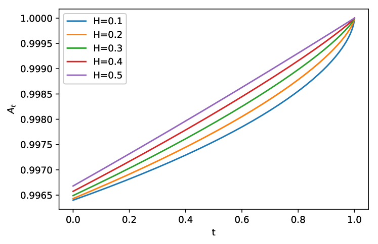
(a) $A_{t}$ under power utility

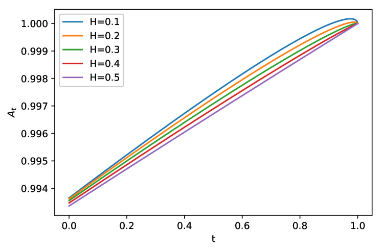
(b) $A_{t}$ under exponential utility

Figure 2: $A_{t}$ under different utility and $H$. We set risk-free rate $r=0.01$, risk aversion $\gamma=0.5$, volatility of volatility $\sigma=0.02$, mean-reversion speed $\kappa=0.1$, risk premium parameter $\theta=0.5$, correlation $\rho=-0.7$, and time horizon $T=1$.

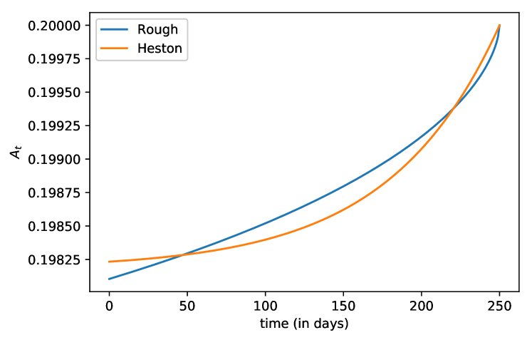
(a) $A_{t}$ under power utility

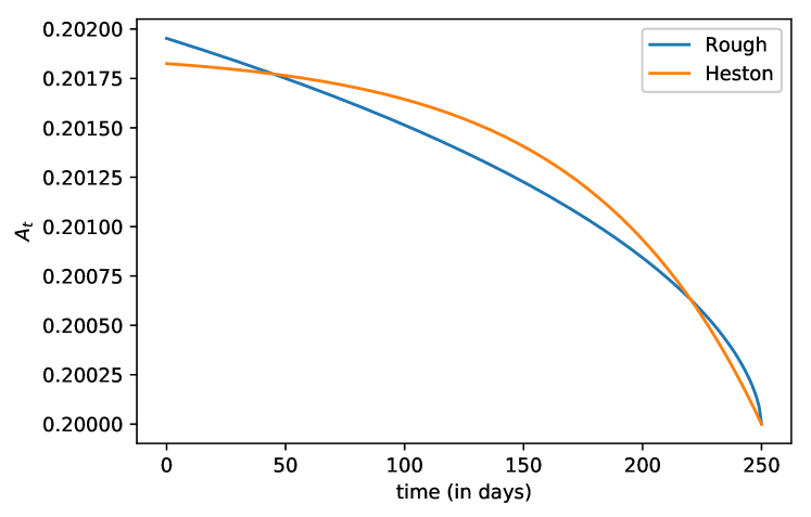
(b) $A_{t}$ under exponential utility

Figure 3: We set $250$ time steps for one year, corresponding to the $250$ trading days in a year. Risk-free rate $r=0$. Risk premium parameter $\theta=0.1$. Risk aversion $\gamma=0.5$. Other parameters are adopted from Abi Jaber (2019, Table 6) and Abi Jaber (2019, Table 4).

Both power utility and exponential utility have been widely adopted in literature. Different behaviors of these utility functions have been demonstrated before. Power utility has constant relative risk aversion, while exponential utility has constant absolute risk aversion. Optimal strategy under power utility is proportional to wealth. Therefore, it guarantees a non-negative wealth and avoids bankruptcy. In contrast, optimal strategy under exponential utility is not related to investor’s wealth. The proportion of wealth in the stock is lower for richer investors, since the dollar value in the stock is the same. Merton (1969) wrote that exponential utility is “behaviorially less plausible than constant relative risk aversion”. In our numerical study, we discover a new difference of these two utility functions from the perspective of roughness.

We consider the fractional kernel $K(t)=\frac{t^{H-1/2}}{\Gamma(H+1/2)}$, $H\in(0,1/2)$, corresponding to rough Heston model. The smaller the Hurst parameter $H$, the rougher the volatility of the stock. $H=\frac{1}{2}$ corresponds to the strategy in Kraft (2005) under the classic Heston model. We use the Adams method (El Euch and Rosenbaum, 2019; Han and Wong, 2019a) to solve the Riccati-Volterra equations (16) and (28) numerically. Figures (2)-(2) show the $A_{t}$ in $\alpha^{*}$ (23) and $u^{*}$ (33), under different values of $H$. Assumptions in Theorem 3.3 and 3.6 are satisfied by the parameter setting detailed in figure descriptions. Figure (2) exhibits that if the stock volatility is rougher, the investment demand (23) under power utility is smaller. It is partially due to the market leverage. In the equity market, the correlation $\rho$ is usually negative. $\psi(t)$ is positive for $t>0$. Moreover, the value of $\psi(t)$ becomes larger for a smaller $H$. Interestingly, exponential utility implies complete different opinion about roughness. It suggests investing more under smaller $H$.

We stress that Figures (2)-(2) are sensitivity analysis and demonstrate the marginal effect of roughness parameter. However, it is not plausible to only vary Hurst parameter $H$ while keeping other parameters unchanged. Therefore, we adopt a simulated implied volatility surface in Abi Jaber (2019). The investors calibrate two sets of parameters under classic Heston model and rough Heston model respectively, for the same implied volatility surface. The investor under the Heston model uses the calibrated parameters in Abi Jaber (2019, Table 6) to implement the optimal strategy. The investor under rough Heston model uses Abi Jaber (2019, Table 4) instead. Figures (3)-(3) illustrate the $A_{t}$ under power utility and exponential utility. Again, they have different opinions about investing less or more if rough Heston model is used. Moreover, Figures (2)-(2) and Figures (3)-(3) do not conflict with each other. The calibrated parameters in Abi Jaber (2019, Table 6) for classic Heston model have significantly larger mean-reversion and volatility-of-volatility parameters than the counterparts in rough Heston model.

There is no definite answer to the question that investors should invest more or less for different roughness, under expected utility theory. The type of risk aversions matters. Our discovery provides a new difference in utility preference by considering roughness. But the rationale behind is largely unexplained and needs more investigations. Moreover, expected utility theory also suffers some issues, see Aït-Sahalia and Hansen (2009, Chapter 5) and references therein.

5 Concluding remarks

In this paper, we solve Merton’s portfolio optimization under Volterra Heston model. Economically, this paper shows that different forms of risk aversion described by concave utility functions exhibit different sensitivity in investment demand with respect to the volatility roughness. Technically, we offer a novel solution approach for the Merton portfolio problem in a rough volatility economy based on the martingale optimality principle. The key is the recognition of a novel auxiliary stochastic process. A future direction is to incorporate model uncertainty.

Appendix A Proofs of main results

Proof of Theorem 3.2.

First of all, we point out that there exists a unique continuous solution to (16) over $[0,T]$ under Assumption (17). Then, we claim

$$M^{1/c}_{t}=\mathbb{\tilde{E}}_{t}\Big{[}\exp\Big{(}\int^{T}_{t}\big{(}\frac{\gamma}{c}r_{s}+\frac{\gamma}{2c(1-\gamma)}\theta^{2}V_{s}\big{)}ds\Big{)}\Big{]}.$$ (34)

Indeed, by Abi Jaber et al. (2019, Theorem 4.3),

$$\exp\Big{[}\int^{T}_{t}\big{(}\frac{\gamma\theta^{2}}{2c(1-\gamma)}\xi_{t}(s)+\frac{\sigma^{2}}{2}\psi^{2}(T-s)\xi_{t}(s)\big{)}ds\Big{]}=\mathbb{\tilde{E}}_{t}\Big{[}\exp\Big{(}\int^{T}_{t}\frac{\gamma}{2c(1-\gamma)}\theta^{2}V_{s}ds\Big{)}\Big{]}.$$

The martingale assumption in Abi Jaber et al. (2019, Theorem 4.3) is guaranteed by Abi Jaber et al. (2019, Lemma 7.3) for Volterra Heston model.

As $V_{t}$ is non-negative, $r_{t}>0$ is deterministic, and $1-\gamma\leq c\leq 1$, we have $M_{t}\geq l>0$ in view of (34).

Let $L\triangleq\exp\Big{(}\int^{T}_{0}\frac{\gamma\theta^{2}}{2c(1-\gamma)}V_{s}ds\Big{)}$ and the Radon-Nikodym derivative at ${\mathcal{F}}_{T}$ as

$$R=\exp\Big{(}-\frac{\gamma^{2}\theta^{2}}{2(1-\gamma)^{2}}\int^{T}_{0}V_{t}dt+\frac{\gamma\theta}{1-\gamma}\int^{T}_{0}\sqrt{V_{t}}dW_{1t}\Big{)}.$$

Then

$$\mathbb{E}\Big{[}\sup_{t\in[0,T]}|M_{t}|^{p}\Big{]} \leq C\mathbb{E}\Big{[}\sup_{t\in[0,T]}\mathbb{\tilde{E}}_{t}\Big{[}\exp\Big{(}\int^{T}_{t}\frac{\gamma\theta^{2}}{2c(1-\gamma)}V_{s}ds\Big{)}\Big{]}^{pc}\Big{]}$$

$$\leq C\mathbb{E}\Big{[}\sup_{t\in[0,T]}\mathbb{\tilde{E}}_{t}\Big{[}\exp\Big{(}\int^{T}_{0}\frac{\gamma\theta^{2}}{2c(1-\gamma)}V_{s}ds\Big{)}\Big{]}^{pc}\Big{]}\leq C\mathbb{\tilde{E}}\Big{[}\sup_{t\in[0,T]}\mathbb{\tilde{E}}_{t}[L]^{2pc}\Big{]}^{1/2}\mathbb{E}\big{[}R^{-1}\big{]}^{1/2}.$$

By Han and Wong (2019a, Theorem 2.6 and Lemma A.2), we have $\mathbb{\tilde{E}}[L]<\infty$ if $\lambda>0$ and $\lambda^{2}-\frac{\gamma}{c(1-\gamma)}\theta^{2}\sigma^{2}>0$. Therefore, $\mathbb{\tilde{E}}_{t}[L]$ is a martingale under $\tilde{\mathbb{P}}$. Note $2pc>1$, by Doob’s maximal inequality,

$$\mathbb{\tilde{E}}\Big{[}\sup_{t\in[0,T]}\mathbb{\tilde{E}}_{t}[L]^{2pc}\Big{]}\leq C\mathbb{\tilde{E}}\Big{[}\exp\Big{(}\frac{p\gamma\theta^{2}}{1-\gamma}\int^{T}_{0}V_{s}ds\Big{)}\Big{]}<\infty.$$

The last inequality holds under the assumption that $\lambda>0$ and $\lambda^{2}-2p\frac{\gamma}{1-\gamma}\theta^{2}\sigma^{2}>0$. The argument is the same for $\mathbb{\tilde{E}}[L]<\infty$. Moreover, by Hölder’s inequality,

$$\mathbb{E}\big{[}R^{-1}\big{]}\leq\mathbb{E}\Big{[}\exp\Big{(}\frac{3\gamma^{2}\theta^{2}}{(1-\gamma)^{2}}\int^{T}_{0}V_{t}dt\Big{)}\Big{]}^{1/2}\mathbb{E}\Big{[}\exp\Big{(}-\frac{2\gamma^{2}\theta^{2}}{(1-\gamma)^{2}}\int^{T}_{0}V_{t}dt-\frac{2\gamma\theta}{1-\gamma}\int^{T}_{0}\sqrt{V_{t}}dW_{1t}\Big{)}\Big{]}^{1/2}<\infty.$$

$\mathbb{E}\big{[}e^{\frac{3\gamma^{2}\theta^{2}}{(1-\gamma)^{2}}\int^{T}_{0}V_{t}dt}\big{]}$ is finite since $\kappa^{2}-6\frac{\gamma^{2}}{(1-\gamma)^{2}}\theta^{2}\sigma^{2}>0$. Therefore, $\mathbb{E}\big{[}\sup_{t\in[0,T]}|M_{t}|^{p}\big{]}<\infty$ holds.

For property (2), the proof is in the same spirit of Han and Wong (2019a, Theorem 4.1 (2)). Let

$$Z_{t}=\int^{T}_{t}\big{[}\gamma r_{s}+\frac{\gamma\theta^{2}\xi_{t}(s)}{2(1-\gamma)}+\frac{c\sigma^{2}}{2}\psi^{2}(T-s)\xi_{t}(s)\big{]}ds.$$ (35)

Then $M_{t}=e^{Z_{t}}$. Applying Itô’s lemma to $\xi_{t}(s)$ on time $t$ yields

$$d\xi_{t}(s)=\frac{1}{\lambda}R_{\lambda}(s-t)\sigma\sqrt{V_{t}}d\tilde{B}_{t}$$ (36)

from (12). Then

$$dZ_{t}= \big{[}-\gamma r_{t}-\frac{\gamma\theta^{2}}{2(1-\gamma)}V_{t}-\frac{c\sigma^{2}}{2}\psi^{2}(T-t)V_{t}\big{]}dt$$

$$+\frac{\gamma\theta^{2}}{2(1-\gamma)}\int^{T}_{t}\frac{1}{\lambda}R_{\lambda}(s-t)\sigma\sqrt{V_{t}}d\tilde{B}_{t}ds+\frac{c\sigma^{2}}{2}\int^{T}_{t}\psi^{2}(T-s)\frac{1}{\lambda}R_{\lambda}(s-t)\sigma\sqrt{V_{t}}d\tilde{B}_{t}ds$$

$$= \big{[}-\gamma r_{t}-\frac{\gamma\theta^{2}}{2(1-\gamma)}V_{t}-\frac{c\sigma^{2}}{2}\psi^{2}(T-t)V_{t}\big{]}dt$$

$$+\frac{\gamma\theta^{2}}{2(1-\gamma)}\int^{T}_{t}\sigma\frac{1}{\lambda}R_{\lambda}(s-t)ds\sqrt{V_{t}}d\tilde{B}_{t}+\frac{c\sigma^{2}}{2}\int^{T}_{t}\sigma\psi^{2}(T-s)\frac{1}{\lambda}R_{\lambda}(s-t)ds\sqrt{V_{t}}d\tilde{B}_{t}.$$

The second equality relies on the stochastic Fubini theorem (Veraar, 2012).

Next, we show

$$\int^{T}_{t}\Big{[}\frac{c\sigma^{2}}{2}\psi^{2}(T-s)+\frac{\gamma\theta^{2}}{2(1-\gamma)}\Big{]}\frac{1}{\lambda}R_{\lambda}(s-t)ds=c\psi(T-t).$$ (37)

In fact,

$$\int^{T}_{t}\big{[}\frac{c\sigma^{2}}{2}\psi^{2}(T-s)+\frac{\gamma\theta^{2}}{2(1-\gamma)}\big{]}\frac{1}{\lambda}R_{\lambda}(s-t)ds-c\psi(T-t)$$

$$=\big{[}\frac{c\sigma^{2}}{2}\psi^{2}+\frac{\gamma\theta^{2}}{2(1-\gamma)}\big{]}*\frac{1}{\lambda}R_{\lambda}(T-t)-cK*\big{[}\frac{\sigma^{2}}{2}\psi^{2}-\lambda\psi+\frac{\gamma\theta^{2}}{2c(1-\gamma)}\big{]}(T-t)$$

$$=\big{[}\frac{c\sigma^{2}}{2}\psi^{2}+\frac{\gamma\theta^{2}}{2(1-\gamma)}\big{]}*\big{[}\frac{1}{\lambda}R_{\lambda}-K\big{]}(T-t)+c\lambda K*\psi(T-t)$$

$$=-R_{\lambda}*K*\big{[}\frac{c\sigma^{2}}{2}\psi^{2}+\frac{\gamma\theta^{2}}{2(1-\gamma)}\big{]}(T-t)+c\lambda K*\psi(T-t)$$

$$=c\big{[}\lambda K-R_{\lambda}-\lambda K*R_{\lambda}\big{]}*\psi(T-t)=0.$$

We have used the equality

$$R_{\lambda}*\psi=R_{\lambda}*K*\big{[}\frac{\sigma^{2}}{2}\psi^{2}-\lambda\psi+\frac{\gamma\theta^{2}}{2c(1-\gamma)}\big{]}.$$ (38)

Therefore,

$$dM_{t}= M_{t}dZ_{t}+\frac{1}{2}M_{t}dZ_{t}dZ_{t}$$

$$= M_{t}\big{[}-\gamma r_{t}-\frac{\gamma\theta^{2}}{2(1-\gamma)}V_{t}-\frac{c\sigma^{2}}{2}\psi^{2}(T-t)V_{t}\big{]}dt+\frac{U^{2}_{1t}+U^{2}_{2t}}{2M_{t}}dt+U_{1t}d\tilde{W}_{1t}+U_{2t}dW_{2t}$$

$$= -\big{[}\gamma r_{t}+\frac{\gamma}{2(1-\gamma)}\theta^{2}V_{t}\big{]}M_{t}dt-\frac{\gamma\theta}{1-\gamma}\sqrt{V_{t}}U_{1t}dt-\frac{\gamma}{2(1-\gamma)}\frac{U^{2}_{1t}}{M_{t}}dt+U_{1t}dW_{1t}+U_{2t}dW_{2t}.$$

Finally, for property (3),

$$\mathbb{E}\Big{[}\big{(}\int^{T}_{0}U^{2}_{it}dt\big{)}^{p/4}\Big{]}\leq C\mathbb{E}\Big{[}\sup_{t\in[0,T]}|M_{t}|^{p/2}\big{(}\int^{T}_{0}V_{t}dt\big{)}^{p/4}\Big{]}\leq C\mathbb{E}\Big{[}\sup_{t\in[0,T]}|M_{t}|^{p}\Big{]}^{1/2}\mathbb{E}\Big{[}e^{a\int^{T}_{0}V_{t}dt}\Big{]}^{1/2}<\infty,$$

where $a>0$ is constant. ∎

Proof of Theorem 3.3.

(1). Clearly, as $M_{T}=1$, $J^{\alpha}_{T}=\frac{X^{\gamma}_{T}}{\gamma}$.

(2). As $M_{0}$ is a constant independent of $\alpha\in{\mathcal{A}}$, $J^{\alpha}_{0}=\frac{x^{\gamma}_{0}}{\gamma}M_{0}$ is a constant independent of $\alpha\in{\mathcal{A}}$.

(3). By Itô’s lemma,

$$dJ^{\alpha}_{t}= \big{[}\theta\alpha_{t}\sqrt{V_{t}}+\frac{\gamma-1}{2}\alpha^{2}_{t}\big{]}M_{t}X^{\gamma}_{t}dt+\alpha_{t}X^{\gamma}_{t}U_{1t}dt-\frac{1}{2(1-\gamma)}\big{[}\theta^{2}V_{t}M_{t}+2\theta\sqrt{V_{t}}U_{1t}+\frac{U^{2}_{1t}}{M_{t}}\big{]}X^{\gamma}_{t}dt$$

$$+\big{[}\frac{X^{\gamma}_{t}U_{1t}}{\gamma}+M_{t}\alpha_{t}X^{\gamma}_{t}\big{]}dW_{1t}+\frac{X^{\gamma}_{t}U_{2t}}{\gamma}dW_{2t}$$

$$\triangleq J^{\alpha}_{t}F(\alpha,t)dt+J^{\alpha}_{t}\big{[}\frac{U_{1t}}{M_{t}}+\gamma\alpha_{t}\big{]}dW_{1t}+J^{\alpha}_{t}\frac{U_{2t}}{M_{t}}dW_{2t},$$

where

$$F(\alpha,t)= \frac{\gamma(\gamma-1)}{2}\alpha^{2}+\gamma\big{[}\theta\sqrt{V_{t}}+\frac{U_{1t}}{M_{t}}\big{]}\alpha-\frac{\gamma}{2(1-\gamma)}\big{[}\theta\sqrt{V_{t}}+\frac{U_{1t}}{M_{t}}\big{]}^{2}.$$

$\alpha^{*}$ in (23) is derived from $\frac{\partial F}{\partial\alpha}=0$. Note $F(\alpha,t)$ is a quadratic function on $\alpha$ and $\gamma-1<0$. Since $F(\alpha^{*},t)=0$, then $F(\alpha,t)\leq 0$.

Moreover, $J^{\alpha}_{t}=\frac{M_{0}x^{\gamma}_{0}}{\gamma}e^{\int^{t}_{0}F(\alpha_{s},s)ds}G_{t}$, where

$$G_{t}=\exp\Big{\{}-\frac{1}{2}\int^{t}_{0}[(\frac{U_{1s}}{M_{s}}+\gamma\alpha_{s})^{2}+\frac{U^{2}_{2s}}{M^{2}_{s}}]ds+\int^{t}_{0}[\frac{U_{1s}}{M_{s}}+\gamma\alpha_{s}]dW_{1s}+\int^{t}_{0}\frac{U_{2s}}{M_{s}}dW_{2s}\Big{\}}.$$

$e^{\int^{t}_{0}F(\alpha_{s},s)ds}$ is non-increasing. Since $\int^{t}_{0}\alpha^{2}_{s}ds<\infty$, $\mathbb{P}$-a.s., the stochastic exponential $G_{t}$ is a local martingale. There exists a sequence of stopping times $\{\tau_{n}\}_{n=1,2,3...}$ satisfying $\lim_{n\rightarrow\infty}\tau_{n}=T$, $\mathbb{P}$-a.s., such that

$$\mathbb{E}[J^{\alpha}_{t\wedge\tau_{n}}|{\mathcal{F}}_{s}]\leq J^{\alpha}_{s\wedge\tau_{n}},\quad s\leq t,$$

for every $n$. Moreover, $J^{\alpha}_{t}$ is bounded below by 0. Let $n\rightarrow\infty$ and by Fatou’s lemma, we deduce $J^{\alpha}_{t}$ is a supermartingale.

For $\alpha_{t}=\alpha^{*}_{t}$, $G_{t}$ is a martingale by Abi Jaber et al. (2019, Lemma 7.3). Subsequently, $J^{\alpha^{*}}_{t}$ is a true martingale. We have verified all conditions required by martingale optimality principle, except for the admissibility of $\alpha^{*}$.

By Doob’s maximal inequality,

$$\mathbb{E}\Big{[}\sup_{t\in[0,T]}|X^{*}_{t}|^{q}\Big{]} \leq C\mathbb{E}\Big{[}\sup_{t\in[0,T]}e^{2q\int^{t}_{0}\theta A_{s}V_{s}ds}\Big{]}^{1/2}\mathbb{E}\Big{[}\sup_{t\in[0,T]}\Big{|}\exp\Big{(}-\int^{t}_{0}\frac{A^{2}_{s}}{2}V_{s}ds+\int^{t}_{0}A_{s}\sqrt{V_{s}}dW_{1s}\Big{)}\Big{|}^{2q}\Big{]}^{1/2}$$

$$\leq C\mathbb{E}\Big{[}e^{2q\int^{T}_{0}|\theta A_{s}|V_{s}ds}\Big{]}^{1/2}\mathbb{E}\Big{[}\exp\Big{(}-q\int^{T}_{0}A^{2}_{s}V_{s}ds+2q\int^{T}_{0}A_{s}\sqrt{V_{s}}dW_{1s}\Big{)}\Big{]}^{1/2}.$$

The first term is finite. The second term is also finite. In fact, by Hölder’s inequality,

$$\mathbb{E}\Big{[}\exp\Big{(}-\int^{T}_{0}qA^{2}_{s}V_{s}ds+\int^{T}_{0}2qA_{s}\sqrt{V_{s}}dW_{1s}\Big{)}\Big{]}$$

$$\leq\mathbb{E}\Big{[}e^{(8q^{2}-2q)\int^{T}_{0}A^{2}_{s}V_{s}ds}\Big{]}^{1/2}\mathbb{E}\Big{[}\exp\Big{(}-8q^{2}\int^{T}_{0}A^{2}_{s}V_{s}ds+4q\int^{T}_{0}A_{s}\sqrt{V_{s}}dW_{1s}\Big{)}\Big{]}^{1/2}<\infty.$$

$\mathbb{E}\Big{[}\sup_{t\in[0,T]}|X^{*}_{t}|^{q}\Big{]}<\infty$ is proved. It becomes straightforward to verify $\alpha^{*}$ is admissible. ∎

Proof of Theorem 3.5.

It is straightforward to see that $M_{t}>0$ in (27). As for the upper bound, if $1-\rho^{2}=0$, then $M_{t}\leq 1$, $\mathbb{P}$-a.s.. If $1-\rho^{2}>0$, we have

$$M^{1-\rho^{2}}_{t}=\mathbb{\tilde{E}}\Big{[}e^{-\frac{\theta^{2}(1-\rho^{2})}{2}\int^{T}_{t}V_{s}ds}\Big{|}{\mathcal{F}}_{t}\Big{]},$$ (39)

in the same spirit of Han and Wong (2019a, Theorem 4.1). Then Property (1) is proved.

For Property (2), denote $M_{t}=e^{Z_{t}}$ in (27) with proper $Z_{t}$. Then

$$dZ_{t}= \big{[}\frac{\theta^{2}}{2}-\frac{(1-\rho^{2})\sigma^{2}}{2}\psi^{2}(T-t)\big{]}V_{t}dt+d\tilde{B}_{t}\cdot\sigma\sqrt{V_{t}}\int^{T}_{t}\Big{[}\frac{(1-\rho^{2})\sigma^{2}}{2}\psi^{2}(T-s)-\frac{\theta^{2}}{2}\Big{]}\frac{1}{\lambda}R_{\lambda}(s-t)ds$$

$$= \big{[}\frac{\theta^{2}}{2}-\frac{(1-\rho^{2})\sigma^{2}}{2}\psi^{2}(T-t)\big{]}V_{t}dt+\psi(T-t)\sigma\sqrt{V_{t}}d\tilde{B}_{t}.$$

Applying Itô’s lemma to $M_{t}=e^{Z_{t}}$ with function $f(z)=e^{z}$ gives (29).

Proof of Property (3) is exactly the same as Han and Wong (2019a, Theorem 4.1). ∎

Proof of Theorem 3.6.

The first two conditions are straightforward. For (3), by Itô’s lemma,

$$dJ^{u}_{t}\triangleq J^{u}_{t}F(u_{t},t)dt+J^{u}_{t}\big{[}\frac{U_{1t}}{M_{t}}-\gamma e^{\int^{T}_{t}r_{v}dv}u_{t}\big{]}dW_{1t}+J^{u}_{t}\frac{U_{2t}}{M_{t}}dW_{2t},$$

where

$$F(u,t)= \frac{\gamma^{2}}{2}e^{\int^{T}_{t}2r_{v}dv}u^{2}-\gamma e^{\int^{T}_{t}r_{v}dv}\big{[}\theta\sqrt{V_{t}}+\frac{U_{1t}}{M_{t}}\big{]}u+\frac{1}{2}\big{[}\theta\sqrt{V_{t}}+\frac{U_{1t}}{M_{t}}\big{]}^{2}.$$

$u^{*}$ in (33) is derived from $\frac{\partial F}{\partial u}=0$. Note $F(u^{*},t)=0$, then $F(u,t)\geq 0$.

Moreover, $J^{u}_{t}=-\frac{M_{0}}{\gamma}\exp\big{[}-\gamma e^{\int^{T}_{0}r_{v}dv}x_{0}\big{]}e^{\int^{t}_{0}F(u_{s},s)ds}G_{t}$,

$$G_{t}=\exp\Big{\{}-\frac{1}{2}\int^{t}_{0}[(\frac{U_{1s}}{M_{s}}-\gamma e^{\int^{T}_{s}r_{v}dv}u_{s})^{2}+\frac{U^{2}_{2s}}{M^{2}_{s}}]ds+\int^{t}_{0}[\frac{U_{1s}}{M_{s}}-\gamma e^{\int^{T}_{s}r_{v}dv}u_{s}]dW_{1s}+\int^{t}_{0}\frac{U_{2s}}{M_{s}}dW_{2s}\Big{\}}.$$

Since $u(\cdot)$ is admissible, $G_{t}$ is a local martingale. There exists a sequence of stopping times $\{\tau_{n}\}_{n=1,2,3,...}$ and $\lim_{n\rightarrow\infty}\tau_{n}=T$, $\mathbb{P}$-a.s., such that $G_{t\wedge\tau_{n}}$ is a positive martingale for every $n$. Furthermore, $-\frac{M_{0}}{\gamma}\exp\big{[}-\gamma e^{\int^{T}_{0}r_{v}dv}x_{0}\big{]}e^{\int^{t}_{0}F(u_{s},s)ds}$ is non-increasing. Therefore, $J^{u}_{t\wedge\tau_{n}}$ is a supermartingale. Then for $s\leq t$, $\mathbb{E}[J^{u}_{t\wedge\tau_{n}}|{\mathcal{F}}_{s}]\leq J^{u}_{s\wedge\tau_{n}}$. It implies that for any set $A\in{\mathcal{F}}_{s}$,

$$\mathbb{E}[J^{u}_{t\wedge\tau_{n}}\mathds{1}_{A}]\leq\mathbb{E}[J^{u}_{s\wedge\tau_{n}}\mathds{1}_{A}].$$

Since $\{\exp\big{[}-\gamma e^{\int^{T}_{t\wedge\tau_{n}}r_{v}dv}X_{t\wedge\tau_{n}}\big{]}\}_{n}$ is uniformly integrable and $M$ is bounded, $\{J^{u}_{t\wedge\tau_{n}}\}_{n}$ and $\{J^{u}_{s\wedge\tau_{n}}\}_{n}$ are uniformly integrable. Let $n\rightarrow\infty$, then $\mathbb{E}[J^{u}_{t}\mathds{1}_{A}]\leq\mathbb{E}[J^{u}_{s}\mathds{1}_{A}]$. Then we deduce that $J^{u}$ is a supermartingale.

For $u_{t}=u^{*}_{t}$, $G_{t}$ is a martingale by Abi Jaber et al. (2019, Lemma 7.3). Subsequently, $J^{u^{*}}_{t}$ is a true martingale. For the admissibility of $u^{*}$, first,

$$\mathbb{E}\Big{[}\int^{T}_{0}u^{2}_{t}dt\Big{]}\leq C\mathbb{E}\Big{[}\int^{T}_{0}V_{t}dt\Big{]}\leq C\sup_{t\in[0,T]}\mathbb{E}\big{[}V_{t}\big{]}<\infty.$$

The last term is finite by Abi Jaber et al. (2019, Lemma 3.1).

To prove that $\{\exp\big{[}-\gamma e^{\int^{T}_{\tau}r_{v}dv}X^{*}_{\tau}\big{]}:\tau\text{ stopping time with values in }[0,T]\}$ is a uniformly integrable family, we only need to show

$$\sup_{\tau}\mathbb{E}\Big{[}e^{-p\gamma e^{\int^{T}_{\tau}r_{v}dv}X^{*}_{\tau}}\Big{]}<\infty,\text{ for some }p>1.$$ (40)

Note

$$X^{*}_{\tau}= e^{\int^{\tau}_{0}r_{s}ds}x_{0}+\int^{\tau}_{0}e^{\int^{\tau}_{s}r_{v}dv}\theta A_{s}V_{s}ds+\int^{\tau}_{0}e^{\int^{\tau}_{s}r_{v}dv}A_{s}\sqrt{V_{s}}dW_{1s},$$

then

$$\sup_{\tau}\mathbb{E}\Big{[}e^{-p\gamma e^{\int^{T}_{\tau}r_{v}dv}X^{*}_{\tau}}\Big{]}\leq C\sup_{\tau}\mathbb{E}\Big{[}\exp\Big{(}-p\gamma\int^{\tau}_{0}e^{\int^{T}_{s}r_{v}dv}\theta A_{s}V_{s}ds-p\gamma\int^{\tau}_{0}e^{\int^{T}_{s}r_{v}dv}A_{s}\sqrt{V_{s}}dW_{1s}\Big{)}\Big{]}$$

$$\leq C\sup_{\tau}\mathbb{E}\Big{[}\exp\Big{(}p\gamma\int^{T}_{0}e^{\int^{T}_{s}r_{v}dv}|\theta A_{s}|V_{s}ds+p^{2}\gamma^{2}\int^{T}_{0}e^{\int^{T}_{s}2r_{v}dv}A^{2}_{s}V_{s}ds$$

$$\hskip 85.35826pt-p^{2}\gamma^{2}\int^{\tau}_{0}e^{\int^{T}_{s}2r_{v}dv}A^{2}_{s}V_{s}ds-p\gamma\int^{\tau}_{0}e^{\int^{T}_{s}r_{v}dv}A_{s}\sqrt{V_{s}}dW_{1s}\Big{)}\Big{]}$$

$$\leq C\mathbb{E}\Big{[}\exp\Big{(}\int^{T}_{0}(2p^{2}\gamma^{2}e^{\int^{T}_{s}2r_{v}dv}A^{2}_{s}+2p\gamma e^{\int^{T}_{s}r_{v}dv}|\theta A_{s}|)V_{s}ds\Big{)}\Big{]}^{1/2}$$

$$\quad\times\sup_{\tau}\mathbb{E}\Big{[}\exp\Big{(}-2p^{2}\gamma^{2}\int^{\tau}_{0}e^{\int^{T}_{s}2r_{v}dv}A^{2}_{s}V_{s}ds-2p\gamma\int^{\tau}_{0}e^{\int^{T}_{s}r_{v}dv}A_{s}\sqrt{V_{s}}dW_{1s}\Big{)}\Big{]}^{1/2}$$

$$<\infty.$$

The last inequality holds by Han and Wong (2019a, Lemma A.2 and Theorem 2.6) with assumption $\kappa^{2}-2\eta\sigma^{2}>0$ and optional sampling theorem with the fact that $\tau\leq T$. ∎

References

- Abi Jaber (2019) Abi Jaber, E., 2019. Lifting the Heston model. Quant. Finance 1–19.
- Abi Jaber and El Euch (2019) Abi Jaber, E., El Euch, O., 2019. Multifactor approximation of rough volatility models. SIAM J. Financial Math. 10 (2), 309–349.
- Abi Jaber et al. (2019) Abi Jaber, E., Larsson, M., Pulido, S., 2019. Affine Volterra processes. Ann. Appl. Probab. 29 (5), 3155–3200.
- Aït-Sahalia and Hansen (2009) Aït-Sahalia, Y., Hansen, L. P., 2009. Handbook of financial econometrics: tools and techniques. Vol. 1. Elsevier.
- Bäuerle and Desmettre (2018) Bäuerle, N., Desmettre, S., 2018. Portfolio optimization in fractional and rough Heston models. arXiv preprint arXiv:1809.10716.
- Cadoni et al. (2017) Cadoni, M., Melis, R., Trudda, A., 2017. Pension funds rules: Paradoxes in risk control. Finance Res. Lett. 22, 20–29.
- Caporale et al. (2018) Caporale, G. M., Gil-Alana, L., Plastun, A., 2018. Is market fear persistent? A long-memory analysis. Finance Res. Lett. 27, 140–147.
- Chen and Wong (2019) Chen, K., Wong, H.Y. 2019. Time-consistent mean-variance hedging of an illiquid asset with a cointegrated liquid asset. Finance Res. Lett. 29, 184–192.
- El Euch and Rosenbaum (2018) El Euch, O., Rosenbaum, M., 2018. Perfect hedging in rough Heston models. Ann. Appl. Probab. 28 (6), 3813–3856.
- El Euch and Rosenbaum (2019) El Euch, O., Rosenbaum, M., 2019. The characteristic function of rough Heston models. Math. Finance 29 (1), 3–38.
- Fouque and Hu (2018) Fouque, J.-P., Hu, R., 2018. Optimal portfolio under fast mean-reverting fractional stochastic environment. SIAM J. Financial Math. 9 (2), 564–601.
- Fouque and Hu (2019) Fouque, J.-P., Hu, R., 2019. Optimal portfolio under fractional stochastic environment. Math. Finance 29 (3), 697–734.
- Gatheral et al. (2018) Gatheral, J., Jaisson, T., Rosenbaum, M., 2018. Volatility is rough. Quant. Finance 18 (6), 933–949.
- Gatheral and Keller-Ressel (2019) Gatheral, J., Keller-Ressel, M., 2019. Affine forward variance models. Finance Stoch. 1–33.
- Glasserman and He (2019) Glasserman, P., He, P., 2019. Buy rough, sell smooth. Available at SSRN: https://ssrn.com/abstract=3301669.
- Gripenberg et al. (1990) Gripenberg, G., Londen, S.-O., Staffans, O., 1990. Volterra integral and functional equations. Vol. 34. Cambridge University Press.
- Guennoun et al. (2018) Guennoun, H., Jacquier, A., Roome, P., Shi, F., 2018. Asymptotic behavior of the fractional Heston model. SIAM J. Financial Math. 9 (3), 1017–1045.
- Han and Wong (2019a) Han, B., Wong, H. Y., 2019a. Mean-variance portfolio selection under Volterra Heston model. arXiv preprint arXiv:1904.12442.
- Han and Wong (2019b) Han, B., Wong, H. Y., 2019b. Time-consistent feedback strategies with Volterra processes. arXiv preprint arXiv:1907.11378.
- Hu et al. (2005) Hu, Y., Imkeller, P., Müller, M., 2005. Utility maximization in incomplete markets. Ann. Appl. Probab. 15 (3), 1691–1712.
- Jang and Park (2014) Jang, B-G, Park, S., 2016. Ambiguity and optimal portfolio choice with Value-at-Risk constraint. Finance Res. Lett. 18, 158–176.
- Jeanblanc et al. (2012) Jeanblanc, M., Mania, M., Santacroce, M., Schweizer, M., 2012. Mean-variance hedging via stochastic control and BSDEs for general semimartingales. Ann. Appl. Probab. 22 (6), 2388–2428.
- Keller-Ressel et al. (2018) Keller-Ressel, M., Larsson, M., Pulido, S., 2018. Affine rough models. arXiv preprint arXiv:1812.08486.
- Kraft (2005) Kraft, H., 2005. Optimal portfolios and Heston’s stochastic volatility model: an explicit solution for power utility. Quant. Finance 5 (3), 303–313.
- Merton (1969) Merton, R. C., 1969. Lifetime portfolio selection under uncertainty: The continuous-time case. Rev. Econ. Stat. 247–257.
- Mytnik and Salisbury (2015) Mytnik, L., Salisbury, T. S., 2015. Uniqueness for Volterra-type stochastic integral equations. arXiv preprint arXiv:1502.05513.
- Pham (2009) Pham, H., 2009. Continuous-time stochastic control and optimization with financial applications. Vol. 61. Springer.
- Veraar (2012) Veraar, M., 2012. The stochastic Fubini theorem revisited. Stochastics 84 (4), 543–551.
- Yong and Zhou (1999) Yong, J., Zhou, X. Y., 1999. Stochastic controls: Hamiltonian systems and HJB equations. Vol. 43. Springer.
- Zariphopoulou (2001) Zariphopoulou, T., 2001. A solution approach to valuation with unhedgeable risks. Finance Stoch. 5 (1), 61–82.