Study of Channel Estimation with Oversampling for 1-bit Large-Scale MIMO Systems

Abstract

In this paper, we propose an oversampling based low-resolution aware least squares channel estimator for large-scale multiple-antenna systems with 1-bit analog-to-digital converters on each receive antenna. To mitigate the information loss caused by the coarse quantization, oversampling is applied at the receiver, where the sampling rate is faster than the Nyquist rate. We also characterize analytical performances, in terms of the deterministic Cramér-Rao bounds, on estimating the channel parameters. Based on the correlation of the filtered noise, both the Fisher information for white noise and a lower bound of Fisher information for colored noise are provided. Numerical results are provided to illustrate the mean square error performances of the proposed channel estimator and the corresponding Cramér-Rao bound as a function of the signal-to-noise ratio.

Index Terms—  Large-scale multiple-antenna systems, 1-bit quantization, oversampling, channel estimation, Cramér-Rao bound

1 Introduction

Large-scale multiple-input multiple-output (MIMO) systems are regarded as a promising candidate for the next generation communication systems, as they offer significant increases in data throughput without an additional increase in bandwidth or transmit power [1, 2, 3, 4]. However, the use of more antennas at the base station (BS) will bring more challenges, such as system complexity and pilot contamination [5]. One problem faced is the high energy consumption of the system while using high speed, high precision (e.g. 8-12 bits) analog-to-digital converters (ADCs) at each front-end (RF). A possible solution is to use a number of ultra low cost and ultra low precision ADCs (1-3 bits) [6, 7, 8, 9]. These low cost ADCs can largely reduce the energy consumption of the BS. The performance loss caused by the coarse quantization can be partially recovered by using some adequate compensation methods like oversampling. Moreover, the low cost ADCs can also be used in millimeter-Wave (mmWave) systems, which can achieve larger bandwidths of 500 MHz or more. The works in [10, 11, 12, 13] have studied the channel estimation, signal detection, achievable rate and precoding techniques in such systems.

Currently, large-scale MIMO systems with 1-bit ADCs at the RF have attracted much attention, as they can largely reduce the receiver energy consumption. Recent studies include precoding [14], channel estimation [15], capacity analysis [16] and iterative detection and decoding (IDD) technique [17]. To reduce the quantization errors caused by the 1-bit quantizer, oversampling is applied at each receive antenna, where the sampling rate is significantly higher than the Nyquist rate. The authors in [18] have studied the situation that sampling is faster than symbol rate (FTSR) in an uplink massive MIMO system with 1-bit ADCs. For acquiring the channel state information (CSI), they develop a Bussgang-based linear minimum mean squared error (BLMMSE) channel estimator for the oversampled system, which is based on impractical noise assumptions and consumes a higher computational cost.

In this paper, we propose a low-resolution aware least squares (LRA-LS) channel estimator for uplink massive MIMO systems with 1-bit quantization and oversampling at the receiver based on the Bussgang theorem. In particular, we develop an adaptive recursion to estimate the autocorrelation of the channel vector required in the expression of the LRA-LS estimator, which can also be used in the BLMMSE channel estimator. For non-oversampled systems, we analyze the Fisher information (FI) and present the Cramér-Rao Bound (CRB) for any unbiased estimator. In contrast to the noise assumption in [18], where it is assumed that the filtered noise samples are uncorrelated, we consider correlated noise samples, which is important for oversampled systems. Since the exact expression of the FI is still an open problem, we present lower bounds of the FI.

The rest of the paper is organized as follows. The system model is shown in section 2. In section 3, we illustrate the FI for both non-oversampled and oversampled 1-bit MIMO systems. In section 4, we give a short derivation of the proposed oversampling based LRA-LS channel estimator. In section 5, the simulation results are presented and we conclude the paper in section 6.

The following notations are used throughout the paper. $a$ is a scalar, $\mathbf{a}$ is a vector, $\mathbf{A}$ is a matrix. The $n\times n$ identity matrix is denoted by $\mathbf{I}_{n}$ and $\mathbf{0}_{n}$ is a $n\times 1$ all zeros column vector. We use $\text{diag}(\mathbf{A})$ to denote a diagonal matrix only containing the diagonal elements of $\mathbf{A}$. $\mathbf{A}^{T}$, $\mathbf{A}^{H}$, $\mathbf{A}^{*}$ and $\mathbf{A}^{+}$ represent transpose, conjugate transpose, complex conjugate and pseudo-inverse, respectively. $\otimes$ denotes the Kronecker product. $[\mathbf{a}]_{k}$ gets the $k$th element from $\mathbf{a}$. $[\cdot]^{R}$ and $[\cdot]^{I}$ represents the real and imaginary part, respectively.

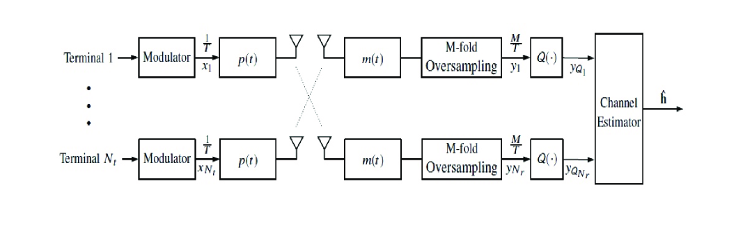
Fig. 1: System model of 1-bit multi-user multiple-antenna system with oversampling at the receiver

2 System Model

Consider the uplink of a single-cell multi-user large-scale MIMO system, as shown in Fig. 1, where there are $N_{t}$ single-antenna terminals and the BS is equipped with $N_{r}$ receive antennas. For the large-scale MIMO system we have $N_{r}\gg N_{t}$. The received oversampled signal $\mathbf{y}$ is

$$\mathbf{y}=\mathbf{H}\mathbf{x}+\mathbf{n},$$ (1)

where $\mathbf{x}\in\mathbb{C}^{NN_{t}\times 1}$ contains $N$ blocks of transmitted symbols. Each symbol is generated by independent and identically distributed (i.i.d.) random variable with zero mean and unit variance. The vector $\mathbf{n}\in\mathbb{C}^{MN_{r}N\times 1}$ contains filtered oversampled noise samples expressed by

$$\mathbf{n}=\left(\mathbf{I}_{N_{r}}\otimes\mathbf{G}\right)\mathbf{w}.$$ (2)

The entries of $\mathbf{w}$ are zero-mean i.i.d. complex Gaussian random variables, which we denote by $\mathcal{CN}\left(\mathbf{0}_{3MN_{r}N},\sigma^{2}_{n}\mathbf{I}_{3MN_{r}N}\right)$. Since the receive filter length is $2MN+1$, more samples (e.g. $3MN$) in $\mathbf{w}$ need to be considered to have the same statistical property of each entry in $\mathbf{n}$. $\mathbf{G}$ is a Toeplitz matrix described by (3), which contains the coefficients of the matched filter $m(t)$ at different time instants,

$$\mathbf{G}=\begin{bmatrix}m(-NT)&m(-NT+\frac{1}{M}T)&\dots&m(NT)&0&\dots&0\\ 0&m(-NT)&\dots&m(NT-\frac{1}{M}T)&m(NT)&\dots&0\\ \vdots&\vdots&\ddots&\vdots&\vdots&\ddots&\vdots\\ 0&0&\dots&m(-NT)&m(-NT+\frac{1}{M}T)&\dots&m(NT)\\ \end{bmatrix}_{MN\times 3MN}$$ (3)

where the symbol period is represented by $T$.

The equivalent channel matrix $\mathbf{H}\in\mathbb{C}^{MN_{r}N\times NN_{t}}$ is described as

$$\mathbf{H}=\left(\mathbf{I}_{N_{r}}\otimes\mathbf{Z}\right)\mathbf{U}\left(\mathbf{H}^{\prime}\otimes\mathbf{I}_{N}\right),$$ (4)

where $\mathbf{H}^{\prime}\in\mathbb{C}^{N_{r}\times N_{t}}$ is the channel matrix for the non-oversampled systems and $\mathbf{U}$ is the oversampling matrix described by

$$\mathbf{U}=\mathbf{I}_{N_{r}N}\otimes\mathbf{u}=\mathbf{I}_{N_{r}N}\otimes\left[0\quad\cdots\quad 0\quad 1\right]^{T}_{1\times M}.$$ (5)

$\mathbf{Z}\in\mathbb{R}^{MN\times MN}$ is a Toeplitz matrix with the form

$$\leavevmode\resizebox{232.97455pt}{}{$\displaystyle\mathbf{Z}=\begin{bmatrix}z(0)&z(\frac{T}{M})&\dots&z(NT-\frac{1}{M}T)\\ z(-\frac{T}{M})&z(0)&\dots&z(NT-\frac{2}{M}T)\\ \vdots&\vdots&\ddots&\vdots\\ z(-NT+\frac{1}{M}T)&z(-NT+\frac{2}{M}T)&\dots&z(0)\\ \end{bmatrix}$},$$ (6)

where $z(t)$ is the convolution of the pulse shaping filter $p(t)$ and the matched filter $m(t)$. In particular, $M=1$ refers to the non-oversampling case.

Let $\mathcal{Q}(.)$ represent the 1-bit quantization function, the received quantized signal $\mathbf{y}_{\mathcal{Q}}$ is

$$\mathbf{y}_{\mathcal{Q}}=\frac{1}{\sqrt{2}}\mathcal{Q}\left(\mathbf{y}\right)=\frac{1}{\sqrt{2}}\mathcal{Q}\left(\mathbf{y}^{R}\right)+j\frac{1}{\sqrt{2}}\mathcal{Q}\left(\mathbf{y}^{I}\right),$$ (7)

The real and imaginary parts are element-wisely quantized to $\{\pm 1\}$ based on the sign, respectively.

3 Fisher Information and Channel Estimation for 1-bit MIMO

This section firstly analyzes the FI about the unknown channel parameters and gives deterministic CRBs on the variance of any unbiased channel estimator for both non-oversampled and oversampled 1-bit MIMO systems. The proposed LRA-LS channel estimator and the adaptive estimation of the autocorrelation matrix of the channel vector is then described in the last part.

The system model in (1) can be vectorized as

$$\mathbf{y} =(\mathbf{x}^{T}\otimes\mathbf{I}_{N_{r}NM})\text{vec}(\mathbf{H})+\mathbf{n}$$ (8)

$$=[\mathbf{x}^{T}\otimes\mathbf{I}_{N_{r}}\otimes\mathbf{Z}(\mathbf{I}_{N}\otimes\mathbf{u})]\text{vec}(\mathbf{H}^{\prime}\otimes\mathbf{I}_{N})+\mathbf{n}$$

with the property of vectorization and Kronecker products

$$\text{vec}(\mathbf{H}^{\prime}\otimes\mathbf{I}_{N}) =$$ (9)

$$\left[\mathbf{I}_{N_{t}}\otimes\left(\mathbf{e}_{1}\otimes\mathbf{I}_{N_{r}}\otimes\mathbf{e}_{1}+\dots+\mathbf{e}_{N}\otimes\mathbf{I}_{N_{r}}\otimes\mathbf{e}_{N}\right)\right]\text{vec}(\mathbf{H^{\prime}}),$$

where $\mathbf{e}_{n}$ is an all zeros column vector except that the $n$th element is one. Eq.(8) can be written in the following simplified form

$$\mathbf{y}=\mathbf{\Phi}\text{vec}(\mathbf{H^{\prime}})+\mathbf{n}=\mathbf{\Phi}\mathbf{h}^{\prime}+\mathbf{n},$$ (10)

where $\mathbf{\Phi}\in\mathbb{C}^{MNN_{r}\times N_{r}N_{t}}$ is called the equivalent transmit matrix.

To calculate the FI, we rewrite (10) in the real-valued form as

$$\begin{bmatrix}\mathbf{y}^{R}\\ \mathbf{y}^{I}\end{bmatrix}=\begin{bmatrix}\mathbf{\Phi}^{R}&-\mathbf{\Phi}^{I}\\ \mathbf{\Phi}^{I}&\mathbf{\Phi}^{R}\end{bmatrix}\begin{bmatrix}\mathbf{h^{\prime}}^{R}\\ \mathbf{h^{\prime}}^{I}\end{bmatrix}+\begin{bmatrix}\mathbf{n}^{R}\\ \mathbf{n}^{I}\end{bmatrix}.$$ (11)

Considering the unknown parameter vector $\tilde{\mathbf{h^{\prime}}}=[\mathbf{h^{\prime}}^{R};\mathbf{h^{\prime}}^{I}]$ and with the independence of $\mathbf{y}^{R}$ and $\mathbf{y}^{I}$, the FI matrix [19] of the quantized signal is defined as

$$\mathbf{F}_{\mathbf{y}_{\mathcal{Q}}}(\tilde{\mathbf{h^{\prime}}})=\mathbf{F}_{\mathbf{y}_{\mathcal{Q}}^{R}}(\tilde{\mathbf{h^{\prime}}})+\mathbf{F}_{\mathbf{y}_{\mathcal{Q}}^{I}}(\tilde{\mathbf{h^{\prime}}}),$$ (12)

where

$$[\mathbf{F}_{\mathbf{y}_{\mathcal{Q}}^{R/I}}(\tilde{\mathbf{h^{\prime}}})]_{ij}=E_{\mathbf{y}_{\mathcal{Q}}^{R/I}\mid\tilde{\mathbf{h^{\prime}}}}\left\{\frac{\partial\ln p(\mathbf{y}_{\mathcal{Q}}^{R/I}\mid\tilde{\mathbf{h^{\prime}}})}{\partial[\tilde{\mathbf{h^{\prime}}}]_{i}}\frac{\partial\ln p(\mathbf{y}_{\mathcal{Q}}^{R/I}\mid\tilde{\mathbf{h^{\prime}}})}{\partial[\tilde{\mathbf{h^{\prime}}}]_{j}}\right\}$$ (13)

with $[\tilde{\mathbf{h^{\prime}}}]_{i}$ and $[\tilde{\mathbf{h^{\prime}}}]_{j}$ being the elements of $\tilde{\mathbf{h^{\prime}}}$. The variance of any unbiased estimator $\hat{\tilde{\mathbf{h^{\prime}}}}$ is lower bounded by

$$\text{var}\{[\hat{\tilde{\mathbf{h^{\prime}}}}]_{i}\}\geq[\mathbf{F}_{\mathbf{y}_{\mathcal{Q}}}^{-1}(\tilde{\mathbf{h^{\prime}}})]_{ii}.$$ (14)

3.1 Fisher Information for Non-oversampled Systems

For non-oversampled system, i.e, $M=1$, the noise vector $\mathbf{n}$ contains white Gaussian noise samples with covariance matrix $\mathbf{C}_{\mathbf{n}}=\sigma_{n}^{2}\mathbf{I}_{NN_{r}}$. The log-likelihood function can be expressed as

$$\ln p(\mathbf{y}_{\mathcal{Q}}\mid\tilde{\mathbf{h^{\prime}}})=\sum_{k=1}^{NN_{r}}\left[\ln p([\mathbf{y}_{\mathcal{Q}}^{R}]_{k}\mid\tilde{\mathbf{h^{\prime}}})+\ln p([\mathbf{y}_{\mathcal{Q}}^{I}]_{k}\mid\tilde{\mathbf{h^{\prime}}})\right]$$ (15)

with

$$p\left([\mathbf{y}_{\mathcal{Q}}^{R}]_{k}=\frac{1}{\sqrt{2}}\mid\tilde{\mathbf{h^{\prime}}}\right)=Q\left(-\frac{[\mathbf{\Phi}^{R}\mathbf{h^{\prime}}^{R}-\mathbf{\Phi}^{I}\mathbf{h^{\prime}}^{I}]_{k}}{\sigma_{n}/\sqrt{2}}\right)$$ (16)

$$p\left([\mathbf{y}_{\mathcal{Q}}^{R}]_{k}=-\frac{1}{\sqrt{2}}\mid\tilde{\mathbf{h^{\prime}}}\right)=Q\left(\frac{[\mathbf{\Phi}^{R}\mathbf{h^{\prime}}^{R}-\mathbf{\Phi}^{I}\mathbf{h^{\prime}}^{I}]_{k}}{\sigma_{n}/\sqrt{2}}\right)$$ (17)

$$p\left([\mathbf{y}_{\mathcal{Q}}^{I}]_{k}=\frac{1}{\sqrt{2}}\mid\tilde{\mathbf{h^{\prime}}}\right)=Q\left(-\frac{[\mathbf{\Phi}^{I}\mathbf{h^{\prime}}^{R}+\mathbf{\Phi}^{R}\mathbf{h^{\prime}}^{I}]_{k}}{\sigma_{n}/\sqrt{2}}\right)$$ (18)

$$p\left([\mathbf{y}_{\mathcal{Q}}^{I}]_{k}=-\frac{1}{\sqrt{2}}\mid\tilde{\mathbf{h^{\prime}}}\right)=Q\left(\frac{[\mathbf{\Phi}^{I}\mathbf{h^{\prime}}^{R}+\mathbf{\Phi}^{R}\mathbf{h^{\prime}}^{I}]_{k}}{\sigma_{n}/\sqrt{2}}\right),$$ (19)

where $Q(x)=\frac{1}{\sqrt{2\pi}}\int_{x}^{\infty}\exp(-\frac{u^{2}}{2})du$. With the derivative of $Q(x)$ function, the FI for the real part is given by

_ij $$=\sum_{k=1}^{NN_{r}}-E\left\{\frac{\partial^{2}\ln p([\mathbf{y}_{\mathcal{Q}}^{R}]_{k}\mid\tilde{\mathbf{h^{\prime}}})}{\partial[\tilde{\mathbf{h^{\prime}}}]_{i}\partial[\tilde{\mathbf{h^{\prime}}}]_{j}}\right\}$$ (20)

$$=\frac{1}{\pi\sigma_{n}^{2}}\sum_{k=1}^{NN_{r}}\frac{\exp(-\frac{[\mathbf{\Phi}^{R}\mathbf{h^{\prime}}^{R}-\mathbf{\Phi}^{I}\mathbf{h^{\prime}}^{I}]_{k}^{2}}{\sigma_{n}^{2}/2})\frac{\partial[\mathbf{\Phi}^{R}\mathbf{h^{\prime}}^{R}-\mathbf{\Phi}^{I}\mathbf{h^{\prime}}^{I}]_{k}}{\partial[\tilde{\mathbf{h^{\prime}}}]_{i}}\frac{\partial[\mathbf{\Phi}^{R}\mathbf{h^{\prime}}^{R}-\mathbf{\Phi}^{I}\mathbf{h^{\prime}}^{I}]_{k}}{\partial[\tilde{\mathbf{h^{\prime}}}]_{j}}}{Q\left(\frac{[\mathbf{\Phi}^{R}\mathbf{h^{\prime}}^{R}-\mathbf{\Phi}^{I}\mathbf{h^{\prime}}^{I}]_{k}}{\sigma_{n}/\sqrt{2}}\right)Q\left(-\frac{[\mathbf{\Phi}^{R}\mathbf{h^{\prime}}^{R}-\mathbf{\Phi}^{I}\mathbf{h^{\prime}}^{I}]_{k}}{\sigma_{n}/\sqrt{2}}\right)}.$$

The derivation for the imaginary part is analogous.

3.2 Fisher Information for Oversampled Systems

When $M\geq 2$ the equivalent noise vector $\mathbf{n}$ contains correlated noise samples. Computing the exact form of $p(\mathbf{y}_{\mathcal{Q}}^{R/I}\mid\tilde{\mathbf{h^{\prime}}})$ is not available or it is too difficult to compute. Instead, the authors in [20] have given a lower bound of the FI, which is based on the first and second order moments

$$\mathbf{F}_{\mathbf{y}_{\mathcal{Q}}^{R/I}}(\tilde{\mathbf{h^{\prime}}})\geq\left(\frac{\partial\mathbf{\mu}_{\mathbf{y}_{\mathcal{Q}}^{R/I}}}{\partial\tilde{\mathbf{h^{\prime}}}}\right)^{T}\mathbf{C}^{-1}_{\mathbf{y}^{R/I}_{\mathcal{Q}}}\left(\frac{\partial\mathbf{\mu}_{\mathbf{y}_{\mathcal{Q}}^{R/I}}}{\partial\tilde{\mathbf{h^{\prime}}}}\right)=\tilde{\mathbf{F}}_{\mathbf{y}_{\mathcal{Q}}^{R/I}}(\tilde{\mathbf{h^{\prime}}}),$$ (21)

where the equality holds for $M=1$. Since the lower-bounding technique is identical for the real and the imaginary part, we present only the derivation of $\tilde{\mathbf{F}}_{\mathbf{y}_{\mathcal{Q}}^{R}}(\tilde{\mathbf{h^{\prime}}})$. Based on [21], the mean value of the $k$th received symbol is given by

_k $$=\frac{1}{\sqrt{2}}P\left([\mathbf{y}_{\mathcal{Q}}^{R}]_{k}=+1\mid\tilde{\mathbf{h^{\prime}}}\right)-\frac{1}{\sqrt{2}}P\left([\mathbf{y}_{\mathcal{Q}}^{R}]_{k}=-1\mid\tilde{\mathbf{h^{\prime}}}\right)$$ (22)

$$=\frac{1}{\sqrt{2}}\left[1-2Q\left(\frac{[\mathbf{\Phi}^{R}\mathbf{h^{\prime}}^{R}-\mathbf{\Phi}^{I}\mathbf{h^{\prime}}^{I}]_{k}}{\sqrt{[\mathbf{C}_{\mathbf{n}}]_{kk}/2}}\right)\right],$$

The derivative of (22) is

$$\frac{\partial[\mathbf{\mu}_{\mathbf{y}_{\mathcal{Q}}^{R}}]_{k}}{\partial[\tilde{\mathbf{h^{\prime}}}]_{i}}=\frac{2\text{exp}\left(-\frac{[\mathbf{\Phi}^{R}\mathbf{h^{\prime}}^{R}-\mathbf{\Phi}^{I}\mathbf{h^{\prime}}^{I}]_{k}^{2}}{[\mathbf{C}_{\mathbf{n}}]_{kk}}\right)\frac{\partial[\mathbf{\Phi}^{R}\mathbf{h^{\prime}}^{R}-\mathbf{\Phi}^{I}\mathbf{h^{\prime}}^{I}]_{k}}{\partial[\tilde{\mathbf{h^{\prime}}}]_{i}}}{\sqrt{2\pi[\mathbf{C}_{\mathbf{n}}]_{kk}}}.$$ (23)

The diagonal elements of the covariance matrix are given by

$$[\mathbf{C}_{\mathbf{y}^{R}_{\mathcal{Q}}}]_{kk}=\frac{1}{2}-[\mathbf{\mu}_{\mathbf{y}_{\mathcal{Q}}^{R}}]_{k}^{2},$$ (24)

while the off-diagonal elements are calculated as

$${}_{kn}= P(z_{k}>0,z_{n}>0)+P(z_{k}\leq 0,z_{n}\leq 0)$$ (25)

$$-\frac{1}{2}-[\mathbf{\mu}_{\mathbf{y}_{\mathcal{Q}}^{R}}]_{k}[\mathbf{\mu}_{\mathbf{y}_{\mathcal{Q}}^{R}}]_{n},$$

where $[z_{k},z_{n}]^{T}$ is a bi-variate Gaussian random vector

$$\begin{bmatrix}z_{k}\\ z_{n}\end{bmatrix}\sim\mathcal{N}\left(\begin{bmatrix}[\mathbf{\Phi}^{R}\mathbf{h^{\prime}}^{R}-\mathbf{\Phi}^{I}\mathbf{h^{\prime}}^{I}]_{k}\\ [\mathbf{\Phi}^{R}\mathbf{h^{\prime}}^{R}-\mathbf{\Phi}^{I}\mathbf{h^{\prime}}^{I}]_{n}\end{bmatrix},\frac{1}{2}\begin{bmatrix}[\mathbf{C}_{\mathbf{n}}]_{kk}&[\mathbf{C}_{\mathbf{n}}]_{kn}\\ [\mathbf{C}_{\mathbf{n}}]_{nk}&[\mathbf{C}_{\mathbf{n}}]_{nn}\end{bmatrix}\right).$$

The lower bound for the imaginary part is derived in the same way.

3.3 Oversampling based LRA-LS Channel Estimation

In each uplink transmission block pilots are located before the data symbols. During the training phase, all terminals simultaneously transmit $\tau$ pilot sequences to the BS. Eq.(10) yields

$$\mathbf{y}_{p}=\mathbf{\Phi}_{p}\mathbf{h^{\prime}}+\mathbf{n}_{p}.$$ (26)

In particular, for the 1-bit quantization and with the Bussgang theorem (26) can be decomposed as

$$\mathbf{y}_{\mathcal{Q}_{p}}=\mathcal{Q}(\mathbf{\Phi}_{p}\mathbf{h^{\prime}}+\mathbf{n}_{p})=\tilde{\mathbf{\Phi}}_{p}\mathbf{h^{\prime}}+\tilde{\mathbf{n}}_{p},$$ (27)

where $\tilde{\mathbf{\Phi}}_{p}\in\mathbb{C}^{M\tau N_{r}\times N_{t}N_{r}}=\mathbf{A}_{p}\mathbf{\Phi}_{p}$ and $\tilde{\mathbf{n}}_{p}\in\mathbb{C}^{M\tau N_{r}\times 1}=\mathbf{A}_{p}\mathbf{n}_{p}+\mathbf{n}_{q}$. The vector $\mathbf{n}_{q}$ is the statistically equivalent quantizer noise. The matrix $\mathbf{A}_{p}\in\mathbb{R}^{M\tau N_{r}\times M\tau N_{r}}$ is the linear operator chosen independently from $\mathbf{y}_{p}$, which yields

$$\mathbf{A}_{p}=\mathbf{C}_{\mathbf{y}_{p}\mathbf{y}_{\mathcal{Q}_{p}}}^{H}\mathbf{C}_{\mathbf{y}_{p}}^{-1}=\sqrt{\frac{2}{\pi}}\text{diag}\left(\mathbf{C}_{\mathbf{y}_{p}}\right)^{-\frac{1}{2}},$$ (28)

where $\mathbf{C}_{\mathbf{y}_{p}\mathbf{y}_{\mathcal{Q}_{p}}}$ denotes the cross-correlation matrix between the received signal $\mathbf{y}_{p}$ and the quantized signal $\mathbf{y}_{\mathcal{Q}_{p}}$ [22]

$$\mathbf{C}_{\mathbf{y}_{p}\mathbf{y}_{\mathcal{Q}_{p}}}=\sqrt{\frac{2}{\pi}}\text{diag}(\mathbf{C}_{\mathbf{y}_{p}})^{-\frac{1}{2}}\mathbf{C}_{\mathbf{y}_{p}}.$$ (29)

$\mathbf{C}_{\mathbf{y}_{p}}$ is the auto-correlation matrix of $\mathbf{y}_{p}$, as follows:

$$\mathbf{C}_{\mathbf{y}_{p}}=\mathbf{\Phi}_{p}\mathbf{R}_{\mathbf{h^{\prime}}}\mathbf{\Phi}_{p}^{H}+\sigma_{n}^{2}\left(\mathbf{I}_{N_{r}}\otimes\mathbf{GG}^{H}\right).$$ (30)

Based on the equivalent linear model (27), the LS estimate of $\mathbf{h^{\prime}}$ is given by

$$\hat{\mathbf{h^{\prime}}}_{LS} =\operatorname*{arg\,min}_{\bar{\mathbf{h^{\prime}}}}\quad(\mathbf{y}_{\mathcal{Q}_{p}}-\tilde{\mathbf{\Phi}}_{p}\bar{\mathbf{h^{\prime}}})^{H}(\mathbf{y}_{\mathcal{Q}_{p}}-\tilde{\mathbf{\Phi}}_{p}\bar{\mathbf{h^{\prime}}})$$ (31)

$$=(\tilde{\mathbf{\Phi}}_{p}^{H}\tilde{\mathbf{\Phi}}_{p})^{-1}\tilde{\mathbf{\Phi}}_{p}^{H}\mathbf{y}_{\mathcal{Q}_{p}}.$$

In practice, $\mathbf{R}_{\mathbf{h^{\prime}}}=E\{\mathbf{h^{\prime}}\mathbf{h^{\prime}}^{H}\}$ is not known at the receiver, which is a limitation for the BLMMSE channel estimator. We propose an adaptive technique to recursively estimate it as

$$\hat{\mathbf{R}}_{\mathbf{h^{\prime}}}[n+1]=\lambda\hat{\mathbf{R}}_{\mathbf{h^{\prime}}}[n]+\hat{\mathbf{h^{\prime}}}[n]\hat{\mathbf{h^{\prime}}}[n]^{H},\quad 1\leq n\leq\tau,$$ (32)

where $\lambda$ is the forgetting factor and $\hat{\mathbf{h^{\prime}}}[n]$ is the channel estimate at time instant n. Consider the system model

$$\mathbf{y}_{\mathcal{Q}}[n] =\mathcal{Q}(\mathbf{H}\mathbf{x}[n]+\mathbf{n}[n])$$ (33)

$$=\mathcal{Q}\left((\mathbf{x}^{T}[n]\otimes\mathbf{I}_{N_{r}}\otimes\mathbf{Z^{\prime}u})\mathbf{h^{\prime}}+\mathbf{n}[n]\right),$$

where $\mathbf{y}_{\mathcal{Q}}[n]$, $\mathbf{x}[n]$ and $\mathbf{n}[n]$ are column vectors with size $MN_{r}\times 1$, $N_{t}\times 1$ and $MN_{r}\times 1$, respectively. $\mathbf{Z^{\prime}}\in\mathbb{R}^{M\times M}$ is a simplified version of $\mathbf{Z}$. The instantaneous estimate of $\mathbf{h^{\prime}}$ is calculated as

$$\hat{\mathbf{h^{\prime}}}[n]=\left(\mathbf{x}^{T}[n]\otimes\mathbf{I}_{N_{r}}\otimes\mathbf{Z^{\prime}u}\right)^{+}\mathbf{y}_{\mathcal{Q}}[n].$$ (34)

The initial guess of $\hat{\mathbf{R}}_{\mathbf{h^{\prime}}}[1]$ is an all-zeros matrix. Note that the proposed LRA-LS channel estimator is a biased estimator. While calculating the Cramér-Rao upper bound, it should apply as follows

$$\frac{\partial E\{\hat{\tilde{\mathbf{h^{\prime}}}}_{LS}\}}{\partial\tilde{\mathbf{h^{\prime}}}}\left(\tilde{\mathbf{F}}_{\mathbf{y}_{\mathcal{Q}}}^{-1}(\tilde{\mathbf{h^{\prime}}})\frac{\partial E\{\hat{\tilde{\mathbf{h^{\prime}}}}_{LS}\}}{\partial\tilde{\mathbf{h^{\prime}}}}\right)^{T}.$$ (35)

Instead of directly calculating the gradient of expectation with respect to the channel vector, we numerically evaluate this gradient, since there is an adaptive estimation technique inside the channel estimator. Other estimators [23, 24, 25] can also be considered.

4 Numerical Results

This section presents simulation results of the proposed oversampling based LRA-LS channel estimation algorithm. We have used QPSK as the modulation scheme. The $m(t)$ and $p(t)$ filters are normalized Root-Raised-Cosine (RRC) filters with a roll-off factor of 0.8. The channel is assumed to experience block fading and $\mathbf{C}_{\mathbf{h^{\prime}}}=\mathbf{I}_{N_{r}N_{t}}$. The forgetting factor $\lambda$ is set to 0.91. The pilot sequences are orthogonal. The signal-to-noise ratio (SNR) is defined as $10\log(\frac{N_{t}}{\sigma_{n}^{2}})$. Fig. 2 shows the normalized mean square error (NMSE) performance of the proposed channel estimator and the analytical upper bound of CRB. When using the LRA-LS channel estimator, there is a 2 dB performance gain of the oversampled system ($M=2$ or 3) compared to the non-oversampled system ($M=1$). The upper bound of CRB is calculated based on the corresponding lower bound of FI. Fig. 3 shows the NMSE performances of the system with different lengths of pilot symbols at SNR=0dB, where the proposed channel estimator approaches the performance of the upper bound of CRB.

In the simulations we have chosen $\tau=40$ as the trade-off between system complexity and estimation performance. The symbol error rate (SER) performances of the oversampled system with estimated CSI (channel state information) and perfect CSI are shown in Fig. 3, where the sliding window based linear receiver with window length 3 [26] is applied in the system. Other detection schemes [27, 28, 29, 30, 31] can also be considered.

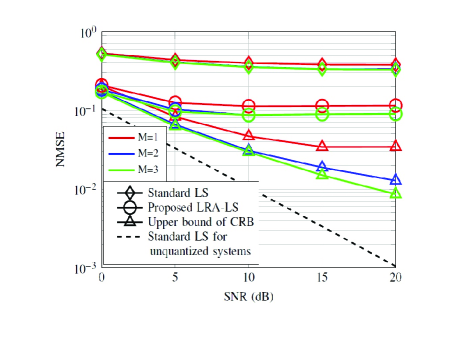
Fig. 2: $N_{t}=4$ and $N_{r}=16$. NMSE comparison between different oversampling factors with $\tau=40$.

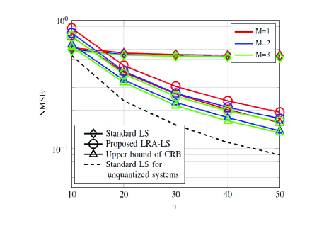
Fig. 3: $N_{t}=4$ and $N_{r}=16$. NMSE comparison as a function of pilot length when $\text{SNR}=0\text{dB}$.

5 Conclusion

This work has proposed the LRA-LS channel estimator for uplink large-scale MIMO systems with 1-bit quantization and oversampling at the receiver. We have further given analytical performance of the system in terms of the FI. For the non-oversampled system, the equivalent noise vector $\mathbf{n}$ contains white noise samples and the lower bound of FI is the same as the actual FI. The simulation results have shown that the proposed channel estimator in oversampled systems achieves better performance than that of non-oversampled systems. $\mathcal{F}$

References

• [1] E. G. Larsson, O. Edfors, F. Tufvesson, and T. L. Marzetta, “Massive MIMO for next generation wireless systems,” IEEE Commun. Mag., vol. 52, no. 2, pp. 186–195, Feb. 2014.
• [2] R. C. de Lamare, “Massive mimo systems: Signal processing challenges and future trends,” URSI Radio Science Bulletin, vol. 2013, no. 347, pp. 8–20, Dec 2013.
• [3] H. Q. Ngo, E. G. Larsson, and T. L. Marzetta, “Energy and spectral efficiency of very large multiuser mimo systems,” IEEE Transactions on Communications, vol. 61, no. 4, pp. 1436–1449, Apr. 2013.
• [4] W. Zhang, H. Ren, C. Pan, M. Chen, R. C. de Lamare, B. Du, and J. Dai, “Large-scale antenna systems with ul/dl hardware mismatch: Achievable rates analysis and calibration,” IEEE Transactions on Communications, vol. 63, no. 4, pp. 1216–1229, April 2015.
• [5] F. Rusek, D. Persson, B. K. Lau, E. G. Larsson, T. L. Marzetta, O. Edfors, and F. Tufvesson, “Scaling Up MIMO: Opportunities and Challenges with Very Large Arrays,” IEEE Signal Process. Mag., vol. 30, no. 1, pp. 40–60, Jan. 2013.
• [6] S. Jacobsson, G. Durisi, M. Coldrey, U. Gustavsson, and C. Studer, “Throughput Analysis of Massive MIMO Uplink With Low-Resolution ADCs,” IEEE Trans. Wireless Commun., vol. 16, no. 6, pp. 4038–4051, Jun. 2017.
• [7] C. Studer and G. Durisi, “Quantized Massive MU-MIMO-OFDM Uplink,” IEEE Trans. Commun., vol. 64, no. 6, pp. 2387–2399, Jun. 2016.
• [8] S. Wang, Y. Li, and J. Wang, “Multiuser Detection in Massive Spatial Modulation MIMO With Low-Resolution ADCs,” IEEE Trans. Wireless Commun., vol. 14, no. 4, pp. 2156–2168, Apr. 2015.
• [9] L. T. N. Landau, M. Dorpinghaus, R. C. de Lamare, and G. P. Fettweis, “Achievable rate with 1-bit quantization and oversampling using continuous phase modulation-based sequences,” IEEE Transactions on Wireless Communications, vol. 17, no. 10, pp. 7080–7095, Oct 2018.
• [10] J. Zhang, L. Dai, X. Li, Y. Liu, and L. Hanzo, “On Low-Resolution ADCs in Practical 5G Millimeter-Wave Massive MIMO Systems,” IEEE Commun. Mag., vol. 56, no. 7, pp. 205–211, Jul. 2018.
• [11] J. Mo, P. Schniter, N. G. Prelcic, and R. W. Heath, “Channel estimation in millimeter wave MIMO systems with one-bit quantization,” in 2014 48th Asilomar Conference on Signals, Systems and Computers, Nov. 2014, pp. 957–961.
• [12] J. Mo and R. W. Heath, “High SNR capacity of millimeter wave MIMO systems with one-bit quantization,” in 2014 Information Theory and Applications Workshop (ITA), Feb. 2014, pp. 1–5.
• [13] Z. Shao, L. T. N. Landau, and R. C. de Lamare, “Channel estimation using 1-bit quantization and oversampling for large-scale multiple-antenna systems,” in ICASSP 2019 - 2019 IEEE International Conference on Acoustics, Speech and Signal Processing (ICASSP), May 2019, pp. 4669–4673.
• [14] L. T. N. Landau and R. C. de Lamare, “Branch-and-Bound Precoding for Multiuser MIMO Systems With 1-Bit Quantization,” IEEE Wireless Commun. Lett., vol. 6, no. 6, pp. 770–773, Dec. 2017.
• [15] Z. Shao, L. Landau, and R. C. de Lamare, “Adaptive RLS Channel Estimation and SIC for Large-Scale Antenna Systems with 1-Bit ADCs,” in WSA 2018; 22nd International ITG Workshop on Smart Antennas, Mar. 2018, pp. 1–4.
• [16] J. Mo and R. W. Heath, “Capacity Analysis of One-Bit Quantized MIMO Systems With Transmitter Channel State Information,” IEEE Trans. Signal Process., vol. 63, no. 20, pp. 5498–5512, Oct. 2015.
• [17] Z. Shao, R. C. de Lamare, and L. T. N. Landau, “Iterative Detection and Decoding for Large-Scale Multiple-Antenna Systems With 1-Bit ADCs,” IEEE Wireless Commun. Lett., vol. 7, no. 3, pp. 476–479, Jun. 2018.
• [18] A. B. Üçüncü and A. Ö. Yılmaz, “Oversampling in one-bit quantized massive mimo systems and performance analysis,” IEEE Trans. Wireless Commun., pp. 1–1, 2018.
• [19] Steven M. Kay, Fundamentals of Statistical Signal Processing: Estimation Theory, Prentice-Hall, Inc., Upper Saddle River, NJ, USA, 1993.
• [20] M. Stein, A. Mezghani, and J. A. Nossek, “A Lower Bound for the Fisher Information Measure,” IEEE Signal Process. Lett., vol. 21, no. 7, pp. 796–799, Jul. 2014.
• [21] M. Schlüter, M. Dörpinghaus, and G. P. Fettweis, “Bounds on Channel Parameter Estimation with 1-Bit Quantization and Oversampling,” in 2018 IEEE 19th International Workshop on Signal Processing Advances in Wireless Communications (SPAWC), Jun. 2018, pp. 1–5.
• [22] J. J. Bussgang, “Crosscorrelation functions of amplitude-distorted Gaussian signals,” Res. Lab. Elec., Mas. Inst. Technol., vol. Tech. Rep. 216, Mar. 1952.
• [23] R. C. de Lamare and R. Sampaio-Neto, “Reduced-rank adaptive filtering based on joint iterative optimization of adaptive filters,” IEEE Signal Processing Letters, vol. 14, no. 12, pp. 980–983, Dec 2007.
• [24] R. C. de Lamare and R. Sampaio-Neto, “Adaptive reduced-rank processing based on joint and iterative interpolation, decimation, and filtering,” IEEE Transactions on Signal Processing, vol. 57, no. 7, pp. 2503–2514, July 2009.
• [25] R. C. de Lamare and R. Sampaio-Neto, “Adaptive reduced-rank equalization algorithms based on alternating optimization design techniques for mimo systems,” IEEE Transactions on Vehicular Technology, vol. 60, no. 6, pp. 2482–2494, July 2011.
• [26] Z. Shao, L. T. N. Landau, and R. C. de Lamare, “Sliding Window Based Linear Signal Detection Using 1-Bit Quantization and Oversampling for Large-Scale Multiple-Antenna Systems,” in 2018 IEEE Statistical Signal Processing Workshop (SSP), Jun. 2018, pp. 183–187.
• [27] R. C. De Lamare and R. Sampaio-Neto, “Minimum mean-squared error iterative successive parallel arbitrated decision feedback detectors for ds-cdma systems,” IEEE Transactions on Communications, vol. 56, no. 5, pp. 778–789, May 2008.
• [28] P. Li, R. C. de Lamare, and R. Fa, “Multiple feedback successive interference cancellation detection for multiuser mimo systems,” IEEE Transactions on Wireless Communications, vol. 10, no. 8, pp. 2434–2439, August 2011.
• [29] R. Fa and R. C. de Lamare, “Multi-branch successive interference cancellation for mimo spatial multiplexing systems: Design, analysis and adaptive implementation,” IET Communications, vol. 5, no. 4, pp. 484–494, March 2011.
• [30] P. Li and R. C. De Lamare, “Adaptive decision-feedback detection with constellation constraints for mimo systems,” IEEE Transactions on Vehicular Technology, vol. 61, no. 2, pp. 853–859, Feb 2012.
• [31] R. C. de Lamare, “Adaptive and iterative multi-branch mmse decision feedback detection algorithms for multi-antenna systems,” IEEE Transactions on Wireless Communications, vol. 12, no. 10, pp. 5294–5308, October 2013.