Light-Quark Dipole Operators at LHC

Abstract

We study the effect of operators generating dipole couplings of the light quarks to electroweak gauge bosons on several observables at LHC. We start by demonstrating that the determination of the gauge boson self-couplings from electroweak diboson production at LHC is robust under the inclusion of those quark dipole operators even when let them totally unconstrained in the analysis. Conversely, we determine the bounds that the diboson data imposes on the light-quark dipole couplings and show that they represent a significant improvement over the limits arising from $Z$ and $W$ electroweak precision measurements. We also explore the sensitivity of the Drell-Yan cross section determination at LHC Run 1, and the results on resonance searches in high invariant-mass lepton pair production at Run 2 to further constrain the electroweak dipole couplings of the light quarks.

I Introduction

The CERN Large Hadron Collider (LHC) has provided us with invaluable information on the Standard Model (SM) such as the discovery of a Higgs boson Aad et al. (2012); Chatrchyan et al. (2012) with properties compatible with the simplest realization of electroweak symmetry breaking, as well as the apparent lack of new states in the available data. In the absence of additional low scale particles, we are compelled to describe possible deviations from the SM predictions through an effective field theory Weinberg (1979) containing an ordered series of higher–dimension operators built of the SM fields. In this context, and within the present experimental results, one can proceed under the assumption that the new operators are linearly invariant under the SM gauge group $SU(3)_{C}\otimes SU(2)_{L}\otimes U(1)_{Y}$ and we write

$${\cal L}_{\rm eff}={\cal L}_{\rm SM}+\sum_{n>4,j}\frac{f_{n,j}}{\Lambda^{n-4}}{\cal O}_{n,j}\;\;.$$ (1)

The first operators that impact the LHC physics are of $n=6$, i.e. dimension–six. The most general dimension-six operator basis respecting the SM gauge symmetry, as well as baryon and lepton number conservation, contains 59 independent operators, up to flavor and hermitian conjugation Buchmuller and Wyler (1986); Grzadkowski et al. (2010).

This work aims at studying the operators which generate dipole couplings of the light quarks to electroweak gauge bosons that belong to the dimension-six operator basis, focusing on their effects on several observables at LHC. In particular, it has been recently demonstrated that the electroweak gauge boson couplings to fermions can impact the LHC diboson analysis Zhang (2017); Baglio et al. (2017); Alves et al. (2018); da Silva Almeida et al. (2019) used to test the gauge boson self-interactions. Here, we extend the analysis of these events to study their sensitivity to the inclusion of light-quark electroweak dipole couplings. The aim is twofold. First, we want to test their possible effect on the extracted information on the gauge boson self-couplings. Second, we want to quantify the constraints that the analysis can impose on the Wilson coefficients of light-quark dipole operators. Moreover, we also explore the potential of Drell-Yan (DY) processes to further test these operators.

The light-quark electroweak dipole operators have been previously studied using electroweak precision data (EWPD) Escribano and Masso (1994); Kopp et al. (1995), as well as deep inelastic scattering results from HERA Kopp et al. (1995), leading to constraints on their Wilson coefficients of the order of $10$ TeV^-2. In the case of top quarks, the TopFitter collaboration Buckley et al. (2016) obtained limits on the corresponding operator coefficients ${\cal O}(12)$ TeV^-2 using LHC Run 2 data on the production of top quarks. Here, we show that the study of the diboson ($W^{+}W^{-}$, $W^{\pm}Z$) production at the LHC Run 1 and 2 leads to constraints on the Wilson coefficients of light-quark electroweak dipole operators that are an order of magnitude better than the ones stemming from the EWPD analysis. Moreover, we also show that Drell-Yan data can be used to further tighten the bounds on these operators.

II Theoretical Framework

In this work, we extend the SM, as in Eq. (1), by adding dimension-six operators that conserve $C$ and $P$, as well as lepton and baryon numbers. The basis of dimension-six operators is not unique due to the freedom associated to the use of he equations of motion (EOM) Politzer (1980); Georgi (1991); Arzt (1995); Simma (1994). Using that freedom we choose to work in the basis of Hagiwara, Ishihara, Szalapski, and Zeppenfeld (HISZ) Hagiwara et al. (1993, 1997) for the pure bosonic operators.

Our main focus is the study of operators containing electroweak dipole couplings for light quarks, which for simplicity we refer to as dipole operators in what follows. More specifically, these operators are

$$\begin{array}[]{l@{\hspace{1cm}}l@{\hspace{1cm}}l}{\cal O}_{uW,ij}=i\overline{Q}_{i}\sigma^{\mu\nu}u_{R,j}\widehat{W}_{\mu\nu}\tilde{\Phi}\;\;\;,\hfil\hskip 28.45274pt&{\cal O}_{uB,ij}=i\overline{Q}_{i}\sigma^{\mu\nu}u_{R,j}\widehat{B}_{\mu\nu}\tilde{\Phi}\;\;\;,\hfil\hskip 28.45274pt\\ {\cal O}_{dW,ij}=i\overline{Q}_{i}\sigma^{\mu\nu}d_{R,j}\widehat{W}_{\mu\nu}\Phi\;\;\;,\hfil\hskip 28.45274pt&{\cal O}_{dB,ij}=i\overline{Q}_{i}\sigma^{\mu\nu}u_{R,j}\widehat{B}_{\mu\nu}\Phi\;\;\;,\hfil\hskip 28.45274pt\end{array}$$ (2)

where $\Phi$ stands for the Higgs doublet and $\tilde{\Phi}=i\sigma_{2}\Phi^{*}$. We defined $\widehat{B}_{\mu\nu}\equiv i(g^{\prime}/2)B_{\mu\nu}$ and $\widehat{W}_{\mu\nu}\equiv i(g/2)\sigma^{a}W^{a}_{\mu\nu}$, with $g$ and $g^{\prime}$ being the $SU(2)_{L}$ and $U(1)_{Y}$ gauge couplings respectively, and $\sigma^{a}$ the Pauli matrices. $Q$ denotes the quark doublet and $f_{R}$ are the $SU(2)_{L}$ singlet fermions and $i$,$j$ are family indices.

For simplicity, we assume that the Wilson coefficient of the dipole operators are flavour diagonal and family independent, i.e. the dipole interactions are

$${\cal L}_{\rm eff}^{\rm DIP}=\frac{f_{uB}}{\Lambda^{2}}\sum_{i=1,2}{\cal O}_{uB,ii}+\frac{f_{uW}}{\Lambda^{2}}\sum_{i=1,2}{\cal O}_{uW,ii}+\frac{f_{dB}}{\Lambda^{2}}\sum_{i=1,2}{\cal O}_{uB,ii}+\frac{f_{dW}}{\Lambda^{2}}\sum_{i=1,2}{\cal O}_{uW,ii}+\hbox{h.c.}\;\;.$$ (3)

The effective interactions in Eq. (3) induce dipole-like couplings to photons, $Z$’s and $W^{\pm}$’s of the form

$${\cal L}=-\frac{e\,v}{\sqrt{2}}~{}\left[\frac{F_{f\gamma}}{\Lambda^{2}}\bar{f}\,\sigma^{\mu\nu}\,f\,\partial_{\mu}A_{\nu}\;+\;\frac{F_{fZ}}{\Lambda^{2}}\,\bar{f}\,\sigma^{\mu\nu}\,f\,\partial_{\mu}Z_{\nu}\right]-ev\left[\bar{f}\,\sigma^{\mu\nu}\left(\frac{F^{L}_{ff^{\prime}W}}{\Lambda^{2}}\,P_{L}\,+\frac{\,F^{R}_{ff^{\prime}W}}{\Lambda^{2}}\,P_{R}\right)\,f^{\prime}\,\partial_{\mu}W^{+}_{\nu}\;+\;{\rm h.c.}\right]$$ (4)

where $P_{L(R)}$ is the left- (right-)handed chiral projector and

$$\frac{F_{u\gamma}}{\Lambda^{2}}=\frac{f_{uW}}{\Lambda^{2}}+\frac{f_{uB}}{\Lambda^{2}}\;, \frac{F_{uZ}}{\Lambda^{2}}=\frac{c_{W}}{s_{W}}\frac{f_{uW}}{\Lambda^{2}}-\frac{s_{W}}{c_{W}}\frac{f_{uB}}{\Lambda^{2}}\;\;,$$

$$\frac{F_{d\gamma}}{\Lambda^{2}}=\frac{f_{dW}}{\Lambda^{2}}-\frac{f_{dB}}{\Lambda^{2}}\;\;, \frac{F_{dZ}}{\Lambda^{2}}=\frac{c_{W}}{s_{W}}\frac{f_{dW}}{\Lambda^{2}}+\frac{s_{W}}{c_{W}}\frac{f_{dB}}{\Lambda^{2}}\;,$$ (5)

$$\frac{F^{R}_{udW}}{\Lambda^{2}}=\frac{1}{s_{W}}\frac{f_{uW}}{\Lambda^{2}}\;\;, \frac{F^{L}_{udW}}{\Lambda^{2}}=\frac{1}{s_{W}}\frac{f_{dW}}{\Lambda^{2}}\;\;.$$

Here, $s_{W}$ ($c_{W}$) is the sine (cosine) of the weak mixing angle.

Consequently, the electroweak dipole operators contribute to any process at the LHC initiated by the quark and antiquark components of the colliding protons. In particular, they take part in electroweak diboson production $pp\rightarrow W^{+}W^{-}$ and $pp\rightarrow ZW^{\pm}$. Notwithstanding, there are further dimension-six operators that contribute to these processes like the following additional operators that change the couplings between gauge bosons and fermions

$$\begin{array}[]{l@{\hspace{1cm}}l@{\hspace{1cm}}l}\hfil\hskip 28.45274pt&{\cal O}^{(1)}_{\Phi L,ij}=\Phi^{\dagger}(i\,\mbox{$\raisebox{5.69054pt}{\boldmath${}^{\leftrightarrow}$}D$}_{\mu}\Phi)(\overline{L}_{i}\gamma^{\mu}L_{j})\;\;,\hfil\hskip 28.45274pt&{\cal O}^{(3)}_{\Phi L,ij}=\Phi^{\dagger}(i\,{\mbox{$\raisebox{5.69054pt}{\boldmath${}^{\leftrightarrow}$}D^{a}$}}_{\!\!\mu}\Phi)(\overline{L}_{i}\gamma^{\mu}T_{a}L_{j})\;\;,\\ \hfil\hskip 28.45274pt&\hfil\hskip 28.45274pt&\\ \hfil\hskip 28.45274pt&{\cal O}^{(1)}_{\Phi Q,ij}=\Phi^{\dagger}(i\,\mbox{$\raisebox{5.69054pt}{\boldmath${}^{\leftrightarrow}$}D$}_{\mu}\Phi)(\overline{Q}_{i}\gamma^{\mu}Q_{j})\;\;,\hfil\hskip 28.45274pt&{\cal O}^{(3)}_{\Phi Q,ij}=\Phi^{\dagger}(i\,{\mbox{$\raisebox{5.69054pt}{\boldmath${}^{\leftrightarrow}$}D^{a}$}}_{\!\!\mu}\Phi)(\overline{Q}_{i}\gamma^{\mu}T_{a}Q_{j})\;\;,\\ \hfil\hskip 28.45274pt&\hfil\hskip 28.45274pt&\\ \hfil\hskip 28.45274pt&{\cal O}^{(1)}_{\Phi u,ij}=\Phi^{\dagger}(i\,\mbox{$\raisebox{5.69054pt}{\boldmath${}^{\leftrightarrow}$}D$}_{\mu}\Phi)(\overline{u}_{R_{i}}\gamma^{\mu}u_{R_{j}})\;\;,\hfil\hskip 28.45274pt&{\cal O}^{(1)}_{\Phi d,ij}=\Phi^{\dagger}(i\,\mbox{$\raisebox{5.69054pt}{\boldmath${}^{\leftrightarrow}$}D$}_{\mu}\Phi)(\overline{d}_{R_{i}}\gamma^{\mu}d_{R_{j}})\;\;,\\ \hfil\hskip 28.45274pt&\hfil\hskip 28.45274pt&\\ \hfil\hskip 28.45274pt&{\cal O}^{(1)}_{\Phi e,ij}=\Phi^{\dagger}(i\mbox{$\raisebox{5.69054pt}{\boldmath${}^{\leftrightarrow}$}D$}_{\mu}\Phi)(\overline{e}_{R_{i}}\gamma^{\mu}e_{R_{j}})\;\;,\hfil\hskip 28.45274pt&{\cal O}^{(1)}_{\Phi ud}=\tilde{\Phi}^{\dagger}(i\,\mbox{$\raisebox{5.69054pt}{\boldmath${}^{\leftrightarrow}$}D$}_{\mu}\Phi)(\overline{u}_{R}\gamma^{\mu}d_{R}+{\rm h.c.})\;\;,\end{array}$$ (6)

where the lepton doublet (singlet) is denoted by $L$ ($e$) and we defined $\Phi^{\dagger}\mbox{$\raisebox{5.69054pt}{\boldmath${}^{\leftrightarrow}$}D$}_{\mu}\Phi=\Phi^{\dagger}D_{\mu}\Phi-(D_{\mu}\Phi)^{\dagger}\Phi$ and $\Phi^{\dagger}\mbox{$\raisebox{5.69054pt}{\boldmath${}^{\leftrightarrow}$}D^{a}$}_{\!\!\mu}\Phi=\Phi^{\dagger}T^{a}D_{\mu}\Phi-(D_{\mu}\Phi)^{\dagger}T^{a}\Phi$ with $T^{a}=\sigma^{a}/2$.

In addition to the above fermionic operators, diboson production also involves triple gauge couplings (TGC) which are directly modified by one operator that contains exclusively gauge bosons

$$\mathcal{O}_{WWW}={\rm Tr}[\widehat{W}_{\mu}^{\nu}\widehat{W}_{\nu}^{\rho}\widehat{W}_{\rho}^{\mu}]\;\;,$$ (7)

as well as, three additional dimension-six operators that include Higgs and electroweak gauge fields in the HISZ basis

$$\begin{array}[]{lllll}\mathcal{O}_{W}=(D_{\mu}\Phi)^{\dagger}\widehat{W}^{\mu\nu}(D_{\nu}\Phi)&\hbox{,}&\mathcal{O}_{B}=(D_{\mu}\Phi)^{\dagger}\widehat{B}^{\mu\nu}(D_{\nu}\Phi)&\hbox{and}&\mathcal{O}_{BW}=\Phi^{\dagger}\widehat{B}_{\mu\nu}\widehat{W}^{\mu\nu}\Phi\;\;.\end{array}$$ (8)

It is interesting to notice that, besides giving a direct contribution to TGC’s, $\mathcal{O}_{BW}$ also leads to a finite renormalization of the SM gauge fields, therefore, modifying the electroweak gauge-boson couplings. Furthermore, two other dimension-six operators also enter in our studies via finite renormalization effects, namely,

$${\cal O}_{LLLL}=(\overline{L}\gamma^{\mu}L)(\overline{L}\gamma^{\mu}L)\;\;\;\;\hbox{ and }\;\;\;\;\mathcal{O}_{\Phi,1}=(D_{\mu}\Phi)^{\dagger}\Phi\Phi^{\dagger}(D^{\mu}\Phi)\;\;.$$ (9)

In brief, ${\cal O}_{LLLL}$ gives a finite correction to the Fermi constant, while ${\cal O}_{BW}$, and ${\cal O}_{\Phi,1}$ lead to a finite correction of the $S$ and $T$ oblique parameters respectively.

At this point, we still have redundant operators in our basis. In order to eliminate two blind directions De Rujula et al. (1992); Elias-Miro et al. (2013) that appear in the EWPD analysis, we use the freedom associated to the use of EOM to remove the operator combinations Corbett et al. (2013)

$$\sum_{i}{\cal O}^{(1)}_{\Phi L,ii}\;\;\;{\rm and}\;\;\;\sum_{i}{\cal O}^{(3)}_{\Phi L,ii}\;\;$$ (10)

from our operator basis. As we assume no family mixing and the Wilson coefficients to be generation independent, the dimension-six contributions to the electroweak gauge-boson pair production depend upon 16 Wilson coefficients, namely,

$${\cal L}_{\rm eff}^{\rm EWDBD} = \frac{f^{(1)}_{\Phi Q}}{\Lambda^{2}}\sum_{i=1,2,3}{\cal O}^{(1)}_{\Phi Q,ii}+\frac{f^{(3)}_{\Phi Q}}{\Lambda^{2}}\sum_{i=1,2,3}{\cal O}^{(3)}_{\Phi Q,ii}+\frac{f^{(1)}_{\Phi u}}{\Lambda^{2}}\sum_{i=1,2}{\cal O}^{(1)}_{\Phi u,ii}+\frac{f^{(1)}_{\Phi d}}{\Lambda^{2}}\sum_{i=1,2,3}{\cal O}^{(1)}_{\Phi d,ii}+\frac{f^{(1)}_{\Phi e}}{\Lambda^{2}}\sum_{i=1,2,3}{\cal O}^{(1)}_{\Phi e,ii}$$

$$+ \frac{f_{W}}{\Lambda^{2}}{\cal O}_{W}+\frac{f_{B}}{\Lambda^{2}}{\cal O}_{B}+\frac{f_{WWW}}{\Lambda^{2}}{\cal O}_{WWW}+\frac{f_{BW}}{\Lambda^{2}}{\cal O}_{BW}+\frac{f_{\Phi,1}}{\Lambda^{2}}{\cal O}_{\Phi,1}+\frac{f_{LLLL}}{\Lambda^{2}}{\cal O}_{LLLL}$$

$$+ \frac{f^{(1)}_{\Phi ud}}{\Lambda^{2}}\sum_{i=1,2}{\cal O}^{(1)}_{\Phi ud,ii}+{\cal L}_{\rm eff}^{\rm DIP}\;\;.$$

In the limit of vanishing light-quark masses, the dipole operators contribute to different diboson helicity amplitudes than the SM or any of the other operators in Eq. (II) (more below) due to their tensor structure. Therefore, there is no interference between the contributions coming from the dipole operators and the SM and other dimension-six operators in Eq. (II). Consequently, the dipole operators only contribute to these observables at the quadratic level. For the same reason, ${\cal O}^{(1)}_{\Phi ud}$, that modifies the couplings of $W$’s to right-handed quark pairs, does not interfere with the SM contributions nor with the other fermionic operators.

Since the light-quark dipole operators modify the $Z$ and $W^{\pm}$ couplings they can be constrained by the EWPD observables Escribano and Masso (1994), which altogether receive corrections from a subset of 13 operators

$${\cal L}_{\rm eff}^{\rm EWPD} = \frac{f^{(1)}_{\Phi Q}}{\Lambda^{2}}\sum_{i=1,2,3}{\cal O}^{(1)}_{\Phi Q,ii}+\frac{f^{(3)}_{\Phi Q}}{\Lambda^{2}}\sum_{i=1,2,3}{\cal O}^{(3)}_{\Phi Q,ii}+\frac{f^{(1)}_{\Phi u}}{\Lambda^{2}}\sum_{i=1,2}{\cal O}^{(1)}_{\Phi u,ii}+\frac{f^{(1)}_{\Phi d}}{\Lambda^{2}}\sum_{i=1,2,3}{\cal O}^{(1)}_{\Phi d,ii}+\frac{f^{(1)}_{\Phi e}}{\Lambda^{2}}\sum_{i=1,2,3}{\cal O}^{(1)}_{\Phi e,ii}$$

$$+ \frac{f_{BW}}{\Lambda^{2}}{\cal O}_{BW}+\frac{f_{\Phi,1}}{\Lambda^{2}}{\cal O}_{\Phi,1}+\frac{f_{LLLL}}{\Lambda^{2}}{\cal O}_{LLLL}$$

$$+ \frac{f^{(1)}_{\Phi ud}}{\Lambda^{2}}\sum_{i=1,2}{\cal O}^{(1)}_{\Phi ud,ii}+{\cal L}_{\rm eff}^{\rm DIP}\;\;,$$

where, due to the arguments above, the 8 operators in the first two lines contribute linearly to the EWPD observables, see Ref. Corbett et al. (2015), while the 5 in the last line enter only at quadratic order. Indeed, the contributions of the dipole operators to the decay widths of the weak gauge bosons are

$$\frac{\Delta\Gamma^{Z}_{ff}}{\Gamma^{Z}_{ff}}=\frac{1}{{g^{f}_{L}}^{2}+{g^{f}_{R}}^{2}}\frac{e^{2}v^{4}}{8\Lambda^{4}}|F_{fZ}|^{2}\;,\;\; \frac{\Delta\Gamma^{W}_{ud}}{\Gamma^{W}_{ud}}=\frac{e^{2}v^{4}}{4\Lambda^{4}}(|F^{L}_{udW}|^{2}+|F^{R}_{udW}|^{2})\;\;,$$ (13)

where $g^{f}_{L}=T_{3}^{f}-Q_{f}s_{W}^{2}$ and $g^{f}_{L}=-Q_{f}s_{W}^{2}$ are the usual SM couplings.

III Effects in Electroweak Diboson Production

Deviations of TGC and gauge bosons interactions with quarks from the SM ones modify the high energy behavior of the scattering of quark pairs into two electroweak gauge bosons since such anomalous interactions can spoil the cancellations built in the SM. For the $W^{+}W^{-}$ and $W^{\pm}Z$ channels, the leading scattering amplitudes in the helicity basis receive contributions from 12 of the 16 operators in Eq. (II) Corbett et al. (2015, 2017)

$$A(d_{-}\bar{d}_{+}\to W^{+}_{0}W^{-}_{0})=i\frac{s}{\Lambda^{2}}\sin\theta\left\{-\frac{g^{2}}{24c_{W}^{2}}(3c_{W}^{2}f_{W}-s_{W}^{2}f_{B})+\frac{1}{4}(f^{(3)}_{\Phi Q}-4f^{(1)}_{\Phi Q})\right\}\;\;,$$ (14)

$$A(d_{-}\bar{d}_{+}\to W^{+}_{\pm}W^{-}_{\pm})=-i\frac{s}{\Lambda^{2}}\sin\theta\frac{3g^{4}}{8}f_{WWW}\;\;,$$ (15)

$$A(d_{+}\bar{d}_{-}\to W^{+}_{0}W^{-}_{0})=-i\frac{s}{\Lambda^{2}}\sin\theta\left\{\frac{g^{2}s_{W}^{2}}{12c_{W}^{2}}f_{B}+f^{(1)}_{\Phi d}\right\}\;\;,$$ (16)

$$A(u_{-}\bar{u}_{+}\to W^{+}_{0}W^{-}_{0})=i\frac{s}{\Lambda^{2}}\sin\theta\left\{\frac{g^{2}}{24c_{W}^{2}}(3c_{W}^{2}f_{W}+s_{W}^{2}f_{B})-\frac{1}{4}(f^{(3)}_{\Phi Q}+4f^{(1)}_{\Phi Q})\right\}\;\;,$$ (17)

$$A(u_{+}\bar{u}_{-}\to W^{+}_{0}W^{-}_{0})=i\frac{s}{\Lambda^{2}}\sin\theta\left\{\frac{g^{2}s_{W}^{2}}{6c_{W}^{2}}f_{B}-f^{(1)}_{\Phi u}\right\}\;\;,$$ (18)

$$A(d_{-}\bar{u}_{+}\to Z_{\pm}W^{-}_{\pm})=i\frac{s}{\Lambda^{2}}\sin\theta\frac{3c_{W}g^{4}}{4\sqrt{2}}f_{WWW}\;\;,$$ (19)

$$A(d_{-}\bar{u}_{+}\to W^{-}_{0}Z_{0})=i\frac{s}{\Lambda^{2}}\sin\theta\left\{\frac{g^{2}}{4\sqrt{2}}f_{W}-\frac{1}{2\sqrt{2}}f^{(3)}_{\Phi Q}\right\}\;\;,$$ (20)

$$A(d_{+}\bar{u}_{-}\to W^{-}_{0}Z_{0})=-i\frac{s}{\Lambda^{2}}\sin\theta\sqrt{2}f^{(1)}_{\Phi ud}\;\;,$$ (21)

$$A(d_{-}\bar{d}_{-}\to W^{+}_{0}W^{-}_{+})=-A(d_{+}\bar{d}_{+}\to W^{+}_{-}W^{-}_{0})=-\frac{s}{\Lambda^{2}}\sin\theta\,g\,f_{dW}=-\frac{s}{\Lambda^{2}}\sin\theta\,e\,\left(s_{W}F_{d\gamma}+c_{W}F_{dZ}\right))\;\;,$$ (22)

$$A(u_{-}\bar{u}_{-}\to W^{+}_{0}W^{-}_{+})=-A(u_{+}\bar{u}_{+}\to W^{+}_{-}W^{-}_{0})=-\frac{s}{\Lambda^{2}}\sin\theta\,g\,f_{uW}=-\frac{s}{\Lambda^{2}}\sin\theta\,e\,\,\left(s_{W}F_{u\gamma}+c_{W}F_{uZ}\right))\;,$$ (23)

$$A(d_{-}\bar{u}_{-}\to W^{-}_{0}Z_{+})=\frac{s}{\Lambda^{2}}\sin\theta\frac{g}{\sqrt{2}c_{W}}\left\{s^{2}_{W}f_{uB}+c_{W}^{2}f_{uW}\right\}=\frac{s}{\Lambda^{2}}\sin\theta\frac{e}{\sqrt{2}}\left\{2c_{W}F^{R}_{udW}-F_{uZ}\right\}\;\;,$$ (24)

$$A(d_{-}\bar{u}_{-}\to W^{-}_{+}Z_{0})=-\frac{s}{\Lambda^{2}}\sin\theta\frac{g}{\sqrt{2}}f_{uW}=-\frac{s}{\Lambda^{2}}\sin\theta\frac{e}{\sqrt{2}}F^{R}_{udW}\;\;,$$ (25)

$$A(d_{+}\bar{u}_{+}\to W^{-}_{0}Z_{-})=-\frac{s}{\Lambda^{2}}\sin\theta\frac{g}{\sqrt{2}c_{W}}\left\{s^{2}_{W}f_{dB}-c_{W}^{2}f_{dW}\right\}=\frac{s}{\Lambda^{2}}\sin\theta\frac{e}{\sqrt{2}}\left\{2c_{W}F^{L}_{udW}-F_{dZ}\right\}\;\;,$$ (26)

$$A(d_{+}\bar{u}_{+}\to W^{-}_{+}Z_{0})=-\frac{s}{\Lambda^{2}}\sin\theta\frac{g}{\sqrt{2}}f_{dW}=-\frac{s}{\Lambda^{2}}\sin\theta\frac{e}{\sqrt{2}}F^{L}_{udW}\;\;,$$ (27)

where $s$ stands for the center-of-mass energy and $\theta$ is the polar angle in the center-of-mass frame. In Eqs. (22)–(27) we give the contribution from the dipole operators to the helicity amplitudes at high energy and explicitly show that they contribute to helicity configurations different from that of any other operator as mentioned in the previous section. Also, for convenience, in the last equality of those equations we give the expression in terms of the effective couplings in Eq. (4).

Diboson production has been used by the LHC collaborations to directly scrutinize the structure of the electroweak triple gauge boson coupling well beyond the sensitivity reached at LEP2 The LEP Collaborations ALEPH, DELPHI, L3, OPAL, and the LEP TGC Working Group . In particular both ATLAS and CMS collaborations have used their full data samples from the Run 1 of LHC on $W^{+}W^{-}$ Aad et al. (2016a); Khachatryan et al. (2016) and $W^{\pm}Z$ Aad et al. (2016b); Khachatryan et al. (2017) productions to constrain the possible deviations of TGC’s from the SM structure. For Run 2, the number of experimental studies aiming at deriving the corresponding limits is still rather sparse ATLAS Collaboration (a). However, as described in Ref. da Silva Almeida et al. (2019), one can use the published ATLAS results on $W^{\pm}Z$ ATLAS Collaboration (b) and $W^{+}W^{-}$ Aaboud et al. (2018) productions with 36.1 fb^-1 to study TGC’s.

Altogether, we perform an analysis aimed at constraining the Wilson coefficients in the effective Lagrangian in Eq. (II) using the data on $W^{+}W^{-}$ and $W^{\pm}Z$ productions in the leptonic channel. In particular we include the available kinematic distributions most sensitive for TGC analysis which are:

Channel ($a$)	Distribution	# bins	Data set	Int Lum
$WW\rightarrow\ell^{+}\ell^{\prime-}+/\!\!\!\!E_{T}\;(0j)$	$p^{\rm leading,lepton}_{T}$	3	ATLAS 8 TeV,	20.3 fb-1 Aad et al. (2016a)
$WW\rightarrow\ell^{+}\ell^{(\prime)-}+/\!\!\!\!E_{T}\;(0j)$	$m_{\ell\ell^{(\prime)}}$	8	CMS 8 TeV,	19.4 fb-1 Khachatryan et al. (2016)
$WZ\rightarrow\ell^{+}\ell^{-}\ell^{(\prime)\pm}$	$m_{T}^{WZ}$	6	ATLAS 8 TeV,	20.3 fb-1 Aad et al. (2016b)
$WZ\rightarrow\ell^{+}\ell^{-}\ell^{(\prime)\pm}+/\!\!\!\!E_{T}$	$Z$ candidate $p_{T}^{\ell\ell}$	10	CMS 8 TeV,	19.6 fb-1 Khachatryan et al. (2017)
$WW\rightarrow e^{\pm}\mu^{\mp}+/\!\!\!\!E_{T}\;(0j)$	$m_{T}$	17	ATLAS 13 TeV,	36.1 fb-1 Aaboud et al. (2018)
$WZ\rightarrow\ell^{+}\ell^{-}\ell^{(\prime)\pm}$	$m_{T}^{WZ}$	6	ATLAS 13 TeV,	36.1 fb-1 ATLAS Collaboration (b)

For details of the analysis of electroweak diboson data (EWDBD) from Run 1 and Run 2, we refer the reader to Refs. Alves et al. (2018) and da Silva Almeida et al. (2019) that contain our procedure, as well as its validation against the TGC results from the experimental collaborations. In brief, the procedure to obtain the prediction of the relevant kinematical distributions in presence of the dimension–six operators is as follows. We simulate $W^{+}W^{-}$ and $W^{\pm}Z$ events within the experimental fiducial regions by applying the same cuts and isolation criteria adopted by the corresponding experimental analysis. This is carried out by using MadGraph5 Alwall et al. (2014) with the UFO files for our effective Lagrangian generated with FeynRules Christensen and Duhr (2009); Alloul et al. (2014). We employ PYTHIA6.4 Sjostrand et al. (2006) to perform the parton shower, while the fast detector simulation is done with Delphes de Favereau et al. (2014). In order to account for higher order corrections and additional detector effects, we simulate the corresponding SM $W^{+}W^{-}$ and $W^{\pm}Z$ events and normalize our results bin by bin to the SM predictions provided by the experimental collaborations. Then we apply these correction factors to our simulated $WV$ distributions in the presence of the anomalous couplings.

The statistical confrontation of these predictions with the LHC data is made by means of a binned log-likelihood function based on the contents of the different bins in the kinematical distribution of each channel. Besides the statistical errors we incorporate the systematic and theoretical uncertainties including also their corresponding correlations. With this, we build $\chi^{2}_{\rm EWDBD}$

$$\chi^{2}_{\rm EWDBD}(f_{B},f_{W},f_{WWW},f_{BW},f_{\Phi,1},f^{(3)}_{\Phi,Q},f^{(1)}_{\Phi,Q},f^{(1)}_{\Phi,u},f^{(1)}_{\Phi,d},f^{(1)}_{\Phi,ud},f^{(1)}_{\Phi,e},f_{LLLL},f_{uB},f_{uW},f_{dB},f_{dW})\;.$$ (28)

To this we want to add the information from EWPD, in particular from $Z$ and $W$ pole measurements. We do so by constructing a $\chi^{2}$ function

$$\chi^{2}_{\rm EWPD}(f_{BW},f_{\Phi,1},f^{(3)}_{\Phi,Q},f^{(1)}_{\Phi,Q},f^{(1)}_{\Phi,u},f^{(1)}_{\Phi,d},f^{(1)}_{\Phi,ud},f^{(1)}_{\Phi,e},f_{LLLL},f_{uB},f_{uW},f_{dB},f_{dW})\;,$$ (29)

including 15 observables of which 12 are $Z$ observables Schael et al. (2006):

$$\Gamma_{Z}\;,\;\sigma_{h}^{0}\;,\;{\cal A}_{\ell}(\tau^{\rm pol})\;,\;R^{0}_{\ell}\;,\;{\cal A}_{\ell}({\rm SLD})\;,\;A_{\rm FB}^{0,l}\;,\;R^{0}_{c}\;,\;R^{0}_{b}\;,\;{\cal A}_{c}\;,\;{\cal A}_{b}\;,\;A_{\rm FB}^{0,c}\;,\;\hbox{ and }A_{\rm FB}^{0,b}\;\;,$$

and 3 are $W$ observables: $M_{W}$ Patrignani et al. (2016), $\Gamma_{W}$Group (2010) and $\hbox{Br}(W\to{\ell\nu})$ Patrignani et al. (2016). We compare those with the corresponding the predictions including the effect of all operators in Eq. (II). In building $\chi^{2}_{\rm EWPD}$ we incorporate the correlations among the above observables from Ref. Schael et al. (2006) and the SM predictions and their uncertainties from Ciuchini et al. (2014).

In order to single out the possible effect of the dipole operators in the EWDBD analysis we make a combined analysis in which we include their effect in EWPBD but not in the EWPD observables. This is, we make a fit to EWDBD+EWPD in terms of 16 operator coefficients using

$$\chi^{2}_{\rm EWDBD+EWPD}(f_{B},f_{W},f_{WWW},f_{BW},f_{\Phi,1},f^{(3)}_{\Phi,Q},f^{(1)}_{\Phi,Q},f^{(1)}_{\Phi,u},f^{(1)}_{\Phi,d},f^{(1)}_{\Phi,ud},f^{(1)}_{\Phi,e},f_{LLLL},f_{uB},f_{uW},f_{dB},f_{dW})=$$

$$\chi^{2}_{\rm EWDBD}(f_{B},f_{W},f_{WWW},f_{BW},f_{\Phi,1},f^{(3)}_{\Phi,Q},f^{(1)}_{\Phi,Q},f^{(1)}_{\Phi,u},f^{(1)}_{\Phi,d},f^{(1)}_{\Phi,ud},f^{(1)}_{\Phi,e},f_{LLLL},f_{uB},f_{uW},f_{dB},f_{dW})$$

$$+\chi^{2}_{\rm EWPD}(f_{BW},f_{\Phi,1},f^{(3)}_{\Phi,Q},f^{(1)}_{\Phi,Q},f^{(1)}_{\Phi,u},f^{(1)}_{\Phi,d},f^{(1)}_{\Phi,ud},f^{(1)}_{\Phi,e},f_{LLLL},f_{uB}=0,f_{uW}=0,f_{dB}=0,f_{dW}=0)\;.$$ (30)

We then compare the allowed parameter ranges for the coefficients with those obtained from the a combined analysis in which the dipole operators are set to zero in the analysis of EWDBD as well.

The results of these analyses are shown in Fig. 1 where we display one-dimensional projections of the $\Delta\chi^{2}$ for both analysis. In each panel, $\chi^{2}$ has been marginalized over all other 15 (or 11) coefficients. This figure clearly illustrates that the constraints on the 12 coefficients $f_{B}$, $f_{W}$, $f_{WWW}$, $f_{BW}$, $f_{\Phi,1}$, $f^{(3)}_{\Phi,Q}$, $f^{(1)}_{\Phi,Q}$, $f^{(1)}_{\Phi,u}$, $f^{(1)}_{\Phi,d}$, $f^{(1)}_{\Phi,ud}$, $f^{(1)}_{\Phi,e}$, and $f_{LLLL}$ from the combined analysis of EWDBD at LHC and EWPD are robust independently of the inclusion of the dipole operators in the analysis.

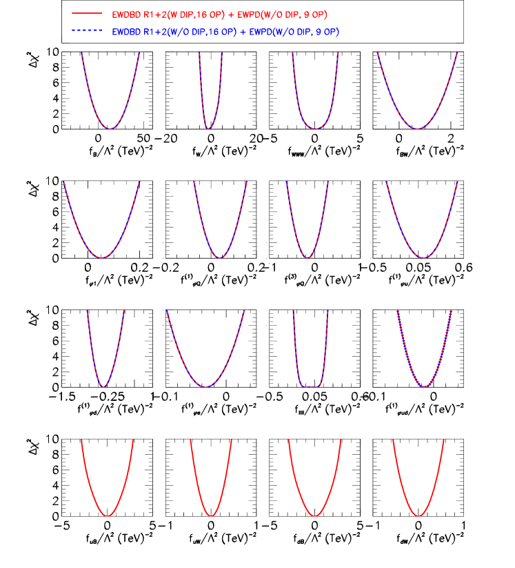
Figure 1: $\Delta\chi^{2}$ dependence on the Wilson coefficients of 16 operators (after marginalization in each panel over the undisplayed ones) entering the analysis of EWDBD from LHC Run 1 and 2 in combination with the EWPD. The red line includes the effect of light-quark dipole operators in diboson production but does not include then in the from EWPD (see Eq. 30 ). The blue dashed lines are the results of the corresponding analysis without including the light-quark dipole operators (see text for details).

III.1 Comparison with EWPD bounds

Figure 1 also illustrates the power of the high energy LHC data in diboson gauge production to impose severe constraints on the electroweak dipole couplings of the light quarks. We quantify how much these bounds improve over the ones from EWPD in Fig. 2 where we show in the red line the constraints from the above analysis together with those obtained from $Z$- and $W$-pole EWPD exclusively (black lines). To estimate the dependence of the EWPD bounds on the presence of other operators contributing to those observables we show also the results when the coefficients of all non-dipole operators are set to zero (the black dashed line in Fig. 2). As expected the bounds are only a bit stronger (about a factor O(30%)) when no other contribution is included. As mentioned above, dipole operators enter quadratically in EWDP observables so their contribution cannot cancel against that of any other dimension six-operator. The bounds derived, however, assume that there will be no cancellation against possible effects of dimension-8 operators.

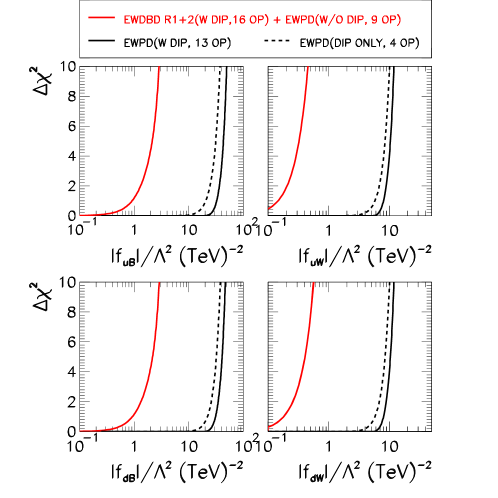
Figure 2: $\Delta\chi^{2}$ dependence on the four fermionic Wilson coefficients of the dipole operators from the combined analysis of diboson data and EWPD after marginalizing over the 15 undisplayed coefficients (full red lines), EWPD after marginalizing over the 12 undisplayed parameters (full black lines) and EWPD with only the four quark dipole operator after marginalizing over the 3 undisplayed coefficients (black dashed line).

As seen in figure 2, the bounds from EWPD are weaker than those from LHC EWDBD by more than an order of magnitude. The reason for this is two folded. First, the EWPD constraints are mainly driven by the $Z$ hadronic observables which bound the combinations $F_{qZ}/\Lambda^{2}$ in Eq. (4) which means that there is a large degeneracy between the constraints on $f_{qW}/\Lambda^{2}$ and $\tan^{2}\theta_{W}f_{qB}/\Lambda^{2}$. The degeneracy is broken only by the data on the $W$ width which is much less precisely known. Second, the contributions from dipole operators to EWDBD grow as $s$, as seen in Eqs. (22)- (27), and hence the lever arm of the high energy of LHC to constrain them.

These behaviours are explicitly displayed in Fig. 3 where we show the strong correlations in the 95% allowed region from the EWPD analysis in the plane $f_{qW}/\Lambda^{2}$ vs $f_{qB}/\Lambda^{2}$. Also shown are the corresponding rotated projection of the allowed region on $F_{qZ}/\Lambda^{2}$ vs ${F_{q}\gamma}/\Lambda^{2}$ and clearly illustrate how the EWPD bounds on the electric dipole coupling $F_{q\gamma}/\Lambda^{2}$ are visibly weaker. On the contrary, as seen in Eqs. (22)- (27), the production of pairs of electroweak gauge bosons receives independent contributions from different combinations of the effective light-quark dipole couplings to $Z$, $W$, and $\gamma$ and that help breaking the degeneracy and allow for constraining both the $Z$ and $\gamma$ dipole couplings with similar precision. This is explicitly shown in Fig. 4 where we plot the 95% allowed region from the EWDBD analysis in both planes $f_{qW}/\Lambda^{2}$ vs $f_{qB}/\Lambda^{2}$ and $F_{qZ}/\Lambda^{2}$ vs ${F_{q}\gamma}/\Lambda^{2}$.

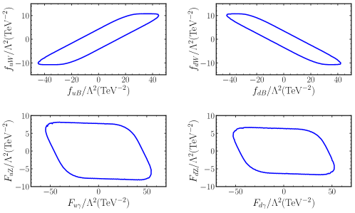
Figure 3: 95% allowed region from the EWPD analysis in planes $f_{qW}/\Lambda^{2}$ vs $f_{qB}/\Lambda^{2}$ and $F_{qZ}/\Lambda^{2}$ vs ${F_{q}\gamma}/\Lambda^{2}$.

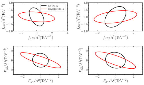
Figure 4: 95% allowed regions from the combined EWDBD analysis (red lines) and the combined DY data analysis (black lines) in the planes $f_{qW}/\Lambda^{2}$ vs $f_{qB}/\Lambda^{2}$ and $F_{qZ}/\Lambda^{2}$ vs ${F_{q}\gamma}/\Lambda^{2}$.

IV Effects in Drell-Yan Production

One of the cleanest processes at LHC is the Drell-Yan production of pairs of high invariant mass electrons and muons. Light quark dipole operators contribute to this process in the production vertex of the intermediate $Z$ and $\gamma$, and hence, can be constrained by these precise LHC results. Furthermore, the dipole operators also lead to a mild energy growth in the corresponding helicity amplitudes $q\bar{q}\rightarrow\ell^{-}\ell^{+}$ which at high energy behave as

$$A(q_{+}\bar{q}_{+}\rightarrow\ell^{-}_{-}\ell^{+}_{+})=A(q_{-}\bar{q}_{-}\rightarrow\ell^{-}_{-}\ell^{+}_{+})=\frac{e^{2}v}{\sqrt{2}}\sqrt{s}\sin\theta\left[-\frac{F_{q\gamma}}{\Lambda^{2}}+\frac{1}{c_{W}s_{W}}\left(-\frac{1}{2}+s_{W}^{2}\right)\,\frac{F_{qZ}}{\Lambda^{2}}\right]\;\;,$$ (31)

$$A(q_{+}\bar{q}_{+}\rightarrow\ell^{-}_{+}\ell^{+}_{-})=A(q_{-}\bar{q}_{-}\rightarrow\ell^{-}_{+}\ell^{+}_{-})=\frac{e^{2}v}{\sqrt{2}}\sqrt{s}\sin\theta\left[\frac{F_{q\gamma}}{\Lambda^{2}}-\frac{s_{W}}{c_{W}}\,\frac{F_{qZ}}{\Lambda^{2}}\right]\;\;,$$ (32)

where $\theta$ is the center-of-mass polar scattering angle.

Both ATLAS and CMS have published in Refs. Aad et al. (2016c) and Khachatryan et al. (2015) respectively, the final results of the Run 1 Drell-Yan measurements in the form of differential Drell-Yan cross section as a function of the invariant mass of the lepton pair after correction for detector effects and also giving a very detail account of the systematic and theoretical uncertainties after the unfolding of detector effects. This data allow us a very straightforward comparison with the invariant mass differential cross section predictions including the effect of the dipole couplings.

As for Run 2, CMS has also presented the corresponding differential cross section results but only for a small integrated luminosity Sirunyan et al. (2018a). However, both collaboration performed a search for high-mass phenomena in dilepton final states using larger Run 2 samples Aaboud et al. (2017); Sirunyan et al. (2018b). These data can also be analyzed to study the effect of dipole operators. In this case, we follow a procedure similar to that sketched in Sec. III for the analysis of EWDBD. We simulate the $e^{+}e^{-}$ and $\mu^{+}\mu^{-}$ invariant mass differential distributions within the cuts of the experimental searches using the packages MadGraph5 Alwall et al. (2014), PYTHIA6.4 Sjostrand et al. (2006) and Delphes de Favereau et al. (2014). The SM predictions from this procedure are then normalized bin by bin to the predictions provided by the experimental collaborations and the obtained correction factors are subsequently applied to the predicted distributions in presence of the dipole operators.

In summary, we include the following data samples in our Drell-Yan analysis:

	Int.Luminosity (fb-1)	$m_{\ell\ell}$	# Data points
ATLAS 13 TeV Aaboud et al. (2017)	36 fb-1	250–6000 GeV	6+6
CMS 13 TeV Sirunyan et al. (2018b)	36 fb-1	200–3000 GeV	6+6
ATLAS 8 TeV Aad et al. (2016c)	20.3 fb-1	200–1500 GeV	8
CMS 8 TeV Khachatryan et al. (2015)	19.7 fb-1	200-2000 GeV	11

and with those and the information provided by the experiments on the systematic and theoretical uncertainties and correlations we build a binned log-likelihood function

$$\chi^{2}_{\rm DY}(f_{uB},f_{uW},f_{dB},f_{dW})\;\;,$$ (33)

where for simplicity we have set to zero the coefficients of all other operators contributing to the process.

As discussed in the previous section, the amplitudes generated by dipole operators do not interfere neither with the SM ones nor with those generated by the other dimension-6 operators in Eq. (II) and, therefore, no cancellation of their effects is possible. So as it was the case in the analysis of EWDBD and of EWPD, the constraints from DY on the Wilson coefficients of dipole operators can only be marginally affected by the inclusion of other operators in the analysis.

Figure 5: $\Delta\chi^{2}$ dependence on the four fermionic Wilson coefficients of the dipole operators for the analysis of DY data (see text for details).

The results for the DY analysis are depicted in Fig. 5 where we display one-dimensional projections of the $\Delta\chi^{2}_{\rm DY}$ as a function of the Wilson coefficient of each dipole operator after marginalizing over the other three. We show the results using each of the data samples separately and the combination. As seen in the figure, the constraints imposed with the analysis of the ATLAS 8 Run 1 DY results are substantially stronger than those obtained from the analysis of the corresponding CMS Run 1 data.

We trace this difference to the fact that the ATLAS results are slightly lower than the SM predictions in all bins included in the analysis (see Table 12 in Ref. The ATLAS Collaboration ) which results in bounds which are about a twice stronger than the expected sensitivity from data centered in the SM predictions. On the contrary, CMS finds a mild excess of events with respect to the SM predictions for invariant masses between 200-500 GeV where the data is most precise (see Fig. 3 in Ref. Khachatryan et al. (2015)). This weakens their constraints by about 20%. The analysis of the Run 2 data yields bounds very much within the expected sensitivity from measurements compatible with the SM.

Comparing the results in Fig. 5 with those from EWDBD analysis in Fig. 1, we find that the combined analysis of the Drell-Yan data can yield slightly stronger (weaker) bounds on the coefficients of the quark dipole operators ${\cal O}_{qB}$ (${\cal O}_{qW}$). However, as seen in Fig. 4 DY results totally resolve the light-quark dipole couplings to $Z$ and $\gamma$ and, consequently, yield stronger constraints over those projections.

V Discussion

In this work, we have studied the power of the high energy LHC data to reveal the effects associated to electroweak dipole couplings of the light quarks. We have focused on two type of processes: pair production of electroweak gauge bosons and Drell-Yan lepton pair production. Because of their different tensor structure, the amplitudes induced by these couplings do not interfere with the SM ones nor with those generated by the other dimension-six operators that modify the gauge boson couplings to fermions and TGC’s. Consequently, we find that the constraints derived on all the Wilson coefficients of those non-dipole operators entering the tests of the electroweak gauge boson sector is robust under the inclusion of the light-quark dipole operators.

	95% CL $|f|/\Lambda^{2}$ (TeV-2)
	EWPD	EWDBD+EWPD	DY
$f_{uB}$	41	1.9	0.78
$f_{uW}$	10	0.29	0.53
$f_{dB}$	38	1.9	0.96
$f_{dW}$	10	0.36	0.60
$F_{u\gamma}$	51	1.8	0.78
$F_{uZ}$	7.0	1.3	1.2
$F_{d\gamma}$	48	1.8	0.91
$F_{dZ}$	5.8	1.4	1.4

Table 1: Comparison of the 95% upper bounds for the Wilson coefficients of the light-quark dipole operators for the different analysis performed in this work.

Dipole couplings of the light quarks to the weak gauge bosons have been explored in the past using the precise data of the on-shell $Z$ and $W$ couplings to fermions. Our results show that analyses of LHC data improves over those by more than one order of magnitude. This is explicitly quantified in Table 1 where we constrast the resulting constraints from the analysis of the data on EWDBD and DY at LHC with those from the pole measurements. The improvement is driven both by the growth of the dipole contribution with energy, and because LHC data is sensitive to the dipole couplings to $Z$ and $\gamma$’s with similar weight. Consequently, as seen in this table, the LHC bounds on the combinations entering on the dipole couplings to the $Z$ and the photon are comparable.

It is important to stress that the constraints derived with LHC data are obtained in the asymptotic free regime for the light quarks. So in this respect, the information provided by LHC complements the more model-dependent limits on the dipole couplings of the light quarks which can be derived from measurements of the anomalous magnetic moments of hadrons Brekke and Rosner (1988).