A Distributed Approach towards Discriminative Distance Metric Learning

Abstract

Distance metric learning is successful in discovering intrinsic relations in data. However, most algorithms are computationally demanding when the problem size becomes large. In this paper, we propose a discriminative metric learning algorithm, and develop a distributed scheme learning metrics on moderate-sized subsets of data, and aggregating the results into a global solution. The technique leverages the power of parallel computation. The algorithm of the aggregated distance metric learning (ADML) scales well with the data size and can be controlled by the partition. We theoretically analyse and provide bounds for the error induced by the distributed treatment. We have conducted experimental evaluation of ADML, both on specially designed tests and on practical image annotation tasks. Those tests have shown that ADML achieves the state-of-the-art performance at only a fraction of the cost incurred by most existing methods.

Index Terms – parallel computing, distance metric learning, online learning

I Introduction

Comparing objects of interest is a ubiquitous activity and defining characteristic of learning-based systems. The comparison can be explicit, as in the nearest neighbour rule, or be encoded in a learned model, as in the neural networks. In all cases, to let the past experience have any help in making decisions about unseen objects, one must compare the objects to those with known information. A natural measure is the Euclidean distance. Despite its wide application, the Euclidean distance may not suit all problems. For example, Euclidean distance is directly affected by the scaling of individual features in the representation of the data. Features of high multitude have strong influence on the measure of similarity regardless its relevance to the task. Without accounting for relevance, Euclidean distance is particularly problematic when the data is of high dimension, and the informative structures of the data population are difficult to distinguish from meaningless fluctuations.

The problem of the Euclidean distance suggests to adapt the metric in the learning process, so that distance measure is conducive to the subsequent recognition tasks. Along this line of research, a family of distance metric learning techniques has been developed [1][2][3][4][5][6][7], and proven useful in a number of practical applications [8][9]. However, a major difficulty of metric learning arises from the time and space cost of those algorithms. To construct an effective distance metric, relevance of the raw features should be evaluated w.r.t. each other, instead of individually. Given $d$ raw features, this means $d^{2}$ covariance terms to be dealt with. In cases where $d$ is large but the number of samples, $N$, is moderate, an alternative formulation of the problem allows learning metric from pair-wise correlations between samples, which entails a complexity of $N^{2}$. However, the problem becomes irreducibly complex when both $d$ and $N$ are large, which is common in practical problems. In fact, due to technical necessities such as iterations in optimisation, a realistic metric learning algorithm generally involves a complexity of the cubic order, such as $d^{3}$ or $dN^{2}$, rather than squared one, which further limits the scalability of metric learning.

The focus of this paper is to address the seemingly inexorable complexity of distance metric learning. We first develop a discriminative metric learning method, where categorical information are utilised to direct the construction of the distance metric. More importantly, the metric learning algorithm embraces the “divide-and-conquer” strategy to deal with large volume of high-dimensional data. We derive a distributed and parallel metric learning scheme, which can be implemented in consistence with the MapReduce [10] computational framework. In particular, we split a large sample into multiple smaller subsets. The basic discriminative metric learning is applied on each of the subsets. The separately learned metrics are summarised into the final result via an aggregation procedure, and the scheme is named aggregated distance metric learning (ADML), accordingly.

Corresponding to the Map steps in the MapReduce paradigm, the computation on the subsets are independent with each other, and can be conducted in parallel tasks. The data can be stored in a distributed system, and no individual subroutine needs access to the whole data at once. So the technique is less affected by the physical storage in dealing with large volume of data. The aggregation step represents the Reduce step in MapReduce, where the input of the aggregation algorithm is the learned metrics on the subsets. Aggregation takes sum of those learned metrics, where the operation collapses the inputs arriving in arbitrary order, taking only moderate space given the subspace representation of the metrics.

The whole scheme scales well with the dimension and sample size of the data. The basic discriminative metric learning algorithm adopts subspace representation of the learned metric. If the sizes of individual subsets $N_{K}$ and the subspace dimension $q$ are fixed, the space and time taken by the metric learning on the subsets grow linearly with respect to the input dimension $d$. The aggregation time grows linearly with $d$ as well. Thus in theory, the ideal implementation of ADML has desirably benign time and space cost. The time cost is linear with respect to the input dimension $d$ and independent to the total sample size $N$, and the space cost is the size of the data $d\times N$ in terms of storage and $\max(d\times q,N_{K}^{2})$ in terms of the volatile memory for on-the-fly computation, where $d\times q$ represents the size of the learned metric, and $d$ and $N$ are large compared to $q$ and $N_{K}$. For practical computational facilities, where parallel tasks are limited and incurs communication overheads, the learning and aggregation of metrics on the subsets can only be partially parallelised. Thus the time cost by ADML grows linearly with, instead of being independent to, the sample size $N$. This practically achievable time complexity still scales better with the problem size compared with wholistic methods.

We provide theoretical guarantee for the distributed computation scheme. In particular, the upper bound has been provided for deviation by which the metric obtained by ADML can differ from the one would be resulted if the discriminative metric learning were applied on the whole data. The bound of deviation supports the usage of distributed computation in metric learning, and caps the price we have to pay for the gain of efficiency.

The effectiveness of ADML has also been demonstrated by empirical study. We test the method using both synthetic data and on a practical image annotation task. The empirical results corroborate our motivation for ADML, that the distributed learning achieves much superior efficiency with little or no sacrifice of accuracy compared to state-of-the-art metric learning methods.

II Background

The need for appropriate similarity measure is rooted in the fundamental statistical learning theory, in particular in the interplay between complexity and generalisation. In general, a learning algorithm produces a predictor by matching a set of hypotheses against observed data. The theory tells that the confidence about the predictor’s performance on unseen data is affected by the complexity of the hypothesis set [11]. While the complexity of a hypothesis (function) set is gauged by the possible variations on the domain of input. Therefore, the way of measuring similarity between the data samples essentially characterises the hypothesis set and affects how a learned predictor generalises to unseen data.

It has been noticed that the intuitive measurement of Euclidean metric becomes unreliable for high dimensional data, i.e. the number of raw features is large [12]. Therefore, recently much attention has been paid to adapting the distance metrics to the data and analysis tasks. In [1], Xing et al. proposed to adaptively construct a distance measure from the data, and formulated the task as a convex optimisation problem. The technique was successfully applied to clustering tasks. An effective way of learning a metric and simultaneously discovering parsimonious representation of data is to construct a mapping, which projects the data into a subspace in which the Euclidean distance reproduces the desired metric. The link between metric learning and data representation connects the proposed method to a broad context. In [13], metric learning is formulated as a kernel learning problem, and solved via convex optimisation. Relevance component analysis (RCA) [2] learns a transformation with accounting for the equivalent constraints presenting in the data, i.e. pairs of samples are known to be of the same category and thus preferably to be measured as close to each other by the objective metric. In [3], Hoi et al. proposed discriminant component analysis (DCA), which equips RCA with extra capability of dealing with negative constraints, sample pairs to be scattered far apart by a desirable metric. Both RCA and DCA can be solved by eigenvalue decomposition, which is practically faster than the convex optimisation in [1]. When the ultimate goal of learning a distance metric is to preserve or enhance discriminative information, research has shown that the local geometry in the neighbourhoods of individual samples is effective. The raw features can be assessed by [14, 15] by their contribution to the posterior probabilities at individual samples. In [4], a learning scheme has been proposed to optimise classification based on nearest neighbour rule. Large margin objective has also been proven effective in deriving supervised metric learning approaches [5, 7]. In [6], a scheme has been developed to incorporate auxiliary knowledge to assist metric learning. More comprehensive overview of related research can be found in [12]. As we have discussed in the last section, a major concern of most existing metric learning approaches is the scalability. For example, the constrained convex programming [1, 2, 3, 4, 5] limits their applicability in large-scale practical problems.

Online processing is another strategy of solving large scale problem [16], which is complement to parallel computing and often of practical interest when dealing with data from the web. Online distance metric learning algorithms has been proposed [17][18]. These online metric learning techniques are based on serial steps, where the metric is updated after new observations arrive. Serial online schemes are able to deal with large problems, but slow to arrive the final solution. To improve efficiency, parallel implementation is a natural strategy. Many basic operations have fast parallelised implementation, such as Intel’s Math Kernel Library; and some learning techniques are parallelised at the algorithm level [19][20][21]. While ADML is a novel metric learning method supporting fully distributed realisation, where subset metrics can be computed on different subsets simultaneously, and with reduced computational cost.

III Discriminative distance metric learning

We are concerned with constructing a Mahalanobis distance metric in the data feature space, which incorporates the discriminative information, i.e. the class membership of individual samples. In particular, the Mahalanobis distance between $\mathbf{x}_{i},\mathbf{x}_{j}\in\mathbb{R}^{d}$ is defined by a positive semi-definite matrix $\mathbf{Q}\in\mathbb{R}^{d\times d}$, $d_{\mathbf{Q}}^{2}(\mathbf{x}_{i},\mathbf{x}_{j})=(\mathbf{x}_{i}-\mathbf{x}_{j})^{T}\mathbf{Q}(\mathbf{x}_{i}-\mathbf{x}_{j}).$ The goal of the proposed discriminative distance metric learning (DDML) is to find a matrix $\mathbf{Q}$, so that $d_{\mathbf{Q}}$ between samples of the same class tends to be small and that between samples of different classes tends to be large. Such a distance metric will benefit subsequent tasks such as classification or recognition.

However, a universally satisfactory Mahalanobis distance metric $\mathbf{Q}$ is usually difficult to obtain. Practical data are often complex objects consisting of many features, where the number of features, $d$, is much greater than the actual degrees of freedom. Thus the variations in the data span nonlinear low-dimensional manifolds precluding global Mahalanobis distance metric. To preserve the nonlinear structures in the data, we set up the learning objective locally and let a local metric encodes both the discriminative information and the local geometric structure of the data. The overall distance metric is computed by unifying all the local metrics in an optimisation framework.

In particular, the cost of a distance metric is defined on data patches associated with individual samples. Given a sample $\mathbf{x}_{i}$, the corresponding patch consists of a small number of samples that are close to $\mathbf{x}_{i}$ and carrying discriminative information. In particular, we select the $k_{W}$ nearest neighbours $\mathbf{x}_{N_{i}^{W}}$ from the same class as $\mathbf{x}_{i}$, and select $k_{B}$ nearest neighbours $\mathbf{x}_{N_{i}^{B}}$ from different classes. The patch, $\mathbf{X}_{N_{i}}$, is the joint of $\{\mathbf{x}_{i}\}\cup\mathbf{x}_{N_{i}^{W}}\cup\mathbf{x}_{N_{i}^{B}}$.

The local criterion of metric learning on $\mathbf{X}_{N_{i}}$ is motivated by encoding the discriminative information into the geometry induced by the objective metric. A local metric $\mathbf{Q}_{i}$ specifies the within- and between-class distances on $\mathbf{X}_{N_{i}}$ as

$$D^{\{W,B\}}(\mathbf{X}_{N_{i}},\mathbf{Q}_{i})= \sum_{j\in N_{i}^{\{W,B\}}}d_{\mathbf{Q}_{i}}^{2}(\mathbf{x}_{i},\mathbf{x}_{j})$$ (1)

Furthermore, to account for the locally linear geometry of the data manifold, $\mathbf{Q}_{i}$ is considered as being induced by a subspace projection $\mathbf{W}_{i}$, where $d_{\mathbf{Q}_{i}}^{2}(\mathbf{x}_{i},\mathbf{x}_{j})=\|\mathbf{W}_{i}^{T}(\mathbf{x}_{i}-\mathbf{x}_{j})\|^{2}$. Note that such a subspace representation of the Mahalanobis distance implies a concise parameterisation of $\mathbf{Q}_{i}=\mathbf{W}_{i}\mathbf{W_{i}}^{T}$.

Therefore, the principle of metric learning becomes an optimisation over local transformation $\mathbf{W}_{i}$,

$$\mathbf{W}_{i} =\arg\min_{\mathbf{W}}\big{\{}{\textstyle\sum_{j\in N_{i}^{W}}}\|\mathbf{W}^{T}(\mathbf{x}_{i}-\mathbf{x}_{j})\|^{2}$$ (2)

$$\qquad\ \ \ -\beta{\textstyle\sum_{j\in N_{i}^{B}}}\|\mathbf{W}^{T}(\mathbf{x}_{i}-\mathbf{x}_{j})\|^{2}\big{\}}$$

$$=\arg\min_{\mathbf{W}}\textrm{tr}\left(\mathbf{W}^{T}\mathbf{X}_{N_{i}}\mathbf{L}_{i}\mathbf{X}_{N_{i}}^{T}\mathbf{W}\right)$$

where $\beta$ is a trading-off between small $D^{W}$ and large $D^{B}$; and $\mathbf{L}_{i}$ is obtained by organising the coefficients of the quadratic form,

$$\mathbf{L}_{i}= {\textstyle\left[\begin{array}[]{cc}{\displaystyle{\textstyle\sum_{j}}\left[\mathbf{\omega}_{i}\right]_{j}}&-\mathbf{\omega}_{i}^{T}\\ -\mathbf{\omega}_{i}&\mathrm{diag}(\mathbf{\omega}_{i})\end{array}\right]}$$

where $\omega_{i}$ is a row vector concatenated by $N_{i}^{W}$ $[1]$’s and $N_{i}^{B}$ $[-\beta]$’s, and $\mathrm{diag}(\cdot)$ represents an operator generating an $n\times n$ diagonal matrix from an $n$-dimensional vector.

Unifying the optimisations on individual local patches, we reach the objective function for global distance metric learning,

$$\mathbf{W}_{G} =\arg\min_{\mathbf{W}}\sum_{i}\textrm{tr}\left(\mathbf{W}^{T}\mathbf{X}_{N_{i}}\mathbf{L}_{i}\mathbf{X}_{N_{i}}^{T}\mathbf{W}\right)$$

$$=\arg\min_{\mathbf{W}}\,\textrm{tr}\left(\mathbf{W}^{T}\mathbf{X}\mathbf{L}\mathbf{X}^{T}\mathbf{W}\right),$$ (4)

where $\mathbf{L}=\sum_{i}\mathbf{S}_{i}\mathbf{L}_{i}\mathbf{S}_{i}^{T}$ and $\mathbf{S}_{i}$ is an $|\mathbf{X}_{N_{i}}|\times N$ matrix selecting the samples in a local patch from the data set, so that $\mathbf{X}_{N_{i}}=\mathbf{X}\mathbf{S}_{i}$.

The DDML objective (4) is readily solved by eigenvalue decomposition, where the columns of $\mathbf{W}$ are of the vectors associated with the smallest eigenvalues of $\mathbf{X}\mathbf{L}\mathbf{X}^{T}$. Generally, the eigenvalue decomposition involved in solving $\mathbf{W}$ in (4) will be more efficient than methods based on iterative convex optimisation methods, e.g. NCA [2] and LMNN [5].

For most practical applications, DDML is still facing several difficulties, because both the volume and dimension of practical data are usually high, and also because in real-life applications, the data is often organised in distributed databases and acquired as streams. In the following section, we will address these problems by applying the idea of “divide and conquer” [22] to DDML and propose a scalable aggregated distance metric learning algorithm.

IV Aggregated Distance Metric Learning

In this section, we first introduce the distributed computation of DDML, aggregated distance metric learning (ADML), and then prove that metric learned by ADML is consistent with the result of performing DDML directly on the entire dataset. We further improve the efficiency of ADML by introducing an alternative aggregation technique, and show its consistency attributes. The time and spatial complexities are discussed for the proposed algorithms with an important observation that we can compute discriminative metric learning independent of the data size and only linearly depending on the data dimension.

IV-A Aggregated Distance Metric Learning

The idea of ADML can be sketched as follows: dividing the whole data into several subsets, performing DDML on each of the subset and finally aggregating the results into a consolidate solution. It is important not to confuse the split of data in ADML with the use of local patch in DDML. We recall that the objective function in DDML is defined on a patch-by-patch base to account for the local geometry of the data manifold, where each patch is constructed with regard to the entire dataset. While in ADML, subsets are generally not associated with local geometry (preferably so), and only one of the subsets is visible to a DDML algorithm.

We randomly split a dataset $\mathbf{X}$ of $N$ samples into $K$ subsets $\mathbf{X}_{k=1,\dots,K}$. This reduces the cost of constructing patches in metric learning: in ADML, the patch of a sample is constructed by finding nearest neighbours within the subset to which the sample is belonging.

Let the objective function of learning $\mathbf{W}$ in (4) be $F(\mathbf{W})$. Using the similar form as $F$, we can derive a local objective function with respect to a subset $\mathbf{X}_{k}$,

$$F_{k}(\mathbf{W}) =\textrm{tr}\left(\mathbf{W}^{T}\mathbf{R}_{k}\mathbf{W}\right),$$ (5)

where $\mathbf{R}_{k}=\mathbf{X}_{k}\mathbf{L}_{k}\mathbf{X}_{k}^{T}$ and $\mathbf{L}_{k}$ is defined similarly to $\mathbf{L}$ in (4), but is confined within $\mathbf{X}_{k}$. The metric on subset $k$ is then characterised by $F_{k}$, where we denote the local solution be $\mathbf{W}_{k}$.

The next task is to consolidate the local solutions $\{\mathbf{W}_{k}\}$ into a global metric $\mathbf{W}_{A}$. Straightforward linear combination would be the most intuitive approach. However, $\{\mathbf{W}_{k}\}$ are solutions to locally defined optimisation problems and linear interpolation may damage their optimality and yield invalid solutions. Therefore, we design the aggregation based on the optimal conditions of the objective functions. A local solution $\mathbf{W}_{k}$ is a stationary point of the corresponding $F_{k}$, where the gradient vanishes,

$$\frac{\partial F_{k}(\mathbf{W}_{k})}{\partial\mathbf{W}_{k}}=2\mathbf{R}_{k}\mathbf{W}_{k}=0,\ \textrm{for}\ k=1,\dots,K.$$ (6)

Recall that $\mathbf{R}_{k}$ is defined in (5). For a global solution $\mathbf{W}_{G}$, it is ideal for it to fulfil condition (6) in all local subsets $k=1,\dots,K$, which is generally impossible. Thus secondarily, we want the violations to cancel out among all the $K$ subsets and the sum of local gradients to vanish

$$\sum\limits_{k=1}^{K}\mathbf{R}_{k}\mathbf{W}_{A}=0.$$ (7)

Directly summing up (6) over $k$, we reach

$$\sum\limits_{k=1}^{K}\mathbf{R}_{k}\mathbf{W}_{k}=0.$$ (8)

Comparing (8) and (7) gives an aggregation rule: the overall solution $\mathbf{W}_{A}$ satisfies

$$0 =\sum_{k=1}^{K}\mathbf{R}_{k}\mathbf{W}_{k}-\sum_{k=1}^{K}\mathbf{R}_{k}\mathbf{W}_{A}$$ (9)

$$\textrm{thus }\mathbf{W}_{A} =\left(\sum_{k=1}^{K}\mathbf{R}_{k}\right)^{-1}\left(\sum_{k=1}^{K}\mathbf{R}_{k}\mathbf{W}_{k}\right).$$ (10)

The computation of (10) is intuitively plausible: the aggregation has the form of interpolation of the local $\mathbf{W}_{k}$ with the “weights” being $\mathbf{R}_{k}$. We will show that the aggregation also enjoys desirable theoretical attributes in following discussions.

There are two further remarks regarding the derivation and computation of the aggregation. First, directly solving for $\mathbf{W}_{k}$ following (5) involves eigenvalue decomposition of a $d\times d$ matrix, which is expensive when $d$ is large. The cost can be alleviated by exploiting that $\mathbf{R}_{k}$ is known to be decomposed as $\mathbf{X}_{k}\mathbf{L}_{k}\mathbf{X}_{k}^{T}$. In the scenario of a large $d$, a subset $\mathbf{X}_{k}$ generally has $|\mathbf{X}_{k}|<d$ and samples independent vectors in $\mathbb{R}^{d}$. Thus $\mathbf{W}_{k}$ can be represented as $\mathbf{X}_{k}\mathbf{U}_{k}$. Solving for $\mathbf{W}_{k}$ becomes finding $\mathbf{U}_{k}$ such that

$$\mathbf{X}_{k}\mathbf{L}_{k}\mathbf{X}_{k}^{T}\mathbf{X}_{k}\mathbf{U}_{k} =\mathbf{X}_{k}\mathbf{U}_{k}\mathbf{\Lambda}_{k},$$

where $\mathbf{\Lambda}_{k}$ is a diagonal matrix. It is sufficient to find a $\mathbf{U}_{k}$ where $\mathbf{L}_{k}\mathbf{X}_{k}^{T}\mathbf{X}_{k}\mathbf{U}_{k}=\mathbf{U}_{k}\mathbf{\Lambda}_{k}$, where translates to an eigenvalue decomposition of an $|\mathbf{X}_{k}|\times|\mathbf{X}_{k}|$ matrix $\mathbf{L}_{k}\mathbf{X}_{k}^{T}\mathbf{X}_{k}$.

The second remark is on the relation between the two characteristics $\mathbf{W}$, the solution of local DDML: (i) $\mathbf{W}$ is obtained by eigenvalue decomposition and minimises (5) and (4) and (ii) $\mathbf{W}$ satisfies stationary point condition (6). We do not include the orthogonal constraint on $\mathbf{W}$ in (6), because at the aggregation stage, we have already got the local solutions complying with the constraint. In fact, if we consider one column of $\mathbf{W}$ and formulate the orthogonal constraint using Lagrange multiplier, $L=\mathbf{w}^{T}\mathbf{R}\mathbf{w}-(\lambda\mathbf{w}^{T}\mathbf{w}-1)$, then the stationary condition with respect to $L$ leads to the solution of eigenvalue decomposition.

IV-B Consistency of Aggregation

In this section, we prove that the aggregated distance metric is consistent with the one we would achieve if we performed the learning using a wholistic approach. The essential idea in brief is as follows.

The law of large numbers dictates that the empirical solution of (4), say, $\mathbf{W}_{G}$, approaches to an “ideal solution” $\mathbf{W}_{0}$, the solution to (4) if we could have constructed the problem using the entire data population as $\mathbf{X}$. We first notice that the same argument applies to the local solutions $\{\mathbf{W}_{k}\}$ – solution of (4) on a subset $\mathbf{X}_{k}$ approaches $\mathbf{W}_{0}$ as $\mathbf{X}_{k}$ start including infinitely many random samples, which is the case because of the random split of data. Thus to show the aggregated solution $\mathbf{W}_{A}$ approaches the wholistic solution $\mathbf{W}_{G}$, we can show that both of them approach $\mathbf{W}_{0}$. We prove $\mathbf{W}_{A}$ approaches $\mathbf{W}_{0}$ through $\{\mathbf{W}_{k}\}$. In fact, our key contribution is to establish that given some target $\hat{\mathbf{W}}$, the distance between the aggregated solution $\mathbf{W}_{A}$ and $\hat{\mathbf{W}}$ is bounded in terms of the distance between the local solutions $\mathbf{W}_{k}$ and $\hat{\mathbf{W}}$ (by a constant factor). The result is formally specified by the following theorem.

Theorem 1.

Let $\{\mathbf{W}_{k}\}$ be the local solutions to (5) on the subsets. If $\mathbf{R}=\sum_{k}\mathbf{R}_{k}$ in (10) is invertible and $\mathbf{W}_{G}$ is the aggregation of $\{\mathbf{W}_{k}\}$, we have $\|\mathbf{W}_{A}-\hat{\mathbf{W}}\|\leq S_{1}\sup_{k}\{\|\mathbf{W}_{k}-\hat{\mathbf{W}}\|\}$ for some target $\hat{\mathbf{W}}$, where

• $\|\cdot\|$ represents the spectral norm of a matrix, $\|\mathbf{A}\|=\sqrt{\lambda_{max}(\mathbf{A}^{T}\mathbf{A})}$, where $\lambda_{max/min}$ stands for the maximum or minimum eigenvalue of a matrix;

• $S_{1}=\frac{K\max_{k}\{\lambda_{max}(\mathbf{R}_{k})\}}{\lambda_{min}(\mathbf{R})}$, and $K$ is the number of subsets.

Moreover, if each $\mathbf{R}_{k}$ is positive definite, we have $\|\mathbf{W}_{A}-\hat{\mathbf{W}}\|\leq S_{2}\max_{k}\{\|\mathbf{W}_{k}-\hat{\mathbf{W}}\|\}$, where $S_{2}=\frac{\max_{k}\{\lambda_{max}(\mathbf{R}_{k})\}}{\min_{k}\{\lambda_{min}(\mathbf{R}_{k})\}}$.

We sketch the proof of the theorem as follows, and provide technical details in Appendix. The first part, i.e. $\|\mathbf{W}_{A}-\hat{\mathbf{W}}\|\leq S_{1}\max_{k}\{\|\mathbf{W}_{k}-\hat{\mathbf{W}}\|\}$, is achieved by applying matrix triangle inequality [23] and then manipulating the max/min eigenvalues for each item in the summation. For the second part, the proof is similar to the first part, additionally, with a bound of $\lambda_{min}$ of $\mathbf{R}$ being derived in terms of $\lambda_{min}$ of individual $\mathbf{R}_{k}$.

By replacing the target matrix $\hat{\mathbf{W}}$ with $\mathbf{W}_{0}$ and $\mathbf{W}_{G}$, Theorem 1 straightforwardly shows the consistency of ADML.

IV-C Orthogonalised Aggregated DML

We have introduced ADML algorithm and shown that its divide-and-conquer scheme is valid in theory. However, for practical implementation, inverting $\mathbf{R}=\sum_{k}\mathbf{R}_{k}$ for aggregation is a computationally demanding step if the dimension of data is high. In this section, we will introduce an efficient operation to replace the matrix inversion, as well as show that the alternate implementation of aggregation enjoys consistency attributes similar to what we have established above.

We recall our earlier discussion that $\left(\sum_{k}\mathbf{R}_{k}\right)^{-1}$ in (10) serves as a normalising factor in a matrix interpolation. To avoid computing the inversion, we employ singular value decomposition (SVD) for the mixing of the mapping matrices in the weighted sum $\sum_{k}\mathbf{R}_{k}\mathbf{W}_{k}$. SVD is relatively inexpensive compared to inversion, because in general we let $\mathbf{W}$ be a mapping to a subspace of much lower dimension than the raw data space, and $\mathbf{W}$ has much less columns than rows. Formally, we define the new aggregation rule by the following SVD

$$\mathbf{W}_{A}\mathbf{D}\mathbf{V}^{T} =\sum_{k=1}^{K}\mathbf{R}_{k}\mathbf{W}_{k},$$ (11)

where $\mathbf{D}$ is a diagonal matrix and $\mathbf{V}$ has orthonormal columns. We summarise the steps for a practical implementation of ADML in Algorithm 1. The consistency attributes are established by the following theorem.

Theorem 2.

Given locally learned $\mathbf{W}_{k=1,\dots,K}$ and aggregated $\mathbf{W}_{A}$ by rule in (11), we have $\|\mathbf{W}_{A}-\hat{\mathbf{W}}\|\leq KS_{3}\max_{k}\left\{\left\|\mathbf{W}_{k}-\hat{\mathbf{W}}\right\|\right\}+S_{3}+1$ for some target $\hat{\mathbf{W}}$, where $S_{3}=\lambda_{max}(\mathbf{R})/\min\{\mathrm{diag}(\mathbf{D})\}$.

A proof of Theorem 2 can be reached following the similar route of proving Theorem 1. The details are provided in Appendix. The consistency of the alternated aggregation can then be established.

IV-D Temporal and Spatial Complexity

Table I: Step-wise Time Complexity

ADML-I represents the aggregation by the rule of (10); and ADML-II represents aggregation by rule (11). $M=\min\{N,d\},\ M_{K}=\min\{N_{K},d\}$, $N$: total number of samples, $N_{K}$: number of samples in individual subsets $d$: data dimension, $K$: number of subsets, $q$: number of columns in $\mathbf{W}$.

One of the main motivations of ADML is to scale metric learning up for practical applications. Table I lists the time complexity of the steps of the learning algorithms discussed in this section. Note that the complexity of ADML algorithms are for serial processing of $K$ subsets, each of size $N_{K}$. However, ADML can be parallelised. Independent sub-routines of subset metric learning can be carried out simultaneously. The time of the metric learning on subsets can be accelerated by a factor up to $K$. The spatial complexity of the aggregated algorithms is also smaller than that of the straightforward implementation of DDML. In a parallel implementation, each computational node needs only to store one subset in its memory, and the computation takes less memory as well.

V Experiments

In this section, we conduct experimental studies on synthetic and real data to validate the proposed metric learning technique. In all the tests, the aggregation rule discussed in Sec. IV-C is employed (ADML-II, referred to as ADML hereafter), because it has superior temporal and spatial efficiency. We assess the methods by how the learned metric aids data representation, as well as their empirical costs of computational resources.

V-A Experiments on synthetic data

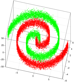
Figure 1: A set of data points drawn from the synthetic distribution. The green and red points belong to two classes, being slightly disturbed from two coiled surfaces. Note the range of the data distribution along the Z-axis (the one that is mostly perpendicular to the canvas) is greater than those along the X-Y axis.

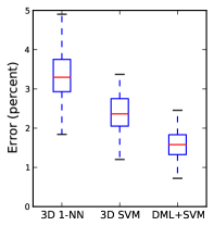
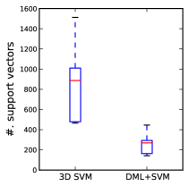
(a)                                         (b)

Figure 2: How distance metric learning and subspace mapping affect classification. (a) comparison between three classification tests: nearest neighbour rule and SVM in the raw 3D data space, and SVM in projected 2D space. (b) number of support vectors the SVMs used in 3D and 2D spaces.

The algorithm is first tested on synthetic data consisting of two classes of 3D points distributed on two curved surfaces. The surfaces are coiled together in the 3D space, and the data points deviate away from the surfaces by small disturbances. The experiment has been repeated 20 times using randomly sampled datasets, each containing approximately 17,000 samples. Fig. 1 illustrates one set of samples drawn from the population. In this experiment, we will first verify the principal motivation that an appropriate distance metric helps analysis, before turning to the distributed implementation of ADML.

The first test is by using the basic method developed in Sec. III, which allows us to examine the effect of DML without complication caused by any divide-aggregation scheme. The metric is represented by a $3\times 2$ matrix $\mathbf{W}$, because the variance relevant to classification spans across two dimensions (the X- and Y-axis). Although DML naturally lends itself to classification by nearest neighbour rule, which will be our classifier of choice in the following experiments, for the basic idea verification, we will use an SVM as the classifier. This is to confirm that DML and the subsequent subspace mapping represent the data in a form that benefits generic analysis. The basic DML algorithm has been applied to a subset of about 3,500 samples of each of the 20 random datasets, where the sample size is reduced due to the high computational cost of the straightforward optimisation of (4). Of each subset, 80% samples are used for training and validation and 20% for testing. Validation on the first subset shows that DML is insensitive to the algorithm parameters, so the chosen parameter set $k_{W}=10$, $k_{B}=20$ and $\beta=0.1$ is used throughout this experiment (including following experiments of ADML on the full datasets). Note that DML without model selection in most (19 out of 20) tests has a subtle beneficial effect on the generality of the results: our primary goal is to examine whether DML helps analysis for a generic scenario; and thus the choice of SVM as the classifier in the test stage should remain unknown to the DML algorithm in the training stage as the data transformer, in order to prevent the DML being “overfit” to SVM-oriented metrics. The parameters of SVM have been determined by cross-validation in all tests. Fig. 2 (a) shows the classification performance by the first nearest neighbour rule, SVM in the 3D data space and SVM in the DML-mapped 2D space. From the figure, one can tell a meaningful improvement of classification performance achieved by providing SVM the DML-mapped data over that of applying SVM on the raw data. The results clearly show the DML-induced subspace mapping does not only preserve useful information, but also make the information more salient by suppressing irrelevant variance through dimension reduction. Furthermore, in the DML-mapped space, the superior classification performance has been achieved at a lower computational cost. Fig. 2 (b) displays the statistics of the number of support vectors used by the SVMs in the raw 3D space and the DML-mapped 2D space. In the reduced space, SVM can do with a fraction of the support vectors that it has to use in the raw data space for the same job.

In the second part of this experiment, we will examine our main idea of the divide-aggregate implementation of DML, i.e. the ADML algorithm. For the remaining tests in this subsection, each full dataset is split into 50-50% training and test subsets. The main focus is how the division of the training data affects the learned distance metrics.

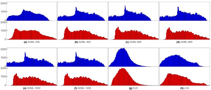
Figure 3: Statistics of pair-wise distances of within- and between-class point pairs. Each subplot contains two histograms. The upper (blue) histogram shows distances between 10,000 same-class point pairs, normalised into [0,1]. Similarly, the lower (red) histogram corresponds to cross-class pairs. Subplots (a–f) display distance measured by ADML with different subdivisions of the data (subset size ranging from 200 to 1,200). Subplot (g) displays the histograms of Euclidean distance (EUC) and (h) shows histograms of LDA-induced distance (LDA).

Fig. 3 shows a close and explicit inspection of how the learned distance metrics are connected to the class membership of the data. We randomly sample 10,000 pairs of points, compute the distance between the pair according to the learned metrics and normalise the distances to $[0,1]$. Then two histograms are generated from the set of normalised distance, one for those that both points in the pair are from the same class, and another histogram corresponds to those that the pair of points are from different classes. The two histograms are shown in the subplots in Fig. 3, where the upper (blue) part represents the same-class pairs and the lower (red) part represents the cross-class pairs. A good metric should make the cross-class distance greater than the same-class distance, especially for those smallest distances, which correspond to nearest neighbours. The subplots in the figure compare such statistical distinctions of several metrics. As shown by the figure, DML leads to more informative distance metric than the original Euclidean metric in the 3D space, which is consistent with what we have observed in the earlier part of this experiment. For comparison, the widely used linear discriminative analysis (LDA) has also been used to project the data to 2D. Fig. 3 shows that LDA-induced distance metric make distinctions between the same- and cross-class point pairs, but the difference is less than that resulted by ADML-learned metric. A possible explanation is that the same-class covariance of these datasets is close to the cross-class covariance. Thus LDA, relying on the two covariance statistics, suffers from the confusion between the two groups of covariance.

More importantly, the results shows ADML is reasonably stable over the aggressive sub-divisions of the data. In particular, because ADML trades accuracy for speed, ideally the sacrifice of performance would be mild with regard to the partition of the data into smaller subsets (lower costs). The results show that in these tests, the resultant distance metric begins to help classification when the subset size is as small as 200, and becomes distinctive between same- and cross-class pairs when the subset size is greater than 400. Therefore the parallel computation approximates the discrimination objective satisfactorily.

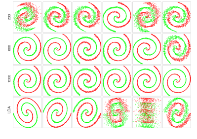
Figure 4: 2D projections induced by metric learning. The figure shows 2D projections obtained by ADML (first three rows of different subset sizes, 200, 600 and 1200) and LDA (last row) to project six randomly generated datasets (columns). Projections distinguishing samples from the two classes (green and red, better viewed in colours on screen) are more preferred.

If a learned metric is represented by $\mathbf{W}$ and the data points are $\mathbf{X}$, $\mathbf{W}^{T}\mathbf{X}$ represents a low dimensional projection. The data points in the projection space reflect the geometry induced by the learned metric. Fig. 4 shows the projections of six random datasets, where the projections are produced by ADML using different data partitions, as well as by LDA. It is interesting to see that given only 200 samples to individual local learners, ADML starts producing projections that distinguish the two classes. With larger sample sizes, the results are more reliable and the projections become more discriminative. On the other hand, with all samples for training, LDA performed unstably in these datasets, which may be due to the large irrelevant component in the data covariance, as we have discussed above.

V-B Automatic Image Annotation

For a practical test, we apply metric learning algorithms to find helpful distance measure for automatic annotation. Given a list of interested concepts, the task of annotating an image is to determine whether each of the concepts is present in the image. Essentially, annotation is to establish a connection between the content of an image and its appearance, which is known as the problem of semantic gap [24]. A natural solution to the problem is to identify the image in question with respect to a set of reference images that have been labelled with interested tags of concepts. Therefore, given the features of visual appearance, successful annotation relies on finding useful geometry in the appearance space, which reflects the connection between images in the semantic space; and annotation will benefit from effective metric learning methods. In the following report, we discuss the details of applying metrics learned by different techniques to annotate a large scale image dataset.

V-B1 Task specification and evaluation criterion

The NUS-WIDE dataset [25] has been used for the annotation test. The dataset has been compiled by gathering publicly available images from Flickr. To facilitate comparison, the visual appearance of each image is represented by six sets of standard features. These features are: colour histogram (of 64 bins), colour correlogram (of 144 bins), edge direction histogram (of 73 bins), wavelet texture (of 128 coefficients), block-wise colour moments (of 255 elements), and bag-of-words feature based on the SIFT descriptors (of 500 bags). There are totally 1134 visual features for each image. The raw data are centred at zero, and each feature is normalised to have unit variance. The task is to choose from 81 tags for each image. The tags are determined independently, thus each image can have more than one tag.

The annotation procedure is based on the nearest neighbour rule. To decide the contents of an image, up to 15 of its nearest neighbours are retrieved according to the tested distance metric. We compare the level of presence of the tags among the nearest neighbours of an image with their background levels in the reference dataset, and predict the tags of the test image accordingly. If a tag is assigned to $r_{0}$ percent of all images in the reference dataset, and is assigned to $r_{1}$ percent of images among the nearest neighbours, the tag is predicted to be present in the test image if $r_{1}>r_{0}$. The number of nearest neighbours used for predicting the tags has been determined by cross validation in our tests (from 1 to 15). The nearest neighbour rule has been shown effective for the annotation task [26]. More importantly, compared to other (multi-label) classification methods, the nearest neighbour rule provides the most direct assessment of the learned distance metrics using different techniques. The annotation reflects how the semantic information in the reference set is preserved in the learned distance metric in the appearance feature space.

F1-scores is measured for the prediction performance of each tag among the test images. The average value of all the tags is reported as a quantitative criterion. Having predicted the tags for a set of test images, the F1-score is measured as suggested in [27], with the following combination of precision and recall

$$F1 =\frac{2\times\textrm{precision}\times\textrm{recall}}{\textrm{precision}+\textrm{recall}}$$ (12)

where precision and recall are two ratios, “correct positive prediction to all positive prediction” and “correct positive prediction to all positive”. F1 score ranges from 0 to 1, higher scores mean better result.

In the experiment, ADML and state-of-the-art distance metric learning methods are tested, as well as several baseline metrics particularly designed for image annotation. These distance metrics are:

• Baseline, Euclidean (Base-EUC): the basic baseline metric is the Euclidean distance in the space of raw features (normalised to zero-mean and unit-variance). This metric does not require training.

• Baseline, Joint Equal Contribution (Base-JEC): suggested by [28], this baseline attributes equal weights to the six different types of image features. This metric does not require training.

• Baseline, $L_{1}$-penalised Logistic Regression (Base-LR): also suggested by [28], this baseline attributes $L_{1}$-penalised weights to the six types of image features to maximise dissimilarity and minimise similarity according to given tags. This metric is requires adaptation of the weights. However, after preprocessing, the penalised regression problem is basic and without altering the Euclidean metric of individual feature set. Thus we do not consider the training cost.

• Tag Propagation (TagProp): suggested by [29], a specialised image annotation method. This technique weighs the six feature sets by considering the nearest neighbours of individual images.

• Distance metric learning methods discussed in Section II including Xing et al.’s method (Xing) [1], Relevance Component Analysis (RCA) [2], Discriminative Component Analysis (DCA) [3], Large Margin Nearest Neighbour Classifier (LMNN) [5] and Information-Theoretic Metric Learning (ITML) [17].

For Xing, RCA, DCA, ITML and ADML, the supervision is in the form of similar/dissimilar constraints. In the tests, 100,000 image pairs are randomly sampled from the dataset to measure the “background” number of shared concepts between images. Then a pair of image is considered similar if they share more concepts (common tags) than the background number, or dissimilar otherwise.

In all the tests, algorithm parameters are chosen by cross validation. For ADML, the important settings are as follows. The number of columns of matrix $\mathbf{W}$ varies from $50$ to $100$ (subspace dimension). The within-class neighbourhood size $k_{1}$ varies from $1$ to $20$ and the between-class neighbourhood size $k_{2}$ varies from $20$ to $80$. The coefficient $\beta$ has been chosen from $0.1$ to $2.0$. We have tried different sizes for the subsets from $200$ to $1,000$.

V-B2 Test on medium-sized subsets

We first access the learned and baseline metrics with respect to different sizes of data and different levels of complexity of the annotation task. Four medium-sized subsets of the NUSWIDE datasets are compiled. Each subset consists of images with a small number (2-5) of labels. In particular, we take the two most popular concepts in the dataset, then let Subset I contain images with tags of at least one of the two concepts. Subset II subsumes Subset I, and includes extra images of the third most popular concepts. The construction carries on until we have Subset IV consisting of images with the five most popular concepts. Of all the samples in each subset, 60% of the samples are used for training and 40% for test. Among the training samples, about 15% are withheld for cross validation to fix algorithm parameters.

Table II: Annotation Performances and Time Costs on Subsets I-IV of the NUS-WIDE Dataset.

Each column represents a measure of distance. Each subset corresponds to a pair of rows, where “trn/tst” represents the number of training (including validation) and test samples, "F1": the average F1-scores of predicting the labels as defined in (12), "T": the wall time of the training stage. Detailed explanation of the results and further analysis are provided in Subsection V-B2.

The annotation and evaluation processes follow the discussion above. The average F1-scores achieved by each metric in each subset are listed in Table II. The results show that accuracy of predicting the concepts is affected by the distance metrics. When the task becomes more complex (to predict more concepts), the learned metrics are increasingly more helpful than the baseline metrics derived from the standard Euclidean distance. More specifically, in these tests, the more effective learning techniques are those considering the local discriminative geometry of individual samples, such as ITML, LMNN and ADML, compared to those working on the global data distribution, such as DCA and RCA. In all the tests, ADML has provided a distance metric achieving superior or close-to-the-best annotation performance.

More relevant to our main motivation of the efficiency of metric learning, Table II lists the time cost of the tested techniques. We report the wall time elapsed during the training stage of the algorithms. In addition to theoretical computational complexity, wall time also provides a practical guide of the time cost. This is important because the parallel processing of ADML needs a comprehensive assessment including the communication time and other technical overheads, which is difficult to gauge using only the CPU time of the core computations. The discussion in [30] provides a more comprehensive view of complexity in the light of parallel computation.

The reported time has been recorded on a computer with the following configuration. The hardware settings are 2.9GHz Intel Xeon E5-2690 (8 Cores), with 20MB L3 Cache 8GT/s QPI (Max Turbo Freq. 3.8GHz, Min 3.3GHz) and 32GB 1600MHz ECC DDR3-RAM (Quad Channel). We have used the Matlab implementation of the metric learning algorithms (Xing, RCA, DCA, ITML and LMNN) provided by their authors. To facilitate comparison, we implement ADML in Matlab as well, with the help of Parallel Computation Toolbox. The algorithms are run on Matlab 2012b with six workers.

In the tests, ADML has achieved good performance with high efficiency. Moreover, at the algorithmic level, the relative advantage of ADML could be greater than that is shown by the practical results in Table II. First, all algorithms are tested on the same Matlab environment, which in the background invokes Intel Math Kernel Library (MKL) for the fundamental mathematical libraries. MKL accelerates all algorithms, however, MKL competes with ADML’s parallel local metric learners for limited cores on a machine. It can be expected that ADML will benefit greater from increasing number of processors than the rival algorithms. This will also apply if advanced computational hardware is utilised such as GPU- or FPGA-based implementations[31, 20]. Second, multiple subset sizes (from 200 to 1,000) have been explored for ADML, and the reported performance is the one that performed best on the validation set. However, as we have shown in the tests on the synthetic dataset in Subsection V-A, the size of the subsets has limited effect on the final metric. We will discuss this issue in more details later in the next experiment on the full dataset.

V-B3 Test on the full dataset

Table III: Annotation of NUS-WIDE Dataset

The annotation test has been conducted on all the images in the NUS-WIDE dataset that are labelled with at least one concept. As above, 60% images are used for training and 40% are used for test, giving $79,809$ training images and $53,632$ test images. Of the training images, 15% are used for cross validation to choose algorithm parameters. There are 81 concepts to be labelled in this dataset.

Table III shows the annotation performances of the tested metrics. There are similar trends as those obtained on the four subsets in the last experiment. With the complexity of predicting 81 concepts, the advantage of learned metrics over the baseline metrics is more significant. ADML yields superior metrics using less time compared to the rival methods.

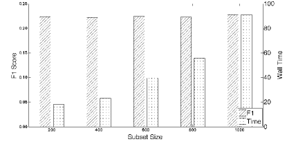
Figure 5: Annotation Performance and Time Cost w.r.t. Subset Sizes

In the experiments above, we choose the parameters for ADML by cross validation and configure the algorithm for optimal annotation performance. On the other hand, the primary motivation for ADML is to save the time cost of metric learning, and the setting of the subset size is a major factor of the overall time cost. Thus it is useful to study how ADML behaves under varying sizes of the subsets. Fig. 5 shows the F1-scores using the metrics learned with different subset sizes. The figure also compares the wall time cost in the training processes. The experiment demonstrates that ADML is stable w.r.t. different data partitions. Thus the algorithm can achieve desirable time efficiency with little sacrifice in the quality of learned distance metrics. Note that this conclusion corroborates the result on the synthetic data shown in Fig. 3.

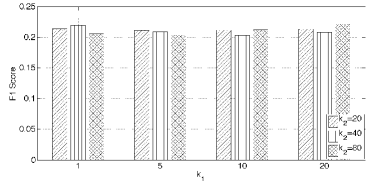
Figure 6: Annotation Performance w.r.t. Within- and Between-class Neighbourhoods

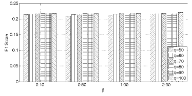
Figure 7: Annotation Performance w.r.t. $\beta$ and subspace dimension

In our experiment, the performance of ADML is relatively stable with respect to the other algorithm settings, including the size of within- and between-class neighbourhoods $k_{1}$ and $k_{2}$, the weight $\beta$ and the subspace dimension $q$ (refer to Section III for detailed explanations of the parameters). Fig. 6 and Fig. 7 show the annotation performance of ADML with varying $k_{1}$, $k_{2}$, $\beta$ and $q$. Note the adjustment of the parameters are grouped into two pairs, $(k_{1},k_{2})$ and $(\beta,q)$, so that we report more behaviours of ADML using less space.

VI CONCLUSION

In this paper, we have proposed a distance metric learning approach that emphasises on encoding categorical information of data. We further derive a part-based solution of the algorithm: the metrics are learned on subsets divided from the entire dataset, and those partial solutions are aggregated into a final distance metric. The aggregated distance metric learning (ADML) technique takes advantage of distributed and parallel computation, and makes metric learning efficient in terms of both time and space usage.

To justify the gain in efficiency, we provide support for the learning quality of ADML in both the theoretical and practical aspects. Theoretically, error bounds are proved showing that the divide-and-conquer technique will give results close to that would be resulted by the performing the discriminative learning method on the entire dataset. Empirically, the properties of the metric learned by ADML have been shown helpful in reflecting the intrinsic relations in the data and helping practical image annotation task. The success of the partition-based processing may also be explained by the theory about the bias-variance trade-off [32]. Learning on a subset, as opposed to the entire data set, may introduce extra bias; on the other hand, ADML can be seen as the weighted combination of results from each subset, which will cause the decrease of variance. Thus, the overall performance may not be affected seriously. Theoretical exploration in this direction make an interesting research subject.

It worth noting that in our empirical study, ADML is implemented using Matlab and the Parallel Computation Toolbox. This implementation facilitates the comparison with other metric learning techniques, but as discussed above, the parallel computation in ADML overlaps those inherited from the Intel’s MKL fundamental subroutines (utilised by Matlab’s low-level operations). ADML can be implemented full-fledged MapReduce architecture, which enables the algorithm to scale up to very large scale and deal with data across multiple nodes of high-performance clusters. A sketch of a distributed implementation is given in Algorithm 1. The algorithm has been tested practically on a cluster. Via OpenMPI, we distributed 32 processes across 8 nodes of Intel Xeon E5 series, each having 8 cores of 2.9 or 3.4GHz. The data are sampled from the distribution as discussed in Subsection V-A. The master process in Algorithm 1 learned metrics from more than 188M samples in 855s, where it aggregated 200k local learned metrics from 31 worker process. In contrast, a sequential implementation of the basic algorithm in Section III took 1718s to learn from 1.88M samples, 1% of the data tackled by the parallel Algorithm 1.

• 

The map-steps, “adml_map()”, compute subset metrics according to (5) (See Section IV). The “adml_reduce” does the aggregation according to (11). The pseudo code is assuming a Message Passing Interface (MPI) as the MapReduce architecture. It is easily convertible to other major programming languages and MapReduce realisation such as Java-Hadoop. Note that for a completely distributed implementation, the procedure can be further decentralised by adjusting the data-accessing in Line 10. The master process may send instructions of retrieving locally stored data, instead of loading the data and sending them to the worker processes.

Algorithm 1 Pseudo code of implementing ADML in a MapReduce framework.

Theorem 1

Proof:

Part I: If $\mathbf{R}=\sum_{k}\mathbf{R}_{k}$ is invertible, we are allowed to write $\hat{\mathbf{W}}=(\sum_{k}\mathbf{R}_{k})^{-1}(\sum_{k}\mathbf{R}_{k})\hat{\mathbf{W}}$. Subtracting $\hat{\mathbf{W}}$ from the aggregation rule (10) gives

$$\mathbf{W}_{A}-\hat{\mathbf{W}}= {\textstyle\mathbf{R}^{-1}\sum_{k=1}^{K}\mathbf{R}_{k}\left(\mathbf{W}_{k}-\hat{\mathbf{W}}\right).}$$

Matrix triangle inequality [23] states that $\|\mathbf{A}_{1}+\mathbf{A}_{2}+\dots\|\leq\|\mathbf{A}_{1}\|+\|\mathbf{A}_{2}\|+\dots$, thus

$$\bigl{\|}\mathbf{W}_{A}-\hat{\mathbf{W}}\bigr{\|} ={\textstyle\Bigl{\|}\mathbf{R}^{-1}\Bigl{(}\sum_{k=1}^{K}\mathbf{R}_{k}\bigl{(}\mathbf{W}_{k}-\hat{\mathbf{W}}\bigr{)}\Bigr{)}\Bigr{\|}}$$

$$\!\!\!\!\!\!\!\!\!\!\!\!\!\!\!\!\!\!\!\!\!\!\!\!\!\!\leq{\textstyle\sum_{k=1}\bigl{\|}\mathbf{R}^{-1}\mathbf{R}_{k}\bigl{(}\mathbf{W}_{k}-\hat{\mathbf{W}}\bigr{)}\bigr{\|}}$$

$$\!\!\!\!\!\!\!\!\!\!\!\!\!\!\!\!\!\!\!\!\!\!\!\!\!\!\leq{\textstyle\max_{k}\bigl{\|}\mathbf{W}_{k}-\hat{\mathbf{W}}\bigr{\|}\times\bigl{\|}\mathbf{R}^{-1}\bigr{\|}{\textstyle\sum_{k=1}^{K}}\left\|\mathbf{R}_{k}\right\|}.$$ (13)

Since for a symmetric matrix $\mathbf{A}$, $\|\mathbf{A}\|=\sqrt{\lambda_{max}(\mathbf{A}^{T}\mathbf{A})}=\lambda_{max}(\mathbf{A})\geq\lambda_{min}(\mathbf{A})$,

$${\textstyle\left\|\mathbf{R}^{-1}\right\|\sum_{k=1}^{K}\left\|\mathbf{R}_{k}\right\|} \leq{\textstyle\frac{1}{\lambda_{min}(\mathbf{R})}\sum_{k}\lambda_{max}(\mathbf{R}_{k})}$$

$${\textstyle\leq\frac{K\max_{k}\{\lambda_{max}(\mathbf{R}_{k})\}}{\lambda_{min}(\mathbf{R})}}=S_{1}.$$ (14)

Combining (13) and (14), we have the first part of Theorem 1. ∎

For the second part, we will need the following lemma.

Lemma 3.

If $\mathbf{A}=\mathbf{A}_{1}+\mathbf{A}_{2}+\dots+\mathbf{A}_{K}$, and $\{\mathbf{A}_{k}\}$ are positive definite matrices, then $\|\mathbf{A}\|\geq K\min_{k}\{\lambda_{min}(\mathbf{A}_{k})\}$.

Proof:

As the sum of positive definite matrices, $\mathbf{A}$ is a positive definite matrix itself. For a positive definite matrix,

$$\mathbf{A}^{T}\mathbf{A}\mathbf{v} =\lambda\mathbf{v}\Leftrightarrow\mathbf{A}\mathbf{v}=\sqrt{\lambda}\mathbf{v}$$

$$\textrm{and }\|\mathbf{A}\| =\lambda_{max}(\mathbf{A})=\max_{\mathbf{v}}\left\{\frac{\mathbf{v}^{T}\mathbf{A}\mathbf{v}}{\|\mathbf{v}\|^{2}}\right\}.$$

Thus it is sufficient to show there exists some $\mathbf{v}$ such that

$$\mathbf{v}^{T}\mathbf{A}\mathbf{v} \geq K\min_{k}\{\lambda_{min}(\mathbf{A}_{k})\}\times\|\mathbf{v}\|^{2}.$$

Since for any $\mathbf{v}$, $\mathbf{v}^{T}\mathbf{A}_{k}\mathbf{v}\geq\lambda_{min}(\mathbf{A}_{k})$, we have

$$\mathbf{v}^{T}\mathbf{A}\mathbf{v} =\sum_{k}\mathbf{v}^{T}\mathbf{A}_{k}\mathbf{v}\geq\sum_{k}\lambda_{min}(\mathbf{A}_{k})\|\mathbf{v}\|^{2}$$

$$\geq K\min_{k}\{\lambda_{min}(\mathbf{A}_{k})\}\times\|\mathbf{v}\|^{2}$$

∎

Lemma 3 leads to the second part of Theorem 1: since $\|\mathbf{R}\|\geq K\min_{k}\{\lambda_{min}(\mathbf{R}_{k})\}$, we can combine $\|\mathbf{R}\|^{-1}\leq\frac{1}{K\min_{k}\{\lambda_{min}(\mathbf{R}_{k})\}}$ with (14) and arrive the desired conclusion.

Theorem 2

Proof:

The aggregation rule (11) indicates

$$\mathbf{W}_{A} =\sum_{k=1}^{K}\mathbf{R}_{k}\mathbf{W}_{k}\mathbf{V}\mathbf{S}^{-1}.$$ (15)

Subtracting $\hat{\mathbf{W}}$ from both sides of (15) gives

$$\|\mathbf{W}_{A}-\hat{\mathbf{W}}\|$$

$$= {\textstyle\|\sum_{k=1}^{K}\mathbf{R}_{k}\mathbf{W}_{k}\mathbf{V}\mathbf{S}^{-1}-\hat{\mathbf{W}}\|}$$

$$\leq {\textstyle\|\sum_{k}\mathbf{R}_{k}(\mathbf{W}_{k}-\hat{\mathbf{W}})\mathbf{V}\mathbf{S}^{-1}\|+\|\sum_{k}\mathbf{R}_{k}\hat{\mathbf{W}}\mathbf{V}\mathbf{S}^{-1}-\hat{\mathbf{W}}\|}$$ (16)

$$\leq {\textstyle\|\mathbf{R}\|\bigl{\|}\sum_{k}(\mathbf{W}_{k}-\hat{\mathbf{W}})\mathbf{V}\mathbf{S}^{-1}\bigr{\|}+\|\mathbf{R}\hat{\mathbf{W}}\mathbf{V}\mathbf{S}^{-1}-\hat{\mathbf{W}}\|}$$ (17)

$$\leq {\textstyle\frac{\lambda_{max}(\mathbf{R})}{\min\{\textrm{diag}(\mathbf{S})\}}\left(1+\sum_{k}\|\mathbf{W}_{k}-\hat{\mathbf{W}}\|\right)+1,}$$ (18)

where (16) and (17) are by the the matrix triangle inequality. The relation (18) translates directly to Theorem 2.∎

Jun Li received his BS degree in computer science and technology from Shandong University, Jinan, China, in 2003, the MSc degree in information and signal processing from Peking University, Beijing, China, in 2006, and the PhD degree in computer science from Queen Mary, University of London, London, UK in 2009. He is currently a research fellow with with the Centre for Quantum Computation and Information Systems and the Faculty of Engineering and Information Technology in the University of Technology, Sydney.

Xu Lin received a BEng degree from South China University of Technology. He is currently with the Shenzhen Institutes of Advanced Technology, Chinese Academy of Sciences, Shenzhen, China, as a visiting student for Human Machine Control. Over the past years, his research interests include machine learning, computer vision.

Xiaoguang Rui has played the key roles in many high impact projects in IBM CRL for industry solutions, and published several papers and filed disclosures/patents. He has received the master and doctoral degrees consecutively in the Department of Electronic Engineering and Information Science (EEIS), University of Science and Technology of China (USTC). His research interests include data mining, and machine learning.

Yong Rui (F’10) is currently a Senior Director and Principal Researcher at Microsoft Research Asia, leading research effort in the areas of multimedia search and mining, knowledge mining, and social computing. From 2010 to 2012, he was Senior Director at Microsoft Asia-Pacific R&D (ARD) Group in charge of China Innovation. From 2008 to 2010, he was Director of Microsoft Education Product in China. From 2006 to 2008, he was a founding member of ARD and its first Director of Strategy. From 1999 to 2006, he was Researcher and Senior Researcher of the Multimedia Collaboration group at Microsoft Research, Redmond, USA. A Fellow of IEEE, IAPR and SPIE, and a Distinguished Scientist of ACM, Rui is recognized as a leading expert in his research areas. He holds 56 issued US and international patents. He has published 16 books and book chapters, and 100+ referred journal and conference papers.

Dacheng Tao (M’07-SM’12) is Professor of Computer Science with the Centre for Quantum Computation and Intelligent Systems and the Faculty of Engineering and Information Technology in the University of Technology, Sydney. He mainly applies statistics and mathematics for data analysis problems in computer vision, data mining, machine learning, multimedia, and video surveillance. He has authored more than 100 scientific articles at top venues including IEEE T-PAMI, T-IP, ICDM, and CVPR. He received the best theory/algorithm paper runner up award in IEEE ICDM’07.

References

- [1] E. P. Xing, A. Y. Ng, M. I. Jordan, and S. Russel, “Distance metric learning with application to clustering with side-information,” in Adv. Neural Info. Proc. Syst. (NIPS), 2003, pp. 505–512.
- [2] N. Shental, T. Hertz, D. Weinshall, and M. Pavel, “Adjustment learning and relevant component analysis,” in Euro. Conf. Comput. Vision (ECCV), 2002, pp. 776–792.
- [3] S. C. H. Hoi, W. Liu, M. R. Lyu, and W. Y. Ma, “Learning distance metrics with contextual constraints for image retrieva,” in Intl. Conf. Comput. Vision Pattern Recog. (CVPR), 2006.
- [4] J. Goldberger, S. Roweis, G. Hinton, , and R. Salakhutdinov, “Neighbourhood components analysis,” in Adv. Neural Info. Proc. Syst. (NIPS), 2005, pp. 513–520.
- [5] K. Q. Weinberger and L. K. Saul, “Distance metric learning for large margin nearest neighbor classification,” J. Mach. Learn. Res., vol. 10, pp. 207–244, 2009.
- [6] S. Fouad, P. Tino, S. Raychaudhury, and P. Schneider, “Incorporating privileged information through metric learning,” IEEE Trans. Neural Networks and Learn. Syst., vol. 24, no. 7, pp. 1086–1098, 2013.
- [7] C. Shen, J. Kim, and L. Wang, “Scalable large-margin Mahalanobis distance metric learning,” IEEE Trans. Neural Networks, vol. 21, no. 9, pp. 1524–1530, 2010.
- [8] S. C. H. Hoi, W. Liu, and S.-F. Chang, “Semi-supervised distance metric learning for collaborative image retrieval and clustering,” ACM Trans. Multimedia Comput. Commun. Appl., vol. 6, no. 3, pp. 18:1–26, 2010.
- [9] F. Kang, R. Jin, and R. Sukthankar, “Correlated label propagation with application to multi-label learning,” in Intl. Conf. Comput. Vision Pattern Recog. (CVPR), 2006.
- [10] J. Dean and S. Ghemawat, “MapReduce: Simplified data processing on large clusters,” ACM Commun., vol. 51, no. 1, pp. 107–113, 2008.
- [11] V. Vapnik, Statistical learning theory. John Wiley & Sons, 1998.
- [12] L. Yang and R. Jin, “Distance metric learning: A comprehensive survey,” Michigan State Univ., Tech. Rep., 2006.
- [13] D.-Y. Yeung and H. Chang, “A kernel approach for semisupervised metric learning,” IEEE Trans. Neural Networks, vol. 18, no. 1, pp. 141–149, 2007.
- [14] C. Domeniconi, J. Peng, and D. Gunopulos, “Locally adaptive metric nearest-neighbor classificaton,” IEEE Trans. Pattern Anal. Mach. Intel., vol. 24, no. 9, pp. 1281–1285, 2002.
- [15] T. Hastie and R. Tibshirani, “Discriminant adaptive nearest neighbor classification,” IEEE Trans. Pattern Anal. Mach. Intel., vol. 18, no. 6, pp. 607–616, 1996.
- [16] L. Grippo, “Convergent online algorithms for supervised learning in neural networks,” IEEE Trans. Neural Networks, vol. 11, no. 6, pp. 1284–1299, 2000.
- [17] J. Davis, B. Kulis, S. Sra, and I. Dhillon, “Information-theoretic metric learning,” in Intl Conf. Mach. Learn. (ICML), 2007, pp. 209–216.
- [18] S. Shalev-shwartz, Y. Singer, and A. Y. Ng, “Online and batch learning of pseudo-metrics,” in Intl Conf. Mach. Learn. (ICML), 2004, pp. 743–750.
- [19] B. Catanzaro, N. Sundaram, and K. Keutzer, “Fast support vector machine training and classification on graphics processors,” in Intl Conf. Mach. Learn. (ICML), 2008, pp. 104–111.
- [20] R. Raina, A. Madhavan, and A. Y. Ng, “Large-scale Deep Unsupervised Learning using Graphics Processors,” in Intl Conf. Mach. Learn. (ICML), 2009, pp. 873–880.
- [21] C.-T. Chu, S. K. Kim, Y.-A. Lin, Y. Yu, G. Bradski, A. Y. Ng, and K. Olukotun, “Map-reduce for machine learning on multicore,” in Adv. Neural Info. Proc. Syst. (NIPS), 2007, pp. 281–288.
- [22] N. Lin and R. Xi, “Aggregated estimating equation estimation,” Statistics and Its Interface, vol. 4, pp. 73–84, 2011.
- [23] R. Horn and C. Johnson, Matrix Analysis. Cambridge University Press, 1990. [Online]. Available: http://www.citeulike.org/user/Borelli/article/669570
- [24] A. Smeulders, M. Worring, S. Santini, A. Gupta, and R. Jain, “Content-based image retrieval at the end of the early years,” IEEE Trans. Pattern Anal. Mach. Intel., vol. 22, no. 12, pp. 1349–1380, 2000.
- [25] T.-S. Chua, J. Tang, R. Hong, H. Li, Z. Luo, , and Y.-T. Zheng, “NUS-WIDE: A real-world web image database from National University of Singapore,” in ACM Intl. Conf. Image and Video Retrieval, 2009, pp. 48:1–48:9.
- [26] J. Jeon, V. Lavrenko, and R. Manmatha, “Automatic image annotation and retrieval using cross-media relevance models,” in ACM SIG Info. Retrieval (SIGIR), 2003.
- [27] C. J. Van Rijsbergen, Information Retrieval (2nd ed.). Butter-worth, 1979.
- [28] A. Makadia, V. Pavlovic, and S. Kumar, “A new baseline for image annotation,” in Euro. Conf. Comput. Vision (ECCV), 2008, pp. 316–329.
- [29] M. Guillaumin, T. Mensink, J. Verbeek, and C. Schmid, “TagProp: Discriminative metric learning in nearest neighbor models for image auto-annotation,” in Intl. Conf. Comput. Vision, 2009, pp. 309–316.
- [30] G. E. Blelloch and B. M. Maggs, “A brief overview of parallel algorithms,” http://http://www.cs.cmu.edu/~scandal/html-papers/short/short.html.
- [31] M. Tahir and A. Bouridane, “An FPGA based coprocessor for cancer classification using nearest neighbour classifier,” in Intl. Conf. Acoust., Speech and Signal Proc. (ICASSP), 2006.
- [32] T. Hastie, R. Tibshirani, and J. Friedman, The Elements of Statistical Learning, corrected ed. Springer, 2003. [Online]. Available: http://www.citeulike.org/user/gyuli/article/161814