Cosmological data favor Galileon ghost condensate over $\Lambda$CDM

Abstract

We place observational constraints on the Galileon ghost condensate model, a dark energy proposal in cubic-order Horndeski theories consistent with the gravitational-wave event GW170817. The model extends the covariant Galileon by taking an additional higher-order field derivative $X^{2}$ into account. This allows for the dark energy equation of state $w_{\rm DE}$ to access the region $-2<w_{\rm DE}<-1$ without ghosts. Indeed, this peculiar evolution of $w_{\rm DE}$ is favored over that of the cosmological constant $\Lambda$ from the joint data analysis of cosmic microwave background (CMB) radiation, baryonic acoustic oscillations (BAOs), supernovae type Ia (SNIa) and redshift-space distortions (RSDs). Furthermore, our model exhibits a better compatibility with the CMB data over the $\Lambda$-cold-dark-matter ($\Lambda$CDM) model by suppressing large-scale temperature anisotropies. The CMB temperature and polarization data lead to an estimation for today’s Hubble parameter $H_{0}$ consistent with its direct measurements at 2$\sigma$. We perform a model selection analysis by using several methods and find a statistically significant preference of the Galileon ghost condensate model over $\Lambda$CDM.

I Introduction

The late-time cosmic acceleration has been firmly confirmed by several independent observations including SNIa SN1 ; SN2 ; Betoule , CMB WMAP ; Planck1 ; Planck2 , and BAOs Eisen ; BAO1 ; BAO2 . Although the cosmological constant $\Lambda$ is the simplest candidate for the source of this phenomenon, it is generally plagued by the problem of huge difference between the observed dark energy scale and the vacuum energy associated with particle physics Weinberg . In the $\Lambda$CDM model, there have been also tensions for today’s Hubble expansion rate $H_{0}$ constrained from the Planck CMB data Planck1 and its direct measurements at low redshifts Riess18 .

In the presence of a scalar field $\phi$, the negative pressure arising from its potential or nonlinear kinetic energy can drive the cosmic acceleration. If we allow for derivative interactions and nonminimal couplings to gravity, Horndeski theories Horndeski are the most general scalar-tensor theories with second-order equations of motion ensuring the absence of Ostrogradski instabilities Ho1 ; Ho2 . The gravitational-wave event GW170817 GW170817 together with its electromagnetic counterpart Goldstein show that the speed of gravity $c_{t}$ is close to that of light with the relative difference $\sim 10^{-15}$. If we strictly demand that $c_{t}=1$, the Horndeski Lagrangian is of the form $L_{\rm H}=G_{4}(\phi)R+G_{2}(\phi,X)+G_{3}(\phi,X)\square\phi$, where $R$ is the Ricci scalar, $G_{4}$ is a function of $\phi$, and $G_{2},G_{3}$ depend on both $\phi$ and $X=\partial_{\mu}\phi\partial^{\mu}\phi$ GWcon1 ; GWcon2 ; GWcon3 ; GWcon4 ; GWcon5 .

Theories with the nonminimal coupling $G_{4}(\phi)R$ include $f(R)$ gravity and Brans-Dicke theories, but we have not yet found any observational signatures for supporting nonminimally coupled dark energy models over the cosmological constant. The minimally coupled quintessence and k-essence with the Lagrangian $L=M_{\rm pl}^{2}R/2+G_{2}(\phi,X)$, where $M_{\rm pl}$ is the reduced Planck mass, predicts $w_{\rm DE}>-1$ under the absence of ghosts, but there has been no significant observational evidence that these models are favored over $\Lambda$CDM.

The cubic-order Horndeski Lagrangian $G_{3}(\phi,X)\square\phi$ allows an interesting possibility for realizing $w_{\rm DE}<-1$ without ghosts. In cubic Galileons with the Lagrangian $L=M_{\rm pl}^{2}R/2+a_{1}X+3a_{3}X\square\phi$ Nicolis ; Galileons , where $a_{1}$ and $a_{3}$ are constants, there exists a tracker solution along which $w_{\rm DE}=-2$ during the matter era DT10 . This behavior of $w_{\rm DE}$ is in tension with the joint data analysis of SNIa, CMB, and BAO NDT10 . The dominance of cubic Galileons as a dark energy density at low redshifts also leads to the enhancement of perturbations incompatible with measurements of the cosmic growth history Renk ; Peirone .

The above problems of Galileons are alleviated by taking a scalar potential $V(\phi)$ Ali ; KTD15 or a nonlinear term of $X$ in $G_{2}(\phi,X)$ into account Kase18 . In particular, the latter model can lead to $w_{\rm DE}$ in the range $-2<w_{\rm DE}<-1$. Moreover, the Galileon is not necessarily the main source for late-time cosmic acceleration in this case, so it should be compatible with cosmic growth measurements. In this letter, we show that the cubic Galileon model with a nonlinear term in $X$ exhibits a novel feature of being observationally favored over $\Lambda$CDM.

II Model

We study the Galileon ghost condensate (GGC) model given by the action

$${\cal S}=\int{\rm d}^{4}x\sqrt{-g}\left[\frac{M_{\rm pl}^{2}}{2}R+a_{1}X+a_{2}X^{2}+3a_{3}X\square\phi\right]+{\cal S}_{M},$$ (1)

where $a_{1,2,3}$ are constants. For the matter action ${\cal S}_{M}$, we consider perfect fluids minimally coupled to gravity. The existence of term $a_{2}X^{2}$ leads to the modified evolution of $w_{\rm DE}$ and different cosmic growth history compared to those of the cubic Galileon (which corresponds to $a_{2}=0$). The ghost condensate model Arkani can be recovered by taking the limit $a_{3}\to 0$ in Eq. (1).

On the flat Friedmann-Lemaitre-Robertson-Walker (FLRW) background given by the line element ${\rm d}s^{2}=-{\rm d}t^{2}+a^{2}(t)\delta_{ij}{\rm d}x^{i}{\rm d}x^{j}$, we consider nonrelativistic matter (density $\rho_{m}$ with vanishing pressure) and radiation (density $\rho_{r}$ and pressure $P_{r}=\rho_{r}/3$) for the action ${\cal S}_{M}$. To discuss the background cosmological dynamics, it is convenient to introduce the dimensionless variables

$$x_{1}=-\frac{a_{1}\dot{\phi}^{2}}{3M_{\rm pl}^{2}H^{2}}\,,\quad x_{2}=\frac{a_{2}\dot{\phi}^{4}}{M_{\rm pl}^{2}H^{2}}\,,\quad x_{3}=\frac{6a_{3}\dot{\phi}^{3}}{M_{\rm pl}^{2}H}\,,$$ (2)

where $H=\dot{a}/a$, and a dot represents the derivative with respect to the cosmic time $t$. Then, the Friedmann equation can be expressed in the form $\Omega_{m}+\Omega_{r}+\Omega_{\rm DE}=1$  where $\Omega_{m}=\rho_{m}/(3M_{\rm pl}^{2}H^{2})$, $\Omega_{r}=\rho_{r}/(3M_{\rm pl}^{2}H^{2})$, and

$$\Omega_{\rm DE}=x_{1}+x_{2}+x_{3}\,.$$ (3)

The variables $x_{1}$, $x_{2}$, $x_{3}$, and $\Omega_{r}$ correspond to density parameters associated with the Lagrangians $a_{1}X$, $a_{2}X^{2}$, $3a_{3}X\square\phi$, and radiation, respectively. Equation (3) evaluated today allows us to eliminate one free parameter, leaving the model with two extra parameters compared to $\Lambda$CDM.

The dynamical system can be expressed in the form

$$x_{1}^{\prime}=2x_{1}(\epsilon_{\phi}-h)\,,\qquad x_{2}^{\prime}=2x_{2}(2\epsilon_{\phi}-h)\,,$$

$$x_{3}^{\prime}=x_{3}(3\epsilon_{\phi}-h)\,,\qquad\Omega_{r}^{\prime}=-2\Omega_{r}(2+h)\,,$$ (4)

where $\epsilon_{\phi}=\ddot{\phi}/(H\dot{\phi})$, $h=\dot{H}/H^{2}$, and a prime represents a derivative with respect to ${\cal N}=\ln a$. The explicit expressions of $\epsilon_{\phi}$ and $h$ are given in Eqs. (4.16) and (4.17) of Ref. Kase18 (with $x_{4}=0$). The dark energy equation of state is

$$w_{\rm DE}=\frac{3x_{1}+x_{2}-\epsilon_{\phi}x_{3}}{3(x_{1}+x_{2}+x_{3})}\,.$$ (5)

On the future de Sitter fixed point we have $\Omega_{\rm DE}=1$, and $w_{\rm DE}=-1$ with $\epsilon_{\phi}=0$, so there are two relations $x_{1}^{\rm dS}=-2+x_{3}^{\rm dS}/2$ and $x_{2}^{\rm dS}=3-3x_{3}^{\rm dS}/2$. Even though $x_{1}^{\rm dS}$ is negative for $x_{3}^{\rm dS}\ll 1$, the ghost can be avoided by the positive $x_{2}^{\rm dS}$ term.

If the condition $x_{3}\gg\{|x_{1}|,x_{2}\}$ is satisfied in the early cosmological epoch, we have $w_{\rm DE}\simeq-\epsilon_{\phi}/3\simeq 1/4-\Omega_{r}/12>0$. On the other hand, in the limit $x_{2}\to 0$, there exists a tracker solution satisfying the relation $x_{3}=-2x_{1}$ (or equivalently, $\epsilon_{\phi}=-h$) DT10 ; Kase18 . In this case, Eq. (5) reduces to $w_{\rm DE}=-1+2h/3$ and hence $w_{\rm DE}\simeq-2$ during the matter era. The existence of positive $x_{2}$ can lead to $w_{\rm DE}$ larger than $-2$, so the approach to the tracker is prevented by the term $a_{2}X^{2}$. Indeed, after $x_{2}$ catches up with $x_{3}$, the solutions tend to approach the de Sitter attractor with $x_{3}$ subdominant to $|x_{1}|$ and $x_{2}$ at low redshifts Kase18 . In this way, the background dynamics temporally entering the region $-2<w_{\rm DE}<-1$ can be realized by the model (1) with $a_{2}\neq 0$.

III Cosmological perturbations

For the GGC model (1), the propagation of tensor perturbations is the same as that in General Relativity (GR). As for scalar perturbations, we consider the perturbed line element on the flat FLRW background:

$${\rm d}s^{2}=-\left(1+2\Psi\right){\rm d}t^{2}+a^{2}(t)\left(1-2\Phi\right)\delta_{ij}{\rm d}x^{i}{\rm d}x^{j}\,,$$ (6)

where $\Psi$ and $\Phi$ are gravitational potentials. In Fourier space with the coming wavenumber $k$, we relate $\Psi$ and $\Psi+\Phi$ with the total matter density perturbation $\rho\Delta=\sum_{i}\rho_{i}\Delta_{i}$ (where $i=m,r,...$), as Amen07 ; Ber08 ; Pogo10

$$-k^{2}\Psi=4\pi G_{\rm N}a^{2}\mu(a,k)\rho\Delta\,,$$ (7)

$$-k^{2}(\Psi+\Phi)=8\pi G_{\rm N}a^{2}\Sigma(a,k)\rho\Delta\,,$$ (8)

where $G_{\rm N}=(8\pi M_{\rm pl}^{2})^{-1}$ is the Newtonian gravitational constant. The dimensionless quantities $\mu$ and $\Sigma$ characterize the effective gravitational couplings felt by matter and light, respectively. Applying the quasi-static approximation Pola00 ; DKT for perturbations deep inside the Hubble radius to the model (1), it follows that Kase18

$$\mu=\Sigma=1+\frac{x_{3}^{2}}{Q_{s}c_{s}^{2}(2-x_{3})^{2}}\,,$$ (9)

where

$$Q_{s} = \frac{3(4x_{1}+8x_{2}+4x_{3}+x_{3}^{2})}{(2-x_{3})^{2}}\,,$$ (10)

$$c_{s}^{2} = \frac{2(1+3\epsilon_{\phi})x_{3}-x_{3}^{2}-4h-6\Omega_{m}-8\Omega_{r}}{3(4x_{1}+8x_{2}+4x_{3}+x_{3}^{2})}\,.$$ (11)

To avoid ghosts and Laplacian instabilities, we require that $Q_{s}>0$ and $c_{s}^{2}>0$. Then, for $x_{3}\neq 0$, $\mu$ and $\Sigma$ are larger than 1, so both $\Psi$ and $\Psi+\Phi$ are enhanced compared to those in GR. Since $\mu=\Sigma$, there is no gravitational slip ($\Psi=\Phi$). For the sub-horizon perturbations, the matter density contrast $\Delta$ approximately obeys

$$\ddot{\Delta}+2H\dot{\Delta}-4\pi G_{\rm N}\mu\rho\Delta=0\,,$$ (12)

so the cosmic growth rate is larger than that in GR. In the likelihood analysis, we solve full perturbation equations without resorting to the quasi-static approximation.

IV Methodology of cosmological probes

To confront the GGC model with observations, we use the Planck 2015 data of CMB temperature anisotropies and polarizations (Planck1, ; Planck2, ). For the Planck likelihood, we also vary the nuisance parameters exploited to model foregrounds as well as instrumental and beam uncertainties. We consider the former dataset in combination with data from the CMB lensing reconstruction Ade:2015zua , to which we refer as “Planck+Lensing”. We include the BAO data from the 6dF galaxy survey (BAO1, ) and the SDSS DR7 main galaxy sample (BAO2, ). Furthermore, we employ the combined BAO and RSD data from the SDSS DR12 consensus release Alam , together with the JLA SNIa sample Betoule . The latter dataset is called “PBRS”.

We modify the public available Einstein-Boltzmann code EFTCAMB Hu:2013twa ; Raveri:2014cka by implementing a background solver and mapping relations for the chosen model following the prescription in Refs. Gubitosi:2012hu ; Bloomfield:2012ff ; Gleyzes:2013ooa ; Frusciante:2016xoj . The built-in stability module allows us to identify the viable parameter space by imposing the two stability conditions $Q_{s}>0$ and $c_{s}^{2}>0$. These results will be used to set priors for the data analysis. We impose flat priors on the initial values of two model parameters: $x_{1}^{(i)}\in[-10,10]\times 10^{-16}$, $x_{3}^{(i)}\in[-10,10]\times 10^{-9}$ at the redshift $z=10^{5}$. We performed a test simulation in which the prior ranges are increased by one order of magnitude and found no difference for the likelihood results.

V Observational constraints

In Tables 1 and 2, we show today’s values $x_{1}^{(0)},x_{2}^{(0)},x_{3}^{(0)}$ and $H_{0}$, $\sigma_{8}^{(0)}$, $\Omega_{m}^{(0)}$ constrained from the Planck and PBRS datasets, together with bounds on the latter three parameters in $\Lambda$CDM. In Fig. 1, we also plot two-dimensional observational bounds on six parameters by including the Planck+Lensing data as well. In GGC, the Planck data alone lead to higher values of $H_{0}$ than that in $\Lambda$CDM. The former model is consistent with the Riess et al. bound $H_{0}=73.48\pm 1.66$ km s^-1 Mpc^-1 derived by direct measurements of $H_{0}$ using Cepheids Riess18 . With the PBRS and CMB lensing datasets, we find that the bounds on $H_{0}$, $\sigma_{8}^{(0)}$ and $\Omega_{m}^{(0)}$ are compatible between GGC and $\Lambda$CDM. We do not include the data of direct measurements of $H_{0}$ and weak lensing, as they can be affected by the statistical analysis Efstathiou and nonlinear perturbation dynamics Hildebrandt:2016iqg , respectively.

Parameter	Planck	PBRS
$x_{1}^{(0)}$	$-1.27^{+0.22}_{-0.15}\,(-1.26)$	$-1.35^{+0.1}_{-0.07}\,(-1.27)$
$x_{2}^{(0)}$	$1.70^{+0.45}_{-0.73}\,(1.64)$	$1.95^{+0.18}_{-0.31}\,(1.74)$
$x_{3}^{(0)}$	$0.28^{+0.5}_{-0.3}\,(0.34)$	$0.09^{+0.2}_{-0.1}\,(0.23)$

Table 1: Marginalized values of the model parameters $x_{1}^{(0)},x_{2}^{(0)},x_{3}^{(0)}$ and their $95\%$ CL bounds, obtained by Planck and PBRS datasets. In parenthesis we show maximum likelihood values.

Parameter	Case	Planck	PBRS
	GGC	$69.3^{+3.6}_{-3.0}\,(70)$	$68.1\pm 1.1\,(68.4)$
$H_{0}$
	$\Lambda$CDM	$67.9\pm 2.0\,(67.6)$	$68\pm 1\,(68)$
	GGC	$0.86\pm 0.04\,(0.87)$	$0.84\pm 0.03$  (0.85)
$\sigma_{8}^{(0)}$
	$\Lambda$CDM	$0.841\pm 0.03\,(0.83)$	$0.84\pm 0.03\,(0.84)$
	GGC	$0.30\pm 0.04\,(0.28)$	$0.305\pm 0.01$ (0.30)
$\Omega_{m}^{(0)}$
	$\Lambda$CDM	$0.30\pm 0.03\,(0.31)$	$0.31\pm 0.01\,(0.31)$

Table 2: Marginalized values of $H_{0}$, $\sigma_{8}^{(0)}$, $\Omega_{m}^{(0)}$ and their $95\%$ CL bounds.

The values of $x_{1}^{(0)}$ and $x_{2}^{(0)}$ constrained from the data are of order 1, with $x_{1}^{(0)}<0$ and $x_{2}^{(0)}>0$. We find the upper limit $x_{3}^{(0)}<0.118$ (68 % CL) from the PBRS data. This bound mostly arises from the fact that the dominance of $x_{3}$ over $x_{2}$ at low redshifts leads to the enhanced Integrated Sachs-Wolfe (ISW) effect on CMB temperature anisotropies. The most stringent constraints on model parameters are obtained with the Planck+Lensing datasets. In Fig. 2, we plot the CMB TT power spectra for GGC as well as for $\Lambda$CDM and cubic Galileons (G3), given by the best-fit to the Planck data. The G3 model corresponds to $x_{2}=0$, so that the Galileon density is the main source for cosmic acceleration. In this case, the TT power spectrum for the multipoles $l<{\cal O}(10)$ is strongly enhanced relative to $\Lambda$CDM and this behavior is disfavored from the Planck data Peirone .

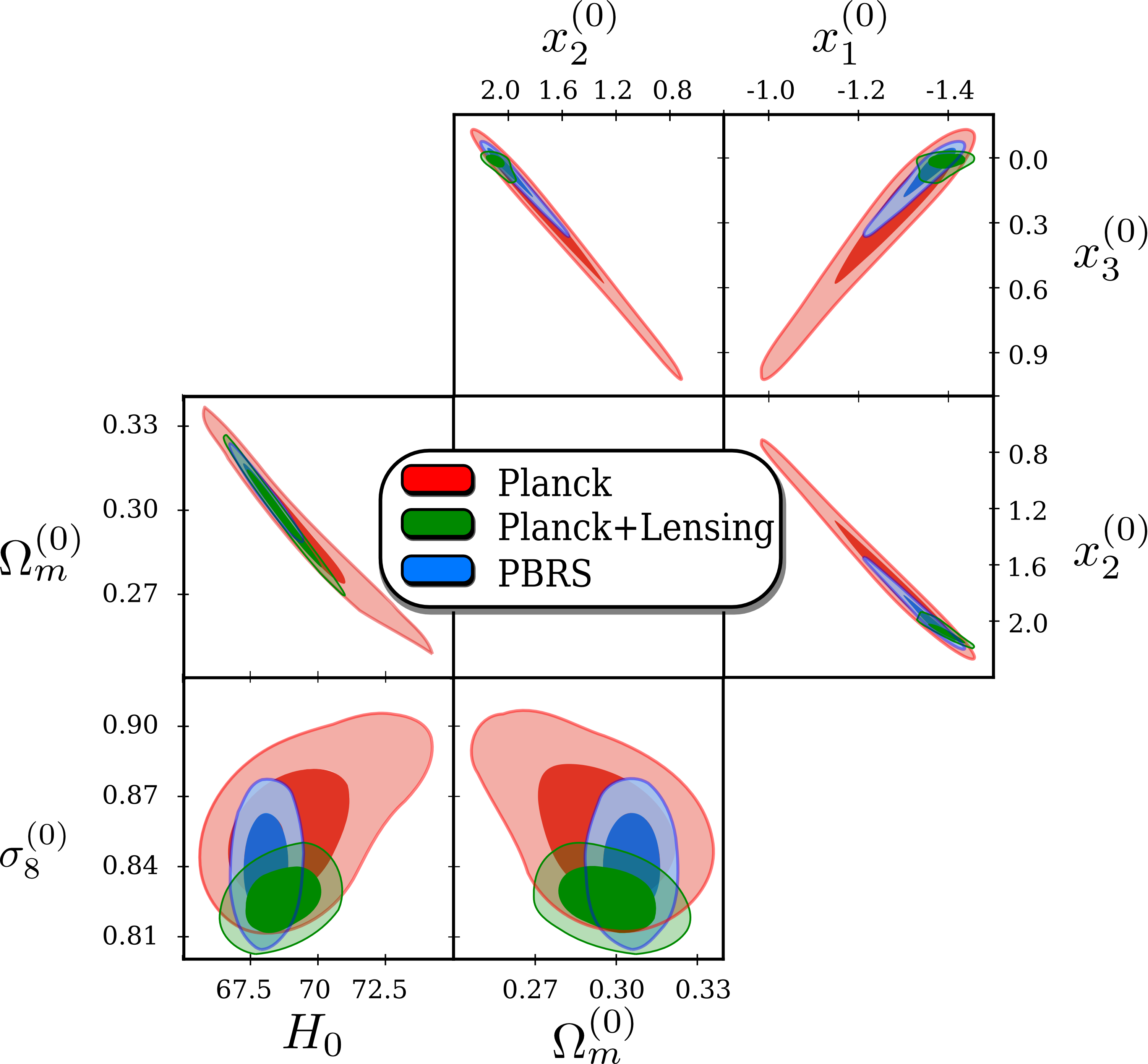
Figure 1: Joint marginalised constraints (68 % and 95 % CLs) on six model parameters $x_{1}^{(0)},x_{2}^{(0)},x_{3}^{(0)},H_{0},\sigma_{8}^{(0)},\Omega_{m}^{(0)}$ obtained with the Planck, Planck+Lensing, and PBRS datasets.

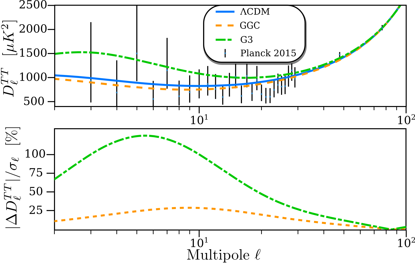
Figure 2: Top panel: Best-fit CMB temperature-temperature (TT) power spectra $D_{\ell}^{\rm TT}=\ell(\ell+1)/2\pi C_{\ell}^{\rm TT}$ at low multipoles $\ell$ for $\Lambda$CDM, GGC, and G3 (cubic Galileons), as obtained in the analysis of the Planck dataset. The best-fit values for G3 are taken from Ref. Peirone . For comparison, we plot the data points from Planck 2015. Bottom panel: Relative difference of the best-fit TT power spectra, in units of cosmic variance $\sigma_{\ell}=\sqrt{2/(2\ell+1)}C_{\ell}^{\Lambda{\rm CDM}}$.

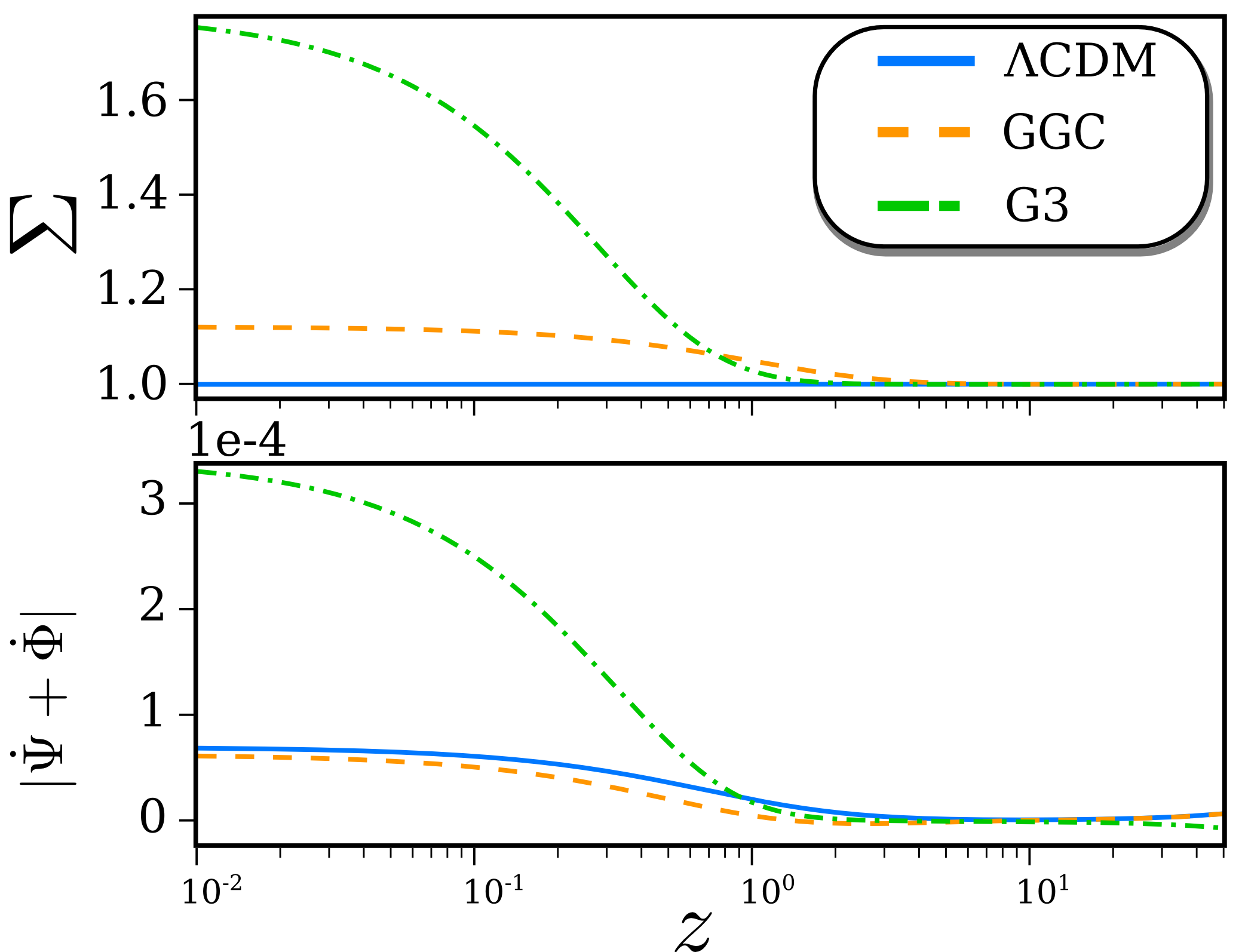
Figure 3: Best-fit evolution of $\Sigma$ (top) and $|\dot{\Psi}+\dot{\Phi}|$ (bottom) versus $z$ at $k=0.01$ Mpc^-1 for $\Lambda$CDM, GGC, and G3 derived with the PBRS dataset.

Figure 4: Best-fit evolution of $w_{\rm DE}$ versus $z$ for $\Lambda$CDM, GGC, and G3 derived with the PBRS dataset.

In GGC, the $a_{2}X^{2}$ term in (1) can avoid the dominance of $x_{3}$ over $x_{2}$ around today. Even if $x_{3}^{(0)}\ll x_{2}^{(0)}$, the cubic Galileon gives rise to an interesting contribution to the CMB TT spectrum. As we see in Fig. 2, the best-fit GGC model is in better agreement with the Planck data relative to $\Lambda$CDM by suppressing large-scale ISW tails. Taking the limit $x_{3}^{(0)}\to 0$, the TT spectrum approaches the one in $\Lambda$CDM. The TT spectrum of G3 in Fig. 2 can be recovered by taking the limit $x_{3}^{(0)}\gg x_{2}^{(0)}$.

In Fig. 3, we depict the evolution of $\Sigma$ and $|\dot{\Psi}+\dot{\Phi}|$ for GGC, G3 and $\Lambda$CDM, obtained from the PBRS best-fit. In G3, the large growth of $\Sigma$ from 1 leads to the enhanced ISW effect on CMB anisotropies determined by the variation of $\Psi+\Phi$ at low redshifts. For the best-fit GGC, the deviation of $\Sigma$ from 1 is less significant, with $\dot{\Psi}+\dot{\Phi}$ closer to 0. In the latter case, the TT spectrum is suppressed with respect to $\Lambda$CDM. This is why the intermediate value of $x_{3}^{(0)}$ around 0.1 with $x_{2}^{(0)}={\cal O}(1)$ exhibits the better compatibility with the CMB data relative to $\Lambda$CDM.

As we see in Fig. 4, the best-fit GGC corresponds to the evolution of $w_{\rm DE}$ approaching the asymptotic value $-1$ from the region $-2<w_{\rm DE}<-1$. This overcomes the problem of G3 in which the $w_{\rm DE}=-2$ behavior during the matter era is inconsistent with the CMB+BAO+SNIa data NDT10 . This nice feature of $w_{\rm DE}$ in GGC again comes from the combined effect of $x_{2}$ and $x_{3}$.

VI Model selection

The GGC model has two extra parameters with respect to $\Lambda$CDM, to allow for a better fit to the data. In order to determine whether GGC is favored over $\Lambda$CDM, we make use of the Deviance Information Criterion (DIC) RSSB :

$${\rm DIC}=\chi^{2}_{\rm eff}(\hat{\theta})+2p_{\rm D}\,,$$ (13)

where $\chi^{2}_{\rm eff}(\hat{\theta})=-2\ln\mathcal{L}(\hat{\theta})$ with $\hat{\theta}$ being parameters maximizing the likelihood function $\mathcal{L}$, and $p_{\rm D}=\bar{\chi}^{2}_{\rm eff}({\theta})-\chi^{2}_{\rm eff}(\hat{\theta})$. Here, the bar denotes an average over the posterior distribution. We observe that the DIC accounts for both the goodness of fit, $\chi^{2}_{\rm eff}(\hat{\theta})$, and for the Bayesian complexity of the model, $p_{\rm D}$, which disfavors more complex models. For the purpose of model comparisons, we compute

$$\Delta{\rm DIC}={\rm DIC}_{\rm GGC}-{\rm DIC}_{\Lambda{\rm CDM}},$$ (14)

from which we infer that a negative (positive) $\Delta{\rm DIC}$ would support GGC ($\Lambda$CDM).

We also consider the Bayesian evidence factor ($\log_{10}B$) along the line of Refs. Heavens:2017afc ; DeBernardis:2009di to quantify the support for GGC over $\Lambda$CDM. A positive value of $\Delta\log_{10}B$ indicates a statistical preference for the extended model and a strong preference is defined for $\Delta\log_{10}B>2$.

Dataset	$\Delta\chi_{\rm eff}^{2}$	$\Delta{\rm DIC}$	$\Delta\log_{10}B$
Planck	$-4.8$	$-2.5$	4.4
PBRS	$-2.8$	$-0.6$	5.1
Planck+Lensing	$-0.9$	0.80	1.6

Table 3: Model comparisons through the obtained values of $\Delta\chi_{\rm eff}^{2}$, $\Delta{\rm DIC}$ and $\Delta\log_{10}B$ using $\Lambda$CDM as reference.

In Table 3, we list the values of $\Delta\chi_{\rm eff}^{2}$, $\Delta{\rm DIC}$ and $\Delta\log_{10}B$ computed with respect to $\Lambda$CDM for each dataset considered in this analysis. For Planck and PBRS both $\Delta{\rm DIC}$ and $\Delta\log_{10}B$ exhibit significant preferences for GGC over $\Lambda$CDM. This suggests that not only the CMB data but also the combination of BAO, SNIa, RSD datasets favors the cosmological dynamics of GGC like the best-fit case shown in Figs. 3 and 4. With the Planck+Lensing data the $\chi_{\rm eff}^{2}$ and Bayesian factor exhibit slight preferences for GGC, while the DIC mildly favours $\Lambda$CDM. The model selection analysis with the CMB lensing data does not give a definite conclusion for the preference of models. We note that, among the likelihoods used in our analysis, the CMB lensing alone assumes $\Lambda$CDM as a fiducial model Ade:2015zua . This might source a bias towards the latter.

VII Conclusion

We have shown that, according to the two information criteria, GGC is significantly favoured over $\Lambda$CDM with the PBRS datasets. This property holds even with two additional model parameters than those in $\Lambda$CDM. According to our knowledge, there are no other scalar-tensor dark energy models proposed so far showing such novel properties. This surprising result is attributed to the properties that, for $x_{3}^{(0)}\ll x_{2}^{(0)}={\cal O}(1)$, (i) suppressed ISW tails relative to $\Lambda$CDM can be generated, and (ii) $w_{\rm DE}$ can be in the region $-2<w_{\rm DE}<-1$ at low redshifts. The GGC model deserves for being tested further in future observations of WL, ISW-galaxy cross-correlations, and gravitational waves.

References

- (1) A. G. Riess et al., Astron. J. 116, 1009 (1998).
- (2) S. Perlmutter et al., Astrophys. J. 517, 565 (1999).
- (3) M. Betoule et al., Astron. Astrophys. 568, A22 (2014).
- (4) D. N. Spergel et al., Astrophys. J. Suppl. 148, 175 (2003).
- (5) P. A. R. Ade et al., Astron. Astrophys. 594, A13 (2016).
- (6) N. Aghanim et al., Astron. Astrophys. 594, A11 (2016).
- (7) D. J. Eisenstein et al., Astrophys. J. 633, 560 (2005)
- (8) F. Beutler et al., Mon. Not. Roy. Astron. Soc. 416, 3017 (2011).
- (9) A. J. Ross et al., Mon. Not. Roy. Astron. Soc. 449, 835 (2015).
- (10) S. Weinberg, Rev. Mod. Phys. 61, 1 (1989).
- (11) A. G. Riess et al., Astrophys. J. 861, no. 2, 126 (2018).
- (12) G. W. Horndeski, Int. J. Theor. Phys. 10, 363 (1974).
- (13) C. Deffayet, X. Gao, D. A. Steer and G. Zahariade, Phys. Rev. D 84, 064039 (2011).
- (14) T. Kobayashi, M. Yamaguchi and J. Yokoyama, Prog. Theor. Phys. 126, 511 (2011).
- (15) B. P. Abbott et al., Phys. Rev. Lett. 119, 161101 (2017).
- (16) A. Goldstein et al., Astrophys. J. 848, L14 (2017).
- (17) T. Baker, E. Bellini, P. G. Ferreira, M. Lagos, J. Noller and I. Sawicki, Phys. Rev. Lett. 119, 251301 (2017).
- (18) P. Creminelli and F. Vernizzi, Phys. Rev. Lett. 119, 251302 (2017).
- (19) J. Sakstein and B. Jain, Phys. Rev. Lett. 119, 251303 (2017).
- (20) J. M. Ezquiaga and M. Zumalacarregui, Phys. Rev. Lett. 119, 251304 (2017).
- (21) L. Amendola, M. Kunz, I. D. Saltas and I. Sawicki, Phys. Rev. Lett. 120, 131101 (2018).
- (22) A. Nicolis, R. Rattazzi and E. Trincherini, Phys. Rev. D 79, 064036 (2009).
- (23) C. Deffayet, G. Esposito-Farese and A. Vikman, Phys. Rev. D 79, 084003 (2009).
- (24) A. De Felice and S. Tsujikawa, Phys. Rev. Lett. 105, 111301 (2010).
- (25) S. Nesseris, A. De Felice and S. Tsujikawa, Phys. Rev. D 82, 124054 (2010).
- (26) J. Renk, M. Zumalacaregui, F. Montanari and A. Barreira, JCAP 1710, 020 (2017).
- (27) S. Peirone, N. Frusciante, B. Hu, M. Raveri and A. Silvestri, Phys. Rev. D 97, 063518 (2018).
- (28) A. Ali, R. Gannouji, M. W. Hossain and M. Sami, Phys. Lett. B 718, 5 (2012)
- (29) R. Kase, S. Tsujikawa and A. De Felice, Phys. Rev. D 93, 024007 (2016).
- (30) R. Kase and S. Tsujikawa, Phys. Rev. D 97, 103501 (2018).
- (31) N. Arkani-Hamed, H. C. Cheng, M. A. Luty and S. Mukohyama, JHEP 0405, 074 (2004).
- (32) L. Amendola, M. Kunz and D. Sapone, JCAP 0804, 013 (2008).
- (33) E. Bertschinger and P. Zukin, Phys. Rev. D 78, 024015 (2008).
- (34) L. Pogosian, A. Silvestri, K. Koyama and G. B. Zhao, Phys. Rev. D 81, 104023 (2010).
- (35) B. Boisseau, G. Esposito-Farese, D. Polarski and A. A. Starobinsky, Phys. Rev. Lett. 85, 2236 (2000).
- (36) A. De Felice, T. Kobayashi and S. Tsujikawa, Phys. Lett. B 706, 123 (2011).
- (37) P. A. R. Ade et al. [Planck Collaboration], Astron. Astrophys. 594, A15 (2016).
- (38) S. Alam et al., Mon. Not. Roy. Astron. Soc. 470, 2617 (2017).
- (39) B. Hu, M. Raveri, N. Frusciante and A. Silvestri, Phys. Rev. D 89, 103530 (2014).
- (40) M. Raveri, B. Hu, N. Frusciante and A. Silvestri, Phys. Rev. D 90, 043513 (2014)
- (41) G. Gubitosi, F. Piazza and F. Vernizzi, JCAP 1302, 032 (2013).
- (42) J. K. Bloomfield, E. E. Flanagan, M. Park and S. Watson, JCAP 1308, 010 (2013).
- (43) J. Gleyzes, D. Langlois, F. Piazza and F. Vernizzi, JCAP 1308, 025 (2013).
- (44) N. Frusciante, G. Papadomanolakis and A. Silvestri, JCAP 1607, 018 (2016).
- (45) G. Efstathiou, Mon. Not. Roy. Astron. Soc. 440, 1138 (2014).
- (46) H. Hildebrandt et al., Mon. Not. Roy. Astron. Soc. 465, 1454 (2017).
- (47) D. J. Spiegelhalter, N. G. Best, B. P. Carlin, and A. van der Linde, J. Roy. Statist. Soc. B 76, 485 (2014).
- (48) A. Heavens et al., arXiv:1704.03472.
- (49) F. De Bernardis, T. D. Kitching, A. Heavens and A. Melchiorri, Phys. Rev. D 80, 123509 (2009).