Spectral Coarsening of Geometric Operators

Abstract.

We introduce a novel approach to measure the behavior of a geometric operator before and after coarsening. By comparing eigenvectors of the input operator and its coarsened counterpart, we can quantitatively and visually analyze how well the spectral properties of the operator are maintained. Using this measure, we show that standard mesh simplification and algebraic coarsening techniques fail to maintain spectral properties. In response, we introduce a novel approach for spectral coarsening. We show that it is possible to significantly reduce the sampling density of an operator derived from a 3D shape without affecting the low-frequency eigenvectors. By marrying techniques developed within the algebraic multigrid and the functional maps literatures, we successfully coarsen a variety of isotropic and anisotropic operators while maintaining sparsity and positive semi-definiteness. We demonstrate the utility of this approach for applications including operator-sensitive sampling, shape matching, and graph pooling for convolutional neural networks.

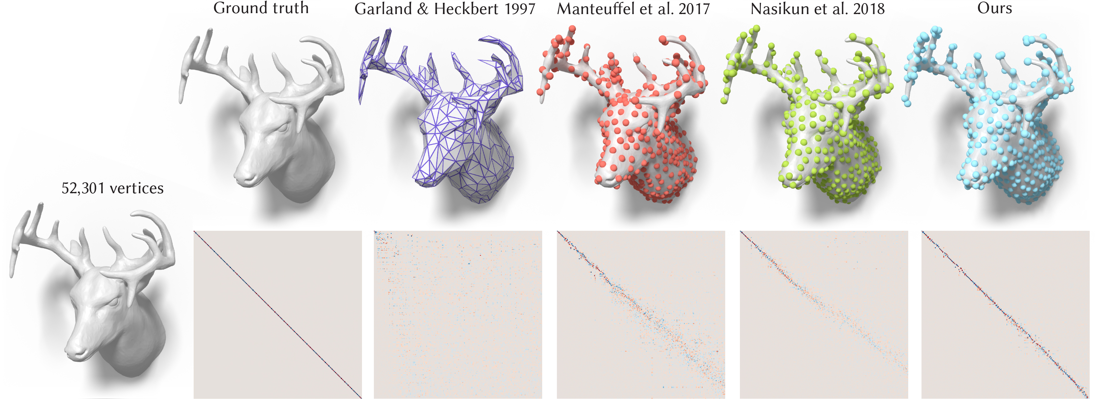
Figure 1. There are many ways to coarsen a 52,301$×$52,301 sparse anisotropic Laplace matrix down to a sparse 500$×$500 matrix: simplify the mesh [Garland and Heckbert, 1997] and rediscretize; apply algebraic multigrid coarsening [Manteuffel et al., 2017]; or approximate using radial-basis functions [Nasikun et al., 2018]. We introduce a way to measure how well the coarse operator maintains the original operator’s eigenvectors (bottom row). The visualization shows deviation from a diagonal matrix indicating poor eigenvector preservation. In response, we introduce an optimization to coarsen geometric operators while preserving eigenvectors and maintaining sparsity and positive semi-definiteness.

1. Introduction

Geometry processing relies heavily on building matrices to represent linear operators defined on geometric domains. While typically sparse, these matrices are often too large to work with efficiently when defined over high resolution representations. A common solution is to simplify or coarsen the domain. However, matrices built from coarse representations often do not behave the same way as their fine counterparts leading to inaccurate results and artifacts when resolution is restored. Quantifying and categorizing how this behavior is different is not straightforward and most often coarsening is achieved through operator-oblivious remeshing. The common appearance-based or geometric metrics employed by remeshers, such as the classical quadratic error metric [Garland and Heckbert, 1997] can have very little correlation to maintaining operator behavior.

We propose a novel way to compare the spectral properties of a discrete operator before and after coarsening, and to guide the coarsening to preserve them. Our method is motivated by the recent success of spectral methods in shape analysis and processing tasks, such as shape comparison and non-rigid shape matching, symmetry detection, and vector field design to name a few. These methods exploit eigenfunctions of various operators, including the Laplace-Beltrami operator, whose eigenfunctions can be seen as a generalization of the Fourier basis to curved surfaces. Thus, spectral methods expand the powerful tools from Fourier analysis to more general domains such as shapes, represented as triangle meshes in 3D. We propose to measure how well the eigenvectors (and by extension eigenvalues) of a matrix $\mathsf{L}∈\mathbb{R}^{n×n}$ on

the high-resolution domain are maintained by its coarsened counterpart $\widetilde{\mathsf{L}}∈\mathbb{R}^{m×m}$ ($m<n$) by computing a dense matrix $\mathsf{C}^{k×k}$, defined as the inner product of the first $k$ eigenvectors $\Phi∈\mathbb{R}^{n×k}$ and $\widetilde{Φ}∈\mathbb{R}^{m×k}$ of $\mathsf{L}$ and $\widetilde{\mathsf{L}}$ respectively:

(1) $$\mathsf{C}=\widetilde{Φ}^{\top}\widetilde{\mathsf{M}}\mathsf{P}\Phi,$$

where $\widetilde{\mathsf{M}}∈\mathbb{R}^{m×m}$ defines a mass-matrix on the coarse domain and $\mathsf{P}∈\mathbb{R}^{m×n}$ is a restriction operator from fine to coarse. The closer $\mathsf{C}$ resembles the identity matrix the more the eigenvectors of the two operators before and after coarsening are equivalent.

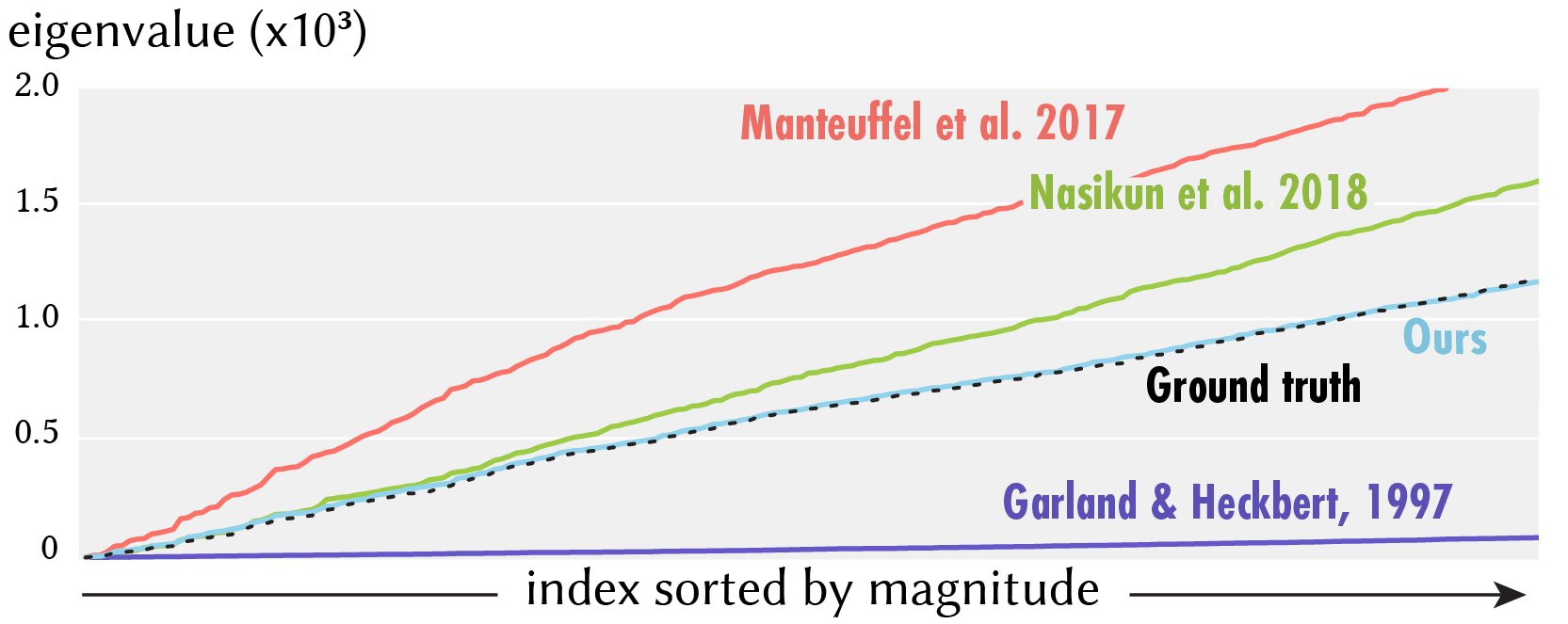
Figure 2. Our coarsening directly preserves eigenvectors so eigenvalues are also implicitly preserved: eigenvalue plot of Fig. 1.

We show through a variety of examples that existing geometric and algebraic coarsening methods fail to varying degrees to preserve the eigenvectors and the eigenvalues of common operators used in geometry processing (see Fig. 1 and Fig. 2).

In response, we propose a novel coarsening method that achieves much better preservation under this new metric. We present an optimization strategy to coarsen an input positive semi-definite matrix in a way that better maintains its eigenvectors (see Fig. 1, right) while preserving matrix sparsity and semi-definiteness. Our optimization is designed for operators occurring in geometry processing and computer graphics, but does not rely on access to a geometric mesh: our input is the matrix $\mathsf{L}$, and an area measure $\mathsf{M}$ on the fine domain, allowing us to deal with non-uniform sampling. The output coarsened operator $\widetilde{\mathsf{L}}$ and an area measure $\widetilde{\mathsf{M}}$ on the coarse domain are defined for a subset of the input elements chosen carefully to respect anisotropy and irregular mass distribution defined by the input operator. The coarsened operator is optimized via a novel formulation of coarsening as a sparse semi-definite programming optimization based on the operator commutative diagram.

We demonstrate the effectiveness of our method at categorizing the failure of existing methods to maintain eigenvectors on a number of different examples of geometric domains including triangle meshes, volumetric tetrahedral meshes and point clouds. In direct comparisons, we show examples of successful spectral coarsening for isotropic and anisotropic operators. Finally, we provide evidence that spectral coarsening can improve downstream applications such as shape matching, graph pooling for graph convolutional neural networks, and data-driven mesh sampling.

2. Related Work

Mesh Simplification and Hierarchical Representation

The use of multi-resolution shape representations based on mesh simplification has been extensively studied in computer graphics, with most prominent early examples including mesh decimation and optimization approaches [Schroeder et al., 1992; Hoppe et al., 1993] and their multiresolution variants e.g., progressive meshes [Hoppe, 1996; Popović and Hoppe, 1997] (see [Cignoni et al., 1998] for an overview and comparison of a wide range of mesh simplification methods). Among these classical techniques, perhaps the best-known and most widely used approach is based on the quadratic error metrics introduced in [Garland and Heckbert, 1997] and extended significantly in follow-up works e.g., to incorporate texture and appearance attributes [Garland and Heckbert, 1998; Hoppe, 1999] to name a few. Other, more recent approaches have also included variational shape approximation [Cohen-Steiner et al., 2004] and wavelet-based methods especially prominent in shape compression [Schroder, 1996; Peyré and Mallat, 2005], as well as more flexible multi-resolution approaches such as those based on hybrid meshes [Guskov et al., 2002] among myriad others. Although mesh simplification is a very well-studied problem, the vast majority of approximation techniques is geared towards preservation of shape appearance most often formulated via the preservation of local geometric features. Li et al. [2015] conduct a frequency-adaptive mesh simplification to better preserve the acoustic transfer of a shape by appending a modal displacement as an extra channel during progressive meshes. In Fig. 3, we show that this method fails to preserve all low frequency eigenvectors (since it is designed for a single frequency). Our measure helps to reveal the accuracy of preserving spectral quantities, and to demonstrate that existing techniques often fail to achieve this objective.

Numerical Coarsening in Simulation

Coarsening the geometry of an elasticity simulation mesh without adjusting the material parameters (e.g., Young’s modulus) leads to numerical stiffening. Kharevych et al. [2009] recognize this and propose a method to independently adjust the per-tetrahedron elasticity tensor of a coarse mesh to agree with the six smallest deformation modes of a fine-mesh inhomogeneous material object (see Fig. 3 for comparison).

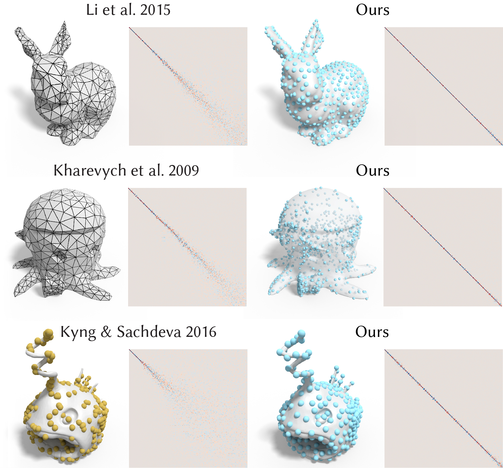
Figure 3. As methods of Li et al. [2015]; Kharevych et al. [2009]; Kyng and Sachdeva [2016] are not designed for preserving spectral properties, they only preserve very low frequency eigenvectors (top-left corner of matrix images), but fails for subsequent modes.

Chen et al. [2015] extend this idea via a data-driven lookup table. Chen et al. [2018] consider numerical coarsening for regular-grid domains, where matrix-valued basis functions on the coarse domain are optimized to again agree with the six smallest deformation modes of a fine mesh through a global quadratic optimization. To better capture vibrations, Chen et al. [2017] coarsen regular-grids of homogeneous materials until their low frequency vibration modes exceeding a Hausdorff distance threshold. The ratio of the first eigenvalue before and after coarsening is then used to rescale the coarse materials Young’s modulus. In contrast to these methods, our proposed optimization is not restricted to regular grids or limited by adjusting physical parameters directly.

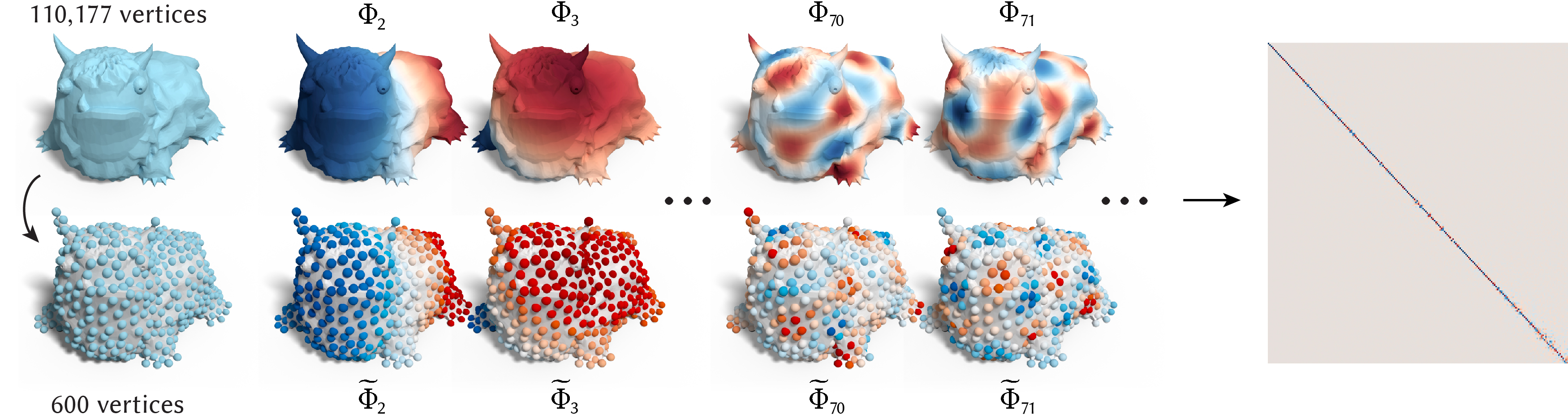
Figure 4. When eigenvectors are equivalent (up to sign) before and after coarsening the operator, the matrix $\mathsf{C}$ (right) resembles the identity matrix.

Algebraic Multigrid

Traditional multigrid methods coarsen the mesh of the geometric domain recursively to create an efficient iterative solver for large linear systems [Briggs et al., 2000]. For isotropic operators, each geometric level smooths away error at the corresponding frequency level [Burt and Adelson, 1983]. Algebraic multigrid (AMG) does not see or store geometric levels, but instead defines a hierarchy of system matrices that attempt to smooth away error according to the input matrix’s spectrum [Xu and Zikatanov, 2017]. AMG has been successfully applied for anisotropic problems such as cloth simulation [Tamstorf et al., 2015]. Without access to underlying geometry, AMG methods treat the input sparse matrix as a graph with edges corresponding to non-zeros and build a coarser graph for each level by removing nodes and adding edges according to an algebraic distance determined by the input matrix. AMG like all multigrid hierarchies are typically measured according to their solver convergence rates [Xu and Zikatanov, 2017]. While eigenvector preservation is beneficial to AMG, an efficient solver must also avoid adding too many new edges during coarsening (i.e., [Livne and Brandt, 2012; Kahl and Rottmann, 2018]). Meanwhile, to remain competitive to other blackbox solvers, AMG methods also strive to achieve very fast hierarchy construction performance [Xu and Zikatanov, 2017]. Our analysis shows how state-of-the-art AMG coarsening methods such as [Manteuffel et al., 2017] which is designed for fast convergence fails to preserve eigenvectors and eigenvalues (see Fig. 1 and Fig. 2). Our subsequent optimization formulation in Section 3.1 and Section 3.2 is inspired by the “root node” selection and Galerkin projection approaches found in the AMG literature [Stuben, 2000; Bell, 2008; Manteuffel et al., 2017].

Spectrum Preservation

In contrast to geometry-based mesh simplification very few methods have been proposed targeting preservation of spectral properties. Öztireli and colleagues [Öztireli et al., 2010] introduced a technique for spectral sampling on surfaces. In a similar spirit to our approach, their method aims to compute samples on a surface that can approximate the Laplacian spectrum of the original shape. This method targets only isotropic sampling and is not well-suited to more diverse operators such as the anisotropic Laplace-Beltrami operator handled by our approach. More fundamentally, our goal is to construct a coarse representation that preserves an entire operator, and allows, for example to compute eigenfunctions and eigenvalues in the coarse domain, which is not addressed by a purely sampling-based strategy. More recently, an efficient approach for approximating the Laplace-Beltrami eigenfunctions has been introduced in [Nasikun et al., 2018], based on a combination of fast Poisson sampling and an adapted coarsening strategy. While very efficient, as we show below, this method unfortunately fails to preserve even medium frequencies, especially in the presence of high-curvature shape features or more diverse, including anisotropic Laplacian, operators.

We note briefly that spectrum preservation and optimization has also been considered in the context of sound synthesis, including [Bharaj et al., 2015], and more algebraically for efficient solutions of Laplacian linear systems [Kyng and Sachdeva, 2016]. In Fig. 3, we show that the method of Kyng and Sachdeva [2016] only preserves very low frequency eigenvectors. Our approach is geared towards operators defined on non-uniform triangle meshes and does not have limitations of the approach of [Kyng and Sachdeva, 2016] which only works on Laplacians where all weights are positive.

3. Method

The input to our method is a $n$-by-$n$ sparse, positive semi-definite matrix $\mathsf{L}∈\mathbb{R}^{n×n}$. We assume $\mathsf{L}$ is the Hessian of an energy derived from a geometric domain with $n$ vertices and the sparsity pattern is determined by the connectivity of a mesh or local neighbor relationship. For example, $\mathsf{L}$ may be the discrete cotangent Laplacian, the Hessian of the discrete Dirichlet energy. However, we do not require direct access to the geometric domain or its spatial embedding. We also take as input a non-negative diagonal weighting or mass matrix $\mathsf{M}∈\mathbb{R}^{n×n}$ (i.e., defining the inner-product space of vectors from the input domain). The main parameter of our method is the positive number $m<n$ which determines the size of our coarsened output.

Our method outputs a sparse, positive semi-definite matrix $\widetilde{\mathsf{L}}∈\mathbb{R}^{m×m}$ that attempts to maintain the low-frequency eigenvalues and eigenvectors of the input matrix $\mathsf{L}$ (see Fig. 4).

$\mathsf{P},\mathsf{K}\textleftarrow\textit{combinatorial coarsening}(\mathsf{L},\mathsf{M},m)$;

$\widetilde{\mathsf{L}},\widetilde{\mathsf{M}}\textleftarrow\textit{operator optimization}(\mathsf{L},\mathsf{M},\mathsf{P},\mathsf{K})$;

Algorithm 1 Spectral Coarsening given $\mathsf{L}$, $\mathsf{M}$ and $m$

We propose coarsening in two steps (see Algorithm 1). First we treat the input matrix $\mathsf{L}$ as encoding a graph and select a subset of $m$ “root” nodes, assigning all others to clusters based on a novel graph-distance. This clustering step defines a restriction operator ($\mathsf{P}$ in Eq. 1) and a cluster-assignment operator $\mathsf{K}$ that determines the sparsity pattern of our output matrix $\widetilde{\mathsf{L}}$. In the second stage, we optimize the non-zero values of $\widetilde{\mathsf{L}}$.

3.1. Combinatorial coarsening

Given an input operator $\mathsf{L}∈\mathbb{R}^{n×n}$ and corresponding mass-matrix $\mathsf{M}∈\mathbb{R}^{n×n}$, the goal of this stage is to construct two sparse binary matrices $\mathsf{K},\mathsf{P}∈\{0,1\}^{m×n}$ (see Fig. 5). Acting as a cluster-assignment operator, $\mathsf{K}$ has exactly one $1$ per column, so that $\mathsf{K}_{ij}=1$ indicates that element $j$ on the input domain is assigned to element $i$ on the coarsened domain. Complementarily, acting as a restriction or subset-selection operator, $\mathsf{P}$ has exactly one $1$ per row and

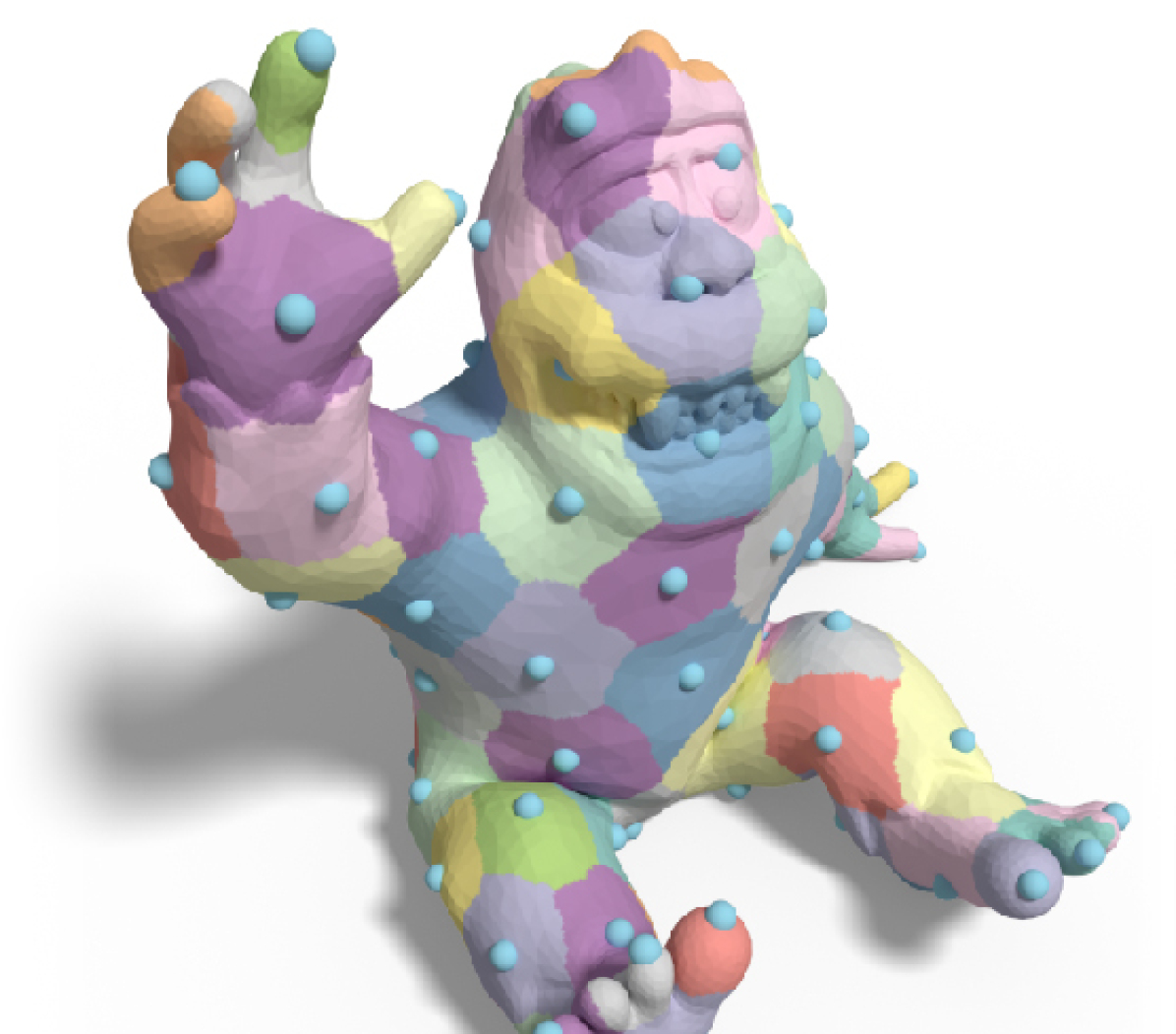
Figure 5. Blue dots and colored regions indicate “root nodes” and clusters selected by $\mathsf{P}$ and $\mathsf{K}$ respectively.

no more than one $1$ per column, so that $\mathsf{P}_{ij}=1$ indicates that element $j$ on the input domain is selected as element $i$ in the coarsened domain to represent its corresponding cluster. Following the terminology from the algebraic multigrid literature, we refer to this selected element as the “root node” of the cluster [Manteuffel et al., 2017]. In our figures, we visualize $\mathsf{P}$ by drawing large dots on the selected nodes and $\mathsf{K}$ by different color segments.

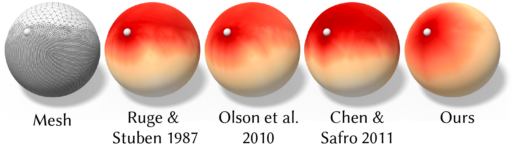
Figure 6. We visualize the graph shortest path distance from the source point (gray) to all the other points, where the strength of connections between adjacent points is defined using different operator-dependent strength measures. In an isotropic problem, our resulting “distance” is more robust to different element sizes and grows more uniformly in all directions (right).

Consider the graph with $n$ nodes implied by interpreting non-zeros of $\mathsf{L}$ as undirected edges. Our node-clustering and root-node selection should respect how quickly information at one node diffuses to neighboring nodes according to $\mathsf{L}$ and how much mass or weight is associated with each node according to $\mathsf{M}$. Although a variety of algebraic distances have been proposed [Ruge and Stüben, 1987; Chen and Safro, 2011; Olson et al., 2010; Livne and Brandt, 2012], they are not directly applicable to our geometric tasks because they are sensitive to different finite-element sizes (see Fig. 6).

According to this diffusion perspective, the edge-distance of the edge between nodes $i$ and $j$ should be inversely correlated with $-\mathsf{L}_{ij}$ and positively correlated with $(\mathsf{M}_{ii}+\mathsf{M}_{jj})$. Given the units of $\mathsf{L}$ and $\mathsf{M}$ in terms of powers of length $p$ and $q$ respectively (e.g., the discrete cotangent Laplacian for a triangle mesh has units $p$=0, the barycentric mass matrix has units $q$=2), then we adjust these correlations so that our edge-distance has units of length. Putting these relations together and avoiding negative lengths due to positive off-diagonal entries in $\mathsf{L}$, we define the edge-distance between connected nodes as:

$$\mathsf{D}_{ij}=\max\left(\frac{(\mathsf{M}_{ii}+\mathsf{M}_{jj})^{(p+1)/q}}{-\mathsf{L}_{ij}},0\right).$$

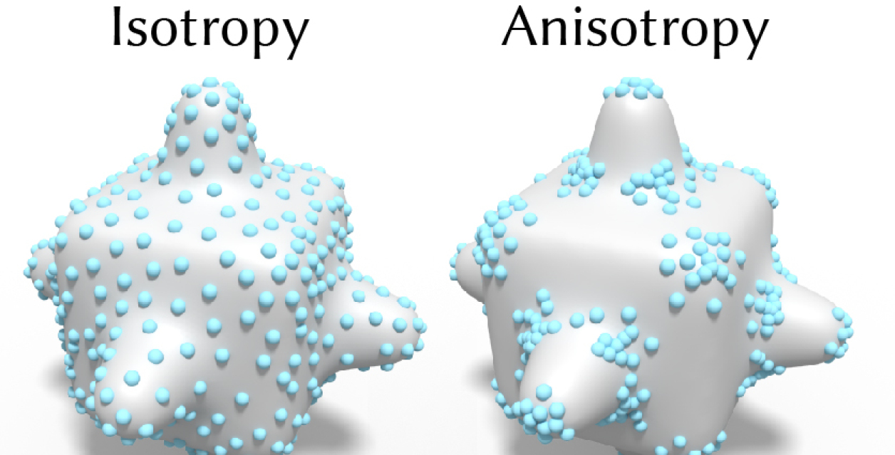
Figure 7. Our coarsening is aware of the anisotropy of the underlying operator, resulting in a different set of selected root nodes.

Compared to Euclidean or geodesic distance, shortest-path distances using this edge-distance will respect anisotropy of $\mathsf{L}$ (see Fig. 7, Fig. 8). Compared to state-of-the-art algebraic distances, our distance will account for irregular mass distribution, e.g., due to irregular meshing (see Fig. 6).

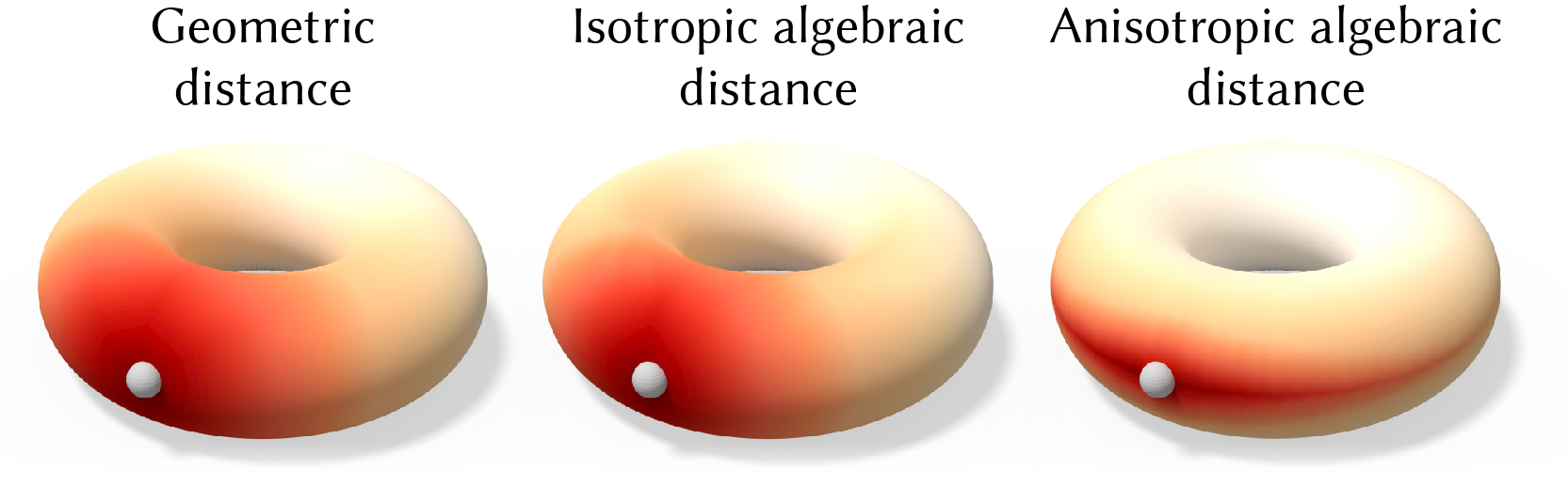
Figure 8. We visualize the graph shortest path distance from the source point (gray) to all the other points. Our operator-dependent distance can handle both isotropic and anisotropic problems, whereas standard geometry-based measure (e.g. edge length) is limited to isotropic problems.

Given this (symmetric) matrix of edge-distances, we compute the $k$-mediods clustering [Struyf et al., 1997] of the graph nodes according to shortest path distances (computed efficiently using the modified Bellman-Ford method and Lloyd aggregation method of Bell [2008]). We initialize this iterative optimization with a random set of $k$ root nodes. Unlike $k$-means where the mean of each cluster is not restricted to the set of input points in space, $k$-mediods chooses the cluster root as the mediod-node of the cluster (i.e., the node with minimal total distance to all other nodes in the cluster). All other nodes are then re-assigned to their closest root. This process is iterated until convergence. Cluster assignments and cluster roots are stored as $\mathsf{K}$ and $\mathsf{P}$ accordingly. Comparing to the farthest point sampling and the random sampling, our approach results in a better eigenfunction preservation image for anisotropic operators (Fig. 9).

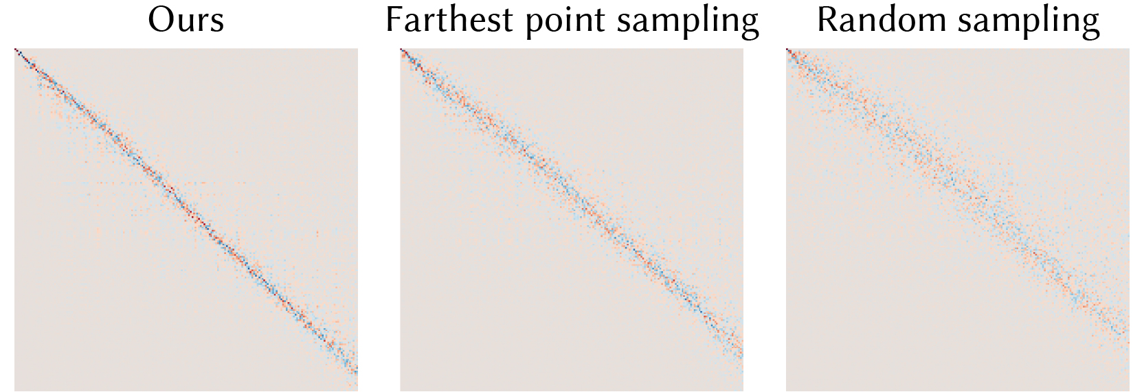
Figure 9. Coarsening with our operator-aware distance (left) results in a better eigenfunction preservation compared to the farthest point sampling (middle) and the random sampling (right) on an anisotropic operator.

We construct a sparsity pattern for $\widetilde{\mathsf{L}}$ so that $\widetilde{\mathsf{L}}_{ij}$ may be non-zero if the cluster $j$ is in the three-ring neighborhood of cluster $i$ as determined by cluster-cluster adjacency. If we let ${\mathsf{S}_{\mathsf{L}}}∈\{0,1\}^{n×n}$ be a binary matrix containing a 1 if and only if the corresponding element of $\mathsf{L}$ is non-zero, then we can compute the “cluster adjacency” matrix ${\widetilde{\mathsf{A}}}=\mathsf{K}{\mathsf{S}_{\mathsf{L}}}\mathsf{K}^{⊤}∈\{0,1\}^{m×m}$ so that ${\widetilde{\mathsf{A}}}_{ij}=1$ if and only if the clusters $i$ and $j$ contain some elements $u$ and $v$ such that $\mathsf{L}_{uv}≠0$. Using this adjacency matrix, we create a sparse restriction matrix with wider connectivity ${\mathsf{S}_{\mathsf{G}}}=\mathsf{K}^{⊤}{\widetilde{\mathsf{A}}}∈\{0,1\}^{n×m}$. Finally, our predetermined sparsity pattern for $\widetilde{\mathsf{L}}$ is defined to be that of ${\mathsf{S}_{\widetilde{\mathsf{L}}}}={\mathsf{S}_{\mathsf{G}}}^{\top}{\mathsf{S}_{\mathsf{L}}}{\mathsf{S}_{\mathsf{G}}}={\widetilde{\mathsf{A}}}³∈\{0,1\}^{m×m}$. We found that using the cluster three-ring sparsity is a reasonable trade-off between in-fill density and performance of the optimized operator. Assuming the cluster graph is 2-manifold with average valence 6, the three-ring sparsity implies that $\widetilde{\mathsf{L}}$ will have 37 non-zeros per row/column on average, independent to $m$ and $n$. In practice, our cluster graph is nearly 2-manifold. The $\widetilde{\mathsf{L}}$ in Fig. 5, for instance, has approximately $39$ non-zeros per row/column.

3.2. Operator optimization

Given a clustering, root node selection and the desired sparsity pattern, our second step is to compute a coarsened matrix $\widetilde{\mathsf{L}}$ that maintains the eigenvectors of the input matrix $\mathsf{L}$ as much as possible. Since $\mathsf{L}$ and $\widetilde{\mathsf{L}}$ are of different sizes, their corresponding eigenvectors are also of different lengths. To compare them in a meaningful way we will use the functional map matrix $\mathsf{C}$ defined in Eq. 1 implied by the restriction operator $\mathsf{P}$ (note that: prolongation from coarse to fine is generally ill-defined). This also requires a mass-matrix on the coarsened domain, which we compute by lumping cluster masses: $\widetilde{\mathsf{M}}=\mathsf{K}\mathsf{M}\mathsf{K}^{⊤}$. The first $k$ eigenvectors for the input operator and yet-unknown coarsened operator may be computed as solutions to the generalized eigenvalue problems $\mathsf{L}\Phi=Λ\mathsf{M}\Phi$ and $\widetilde{\mathsf{L}}\widetilde{Φ}=\widetilde{Λ}\widetilde{\mathsf{M}}\widetilde{Φ}$, where $Λ,\widetilde{Λ}$ are eigenvalue matrices.

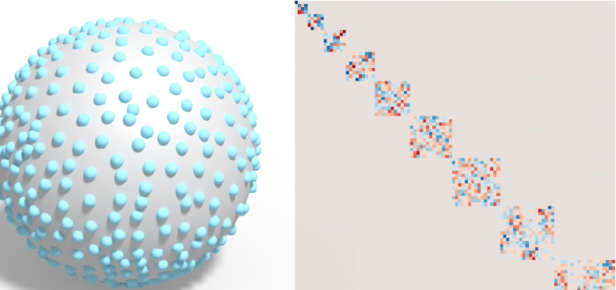
Figure 10. The optimized $\mathsf{C}$ should be block diagonal when the operator has algebraic multiplicity.

Knowing that the proximity of the functional map matrix $\mathsf{C}$ to an identity matrix encodes eigenvector preservation, it might be tempting to try to enforce $\|\mathsf{C}-\mathsf{I}\|_{F}$ directly. This however is problematic because it does not handle sign flips or multiplicity (see Fig. 10). More importantly, recall that in our setting $\mathsf{C}$ is not a free variable, but rather a non-linear function (via eigen decomposition) of the unknown sparse matrix $\widetilde{\mathsf{L}}$.

Instead, we propose to minimize the failure to realize the commutative diagram of a functional map. Ideally, for any function on the input domain $\mathbf{f}∈\mathbb{R}^{n}$ applying the input operator $\mathsf{M}^{-1}\mathsf{L}$ and then the restriction matrix $\mathsf{P}$ is equivalent to applying $\mathsf{P}$ then $\widetilde{\mathsf{M}}^{-1}\widetilde{\mathsf{L}}$, resulting in the same function $\widetilde{\mathbf{f}}∈\mathbb{R}^{m}$ on the coarsened domain:

(7) $$\begin{array}[]{rclcccc}&\mathsf{M}^{-1}\mathsf{L}&\\ {\mathbf{f}}&\xrightarrow{\hskip 34.14322pt}&{\hskip 1.00006pt\bullet\vspace{0.15cm}}\\ \mathsf{P}\left\textdownarrow\vphantom{\int}\right.&&\left\textdownarrow\vphantom{\int}\right.\mathsf{P}\vspace{0.15cm}\\ {\bullet}&\xrightarrow{\hskip 34.14322pt}&\widetilde{\hskip 1.00006pt\mathbf{f}}\\ &\widetilde{\mathsf{M}}^{-1}\widetilde{\mathsf{L}}\end{array}$$

This leads to a straightforward energy that minimizes the difference between the two paths in the commutative diagram for all possible functions $\mathbf{f}$:

(8) $$E(\widetilde{\mathsf{L}})=\|\mathsf{P}\mathsf{M}^{-1}\mathsf{L}\mathsf{I}-\widetilde{\mathsf{M}}^{-1}\widetilde{\mathsf{L}}\mathsf{P}\mathsf{I}\|^{2}_{\widetilde{\mathsf{M}}},$$

where $\mathsf{I}∈\mathbb{R}^{n×n}$ is the identity matrix (included didactically for the discussion that follows) and

$$\|\mathsf{X}\|^{2}_{\widetilde{\mathsf{M}}}=\mathop{\text{tr}}(\mathsf{X}^{⊤}\widetilde{\mathsf{M}}\mathsf{X})$$

computes the Frobenius inner-product defined by $\widetilde{\mathsf{M}}$.

By using $\mathsf{I}$ as the spanning matrix, we treat all functions equally in an L2 sense. Inspired by the functional maps literature, we can instead compute this energy over only lower frequency functions spanned by the first $k$ eigenvectors $\Phi∈\mathbb{R}^{n×k}$ of the operator $\mathsf{L}$. Since high frequency functions naturally cannot live on a coarsened

domain, this parameter $k$ allows the optimization to focus on functions that matter. Consequently, preservation of low frequency eigenvectors dramatically improves (see inset).

Substituting $\Phi$ for $\mathsf{I}$ in Eq. 8, we now consider minimizing this reduced energy $E_{k}$ over all possible sparse positive semi-definite (PSD) matrices $\widetilde{\mathsf{L}}$:

(9) $$\mathop{\text{minimize}}_{\widetilde{\mathsf{L}}≐{\mathsf{S}_{\widetilde{\mathsf{L}}}}}\ \underbrace{\frac{1}{2}\|\mathsf{P}\mathsf{M}^{-1}\mathsf{L}\Phi-\widetilde{\mathsf{M}}^{-1}\widetilde{\mathsf{L}}\mathsf{P}\Phi\|^{2}_{\widetilde{\mathsf{M}}}}_{E_{k}(\widetilde{\mathsf{L}})}$$

(10) subject to $$\ \widetilde{\mathsf{L}}\text{ is positive semi-definite}$$

(11) and $$\ \widetilde{\mathsf{L}}\mathsf{P}\Phi_{0}=0$$

where we use $\mathsf{X}≐\mathsf{Y}$ to denote that $\mathsf{X}$ has the same sparsity pattern as $\mathsf{Y}$. The final linear-equality constraint in Eq. 11 ensures that the eigen-vectors $\Phi_{0}$ corresponding to zero eigenvalues are exactly preserved ($\mathsf{P}\mathsf{L}\Phi_{0}=\mathsf{P}\mathsf{M}\Phi_{0}0=0$). Note that while it might seem that Eq. 9 is only meant to preserve the eigenvectors, a straightforward calculation (See Appendix C) shows that it promotes the preservation of eigenvalues as well.

This optimization problem is convex [Boyd and Vandenberghe, 2004], but the sparsity constraint makes it challenging to solve efficiently. Most efficient semi-definite programming (SDP) solvers (e.g., Mosek, cvxopt, Gurobi) only implement dense PSD constraints. The academic community has studied SDPs over sparse matrices, yet solutions are not immediately applicable (e.g., those based on chordal sparsity [Vandenberghe and Andersen, 2015; Zheng et al., 2017]) or practically efficient (e.g., [Andersen et al., 2010]). Even projecting a sparse matrix $\mathsf{X}$ on to the set of PSD matrices with the same sparsity pattern is a difficult sub-problem (the so-called sparse matrix nearness problem, e.g., [Sun and Vandenberghe, 2015]), so that proximal methods such as ADMM lose their attractiveness.

If we drop the PSD constraint, the result is a simple quadratic optimization with linear constraints and can be solved directly. While this produces solutions with very low objective values $E_{k}$, the eigenvector preservation is sporadic and negative eigenvalues appear (see Fig. 11).

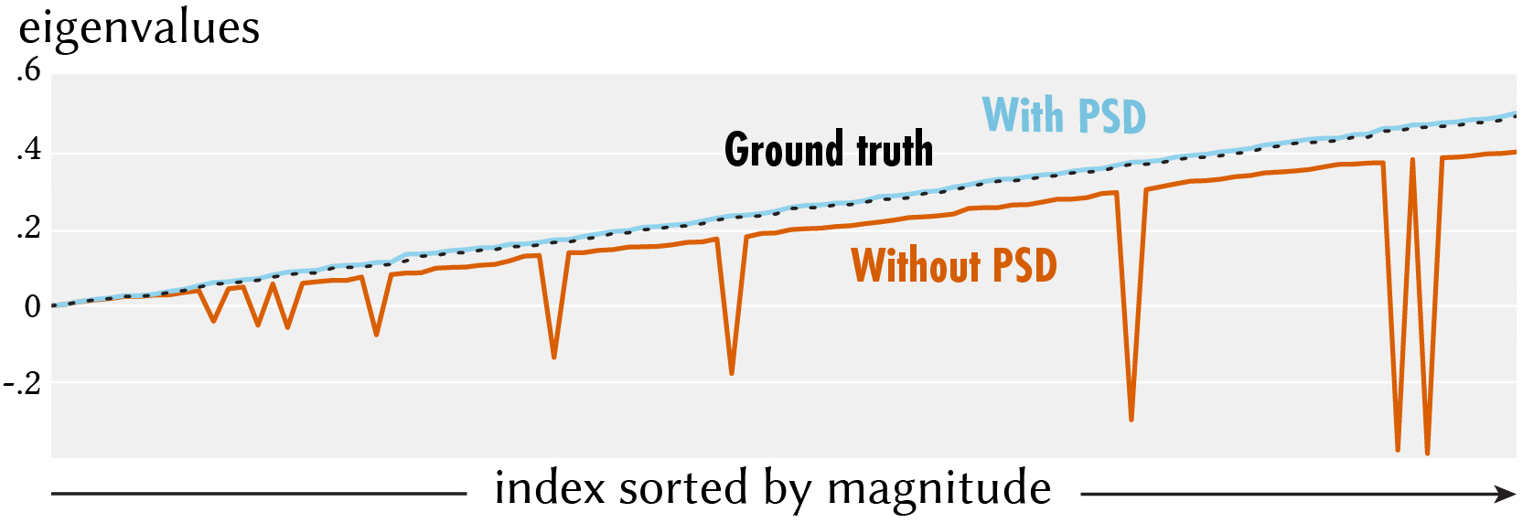
Figure 11. Dropping the PSD constraint leads to a simple quadratic optimization problem which can be solved directly, but it produces a non-PSD $\widetilde{\mathsf{L}}$ that contains negative eigenvalues.

Conversely, attempting to replace the PSD constraint with the stricter but more amenable diagonal dominance linear inequality constraint (i.e., $\widetilde{\mathsf{L}}_{ii}≥∑_{j≠i}\widetilde{\mathsf{L}}_{ji}$) produces a worse objective value and poor eigenvector preservation.

Instead, we propose introducing an auxiliary sparse matrix variable $\mathsf{G}∈\mathbb{R}^{n×m}$ and restricting the coarsened operator to be created by using $\mathsf{G}$ as an interpolation operator: $\widetilde{\mathsf{L}}:=\mathsf{G}^{⊤}\mathsf{L}\mathsf{G}$. Substituting this into Eq. 9, we optimize

(12) $$\mathop{\text{minimize}}_{\mathsf{G}≐{\mathsf{S}_{\mathsf{G}}}}\ \underbrace{\frac{1}{2}\|\mathsf{P}\mathsf{M}^{-1}\mathsf{L}\Phi-\widetilde{\mathsf{M}}^{-1}\mathsf{G}^{⊤}\mathsf{L}\mathsf{G}\mathsf{P}\Phi\|^{2}_{\widetilde{\mathsf{M}}}}_{E_{k}(\mathsf{G})},$$

subject to $$\ \mathsf{G}\mathsf{P}\Phi_{0}=\Phi_{0}$$

where the sparsity of $\widetilde{\mathsf{L}}$ is maintained by requiring sparsity of $\mathsf{G}$. The null-space constraint remains linear because $\mathsf{G}\mathsf{P}\Phi_{0}=\Phi_{0}⇒\mathsf{G}^{⊤}\mathsf{L}\mathsf{G}\mathsf{P}\Phi_{0}=0$ implies that $\widetilde{\mathsf{L}}$ contains the null-space of $\mathsf{L}$. The converse will not necessarily be true, but is unlikely to happen because this would represent inefficient minimization of the objective. In practice, we never found that spurious null-spaces occurred. While we get to remove the PSD constraint ($\mathsf{L}≽0$ implies $\mathsf{G}^{⊤}\mathsf{L}\mathsf{G}≽0$), the price we have paid is that the energy is no longer quadratic in the unknowns, but quartic.

Therefore in lieu of convex programming, we optimize this energy over the non-zeros of $\mathsf{G}$ using a gradient-based algorithm with a fixed step size $γ$. Specifically, we use nadam [Dozat, 2016] optimizer which is a variant of gradient descent that combines momentum and Nesterov’s acceleration. For completeness, we provide the sparse matrix-valued gradient $∂E_{k}/∂\mathsf{G}$ in Appendix A. The sparse linear equality constraints are handled with the orthogonal projection in Appendix B). We summarize our optimization in pseudocode Algorithm 2. We stop the optimization if it stalls (i.e., does not decrease the objective after 10 iterations) and use a fixed step size $γ=0.02$. This rather straightforward application of a gradient-based optimization to maintaining the commutative diagram in Eq. 7 performs quite well for a variety of domains and operators.

$\mathsf{G}\textleftarrow\mathsf{K}^{⊤}$; // initialization

while not stalled do

       $\nicefrac{{∂E_{k}}}{{∂\mathsf{G}}}\textleftarrow\textit{sparse gradient }(\mathsf{G})$;

       $∆\mathsf{G}\textleftarrow\textsc{nadam}(\nicefrac{{∂E_{k}}}{{∂\mathsf{G}}})$;

       $\mathsf{G}\textleftarrow\mathsf{G}-\gamma\ ∆\mathsf{G}$;

       $\mathsf{G}\textleftarrow\textit{orthogonal projection}\,(\mathsf{G},\Phi_{0})$; // see Appendix B

Algorithm 2 Operator optimization using nadam

4. Evaluation & Validation

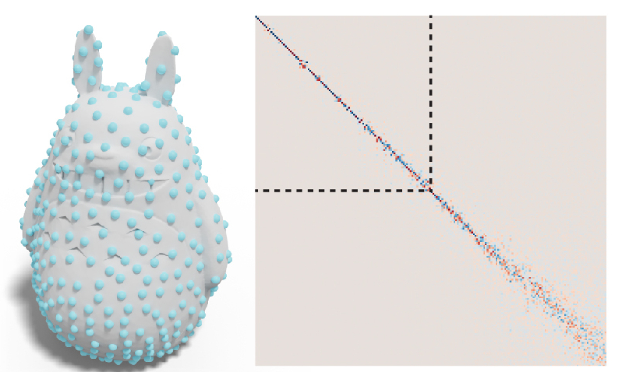
Figure 12. We optimize for the first 100 eigenfunctions and visualize the 200$×$200 functional map, demonstrating a graceful generalization beyond the optimized eigenfunctions.

Our input is a matrix $\mathsf{L}$ which can be derived from a variety of geometric data types. In Fig. 13 we show that our method can preserve the property of the Laplace operators defined on triangle meshes [Pinkall and Polthier, 1993; MacNeal, 1949; Desbrun et al., 1999], point clouds [Belkin et al., 2009], graphs, and tetrahedral meshes [Sharf et al., 2007].

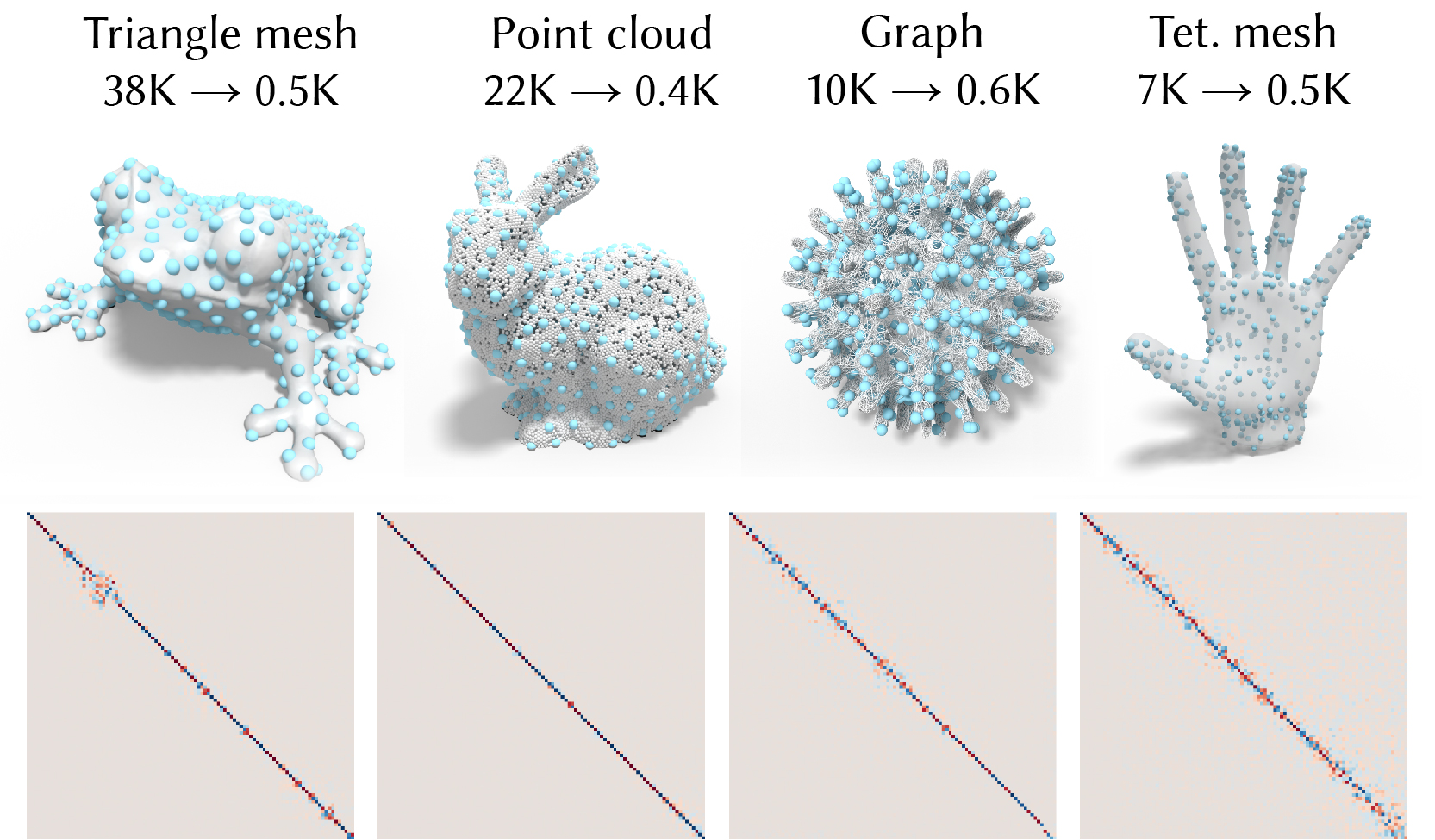
Figure 13. Our algebraic formulation is directly applicable to different data types, such as triangle meshes, point clouds, graphs, and tetrahedral meshes.

We also evaluate our method on a variety of operators, including the offset surface Laplacian [Corman et al., 2017], the Hessian of the Ricci energy [Jin et al., 2008], anisotropic Laplacian [Andreux et al., 2014], and the intrinsic Delaunay Laplacian [Fisher et al., 2006] (see Fig. 14).

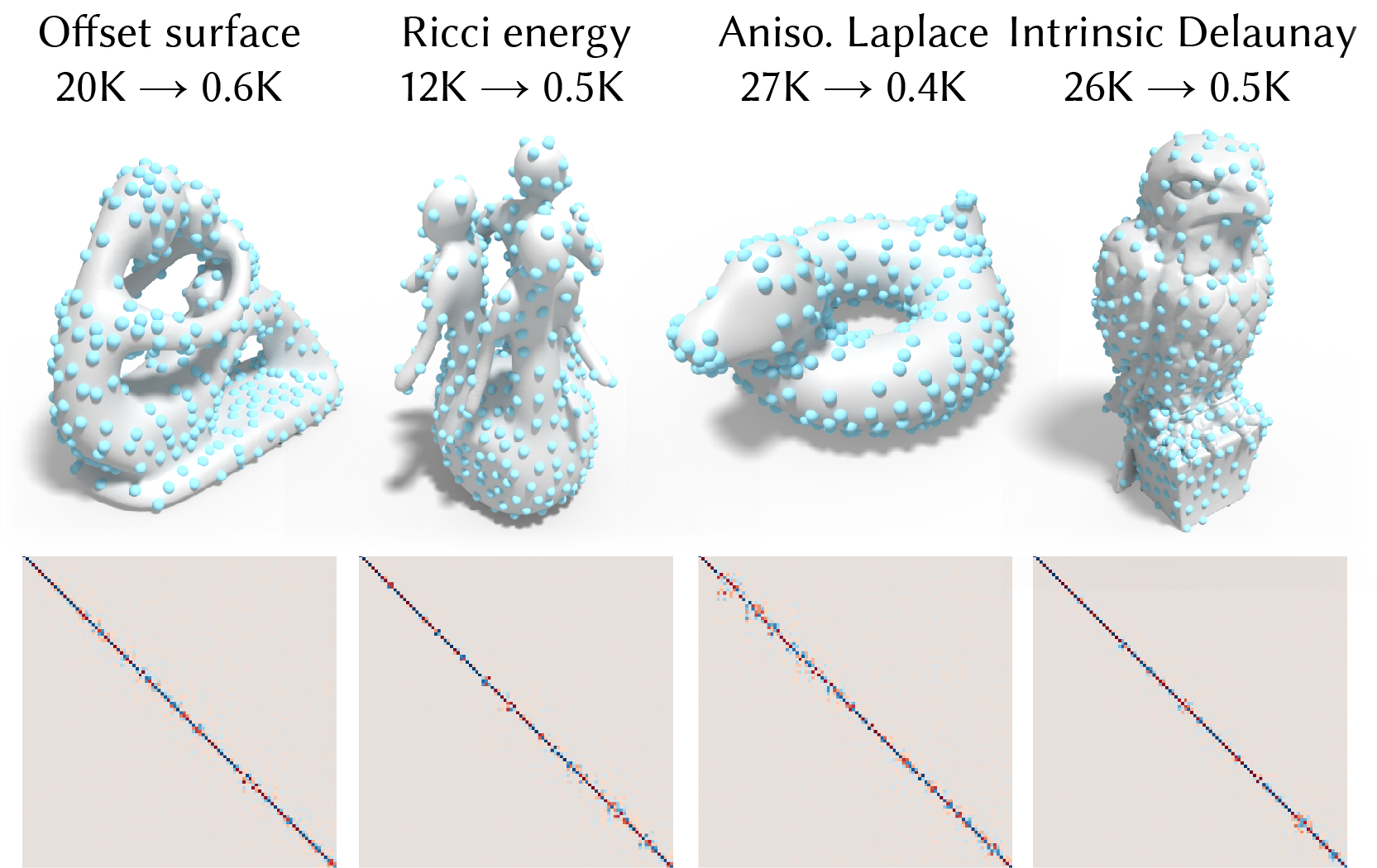
Figure 14. Our method preserves the eigenfunctions of the offset surface Laplacian, the Hessian of the Ricci energy, the anisotropic Laplace, and the the intrinsic Delaunay Laplacian.

We further evaluate how the coarsening generalizes beyond the optimized eigenfunctions. In Fig. 12, we coarsen the shape using the first 100 eigenfunctions and visualize the 200$×$200 functional map image. This shows a strong diagonal for the upper 100$×$100 block and a slowly blurring off-diagonal for the bottom block, demonstrating a graceful generalization beyond the optimized eigenfunctions.

Our algebraic approach takes the operator as the input, instead of the mesh, thus the output quality is robust to noise or sharp features (see Fig. 15). In addition, we can apply our method recursively to the output operator to construct a multilevel hierarchy (see Fig. 16).

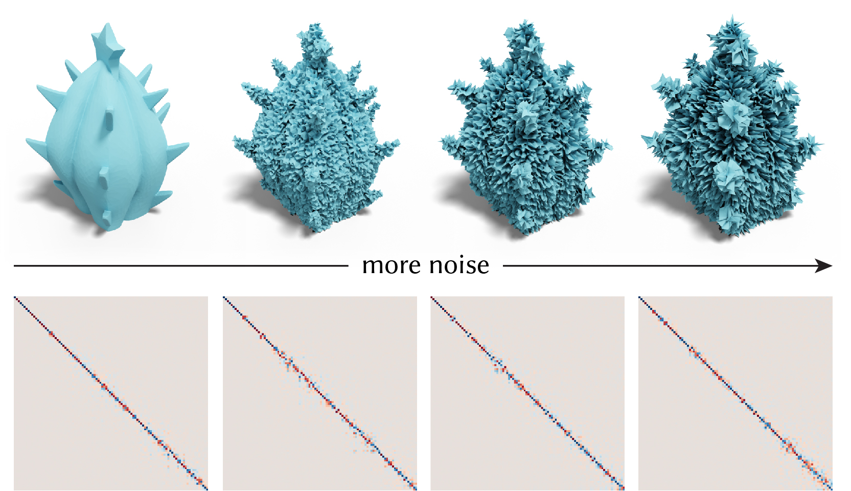
Figure 15. Our coarsening takes the operator as the input, thus the output quality is robust to noise and sharp geometric features.

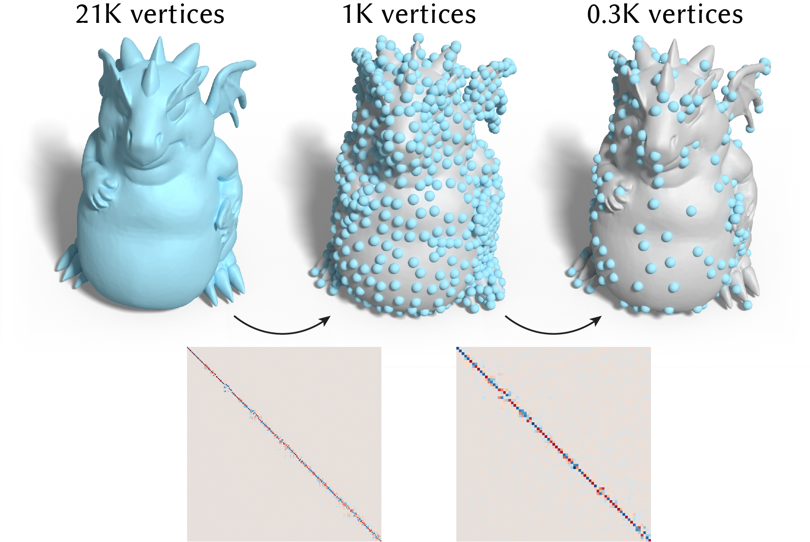
Figure 16. We apply our approach recursively to construct a multilevel hierarchy: from 21,000 rows through 1,000 rows to finally 300 rows.

4.1. Comparisons

Existing coarsening methods are usually not designed for preserving the spectral property of operators. Geometry-based mesh decimation (i.e., QSlim [Garland and Heckbert, 1997]) is formulated to preserve the appearance of the geometry, and results in poor performance in preserving the operator (see Fig. 1). As an iterative solver, algebraic multigrid, i.e., root-node method [Manteuffel et al., 2017], optimizes the convergence rate and does not preserve the spectral properties either. Recently, Nasikun et al. [2018] propose approximating the isotropic Laplacian based on constructing locally supported basis functions. However, this approach falls short in preserving the spectral properties of shapes with high-curvature thin structures and anisotropic operators (see Fig. 17, Fig. 18). In contrast, our proposed method can effectively preserve the eigenfunctions for both isotropic and anisotropic operators.

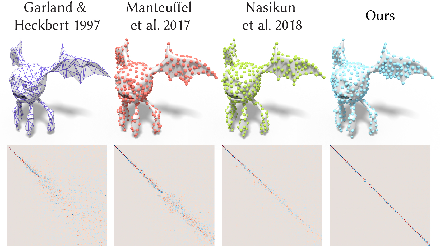
Figure 17. We simplify the cotangent Laplacian from $n=30,000$ to $m=500$. Our coarsening preserve the first 200 eigenfunctions better than the QSlim [Garland and Heckbert, 1997], the root-node algebraic multigrid [Manteuffel et al., 2017], and the fast approximation [Nasikun et al., 2018].

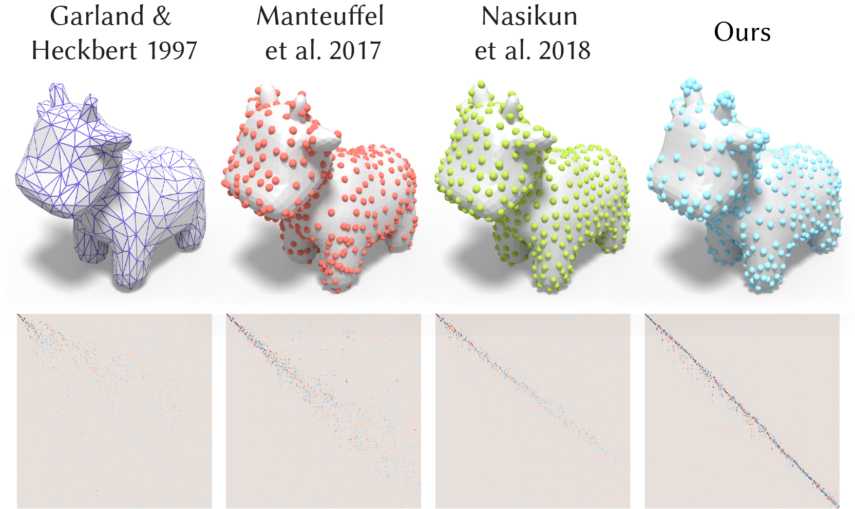
Figure 18. We simplify the anisotropic Laplacian [Andreux et al., 2014] (with parameter 70) from $n=25,000$ to $m=600$. Our approach can preserve eigenfunctions of anisotropic operators better than the existing approaches.

In addition, a simple derivation (Appendix C) can show that minimizing the proposed energy implies eigenvalue preservation (see Fig. 2 and Fig. 19).

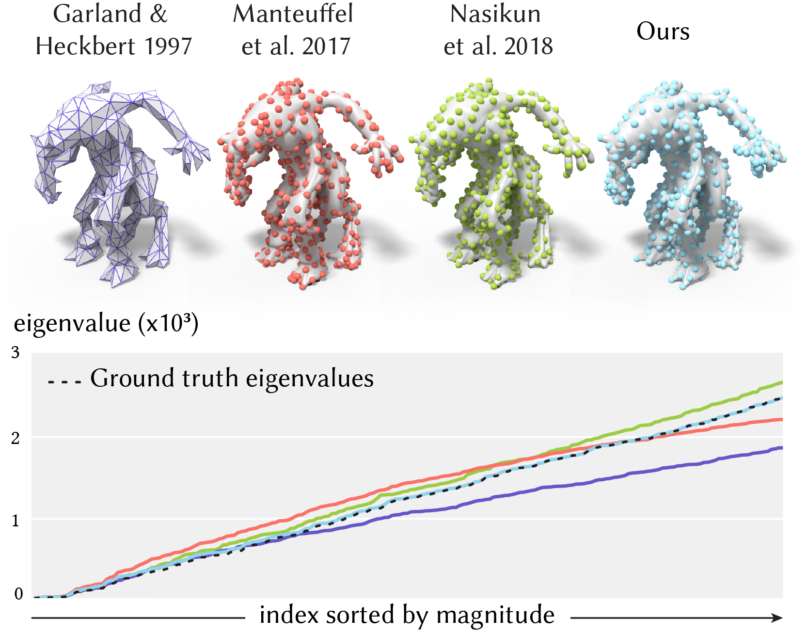
Figure 19. We compare the performance of preserving eigenvalues with different simplification methods. As optimizing our proposed energy implies eigenvalue preservation, we show that the eigenvalues of the simplified operator is well-aligned with the original eigenvalues.

In Fig. 20, we show that our method handles anisotropy in the input operator better than existing methods. This example also demonstrates how our method gracefully degrades as anisotropy increases. Extreme anisotropy (far right column) eventually causes our method to struggle to maintain eigenvectors.

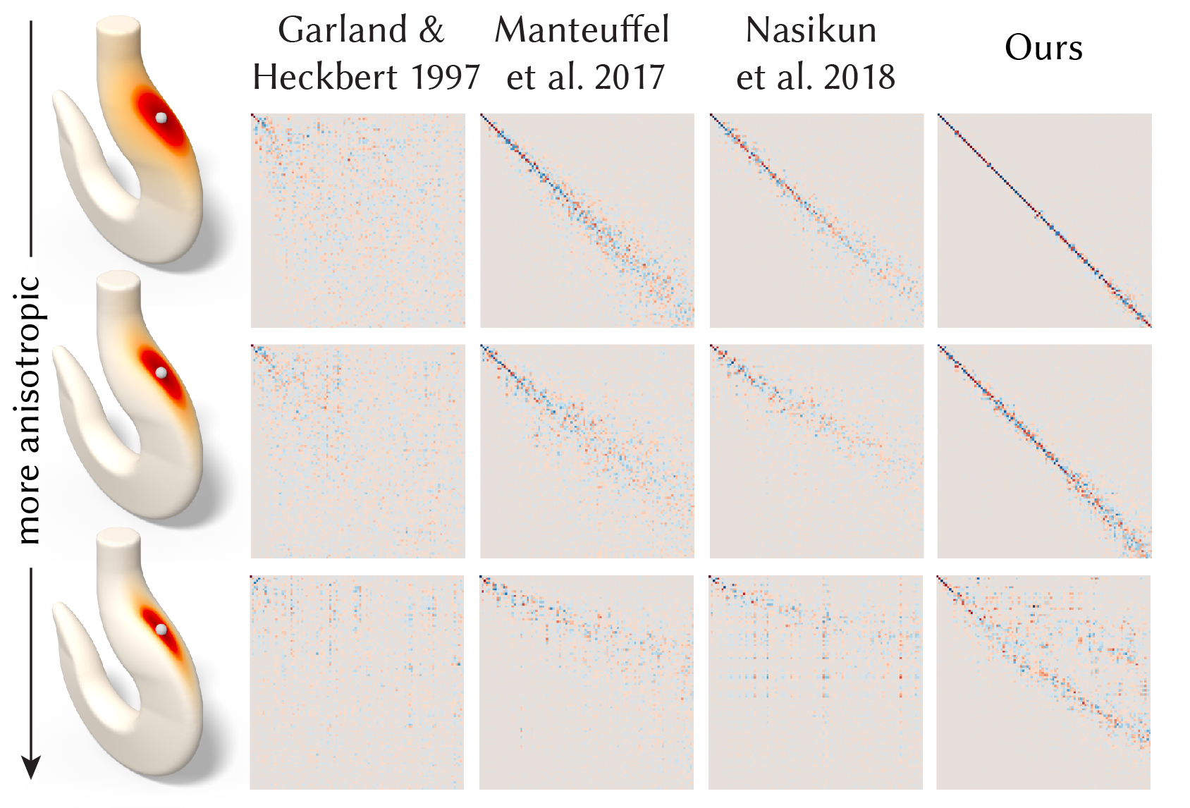
Figure 20. We increase the anisotropy parameter of [Andreux et al., 2014] (60, 120, 180) while simplifying an operator from 21,000 rows down to 500. Our approach handles anisotropy better than existing approaches but still struggles to preserve extreme anisotropic operators.

4.2. Implementation

In general, let $k$ be the number of eigenvectors/eigenvalues in use, we recommend to use the number of root nodes $m>k\times 2$. In Fig. 21 we show that if $m$ is too small, the degrees of freedom are insufficient to capture the eigenfunctions with higher frequencies.

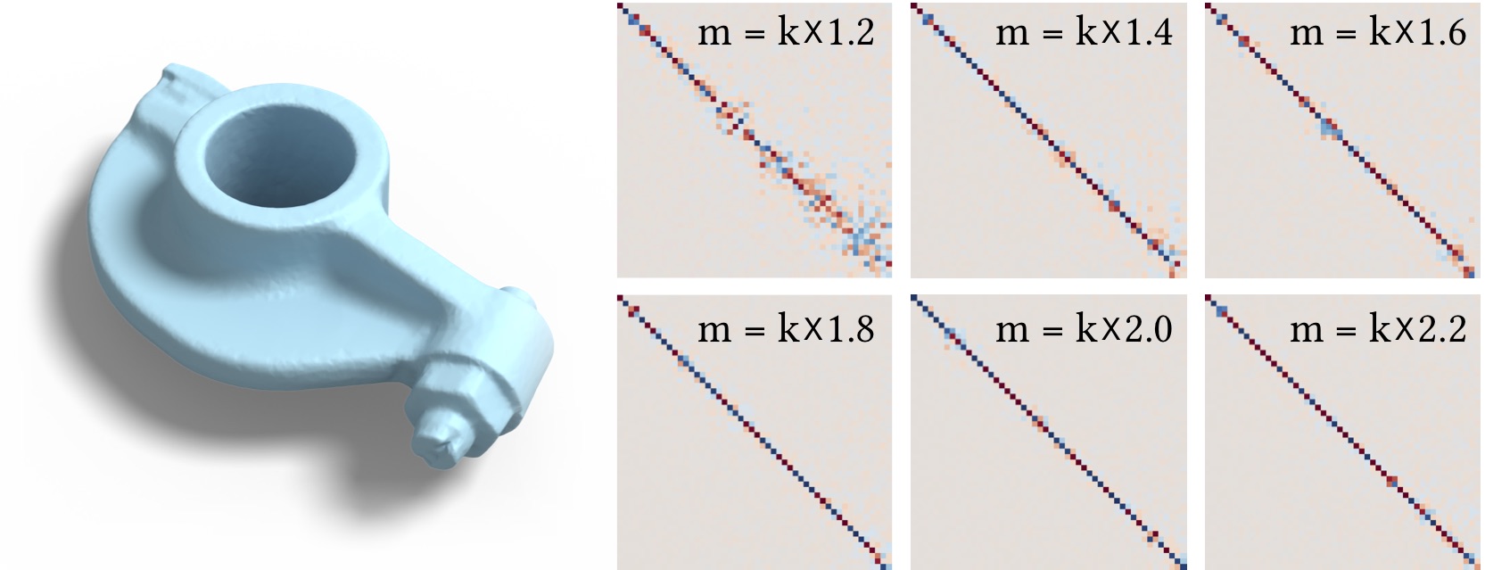
Figure 21. Let $k$ be the number of eigenvectors we want to preserve, experimentally we observed that $m>k\times 2$ leads to desired results.

Our serial C++ implementation is built on top of libigl [Jacobson et al., 2018] and spectra [Qiu, 2018]. We test our implementation on a Linux workstation with an Intel Xeon 3.5GHz CPU, 64GB of RAM, and an NVIDIA GeForce GTX 1080 GPU. We evaluate our runtime using the mesh from Fig. 4 in three different cases: (1) varying the size of input operators $n$, (2) varying the size of output operators $m$, and (3) varying the number of eigenvectors in use $k$. All experiments converge in 100-300 iterations. We report our runtime in Fig. 22. We obtain 3D shapes mainly from Thingi10K [Zhou and Jacobson, 2016] and clean them with the method of [Hu et al., 2018].

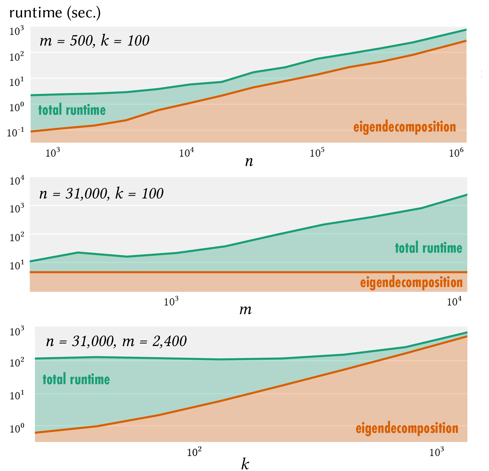
Figure 22. Our runtime shows that our approach is more suitable for aggressive coarsening (middle). For large input meshes and many eigenvectors in use (top, bottom), computing eigendecomposition is the bottleneck.

4.3. Difference-Driven Coarsening

We also validate our combinatorial coarsening by applying it to the shape difference operator [Rustamov et al., 2013] which provides an informative representation of how two shapes differ from each other. As a positive definite operator it fits naturally into our framework. Moreover, since the difference is captured via functional maps, it does not require two shapes to have the same triangulation. We therefore take a pair of shapes with a known functional map between them, compute the shape difference operator and apply our combinatorial coarsening, while trying to best preserve this computed operator. Intuitively, we expect the samples to be informed by the shape difference and thus capture the areas of distortion between the shapes (see Appendix D for more detail). As shown in Fig. 23, our coarsening indeed leads to samples in areas where the intrinsic distortion happens, thus validating the ability of our approach to capture and reveal the characteristics of the input operator.

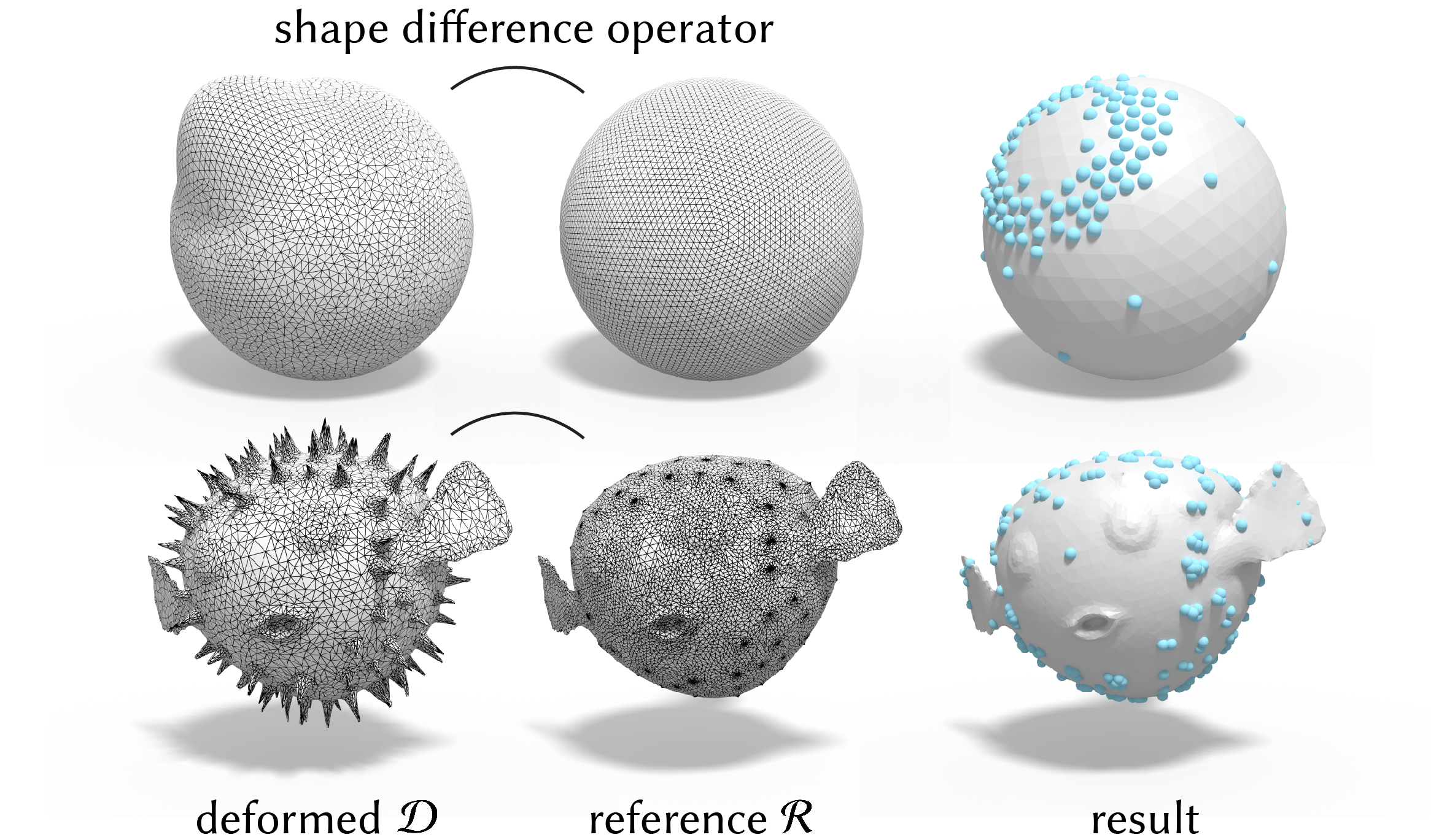
Figure 23. Given a reference shape $\mathcal{R}$ and its deformed version $\mathcal{D}$, we combine the shape difference operator with our coarsening to compute a set of samples that capture the areas of highest distortion between the shapes.

We can further take the element-wise maximum from a collection of shape difference operators to obtain a data-driven coarsening informed by many shape differences (see Fig. 24).

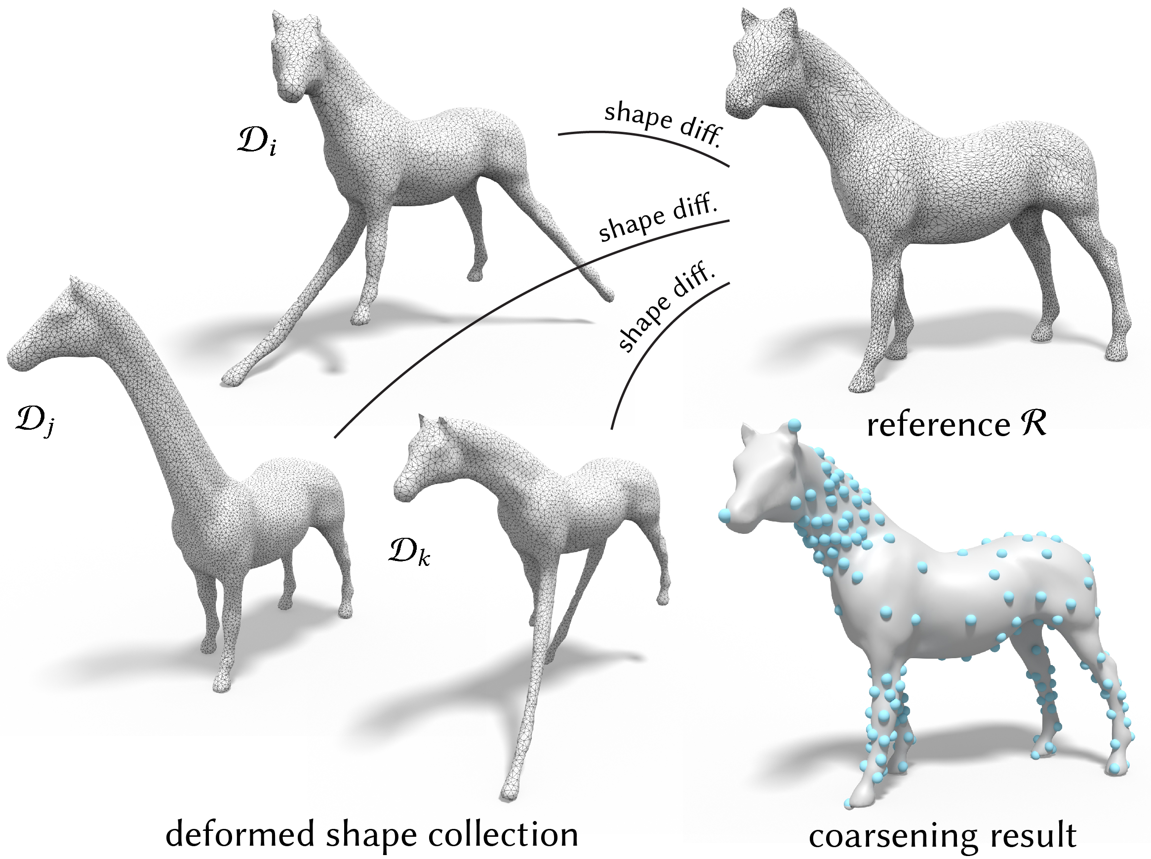
Figure 24. By combining the shape difference operators from the reference shape $\mathcal{R}$ to a collection of deformed shapes $\mathcal{D}$, algebraic coarsening can simplify a mesh based on the “union” of all the deformations.

4.4. Efficient Shape Correspondence

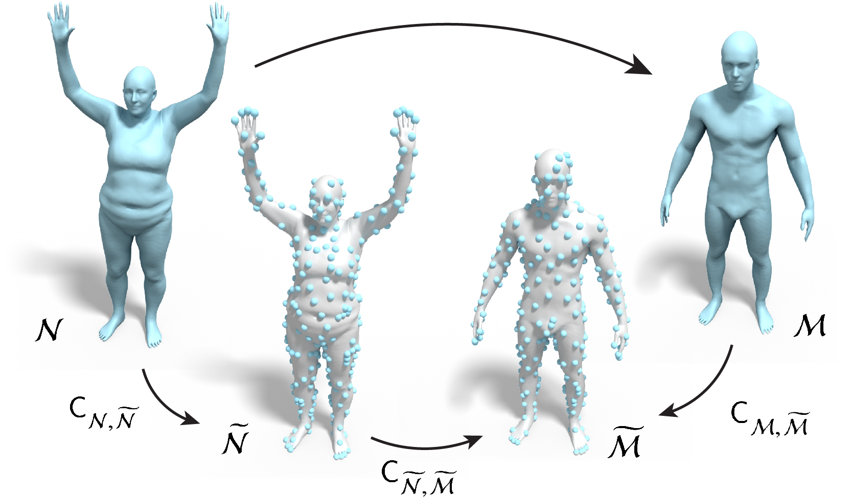
Figure 25. Efficient matching computes the map ${\mathsf{C}_{\mathcal{N},\mathcal{M}}}$ between the original shapes by (1) applying our proposed coarsening to the shape pair and obtain $\mathsf{C}_{\mathcal{N},{\widetilde{\mathcal{N}}}},\mathsf{C}_{\mathcal{M},\widetilde{\mathcal{M}}}$, (2) compute shape correspondences ${\mathsf{C}_{{\widetilde{\mathcal{N}}},\widetilde{\mathcal{M}}}}$ in the reduced space, and (3) solve a linear system based on the commutative diagram.

A key problem in shape analysis is computing correspondences between pairs of non-rigid shapes. In this application we show how our coarsening can significantly speed up existing shape matching methods while also leading to comparable or even higher accuracy. For this we use a recent iterative method based on the notion of Product Manifold Filter (PMF), which has shown excellent results in different shape matching applications [Vestner et al., 2017]. This method, however, suffers from high computational complexity, since it is based on solving a linear assignment problem, $O(n^{3})$, at each iteration. Moreover, it requires the pair of shapes to have the same number of vertices. As a result, in practice before applying PMF shapes are typically subsampled to a coarser resolution and the result is then propagated back to the original meshes. For example in [Litany et al., 2017], the authors used the standard QSlim [Garland and Heckbert, 1997] to simplify the meshes before matching them using PMF. Unfortunately, since standard appearance-based simplification methods can severely distort the spectral properties this can cause problems for spectral methods such as [Vestner et al., 2017] both during matching between coarse domains and while propagating back to the dense ones. Instead our spectral-based coarsening, while not resulting in a mesh provides all the necessary information to apply a spectral technique via the eigen-pairs of the coarse operator, and moreover provides an accurate way to propagate the information back to the original shapes.

More concretely, we aim to find correspondences between the coarsened shapes ${\widetilde{\mathcal{N}}},\widetilde{\mathcal{M}}$ and to propagate the result back to the original domains $\mathcal{N},\mathcal{M}$ by following a commutative diagram (see Fig. 25). When all correspondences are encoded as functional maps this diagam can be written in matrix form as:

(13) $$\mathsf{C}_{\mathcal{M},\widetilde{\mathcal{M}}}\mathsf{C}_{\mathcal{N},\mathcal{M}}=\mathsf{C}_{{\widetilde{\mathcal{N}}},\widetilde{\mathcal{M}}}\mathsf{C}_{\mathcal{N},{\widetilde{\mathcal{N}}}},$$

where $\mathsf{C}_{\mathcal{X},\mathcal{Y}}$ denotes the functional map from $\mathcal{X}$ to $\mathcal{Y}$. Using Eq. 13, the functional map $\mathsf{C}_{\mathcal{N},\mathcal{M}}$ can be computed by solving a simple least squares problem, via a single linear solve. Our main observation is that if the original function space is preserved during the coarsening, less error will be introduced when moving across domains.

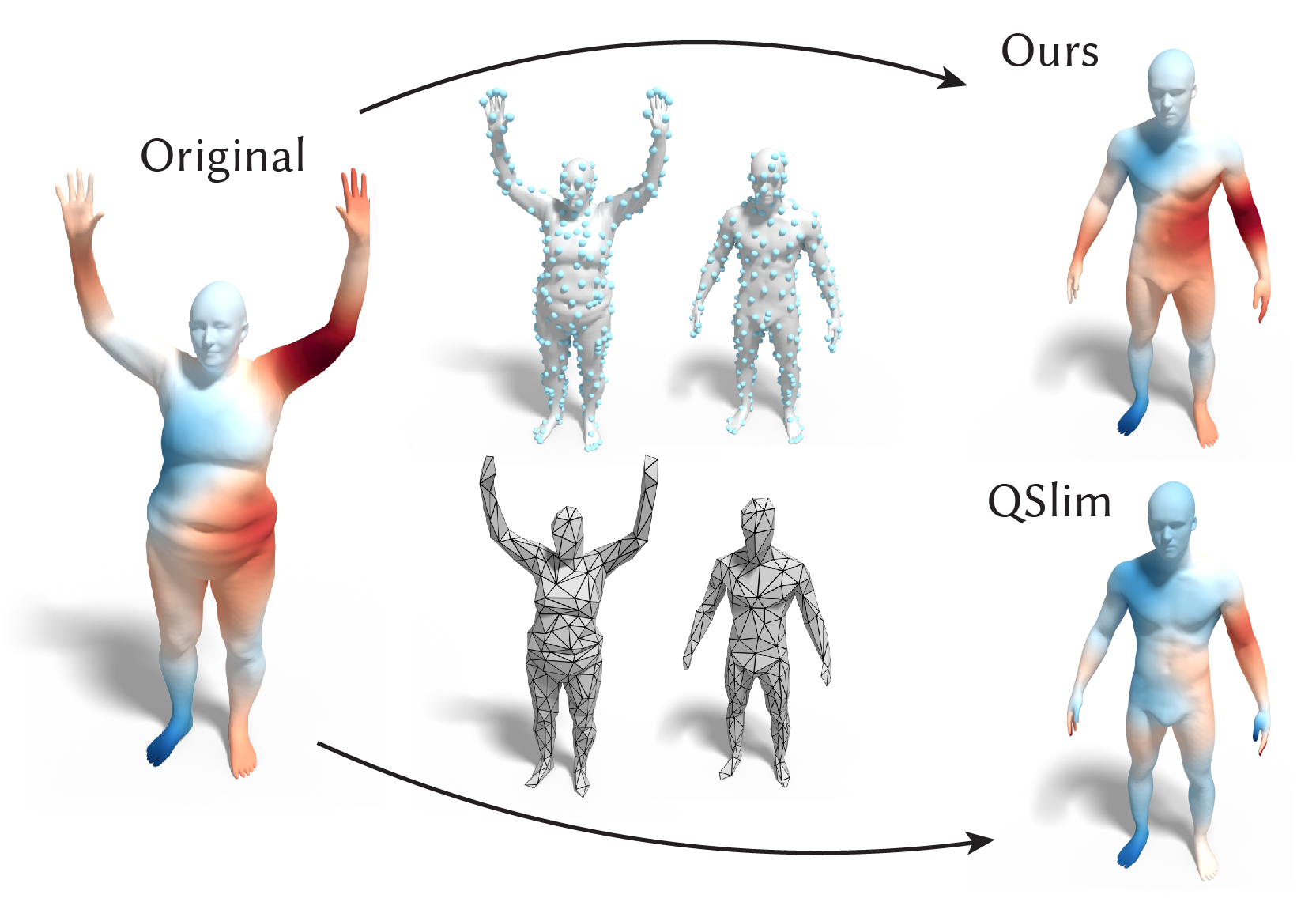
Figure 26. Using our coarsening (top) to infer functional maps between the original pair from the coarse pair introduces less error than using the appearance-based mesh simplification (bottom), QSlim [Garland and Heckbert, 1997].

We tested this approach by evaluating a combination of our coarsening with [Vestner et al., 2017] and compared it to several baselines on a challenging non-rigid non-isometric dataset containing shapes from the SHREC 2007 contest [Giorgi et al., 2007], and evaluated the results using the landmarks and evaluation protocol from [Kim et al., 2011] (please see the details on both the exact parameters and the evaluation in the Appendix). Figure 26 shows the accuracy of several methods, both that directly operate on the dense meshes [Kim et al., 2011; Nogneng and Ovsjanikov, 2017] as well as using kernel matching [Vestner et al., 2017] with QSlim and with our coarsening. The results in Figure 26 show that our approach produces maps with comparable quality or superior quality to existing methods on these non-isometric shape pairs, and results in significant improvement compared to coarsening the shapes with QSlim. At the same time, in Table 1 we report the runtime of different methods, which shows that our approach leads to a significant speed-up compared to existing techniques, and enables an efficient and accurate PMF-based matching method (see Fig. 27) with significantly speedup.

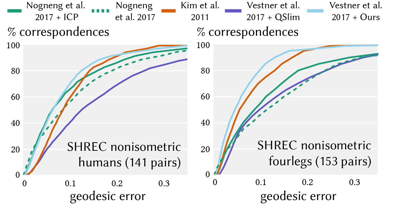
Figure 27. Our efficient shape correspondence with kernel matching [Vestner et al., 2017] achieves comparable matching quality on many non-isometric shape pairs from SHREC [Giorgi et al., 2007] dataset with methods that directly operator on dense meshes [Kim et al., 2011; Nogneng and Ovsjanikov, 2017].

Table 1. We report the total time, pre-computation time + runtime, for computing a 60-by-60 functional map on a shape pair with 14,000 vertices each. Our pre-computation time will be amortized by the number of pairs because we apply coarsening on each shape independently, and the number of combinations is quadratic in the number of shapes. Our runtime is orders of magnitude faster because we only need to perform shape matching in the coarsened domain (i.e., 300 vertices).

[Nogneng 17]+ICP	[Nogneng 17]	[Kim 11]	[Vestner 17]+ours
32.4 $sec$	4.6 $sec$	90.6 $sec$	10.8+0.3 $sec$

4.5. Graph Pooling

Convolutional neural networks [LeCun et al., 1998] have led to breakthroughs in image, video, and sound recognition tasks. The success of CNNs has inspired a growth of interest in generalizing CNNs to graphs and curved surfaces [Bronstein et al., 2017]. The fundamental components of a graph CNN are the pooling and the convolution. Our root node representation $\mathsf{P},\mathsf{K}$ defines a way of performing pooling on graphs. Meanwhile, our output $\widetilde{\mathsf{L}}$ facilitates graph convolution on the coarsened graph due to the convolution theorem [Arfken and Weber, 1999].

To evaluate the performance of graph pooling, we construct several mesh EMNIST datasets where each mesh EMNIST digit is stored as a real-value function on a triangle mesh. Each mesh EMNIST dataset is constructed by overlaying a triangle mesh with the original EMNIST letters [Cohen et al., 2017]. We compare our graph pooling with the graph pooling IN [Defferrard et al., 2016] by evaluating the classification performance. For the sake of fair comparisons, we use the same graph Laplacian, the same architecture, and the smae hyperparameters. The only difference is the graph pooling module. In addition to EMNIST, we evaluate the performance on the fashion-MNIST dataset [Xiao et al., 2017] under the same settings. In Fig. 28, we show that our graph pooling results in better training and testing performance. We provide implementation details in Appendix F.

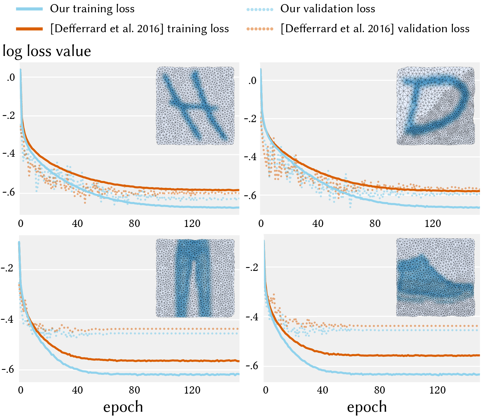
Figure 28. Graph pooling using our coarsening performs better than the pooling presented in [Defferrard et al., 2016] on classifying the mesh EMNIST (top row) and the mesh fashion-MNIST (bottom row) datasets.

5. Limitations & Future Work

Reconstructing a valid mesh from our output coarsened operator would enable more downstream applications. Incorporating a fast eigen-approximation or removing the use of eigen decomposition would further scale the spectral coarsening. Moreover, exploring sparse SDP methods (e.g. [Sun and Vandenberghe, 2015]) could improve our operator optimization. Jointly optimizing the sparsity and the operator entries may lead to even better solutions. Further restricting the sparsity pattern of the coarsened operator while maintaining the performance would aid to the construction of a deeper multilevel representation, which could aid in developing a hierarchical graph representation for graph neural networks. A scalable coarsening with a deeper multilevel representation could promote a multigrid solver for geometry processing applications. Generalizing to quaternions would extend the realm of our coarsening to the fields that deal with quaternionic operators.

6. Acknowledgments

This work is funded in part by by a Google Focused Research Award, KAUST OSR Award (OSR-CRG2017-3426), ERC Starting Grant No. 758800 (EXPROTEA), NSERC Discovery Grants (RGPIN2017-05235), NSERC DAS (RGPAS-2017-507938), the Canada Research Chairs Program, Fields Institute CQAM Labs, Mitacs Globalink, and gifts from Autodesk, Adobe, MESH, and NVIDIA Corporation. We thank members of Dynamic Graphics Project at the University of Toronto and STREAM group at the École Polytechnique for discussions and draft reviews; Eitan Grinspun, Etienne Corman, Jean-Michel Roufosse, Maxime Kirgo, and Silvia Sellán for proofreading; Ahmad Nasikun, Desai Chen, Dingzeyu Li, Gavin Barill, Jing Ren, and Ruqi Huang for sharing implementations and results; Zih-Yin Chen for early discussions.

Appendix A Derivative with Respect to Sparse $\mathsf{G}$

To use a gradient-based solver in Algorithm 2 to solve the optimization problem in Eq. 12 we need derivatives with respect to the non-zeros in $\mathsf{G}$ (the sparsity of ${\mathsf{S}_{\mathsf{G}}}$). We start with the dense gradient:

$$\frac{\partial E_{k}}{\partial\mathsf{G}} =\frac{\partial}{\partial\mathsf{G}}\frac{1}{2}\|\mathsf{P}\mathsf{M}^{-1}\mathsf{L}\Phi-\widetilde{\mathsf{M}}^{-1}\mathsf{G}^{\top}\mathsf{L}\mathsf{G}\mathsf{P}\Phi\|^{2}_{\widetilde{\mathsf{M}}}.$$

We start the derivation by introducing two constant variables $\mathsf{A},\mathsf{B}$ to simplify the expression

$$\frac{\partial E_{k}}{\partial\mathsf{G}}=\frac{\partial}{\partial\mathsf{G}}\frac{1}{2}\|\mathsf{A}-\widetilde{\mathsf{M}}^{-1}\mathsf{G}^{\top}\mathsf{L}\mathsf{G}\mathsf{B}\|^{2}_{\widetilde{\mathsf{M}}}$$

$$\mathsf{A}=\mathsf{P}\mathsf{M}^{-1}\mathsf{L}\Phi,\ \mathsf{B}=\mathsf{P}\Phi.$$

Using the fact that $\mathsf{L},\mathsf{M},\mathsf{M}_{c}$ are symmetric matrices and the rules in matrix trace derivative, we expand the equation as follows.

$$\frac{\partial E_{k}}{\partial\mathsf{G}} =\frac{\partial}{\partial\mathsf{G}}\frac{1}{2}\|\mathsf{A}-\widetilde{\mathsf{M}}^{-1}\mathsf{G}^{\top}\mathsf{L}\mathsf{G}\mathsf{B}\|^{2}_{\widetilde{\mathsf{M}}}$$

$$=\frac{\partial}{\partial\mathsf{G}}\frac{1}{2}\mathop{\text{tr}}\big{(}(\mathsf{A}^{\top}-\mathsf{B}^{\top}\mathsf{G}^{\top}\mathsf{L}\mathsf{G}\widetilde{\mathsf{M}}^{-1})\widetilde{\mathsf{M}}(\mathsf{A}-\widetilde{\mathsf{M}}^{-1}\mathsf{G}^{\top}\mathsf{L}\mathsf{G}\mathsf{B})\big{)}$$

$$=-\frac{\partial}{\partial\mathsf{G}}\Big{(}\mathop{\text{tr}}\big{(}\mathsf{B}^{\top}\mathsf{G}^{\top}\mathsf{L}\mathsf{G}\mathsf{A}\big{)}+\frac{1}{2}\mathop{\text{tr}}\big{(}\mathsf{B}^{\top}\mathsf{G}^{\top}\mathsf{L}\mathsf{G}\widetilde{\mathsf{M}}^{-1}\mathsf{G}^{\top}\mathsf{L}\mathsf{G}\mathsf{B}\big{)}\Big{)}$$

$$=-\ (\mathsf{L}\mathsf{G}\mathsf{A}\mathsf{B}^{\top}+\mathsf{L}\mathsf{G}\mathsf{B}\mathsf{A}^{\top})$$

$$\qquad+(\mathsf{L}\mathsf{G}\widetilde{\mathsf{M}}^{-1}\mathsf{G}^{\top}\mathsf{L}\mathsf{G}\mathsf{B}\mathsf{B}^{\top}+\mathsf{L}\mathsf{G}\mathsf{B}\mathsf{B}^{\top}\mathsf{G}^{\top}\mathsf{L}\mathsf{G}\widetilde{\mathsf{M}}^{-1})$$

$$=\mathsf{L}\mathsf{G}(-\mathsf{A}\mathsf{B}^{\top}-\mathsf{B}\mathsf{A}^{\top}+\widetilde{\mathsf{M}}^{-1}\mathsf{G}^{\top}\mathsf{L}\mathsf{G}\mathsf{B}\mathsf{B}^{\top}+\mathsf{B}\mathsf{B}^{\top}\mathsf{G}^{\top}\mathsf{L}\mathsf{G}\widetilde{\mathsf{M}}^{-1})$$

Computing the $\nicefrac{{\partial E_{k}}}{{\partial\mathsf{G}}}$ subject to the sparsity ${\mathsf{S}_{\mathsf{G}}}$ can be naively achieved by first computing the dense gradient $\nicefrac{{\partial E_{k}}}{{\partial\mathsf{G}}}$ and then project to the sparsity constraint through an element-wise product with the sparsity ${\mathsf{S}_{\mathsf{G}}}$. However, the naive computation would waste a large amount of computational resources on computing gradient values that do not satisfy the sparsity. We incorporate the sparsity and compute gradients only for the non-zero entries as

$$\Big{(}\frac{\partial E_{k}}{\partial\mathsf{G}}\Big{)}_{ij}=Y_{i*}Z_{*j},\quad i,j\in{\mathsf{S}_{\mathsf{G}}}$$

$$Y=\mathsf{L}\mathsf{G}$$

$$Z=-\mathsf{A}\mathsf{B}^{\top}-\mathsf{B}\mathsf{A}^{\top}+\widetilde{\mathsf{M}}^{-1}\mathsf{G}^{\top}\mathsf{L}\mathsf{G}\mathsf{B}\mathsf{B}^{\top}+\mathsf{B}\mathsf{B}^{\top}\mathsf{G}^{\top}\mathsf{L}\mathsf{G}\widetilde{\mathsf{M}}^{-1},$$

where $Y_{i*}$, $Z_{*j}$ denote the $i$th row of $Y$ and the $j$th column of $Z$.

Appendix B Sparse Orthogonal Projection

Let ${\mathbf{g}}\in\mathbb{R}^{z}$ be the vector of non-zeros in $\mathsf{G}$, so that $\mathop{\text{vec}}(\mathsf{G})=\mathsf{Z}{\mathbf{g}}$, where $\mathsf{Z}\in\{0,1\}^{mn×z}$ scatter matrix.

Given some $\mathsf{G}_{1}$ that does not satisfy our constraints, we would like to find its closest projection onto the matrices that do satisfy the constraints. In other words, we aim at solving:

$$\mathop{\text{minimize}}_{\mathsf{G}≐{\mathsf{S}_{\mathsf{G}}}}\|\mathsf{G}-\mathsf{G}_{1}\|$$

$$\text{ subject to }\mathsf{G}\mathsf{P}{\Phi}_{0}-{\Phi}_{0}=0.$$

Using properties of the vectorization and the Kronecker product, we can now write this in terms of vectorization:

$$\mathop{\text{minimize}}_{\mathbf{g}}\|{\mathbf{g}}-{\mathbf{g}}_{1}\|$$

$$\text{ subject to }((\mathsf{P}{\Phi}_{0})^{⊤}⊗\textsf{id}_{m})\mathsf{Z}{\mathbf{g}}-\mathop{\text{vec}}({\Phi}_{0})=0.$$

whose solution is given as:

$${\mathbf{g}} ={\mathbf{g}}_{1}-\mathsf{A}^{⊤}(\mathsf{A}\mathsf{A}^{⊤})^{-1}{\mathbf{b}}$$

$$\mathsf{A} =((\mathsf{P}{\Phi}_{0})^{⊤}⊗\textsf{id}_{m})\mathsf{Z}$$

$${\mathbf{b}} =((\mathsf{P}{\Phi}_{0})^{⊤}⊗\textsf{id}_{m})\mathsf{Z}{\mathbf{g}}_{1}-\mathop{\text{vec}}({\Phi}_{0}).$$

This can be simplified to an element-wise division when ${\Phi}_{0}$ is a single vector.

Appendix C Eigenvalue Preservation

Minimizing the commutative energy Eq. 9 implies

(14) $$\mathsf{P}\mathsf{M}^{-1}\mathsf{L}\Phi_{i}=\widetilde{\mathsf{M}}^{-1}\widetilde{\mathsf{L}}\mathsf{P}\Phi_{i}.$$

As $\Phi_{i}$ comes from solving the generalized eigenvalue problem, for every $\Phi_{i}$ we must have: $\mathsf{L}\Phi_{i}=\lambda_{i}\mathsf{M}\Phi_{i}.$ Therefore, Eq. 14 implies $\lambda_{i}\mathsf{P}\mathsf{M}^{-1}\Phi_{i}=\widetilde{\mathsf{M}}^{-1}\widetilde{\mathsf{L}}\mathsf{P}\Phi_{i},$ which means that $\mathsf{P}\Phi_{i}$ must be an eigenvector of $\widetilde{\mathsf{M}}^{-1}\widetilde{\mathsf{L}}$ corresponding to the same eigenvalue $\lambda_{i}$.

Appendix D Modified Shape Difference

Rustamov et al. [2013] capture geometric distortions by tracking the inner products of real-valued functions induced by transporting these functions from one shape to another one via a functional map [Ovsjanikov et al., 2012]. This formulation allows us to compare shapes with different triangulations and encode the shape difference between two shapes using a single matrix. Given a functional map $\mathsf{C}$ between a reference shape $\mathcal{R}$ and a deformed shape $\mathcal{D}$, the area-based shape difference operator $\mathsf{A}$ can be written as ([Rustamov et al., 2013] option 2)

$$\mathsf{A}_{\mathcal{R},\mathcal{D}}=\mathsf{C}^{\top}\mathsf{C},$$

where $\mathsf{C}$ is the functional map from functions on $\mathcal{R}$ to functions on $\mathcal{D}$. The operator $\mathsf{A}_{\mathcal{R},\mathcal{D}}$ encodes the difference between $\mathcal{R}$ and $\mathcal{D}$. Its eigenvectors corresponding to eigenvalues larger than one encode area-expanding regions; its eigenvectors corresponding to eigenvalues smaller than one encode area-shrinking regions.

Motivated by the goal of producing denser samples in the parts undergoing shape changes, no matter the area is expanding or shrinking, our modified shape difference operator $\tilde{\mathsf{A}}$ has the form

$$\tilde{\mathsf{A}}_{\mathcal{R},\mathcal{D}}=(\textsf{id}-\mathsf{A}_{\mathcal{R},\mathcal{D}})^{\top}(\textsf{id}-\mathsf{A}_{\mathcal{R},\mathcal{D}}).$$

This formulation treats area expanding and shrinking equally, the eigenvectors of eigenvalues larger than zero capture where the shapes differ.

Note that this $\tilde{\mathsf{A}}$ is a size $k$-by-$k$ matrix where $k$ is the number of bases in use. We map $\tilde{\mathsf{A}}$ back to the original domain by

$$\tilde{\mathsf{A}}^{\text{orig}}_{\mathcal{R},\mathcal{D}}={\Phi}_{\mathcal{R}}\tilde{\mathsf{A}}_{\mathcal{R},\mathcal{D}}{\Phi}_{\mathcal{R}}^{\top}.$$

Although the $\tilde{\mathsf{A}}^{\text{orig}}_{\mathcal{R},\mathcal{D}}$ is dense and lots of components do not correspond to any edge in the triangle mesh, the non-zero components corresponding to actual edges contain information induced by the operator. Therefore by extracting the inverse of the off-diagonal components of $\tilde{\mathsf{A}}^{\text{orig}}_{\mathcal{R},\mathcal{D}}$ that correspond to actual edges as the $-\mathsf{L}_{ij}$, we can obtain a coarsening result induced by shape differences.

Appendix E Efficient Shape Correspondence

We obtain dense functional maps from coarse ones by solving

(15) $$\mathsf{C}_{\mathcal{M},\widetilde{\mathcal{M}}}\mathsf{C}_{\mathcal{N},\mathcal{M}}=\mathsf{C}_{{\widetilde{\mathcal{N}}},\widetilde{\mathcal{M}}}\mathsf{C}_{\mathcal{N},{\widetilde{\mathcal{N}}}},$$

where $\mathsf{C}_{\mathcal{N},\mathcal{M}},\mathsf{C}_{\mathcal{M},\widetilde{\mathcal{M}}},\mathsf{C}_{{\widetilde{\mathcal{N}}},\widetilde{\mathcal{M}}}$ are functional maps represented in the Laplace basis. $\mathsf{C}_{{\widetilde{\mathcal{N}}},\widetilde{\mathcal{M}}}$ is the functional map of functions stored in the hat basis. To distinguish $\mathsf{C}_{{\widetilde{\mathcal{N}}},\widetilde{\mathcal{M}}}$ from others, we use $\mathsf{T}_{{\widetilde{\mathcal{N}}},\widetilde{\mathcal{M}}}$ to represent the map in the hat basis. Eq. 15 can be re-written as

$$\Phi_{\widetilde{\mathcal{M}}}\mathsf{C}_{\mathcal{M},\widetilde{\mathcal{M}}}\mathsf{C}_{\mathcal{N},\mathcal{M}}=\mathsf{T}_{{\widetilde{\mathcal{N}}},\widetilde{\mathcal{M}}}\Phi_{{\widetilde{\mathcal{N}}}}\mathsf{C}_{\mathcal{N},{\widetilde{\mathcal{N}}}},$$

where $\Phi$ are eigenvectors of the Laplace-Beltrami operator. Then we can solve the dense map by, for example, the MATLAB backslash.

$$\mathsf{C}_{\mathcal{N},\mathcal{M}}=(\Phi_{\widetilde{\mathcal{M}}}\mathsf{C}_{\mathcal{M},\widetilde{\mathcal{M}}})\setminus(\mathsf{T}_{{\widetilde{\mathcal{N}}},\widetilde{\mathcal{M}}}\Phi_{{\widetilde{\mathcal{N}}}}\mathsf{C}_{\mathcal{N},{\widetilde{\mathcal{N}}}}),$$

Due to limited computational power, we often use truncated eigenvectors and functional maps. To avoid the truncation error destroys the map inference, we use rectangular wide functional maps for both $\mathsf{C}_{\mathcal{M},\widetilde{\mathcal{M}}},\mathsf{C}_{\mathcal{N},{\widetilde{\mathcal{N}}}}$ to obtain a smaller squared $\mathsf{C}_{\mathcal{N},\mathcal{M}}$. For instance, the experiments in Fig. 27 use size 120-by-200 for both $\mathsf{C}_{\mathcal{M},\widetilde{\mathcal{M}}},\mathsf{C}_{\mathcal{N},{\widetilde{\mathcal{N}}}}$, and we only take the top left 120-by-120 block of $\mathsf{C}_{\mathcal{N},\mathcal{M}}$ in use.

To compute $\mathsf{C}_{{\widetilde{\mathcal{N}}},\widetilde{\mathcal{M}}}$ (or $\mathsf{T}_{{\widetilde{\mathcal{N}}},\widetilde{\mathcal{M}}}$), we normalize the shape to have surface area 2,500 for numerical reasons, coarsen the shapes down to 500 vertices, and use the kernel matching [Vestner et al., 2017] for finding bijective correspondences. We use $\alpha=0.01$ (the same notation as [Vestner et al., 2017]) to weight the pointwise descriptor, specifically the wave kernel signature [Aubry et al., 2011]; we use time parameter $0.01×\text{surface area}$ for the heat kernel pairwise descriptors; we use 7 landmarks for shape pairs in the SHREC dataset.

Appendix F Graph Pooling Implementation Detail

We use the LeNet-5 network architecture, the same as the one used in [Defferrard et al., 2016], to test our graph pooling on the mesh EMNIST [Cohen et al., 2017] and mesh fashion-MNIST [Xiao et al., 2017] datasets. Specifically, the network has 32, 64 feature maps at the two convolutional layers respectively, and a fully connected layer attached after the second convolutional layer with size 512. We use dropout probability 0.5, regularization weight 5e-4, initial learning rate 0.05, learning rate decay 0.95, batch size 100, and train for 150 epochs using SGD optimizer with momentum 0.9. The graph filters have the support of 25, and each average pooling reduces the mesh size to roughly $\nicefrac{{1}}{{8}}$ of the size before pooling.

Our mesh is generated by the Poisson disk sampling followed by the Delaunay triangulation and a planar flipping optimization implemented in MeshLab [Cignoni et al., 2008]. We also perform local midpoint upsampling to construct meshes with non-uniform discretizations. Then EMNIST letters are “pasted” to the triangle mesh using linear interpolation.

References

- [1]
- Andersen et al. [2010] Martin S. Andersen, Joachim Dahl, and Lieven Vandenberghe. 2010. Implementation of nonsymmetric interior-point methods for linear optimization over sparse matrix cones. Mathematical Programming Computation 2, 3 (Dec 2010).
- Andreux et al. [2014] Mathieu Andreux, Emanuele Rodola, Mathieu Aubry, and Daniel Cremers. 2014. Anisotropic Laplace-Beltrami operators for shape analysis. In European Conference on Computer Vision. Springer, 299–312.
- Arfken and Weber [1999] George B Arfken and Hans J Weber. 1999. Mathematical methods for physicists.
- Aubry et al. [2011] Mathieu Aubry, Ulrich Schlickewei, and Daniel Cremers. 2011. The wave kernel signature: A quantum mechanical approach to shape analysis. In Computer Vision Workshops (ICCV Workshops), 2011 IEEE International Conference on. IEEE, 1626–1633.
- Belkin et al. [2009] Mikhail Belkin, Jian Sun, and Yusu Wang. 2009. Constructing Laplace operator from point clouds in R d. In Proceedings of the twentieth annual ACM-SIAM symposium on Discrete algorithms. Society for Industrial and Applied Mathematics, 1031–1040.
- Bell [2008] William N Bell. 2008. Algebraic multigrid for discrete differential forms. (2008).
- Bharaj et al. [2015] Gaurav Bharaj, David IW Levin, James Tompkin, Yun Fei, Hanspeter Pfister, Wojciech Matusik, and Changxi Zheng. 2015. Computational design of metallophone contact sounds. ACM Transactions on Graphics (TOG) 34, 6 (2015), 223.
- Boyd and Vandenberghe [2004] Stephen Boyd and Lieven Vandenberghe. 2004. Convex optimization. Cambridge university press.
- Briggs et al. [2000] William L Briggs, Steve F McCormick, et al. 2000. A multigrid tutorial. Vol. 72. Siam.
- Bronstein et al. [2017] Michael M Bronstein, Joan Bruna, Yann LeCun, Arthur Szlam, and Pierre Vandergheynst. 2017. Geometric deep learning: going beyond euclidean data. IEEE Signal Processing Magazine 34, 4 (2017), 18–42.
- Burt and Adelson [1983] Peter Burt and Edward Adelson. 1983. The Laplacian pyramid as a compact image code. IEEE Transactions on communications 31, 4 (1983), 532–540.
- Chen et al. [2017] Desai Chen, David I. Levin, Wojciech Matusik, and Danny M. Kaufman. 2017. Dynamics-Aware Numerical Coarsening for Fabrication Design. ACM Trans. Graph. 34, 4 (2017).
- Chen et al. [2015] Desai Chen, David I. W. Levin, Shinjiro Sueda, and Wojciech Matusik. 2015. Data-driven Finite Elements for Geometry and Material Design. ACM Trans. Graph. 34, 4 (2015).
- Chen et al. [2018] Jiong Chen, Hujun Bao, Tianyu Wang, Mathieu Desbrun, and Jin Huang. 2018. Numerical Coarsening Using Discontinuous Shape Functions. ACM Trans. Graph. 37, 4 (2018).
- Chen and Safro [2011] Jie Chen and Ilya Safro. 2011. Algebraic distance on graphs. SIAM Journal on Scientific Computing 33, 6 (2011), 3468–3490.
- Cignoni et al. [2008] Paolo Cignoni, Marco Callieri, Massimiliano Corsini, Matteo Dellepiane, Fabio Ganovelli, and Guido Ranzuglia. 2008. Meshlab: an open-source mesh processing tool.. In Eurographics Italian chapter conference, Vol. 2008. 129–136.
- Cignoni et al. [1998] Paolo Cignoni, Claudio Montani, and Roberto Scopigno. 1998. A comparison of mesh simplification algorithms. Computers & Graphics 22, 1 (1998), 37–54.
- Cohen et al. [2017] Gregory Cohen, Saeed Afshar, Jonathan Tapson, and André van Schaik. 2017. EMNIST: an extension of MNIST to handwritten letters. arXiv preprint arXiv:1702.05373 (2017).
- Cohen-Steiner et al. [2004] David Cohen-Steiner, Pierre Alliez, and Mathieu Desbrun. 2004. Variational shape approximation. ACM Trans. on Graph. (2004).
- Corman et al. [2017] Etienne Corman, Justin Solomon, Mirela Ben-Chen, Leonidas Guibas, and Maks Ovsjanikov. 2017. Functional characterization of intrinsic and extrinsic geometry. ACM Transactions on Graphics (TOG) 36, 2 (2017), 14.
- Defferrard et al. [2016] Michaël Defferrard, Xavier Bresson, and Pierre Vandergheynst. 2016. Convolutional neural networks on graphs with fast localized spectral filtering. In Advances in Neural Information Processing Systems. 3844–3852.
- Desbrun et al. [1999] Mathieu Desbrun, Mark Meyer, Peter Schröder, and Alan H Barr. 1999. Implicit fairing of irregular meshes using diffusion and curvature flow. In Proceedings of the 26th annual conference on Computer graphics and interactive techniques. ACM Press/Addison-Wesley Publishing Co., 317–324.
- Dozat [2016] Timothy Dozat. 2016. Incorporating nesterov momentum into adam. (2016).
- Fisher et al. [2006] Matthew Fisher, Boris Springborn, Alexander I Bobenko, and Peter Schroder. 2006. An algorithm for the construction of intrinsic Delaunay triangulations with applications to digital geometry processing. In ACM SIGGRAPH 2006 Courses. ACM, 69–74.
- Garland and Heckbert [1997] Michael Garland and Paul S Heckbert. 1997. Surface simplification using quadric error metrics. In Proceedings of the 24th annual conference on Computer graphics and interactive techniques. ACM Press/Addison-Wesley Publishing Co., 209–216.
- Garland and Heckbert [1998] Michael Garland and Paul S Heckbert. 1998. Simplifying surfaces with color and texture using quadric error metrics. In Visualization’98. Proceedings. IEEE, 263–269.
- Giorgi et al. [2007] Daniela Giorgi, Silvia Biasotti, and Laura Paraboschi. 2007. SHape REtrieval Contest 2007: Watertight Models Track. http://watertight.ge.imati.cnr.it/.
- Guskov et al. [2002] Igor Guskov, Andrei Khodakovsky, Peter Schröder, and Wim Sweldens. 2002. Hybrid meshes: multiresolution using regular and irregular refinement. In Proceedings of the eighteenth annual symposium on Computational geometry. ACM, 264–272.
- Hoppe [1996] Hugues Hoppe. 1996. Progressive meshes. In Proceedings of the 23rd annual conference on Computer graphics and interactive techniques. ACM, 99–108.
- Hoppe [1999] Hugues Hoppe. 1999. New quadric metric for simplifying meshes with appearance attributes. In Visualization’99. Proceedings. IEEE, 59–510.
- Hoppe et al. [1993] Hugues Hoppe, Tony DeRose, Tom Duchamp, John McDonald, and Werner Stuetzle. 1993. Mesh Optimization. In Proc. SIGGRAPH. 19–26.
- Hu et al. [2018] Yixin Hu, Qingnan Zhou, Xifeng Gao, Alec Jacobson, Denis Zorin, and Daniele Panozzo. 2018. Tetrahedral meshing in the wild. ACM Transactions on Graphics (TOG) 37, 4 (2018), 60.
- Jacobson et al. [2018] Alec Jacobson, Daniele Panozzo, et al. 2018. libigl: A simple C++ geometry processing library. http://libigl.github.io/libigl/.
- Jin et al. [2008] Miao Jin, Junho Kim, Feng Luo, and Xianfeng Gu. 2008. Discrete surface Ricci flow. IEEE Transactions on Visualization and Computer Graphics 14, 5 (2008), 1030–1043.
- Kahl and Rottmann [2018] Karsten Kahl and Matthias Rottmann. 2018. Least Angle Regression Coarsening in Bootstrap Algebraic Multigrid. arXiv preprint arXiv:1802.00595 (2018).
- Kharevych et al. [2009] Lily Kharevych, Patrick Mullen, Houman Owhadi, and Mathieu Desbrun. 2009. Numerical coarsening of inhomogeneous elastic materials. ACM Trans. on Graph. (2009).
- Kim et al. [2011] Vladimir G Kim, Yaron Lipman, and Thomas Funkhouser. 2011. Blended intrinsic maps. In ACM Transactions on Graphics (TOG), Vol. 30. ACM, 79.
- Kyng and Sachdeva [2016] Rasmus Kyng and Sushant Sachdeva. 2016. Approximate gaussian elimination for laplacians-fast, sparse, and simple. In Foundations of Computer Science (FOCS), 2016 IEEE 57th Annual Symposium on. IEEE, 573–582.
- LeCun et al. [1998] Yann LeCun, Léon Bottou, Yoshua Bengio, and Patrick Haffner. 1998. Gradient-based learning applied to document recognition. Proc. IEEE 86, 11 (1998), 2278–2324.
- Li et al. [2015] Dingzeyu Li, Yun Fei, and Changxi Zheng. 2015. Interactive Acoustic Transfer Approximation for Modal Sound. ACM Trans. Graph. 35, 1 (2015).
- Litany et al. [2017] Or Litany, Tal Remez, Emanuele Rodolà, Alexander M Bronstein, and Michael M Bronstein. 2017. Deep Functional Maps: Structured Prediction for Dense Shape Correspondence.. In ICCV. 5660–5668.
- Livne and Brandt [2012] Oren E Livne and Achi Brandt. 2012. Lean algebraic multigrid (LAMG): Fast graph Laplacian linear solver. SIAM Journal on Scientific Computing 34, 4 (2012), B499–B522.
- MacNeal [1949] Richard H MacNeal. 1949. The solution of partial differential equations by means of electrical networks. Ph.D. Dissertation. California Institute of Technology.
- Manteuffel et al. [2017] Thomas A Manteuffel, Luke N Olson, Jacob B Schroder, and Ben S Southworth. 2017. A Root-Node–Based Algebraic Multigrid Method. SIAM Journal on Scientific Computing 39, 5 (2017), S723–S756.
- Nasikun et al. [2018] Ahmad Nasikun, Christopher Brandt, and Klaus Hildebrandt. 2018. Fast Approximation of Laplace-Beltrami Eigenproblems. In Computer Graphics Forum, Vol. 37. Wiley Online Library, 121–134.
- Nogneng and Ovsjanikov [2017] Dorian Nogneng and Maks Ovsjanikov. 2017. Informative descriptor preservation via commutativity for shape matching. In Computer Graphics Forum, Vol. 36. Wiley Online Library, 259–267.
- Olson et al. [2010] Luke N Olson, Jacob Schroder, and Raymond S Tuminaro. 2010. A new perspective on strength measures in algebraic multigrid. Numerical Linear Algebra with Applications 17, 4 (2010), 713–733.
- Ovsjanikov et al. [2012] Maks Ovsjanikov, Mirela Ben-Chen, Justin Solomon, Adrian Butscher, and Leonidas Guibas. 2012. Functional maps: a flexible representation of maps between shapes. ACM Transactions on Graphics (TOG) 31, 4 (2012), 30.
- Öztireli et al. [2010] A Cengiz Öztireli, Marc Alexa, and Markus Gross. 2010. Spectral sampling of manifolds. In ACM Transactions on Graphics (TOG), Vol. 29. ACM, 168.
- Peyré and Mallat [2005] Gabriel Peyré and Stéphane Mallat. 2005. Surface compression with geometric bandelets. In ACM Transactions on Graphics (TOG), Vol. 24. ACM, 601–608.
- Pinkall and Polthier [1993] Ulrich Pinkall and Konrad Polthier. 1993. Computing discrete minimal surfaces and their conjugates. Experimental mathematics 2, 1 (1993), 15–36.
- Popović and Hoppe [1997] Jovan Popović and Hugues Hoppe. 1997. Progressive simplicial complexes. In Proceedings of the 24th annual conference on Computer graphics and interactive techniques. ACM Press/Addison-Wesley Publishing Co., 217–224.
- Qiu [2018] Yixuan Qiu. 2018. spectra: C++ Library For Large Scale Eigenvalue Problems. https://github.com/yixuan/spectra/.
- Ruge and Stüben [1987] John W Ruge and Klaus Stüben. 1987. Algebraic multigrid. In Multigrid methods. SIAM, 73–130.
- Rustamov et al. [2013] Raif M Rustamov, Maks Ovsjanikov, Omri Azencot, Mirela Ben-Chen, Frédéric Chazal, and Leonidas Guibas. 2013. Map-based exploration of intrinsic shape differences and variability. ACM Transactions on Graphics (TOG) 32, 4 (2013), 72.
- Schroder [1996] Peter Schroder. 1996. Wavelets in computer graphics. Proc. IEEE 84, 4 (1996), 615–625.
- Schroeder et al. [1992] William J Schroeder, Jonathan A Zarge, and William E Lorensen. 1992. Decimation of triangle meshes. In ACM siggraph computer graphics, Vol. 26. ACM, 65–70.
- Sharf et al. [2007] Andrei Sharf, Thomas Lewiner, Gil Shklarski, Sivan Toledo, and Daniel Cohen-Or. 2007. Interactive topology-aware surface reconstruction. ACM Trans. on Graph. (2007).
- Struyf et al. [1997] Anja Struyf, Mia Hubert, and Peter Rousseeuw. 1997. Clustering in an Object-Oriented Environment. Journal of Statistical Software (1997).
- Stuben [2000] Klaus Stuben. 2000. Algebraic multigrid (AMG): an introduction with applications. Multigrid (2000).
- Sun and Vandenberghe [2015] Yifan Sun and Lieven Vandenberghe. 2015. Decomposition methods for sparse matrix nearness problems. SIAM J. Matrix Anal. Appl. 36, 4 (2015), 1691–1717.
- Tamstorf et al. [2015] Rasmus Tamstorf, Toby Jones, and Stephen F McCormick. 2015. Smoothed aggregation multigrid for cloth simulation. ACM Trans. on Graph. (2015).
- Vandenberghe and Andersen [2015] Lieven Vandenberghe and Martin S. Andersen. 2015. Chordal Graphs and Semidefinite Optimization. Found. Trends Optim. 1, 4 (2015).
- Vestner et al. [2017] Matthias Vestner, Zorah Lähner, Amit Boyarski, Or Litany, Ron Slossberg, Tal Remez, Emanuele Rodolà, Alexander M. Bronstein, Michael M. Bronstein, Ron Kimmel, and Daniel Cremers. 2017. Efficient Deformable Shape Correspondence via Kernel Matching. In 3DV.
- Xiao et al. [2017] Han Xiao, Kashif Rasul, and Roland Vollgraf. 2017. Fashion-MNIST: a Novel Image Dataset for Benchmarking Machine Learning Algorithms. arXiv:cs.LG/cs.LG/1708.07747
- Xu and Zikatanov [2017] Jinchao Xu and Ludmil Zikatanov. 2017. Algebraic multigrid methods. Acta Numerica 26 (2017), 591–721.
- Zheng et al. [2017] Yang Zheng, Giovanni Fantuzzi, Antonis Papachristodoulou, Paul Goulart, and Andrew Wynn. 2017. Fast ADMM for semidefinite programs with chordal sparsity. In American Control Conference.
- Zhou and Jacobson [2016] Qingnan Zhou and Alec Jacobson. 2016. Thingi10K: A Dataset of 10,000 3D-Printing Models. arXiv preprint arXiv:1605.04797 (2016).