Accelerated proximal point method for maximally monotone operators

Abstract

This paper proposes an accelerated proximal point method for maximally monotone operators. The proof is computer-assisted via the performance estimation problem approach. The proximal point method includes various well-known convex optimization methods, such as the proximal method of multipliers and the alternating direction method of multipliers, and thus the proposed acceleration has wide applications. Numerical experiments are presented to demonstrate the accelerating behaviors.

1 Introduction

A fundamental tool for finding a root of a monotone operator is the proximal point method martinet:70:rdv ; rockafellar:76:moa . The monotone operator theory is particularly of interest, since it is closely related to convex functions and convex minimization bauschke:11:caa ; combettes:18:mot ; ryu:16:apo . For example, the proximal point method is useful when solving ill-conditioned problems or dual problems. In particular, the augmented Lagrangian method (i.e., the method of multipliers) hestenes:69:mag ; powell:69:amf and the alternating direction method of multipliers (ADMM) gabay:76:ada ; glowinski:75:slp are instances of the proximal point method applied to dual problems eckstein:88:tlm ; eckstein:92:otd ; rockafellar:76:ala .

To improve the efficiency of the proximal point method, accelerating its worst-case rate has been of interest both in theory and in applications (see e.g., alvarez:01:aip ; attouch:20:coa ; attouch:19:coi ; corman:14:agp ; golshtein:79:mli ; guler:92:npp ; lin:18:caf ). In specific, inspired by Nesterov’s fast gradient method nesterov:83:amf ; nesterov:88:oaa , Güler guler:92:npp accelerated the worst-case rate of the proximal point method for convex minimization with respect to the cost function. This yields the fast rate $O(1/i^{2})$ where $i$ denotes the number of iterations, compared to the $O(1/i)$ rate of the proximal point method. However, this acceleration has not been theoretically generalized to the monotone inclusion problem, and only somewhat empirical accelerations, e.g., via the relaxation and the inertia (i.e., an implicit version of the heavy ball method polyak:64:smo , or equivalently, Nesterov’s and Güler’s accelerating technique guler:92:npp ; nesterov:83:amf ; nesterov:88:oaa ) in alvarez:01:aip ; attouch:20:coa ; attouch:19:coi ; corman:14:agp ; golshtein:79:mli , have been studied. Therefore, this paper studies accelerating the worst-case rate of the proximal point method with respect to the fixed-point residual for maximally monotone operators. This provides the fast $O(1/i^{2})$ rate, which improves upon the rate $O(1/i)$ of the proximal point method brezis:78:pid ; gu:20:tsc . The proof is computer-assisted via the performance estimation problem (PEP) approach drori:14:pof and its extensions drori:20:efo ; drori:16:aov ; gu:19:oto ; gu:20:tsc ; kim:16:ofo ; kim:18:ala ; kim:18:gto ; kim:20:ote ; lieder:20:otc ; ryu:20:osp ; taylor:19:sfo ; taylor:17:ewc ; taylor:17:ssc .

Under the additional strong monotonicity condition, the proximal point method has a linear rate in terms of the fixed-point residual rockafellar:76:moa , while the proposed acceleration is not guaranteed to have such a linear rate. Therefore, this paper further employs a restarting technique (e.g., (nemirovski:94:emi, , Section 11.4)(nesterov:13:gmf, , Section 5.1)) under the strong monotonicity condition. This has a linear rate, and is faster than the proximal point method for some practical cases.

The proposed acceleration of the proximal point method has wide applications. This provides an acceleration to the proximal method of multipliers rockafellar:76:ala , the Douglas-Rachford splitting method douglas:56:otn ; lions:79:saf , and ADMM gabay:76:ada ; glowinski:75:slp . The proposed result also applies to a preconditioned proximal point method such as the primal-dual hybrid gradient (PDHG) method chambolle:11:afo ; chambolle:16:ote ; esser:10:agf ; he:12:cao , (i.e., a preconditioned ADMM), yielding an accelerated PDHG method. This paper then shows that the proposed acceleration applies to a forward method for cocoercive operators. Existing works on accelerating the forward method can be found, for example, in attouch:19:coa ; lorenz:15:aif .

Section 2 reviews maximally monotone operators, the proximal point method and its known accelerations. Section 3 studies the PEP with respect to the fixed-point residual for monotone inclusion problems. Section 4 proposes a new accelerated proximal point method using the PEP. Section 5 considers a restarting technique to yield a linear rate, under the additional strongly monotone assumption. Section 6 applies the proposed acceleration to well-known instances of the proximal point method, such as the proximal method of multipliers, the PDHG method, the Douglas-Rachford splitting method, and ADMM. Section 6 also provides numerical experiments. Section 7 presents that the proposed approach also accelerates the forward method for cocoercive operators, and Sect. 8 concludes.

2 Problem and method

2.1 Monotone inclusion problem

Let $\mathcal{H}$ be a real Hilbert space equipped with inner product $\mathop{\langle\cdot,\,\cdot\rangle}\nolimits$, and associated norm $||\cdot||$. A set-valued operator $\bm{M}\;:\;\mathcal{H}\to 2^{\mathcal{H}}$ is monotone if

$$\mathop{\langle\bm{x}-\bm{y},\,\bm{u}-\bm{v}\rangle}\nolimits\geq 0\text{ for all }(\bm{x},\bm{u}),(\bm{y},\bm{v})\in\operatorname{gra}\bm{M},$$ (1)

where $\operatorname{gra}\bm{M}:=\{(\bm{x},\bm{u})\in\mathcal{H}\times\mathcal{H}\;:\>\bm{u}\in\bm{M}\bm{x}\}$ denotes the graph of $\bm{M}$. A monotone operator $\bm{M}$ is maximally monotone if there exists no monotone operator $\bm{A}\;:\;\mathcal{H}\to 2^{\mathcal{H}}$ such that $\operatorname{gra}\bm{A}$ properly contains $\operatorname{gra}\bm{M}$. Let $\mathcal{M}(\mathcal{H})$ be the class of maximally monotone operators on $\mathcal{H}$. In addition, a set-valued operator $\bm{M}\;:\;\mathcal{H}\to 2^{\mathcal{H}}$ is $\mu$-strongly monotone for $\mu\in\mathbbm{R}_{++}$, if

$$\mathop{\langle\bm{x}-\bm{y},\,\bm{u}-\bm{v}\rangle}\nolimits\geq\mu||\bm{x}-\bm{y}||^{2}\text{ for all }(\bm{x},\bm{u}),(\bm{y},\bm{v})\in\operatorname{gra}\bm{M}.$$ (2)

Let $\mathcal{M}_{\mu}(\mathcal{H})$ be the class of maximally and $\mu$-strongly monotone operators on $\mathcal{H}$. Also, define $\mathcal{B}(\mathcal{H},\mathcal{G})=\{\bm{L}\;:\;\mathcal{H}\to\mathcal{G}\;|\;\bm{L}\text{ is linear and bounded}\}$ for a real Hilbert space $\mathcal{G}$ equipped with inner product $\mathop{\langle\cdot,\,\cdot\rangle}\nolimits$, and let $\bm{L}^{*}\in\mathcal{B}(\mathcal{G},\mathcal{H})$ be the adjoint of $\bm{L}\in\mathcal{B}(\mathcal{H},\mathcal{G})$ that satisfies $\mathop{\langle\bm{L}\bm{x},\,\bm{y}\rangle}\nolimits=\mathop{\langle\bm{x},\,\bm{L}^{*}\bm{y}\rangle}\nolimits$ for all $\bm{x}\in\mathcal{H}$ and $\bm{y}\in\mathcal{G}$.

This paper considers the monotone inclusion problem:

$$\operatorname{Find}\;\;\bm{x}\in\mathcal{H}\quad\text{subject to}\quad\bm{0}\in\bm{M}\bm{x},$$ (3)

where $\bm{M}\in\mathcal{M}(\mathcal{H})$ (or $\bm{M}\in\mathcal{M}_{\mu}(\mathcal{H})$). This includes convex problems and convex-concave problems; a subdifferential $\partial f$ of a closed proper convex function $f\;:\;\mathcal{H}\to\mathbbm{R}\cup\{\infty\}$ is maximally monotone minty:64:otm . Let $\mathcal{F}(\mathcal{H})$ be the class of closed proper convex functions on $\mathcal{H}$.

We assume that the optimal set $X_{*}(\bm{M}):=\{\bm{x}\in\mathcal{H}\;:\;\bm{0}\in\bm{M}\bm{x}\}$ is nonempty. We also assume that the distance between an initial point $\bm{x}_{0}$ and some optimal point $\bm{x}_{*}\in X_{*}(\bm{M})$ is bounded as

$$||\bm{x}_{0}-\bm{x}_{*}||\leq R\quad\text{for a constant }R>0.$$ (4)

2.2 Proximal point method and its worst-case rates

Proximal point method was first introduced to convex optimization by Martinet martinet:70:rdv , which is based on the proximal mapping by Moreau moreau:65:ped . The method was later extended to monotone inclusion problem by Rockafellar rockafellar:76:moa . The proximal point method for maximally monotone operators includes the augmented Lagrangian hestenes:69:mag ; powell:69:amf , the proximal method of multipliers rockafellar:76:ala , the Douglas-Rachford splitting method douglas:56:otn ; lions:79:saf , and the alternating direction method of multipliers (ADMM) gabay:76:ada ; glowinski:75:slp , so studying its worst-case convergence behavior and acceleration is important, which is of main interest in this paper.

The proximal mapping moreau:65:ped (or the resolvent operator) of an operator $\bm{M}$ is defined as

$$\bm{J}_{\bm{M}}:=(\bm{I}+\bm{M})^{-1},$$ (5)

where $\bm{I}\;:\;\mathcal{H}\to\mathcal{H}$ is an identity operator, i.e., $\bm{I}(\bm{x})=\bm{x}$ for all $\bm{x}\in\mathcal{H}$. The resolvent operator $\bm{J}_{\bm{M}}$ is single-valued and firmly nonexpansive for $\bm{M}\in\mathcal{M}(\mathcal{H})$ minty:62:mno . The proximal point method martinet:70:rdv ; rockafellar:76:moa generates a sequence $\{\bm{x}_{i}\}$ by iteratively applying the resolvent operator with a positive real number $\lambda$ as below.

Proximal Point Method $\displaystyle\qquad\text{Input: }\bm{M}\in\mathcal{M}(\mathcal{H}),\;\bm{x}_{0}\in\mathcal{H},\;\lambda\in\mathbbm{R}_{++}.$ $\displaystyle\qquad\text{For }i=0,1,\ldots$ $\displaystyle\qquad\qquad\bm{x}_{i+1}=\bm{J}_{\lambda\bm{M}}(\bm{x}_{i}).$

In (brezis:78:pid, , Proposition 8), the worst-case rate of the proximal point method with respect to the fixed-point residual

$$||\bm{x}-\bm{J}_{\lambda\bm{M}}(\bm{x})||^{2}$$ (6)

was found to satisfy

$$||\bm{x}_{i}-\bm{x}_{i-1}||^{2}\leq\frac{R^{2}}{i}$$ (7)

for $i\geq 1$. Very recently in gu:20:tsc , this was improved to

$$||\bm{x}_{i}-\bm{x}_{i-1}||^{2}\leq\left(1-\frac{1}{i}\right)^{i-1}\frac{R^{2}}{i},$$ (8)

which is exact when $\dim\mathcal{H}\geq 2$. Such exact worst-case with $\dim\mathcal{H}=2$ given in gu:20:tsc will be visited at the end of Sect. 4. The bound (8) is asymptotically $e$-times lower than (7), where $e$ is Euler’s number. When we additionally assume the $\mu$-strong monotonicity, the proximal point method has a linear rate (bauschke:11:caa, , Example 23.40) rockafellar:76:moa

$$||\bm{x}_{i+1}-\bm{x}_{i}||^{2}\leq\left(\frac{1}{1+\lambda\mu}\right)^{2}||\bm{x}_{i}-\bm{x}_{i-1}||^{2}$$ (9)

for $i\geq 1$, which is exact considering the case $\bm{M}\bm{x}=\mu\bm{x}$ with $\dim\mathcal{H}=1$.

For a convex minimization of $f\in\mathcal{F}(\mathcal{H})$, (taylor:17:ewc, , Conjecture 4.2) conjectures that the proximal point method satisfies

$$||\bm{x}_{i}-\bm{x}_{i-1}||^{2}\leq\frac{R^{2}}{i^{2}}$$ (10)

for $i\geq 1$, which is faster than (8) for maximally monotone operators. In addition, the $O(1/i)$ worst-case rate of the proximal point method with respect to the cost function was studied in (guler:91:otc, , Theorem 2.1), and this was improved by a constant $2$ in (taylor:17:ewc, , Theorem 4.1)

$$f(\bm{x}_{i})-f(\bm{x}_{*})\leq\frac{R^{2}}{4\lambda i}$$ (11)

for $i\geq 1$ and some $\bm{x}_{*}\in X_{*}(\partial f)$ with $||\bm{x}_{0}-\bm{x}_{*}||\leq R$.

Remark 1

The results for the proximal point method can be applied to a preconditioned proximal point method. Let $\bm{L}\in\mathcal{B}(\mathcal{H},\mathcal{H})$ be invertible. Then, $\bm{L}^{*}\bm{M}\bm{L}$ is maximally monotone for $\bm{M}\in\mathcal{M}(\mathcal{H})$ (bauschke:11:caa, , Proposition 23.25), and the corresponding proximal point method is

$$\tilde{\bm{x}}_{i+1}=\bm{J}_{\lambda\bm{L}^{*}\bm{M}\bm{L}}(\tilde{\bm{x}}_{i})=(\bm{I}+\lambda\bm{L}^{*}\bm{M}\bm{L})^{-1}\tilde{\bm{x}}_{i}.$$ (12)

Introducing $\bm{x}_{i}=\bm{L}\tilde{\bm{x}}_{i}$ and $\bm{P}=(\bm{L}\bm{L}^{*})^{-1}$ yields the following equivalent preconditioned proximal point method

$$\bm{x}_{i+1}=(\bm{P}+\lambda\bm{M})^{-1}\bm{P}\bm{x}_{i}.$$ (13)

So, for example, the inequality (7) leads to the preconditioned fixed-point residual bound for the preconditioned proximal point method

$$\mathop{\langle\bm{P}(\bm{x}_{i}-\bm{x}_{i-1}),\,\bm{x}_{i}-\bm{x}_{i-1}\rangle}\nolimits\leq\frac{R^{2}}{i}$$ (14)

for $i\geq 1$, and for some $\bm{x}_{*}\in X_{*}(\bm{M})$ with $\mathop{\langle\bm{P}(\bm{x}_{0}-\bm{x}_{*}),\,\bm{x}_{0}-\bm{x}_{*}\rangle}\nolimits\leq R^{2}$. This is particularly useful when considering the PDHG method chambolle:11:afo ; chambolle:16:ote ; esser:10:agf (he:12:cao, , Lemma 2.2), which is an instance of a preconditioned proximal point method. We will revisit this in Sect. 6.2.

2.3 Existing accelerations for proximal point method

This section reviews existing accelerations of proximal point method for convex minimization with respect to the cost function. To the best of our knowledge, there is no other type of proximal point methods that guarantees accelerated worst-case rates.

For convex minimization, Güler guler:92:npp developed the following two accelerated versions, inspired by Nesterov’s fast gradient method nesterov:83:amf ; nesterov:88:oaa . The following is the first accelerated version of the proximal point method in guler:92:npp which is an instance of FISTA beck:09:afi . The original version in guler:92:npp includes some variation with an iteration-dependent $\lambda_{i}$, rather than a fixed constant $\lambda$ (see also attouch:19:fpm for choosing $\lambda_{i}$ appropriate for further acceleration). This paper focuses on a fixed constant $\lambda$, and we leave its extension to a varying constant $\lambda_{i}$ as future work.

Güler’s First Accelerated Proximal Point Method in (guler:92:npp, , Sec. 2) $\displaystyle\qquad\text{Input: }f\in\mathcal{F}(\mathcal{H}),\;\bm{x}_{0}=\bm{y}_{0}\in\mathcal{H},\;\lambda\in\mathbbm{R}_{++},\;t_{0}=1.$ $\displaystyle\qquad\text{For }i=0,1,\ldots$ $\displaystyle\qquad\qquad\bm{x}_{i+1}=\bm{J}_{\lambda\partial f}(\bm{y}_{i}),$ $\displaystyle\qquad\qquad t_{i+1}=\frac{1+\sqrt{1+4t_{i}^{2}}}{2},$ $\displaystyle\qquad\qquad\bm{y}_{i+1}=\bm{x}_{i+1}+\frac{t_{i}-1}{t_{i+1}}(\bm{x}_{i+1}-\bm{x}_{i}).$

The sequence generated by the Güler’s first accelerated proximal point method satisfies (guler:92:npp, , Theorem 2.3) (beck:09:afi, , Theorem 4.4)

$$f(\bm{x}_{i})-f(\bm{x}_{*})\leq\frac{R^{2}}{2\lambda t_{i-1}^{2}}\leq\frac{2R^{2}}{\lambda(i+1)^{2}}$$ (15)

for $i\geq 1$ and for some $\bm{x}_{*}\in X_{*}(\partial f)$ with $||\bm{x}_{0}-\bm{x}_{*}||\leq R$. The following is another accelerated proximal point method by Güler guler:92:npp , which the formulation is similar to those of the optimized gradient methods kim:16:ofo ; kim:18:gto ; kim:20:ote .

Güler’s Second Accelerated Proximal Point Method in (guler:92:npp, , Appendix) $\displaystyle\qquad\text{Input: }f\in\mathcal{F}(\mathcal{H}),\;\bm{x}_{0}=\bm{y}_{0}\in\mathcal{H},\;\lambda\in\mathbbm{R}_{++},\;t_{0}=1.$ $\displaystyle\qquad\text{For }i=0,1,\ldots$ $\displaystyle\qquad\qquad\bm{x}_{i+1}=\bm{J}_{\lambda\partial f}(\bm{y}_{i}),$ $\displaystyle\qquad\qquad t_{i+1}=\frac{1+\sqrt{1+4t_{i}^{2}}}{2},$ $\displaystyle\qquad\qquad\bm{y}_{i+1}=\bm{x}_{i+1}+\frac{t_{i}-1}{t_{i+1}}(\bm{x}_{i+1}-\bm{x}_{i})+\frac{t_{i}}{t_{i+1}}(\bm{x}_{i+1}-\bm{y}_{i}).$

The sequence generated by Güler’s second accelerated proximal point method satisfies (guler:92:npp, , Theorem 6.1) for $i\geq 1$

$$f(\bm{x}_{i})-f(\bm{x}_{*})\leq\frac{R^{2}}{4\lambda t_{i-1}^{2}}\leq\frac{R^{2}}{\lambda(i+1)^{2}},$$ (16)

which is twice smaller than (15).

2.4 Main contribution

To accelerate the worst-case rate of the proximal point method for maximally monotone operators, the relaxation and the inertia (i.e., an implicit version of the heavy ball method polyak:64:smo , or equivalently, Nesterov’s and Güler’s accelerating technique guler:92:npp ; nesterov:83:amf ; nesterov:88:oaa ) have been studied in alvarez:01:aip ; attouch:20:coa ; attouch:19:coi ; corman:14:agp ; golshtein:79:mli . However, none of them guarantee accelerated rates. Therefore, the main contribution of this paper is to develop a method that has a fast $O(1/i^{2})$ rate with respect to the fixed-point residual, improving upon the $O(1/i)$ rate of the proximal point method in (7) and (8).

This paper considers the following general proximal point method with step coefficients $\{h_{i+1,k+1}\}_{k=0}^{i}$ for reusing previous and current updates $\{\bm{x}_{k+1}-\bm{y}_{k}\}_{k=0}^{i}$. This includes the proximal point method, the accelerated methods via the relaxation and the inertia alvarez:01:aip ; attouch:20:coa ; attouch:19:coi ; corman:14:agp ; golshtein:79:mli , and the proposed accelerated method.

General Proximal Point Method $\displaystyle\qquad\text{Input: }\bm{M}\in\mathcal{M}(\mathcal{H}),\;\bm{y}_{0}\in\mathcal{H},\;\lambda\in\mathbbm{R}_{++}.$ $\displaystyle\qquad\text{For }i=0,1,\ldots$ $\displaystyle\qquad\qquad\bm{x}_{i+1}=\bm{J}_{\lambda\bm{M}}(\bm{y}_{i}),$ $\displaystyle\qquad\qquad\bm{y}_{i+1}=\bm{y}_{i}+\sum_{k=0}^{i}h_{i+1,k+1}(\bm{x}_{k+1}-\bm{y}_{k}).$

This paper next uses the PEP approach to find the choice of $\{h_{i+1,k+1}\}_{k=0}^{i}$ that guarantees an accelerated rate. While the formulation of the general proximal point method is inefficient in general, the proposed accelerated method with the specific choice of $\{h_{i+1,k+1}\}_{k=0}^{i}$ found by PEP has an efficient equivalent form. This form is similar to the other accelerated methods with the relaxation and/or the inertia alvarez:01:aip ; attouch:20:coa ; attouch:19:coi ; corman:14:agp ; golshtein:79:mli .

3 Performance estimation problem for maximally monotone operators

This section uses the performance estimation problem (PEP) approach drori:14:pof ; taylor:17:ewc ; taylor:17:ssc to analyze the general proximal point method for maximally monotone operators, in terms of the fixed-point residual (6). This was recently studied in gu:20:tsc for the proximal point method, providing the exact rate (8). The same authors gu:19:oto also used the PEP to study the exact worst-case rate for the ergodic sequence of the (relaxed) proximal point method for the variational inequalities. Similarly, taylor:17:ewc used PEP to analyze the worst-case rate of the proximal point method for convex minimization in terms of the fixed-point residual and the cost function, yielding (10) and (11), respectively.

Building upon drori:14:pof ; gu:19:oto ; gu:20:tsc ; taylor:17:ewc ; taylor:17:ssc , the worst-case rate of the general proximal point method after $N$ iterations for decreasing the fixed-point residual (6) under the initial distance condition (4) can be computed by

$$\max_{\bm{M}\in\mathcal{M}(\mathcal{H})}\max_{\begin{subarray}{c}\bm{x}_{1},\ldots,\bm{x}_{N}\in\mathcal{H},\\ \bm{y}_{0},\ldots,\bm{y}_{N-1}\in\mathcal{H},\\ \bm{x}_{*}\in X_{*}(\bm{M})\end{subarray}}\; \frac{1}{R^{2}}||\bm{x}_{N}-\bm{y}_{N-1}||^{2}$$ (17)

subject to $$\bm{x}_{i+1}=\bm{J}_{\lambda\bm{M}}(\bm{y}_{i}),\quad i=0,\ldots,N-1,$$

$$\bm{y}_{i+1}=\bm{y}_{i}+\sum_{k=0}^{i}h_{i+1,k+1}(\bm{x}_{k+1}-\bm{y}_{k}),\quad i=0,\ldots,N-2,$$

$$||\bm{y}_{0}-\bm{x}_{*}||^{2}\leq R^{2}.$$

This is an infinite-dimensional problem due to the constraint $\bm{M}\in\mathcal{M}(\mathcal{H})$, which is impractical to solve. PEP in drori:14:pof further introduced a series of steps that reformulate such impractical problem into a tractable problem, which we apply to (17) step by step below.

The first step is to reformulate the problem (17) into a finite-dimensional problem. (ryu:20:osp, , Fact 1) implies that one can replace $\bm{M}\in\mathcal{M}(\mathcal{H})$ in (17) by a set of inequality constraints (1) for $\bm{M}\in\mathcal{M}(\mathcal{H})$ on the finite number of pairs of points $\{\bm{x}_{1},\ldots,\bm{x}_{N},\bm{x}_{*}\}$ without strictly relaxing the problem (17). In specific, such constraints are

$$\mathop{\langle\bm{x}_{i}-\bm{x}_{j},\,\bm{q}_{i}-\bm{q}_{j}\rangle}\nolimits\geq 0,$$ (18)

for all $i,j\in\{1,\ldots,N,*\}$, with additional variables $\bm{q}_{i}\in\bm{M}\bm{x}_{i}$ for $i=1,\ldots,N$ and $\bm{q}_{*}=\bm{0}\in\bm{M}\bm{x}_{*}$. Then the resulting equivalent problem of (17) is

$$\max_{\begin{subarray}{c}\bm{x}_{1},\ldots,\bm{x}_{N},\bm{x}_{*}\in\mathcal{H},\\ \bm{y}_{0},\ldots,\bm{y}_{N-1}\in\mathcal{H},\\ \bm{q}_{1},\ldots,\bm{q}_{N}\in\mathcal{H}\end{subarray}}\; \frac{1}{R^{2}}||\bm{x}_{N}-\bm{y}_{N-1}||^{2}$$ (19)

subject to $$\mathop{\langle\bm{x}_{i}-\bm{x}_{j},\,\bm{q}_{i}-\bm{q}_{j}\rangle}\nolimits\geq 0,\quad i<j=1,\ldots,N,$$

$$\mathop{\langle\bm{x}_{i}-\bm{x}_{*},\,\bm{q}_{i}\rangle}\nolimits\geq 0,\quad i=1,\ldots,N,$$

$$\bm{x}_{i+1}=\bm{y}_{i}-\lambda\bm{q}_{i+1},\quad i=0,\ldots,N-1,$$

$$\bm{y}_{i+1}=\bm{y}_{i}-\lambda\sum_{k=0}^{i}h_{i+1,k+1}\bm{q}_{k+1},\quad i=0,\ldots,N-2,$$

$$||\bm{y}_{0}-\bm{x}_{*}||^{2}\leq R^{2}.$$

Further removing $\bm{x}_{i}$ and using the change of variables

$$\bm{g}_{i}:=\frac{\lambda}{R}\bm{q}_{i},\quad i=1,\ldots,N,$$ (20)

simplify the problem (19) as

$$\max_{\begin{subarray}{c}\bm{y}_{0},\ldots,\bm{y}_{N-1},\bm{x}_{*}\in\mathcal{H},\\ \bm{g}_{1},\ldots,\bm{g}_{N}\in\mathcal{H}\end{subarray}}\; ||\bm{g}_{N}||^{2}$$ (21)

subject to $$\frac{1}{R}\mathop{\langle\bm{y}_{i-1}-R\bm{g}_{i}-\bm{y}_{j-1}+R\bm{g}_{j},\,\bm{g}_{i}-\bm{g}_{j}\rangle}\nolimits\geq 0,\quad i<j=1,\ldots,N,$$

$$\frac{1}{R}\mathop{\langle\bm{y}_{i-1}-R\bm{g}_{i}-\bm{x}_{*},\,\bm{g}_{i}\rangle}\nolimits\geq 0,\quad i=1,\ldots,N,$$

$$\bm{y}_{i+1}=\bm{y}_{i}-R\sum_{k=0}^{i}h_{i+1,k+1}\bm{g}_{k+1},\quad i=0,\ldots,N-2,$$

$$||\bm{y}_{0}-\bm{x}_{*}||^{2}\leq R^{2}.$$

As in drori:14:pof ; gu:19:oto ; gu:20:tsc ; taylor:17:ewc ; taylor:17:ssc , we next introduce the Gram matrix

$$\bm{Z}=\left[\begin{array}[]{ccccc}||\bm{g}_{1}||^{2}&\mathop{\langle\bm{g}_{1},\,\bm{g}_{2}\rangle}\nolimits&\cdots&\mathop{\langle\bm{g}_{1},\,\bm{g}_{N}\rangle}\nolimits&\frac{1}{R}\mathop{\langle\bm{g}_{1},\,\bm{y}_{0}-\bm{x}_{*}\rangle}\nolimits\\ \mathop{\langle\bm{g}_{1},\,\bm{g}_{2}\rangle}\nolimits&||\bm{g}_{2}||^{2}&\cdots&\mathop{\langle\bm{g}_{2},\,\bm{g}_{N}\rangle}\nolimits&\frac{1}{R}\mathop{\langle\bm{g}_{2},\,\bm{y}_{0}-\bm{x}_{*}\rangle}\nolimits\\ \vdots&\vdots&\ddots&\vdots&\vdots\\ \mathop{\langle\bm{g}_{1},\,\bm{g}_{N}\rangle}\nolimits&\cdots&&||\bm{g}_{N}||^{2}&\frac{1}{R}\mathop{\langle\bm{g}_{N},\,\bm{y}_{0}-\bm{x}_{*}\rangle}\nolimits\\ \frac{1}{R}\mathop{\langle\bm{g}_{1},\,\bm{y}_{0}-\bm{x}_{*}\rangle}\nolimits&\cdots&&\frac{1}{R}\mathop{\langle\bm{g}_{N},\,\bm{y}_{0}-\bm{x}_{*}\rangle}\nolimits&\frac{1}{R^{2}}||\bm{y}_{0}-\bm{x}_{*}||^{2}\end{array}\right]$$ (27)

to relax the problem as

$$\max_{\bm{Z}\in\mathbbm{S}_{+}^{N+1}}\; \mathop{{}\mathsf{tr}}\nolimits\{\bm{u}_{N}\bm{u}_{N}^{\top}\bm{Z}\}$$ (28)

subject to $$\mathop{{}\mathsf{tr}}\nolimits\{\bm{A}_{i,j}(\bm{h})\bm{Z}\}\leq 0,\quad i<j=1,\ldots,N,$$

$$\mathop{{}\mathsf{tr}}\nolimits\{\bm{B}_{i}(\bm{h})\bm{Z}\}\leq 0,\quad i=1,\ldots,N,$$

$$\mathop{{}\mathsf{tr}}\nolimits\{\bm{C}\bm{Z}\}\leq 1,$$

where $\{\bm{u}_{i}\}_{i=1}^{N+1}$ is the canonical basis of $\mathbbm{R}^{N+1}$ and

$$\begin{cases}\bm{A}_{i,j}(\bm{h}):=(\bm{u}_{i}-\bm{u}_{j})\odot(\bm{u}_{i}-\bm{u}_{j})-(\bm{u}_{i}-\bm{u}_{j})\odot\sum_{l=i-1}^{j-2}\sum_{k=0}^{l}h_{l+1,k+1}\bm{u}_{k+1},&i<j=1,\ldots,N,\\ \bm{B}_{i}(\bm{h}):=\bm{u}_{i}\bm{u}_{i}^{\top}-\bm{u}_{i}\odot\bm{u}_{N+1}+\bm{u}_{i}\odot\sum_{l=0}^{i-2}\sum_{k=0}^{l}h_{l+1,k+1}\bm{u}_{k+1},&i=1,\ldots,N,\\ \bm{C}:=\bm{u}_{N+1}\bm{u}_{N+1}^{\top}\end{cases}$$

with the outer product operator $\bm{u}\odot\bm{v}:=\frac{1}{2}(\bm{u}\bm{v}^{\top}+\bm{v}\bm{u}^{\top})$. If $\dim\mathcal{H}\geq N+1$, the problems (17) and (28) are equivalent, based on the following lemma similar to (ryu:20:osp, , Lemma 1).

Lemma 1

If $\dim\mathcal{H}\geq N+1$, then

$$\bm{Z}\in\mathbbm{S}_{+}^{N+1}\quad\Leftrightarrow\quad\exists\;\bm{g}_{1},\bm{g}_{2},\ldots,\bm{g}_{N},\frac{1}{R}(\bm{y}_{0}-\bm{x}_{*})\in\mathcal{H}\text{ such that }\bm{Z}=\text{expression of}~{}\eqref{eq:Z}.$$

For simplicity in later analysis, we discard some constraints as

$$\max_{\bm{Z}\in\mathbbm{S}_{+}^{N+1}}\; \mathop{{}\mathsf{tr}}\nolimits\{\bm{u}_{N}\bm{u}_{N}^{\top}\bm{Z}\}$$ (29)

subject to $$\mathop{{}\mathsf{tr}}\nolimits\{\bm{A}_{i-1,i}(\bm{h})\bm{Z}\}\leq 0,\quad i=2,\ldots,N,$$

$$\mathop{{}\mathsf{tr}}\nolimits\{\bm{B}_{N}(\bm{h})\bm{Z}\}\leq 0,$$

$$\mathop{{}\mathsf{tr}}\nolimits\{\bm{C}\bm{Z}\}\leq 1,$$

which does not affect the result in the paper, i.e., the optimal values of (28) and (29) are found to be numerically equivalent for the method proposed in this paper. Finally, we construct the associated Lagrangian dual of (29)

$$\mathcal{B}_{D}(\bm{h}):=\qquad\min_{a_{2},\ldots,a_{N},b_{N},c\in\mathbbm{R}}\; c$$ (D)

subject to $$\sum_{i=2}^{N}a_{i}\bm{A}_{i-1,i}(\bm{h})+b_{N}\bm{B}_{N}(\bm{h})+c\bm{C}-\bm{u}_{N}\bm{u}_{N}^{\top}\succeq\bm{0},$$

$$a_{2},\ldots,a_{N},b_{N},c\geq 0,$$

where $a_{2},\ldots,a_{N},b_{N},c$ are dual variables associated with the constraints of (29), respectively. Then, for any given $\bm{h}$ for the general proximal point method, one can compute its (upper bound of) worst-case fixed-point residual by numerically solving (D) using any SDP solver. For some choices of $\bm{h}$ as for the proximal point method in gu:20:tsc , it might be possible to analytically solve (D); gu:20:tsc analytically solved (D) for the proximal point method yielding the rate (8). This paper provides another choice of $\bm{h}$ that provides an analytical solution to (D) with an accelerated rate.

4 Accelerating the proximal point method for maximally monotone operators

Using the dual problem (D), this section develops an accelerated version of the proximal point method via PEP:

$$\min_{\bm{h}}\mathcal{B}_{D}(\bm{h}),$$ (HD)

which is studied in drori:20:efo ; drori:14:pof ; drori:16:aov ; kim:16:ofo ; kim:18:ala ; kim:18:gto ; kim:20:ote for certain classes of problems and methods. The problem is non-convex but convex for the variables $(a_{2},\ldots,a_{N},b_{N},c)$ given $\bm{h}$ and for the variables $(c,\bm{h})$ given $(a_{2},\ldots,a_{N},b_{N})$. Therefore, we used a variant of alternating minimization that alternatively optimizes over $(a_{2},\ldots,a_{N},b_{N},c)$ given $\bm{h}$ and over $(c,\bm{h})$ given $(a_{2},\ldots,a_{N},b_{N})$ to find a minimizer using a SDP solver cvxi ; gb08 . Inspired by numerical results, the following lemma specifies a feasible point of (HD) analytically. We do not have a guarantee that such point is a (unique) minimizer of (HD).

Lemma 2

The following

$$h_{i,k} =\begin{cases}-\frac{2k}{i(i+1)},&i=1,\ldots,N-1,\;k=1,\ldots,i-1,\\ \frac{2i}{i+1},&i=1,\ldots,N-1,\;k=i,\end{cases}$$ (30)

$$a_{i} =\frac{2(i-1)i}{N^{2}},\quad i=2,\ldots,N,\quad b_{N}=\frac{2}{N},\quad c=\frac{1}{N^{2}}$$ (31)

is a feasible point of (D) and (HD).

Proof

It is obvious that $a_{2},\ldots,a_{N},b_{N},c$ are nonnegative, so we are only left to show the positive semidefinite condition in (D). Since

$$\;\sum_{i=2}^{N}a_{i}\bm{A}_{i-1,i}(\bm{h})+b_{N}\bm{B}_{N}(\bm{h})+c\bm{C}-\bm{u}_{N}\bm{u}_{N}^{\top}$$

$$= \;\sum_{i=2}^{N}\frac{2(i-1)i}{N^{2}}\left[(\bm{u}_{i-1}-\bm{u}_{i})\odot(\bm{u}_{i-1}-\bm{u}_{i})-(\bm{u}_{i-1}-\bm{u}_{i})\odot\left(\frac{2(i-1)}{i}\bm{u}_{i-1}-\sum_{k=0}^{i-3}\frac{2(k+1)}{(i-1)i}\bm{u}_{k+1}\right)\right]$$

$$+\frac{2}{N}\left[\bm{u}_{N}\bm{u}_{N}^{\top}-\bm{u}_{N}\odot\bm{u}_{N+1}+\bm{u}_{N}\odot\sum_{l=0}^{N-2}\left(\frac{2(l+1)}{l+2}\bm{u}_{l+1}-\sum_{k=0}^{l-1}\frac{2(k+1)}{(l+1)(l+2)}\bm{u}_{k+1}\right)\right]$$

$$+\frac{1}{N^{2}}\bm{u}_{N+1}\bm{u}_{N+1}^{\top}-\bm{u}_{N}\bm{u}_{N}^{\top}$$

$$= \;\sum_{i=2}^{N-1}\left[\frac{2(i-1)i}{N^{2}}+\frac{2i(i+1)}{N^{2}}\left(1-\frac{2i}{i+1}\right)\right]\bm{u}_{i}\bm{u}_{i}^{\top}+\left[\frac{2(N-1)N}{N^{2}}+\frac{2}{N}-1\right]\bm{u}_{N}\bm{u}_{N}^{\top}+\frac{1}{N^{2}}\bm{u}_{N+1}\bm{u}_{N+1}^{\top}$$

$$+\sum_{i=2}^{N-1}\left[\frac{2(i-1)i}{N^{2}}\left(-2+\frac{2(i-1)}{i}\right)+\frac{2i(i+1)}{N^{2}}\frac{2(i-1)}{i(i+1)}\right]\bm{u}_{i-1}\odot\bm{u}_{i}$$

$$+\left[\frac{2(N-1)}{N}\left(-2+\frac{2(N-1)}{N}\right)+\frac{2}{N}\frac{2(N-1)}{N}\right]\bm{u}_{N-1}\odot\bm{u}_{N}-\frac{2}{N}\bm{u}_{N}\odot\bm{u}_{N+1}$$

$$+\sum_{i=3}^{N-1}\sum_{k=0}^{i-3}\left[-\frac{2(i-1)i}{N^{2}}\frac{2(k+1)}{(i-1)i}+\frac{2i(i+1)}{N^{2}}\frac{2(k+1)}{i(i+1)}\right]\bm{u}_{k+1}\odot\bm{u}_{i}$$

$$+\sum_{k=0}^{N-3}\left[-\frac{2(N-1)N}{N^{2}}\frac{2(k+1)}{(N-1)N}+\frac{2}{N}\left(\frac{2(k+1)}{k+2}-\sum_{l=k+1}^{N-2}\frac{2(k+1)}{(l+1)(l+2)}\right)\right]\bm{u}_{k+1}\odot\bm{u}_{N}$$

$$= \;\bm{u}_{N}\bm{u}_{N}^{\top}+\frac{1}{N^{2}}\bm{u}_{N+1}\bm{u}_{N+1}^{\top}-\frac{2}{N}\bm{u}_{N}\odot\bm{u}_{N+1}$$

$$= \;\left(\bm{u}_{N}-\frac{1}{N}\bm{u}_{N+1}\right)\left(\bm{u}_{N}-\frac{1}{N}\bm{u}_{N+1}\right)^{\top}\succeq\bm{0},$$

the given point is a feasible point of (HD). ∎

Before providing the worst-case rate of the general proximal point method with $\bm{h}$ in (30), we develop its efficient formulation below. This has a low computational cost per iteration, comparable to that of the proximal point method. Note that this may not be the only efficient form for $\bm{h}$ in (30).

Proposed Accelerated Proximal Point Method for Maximally Monotone Operators $\displaystyle\qquad\text{Input: }\bm{M}\in\mathcal{M}(\mathcal{H}),\;\bm{x}_{0}=\bm{y}_{0}=\bm{y}_{-1}\in\mathcal{H},\;\lambda\in\mathbbm{R}_{++}.$ $\displaystyle\qquad\text{For }i=0,1,\ldots$ $\displaystyle\qquad\qquad\bm{x}_{i+1}=\bm{J}_{\lambda\bm{M}}(\bm{y}_{i}),$ $\displaystyle\qquad\qquad\bm{y}_{i+1}=\bm{x}_{i+1}+\frac{i}{i+2}(\bm{x}_{i+1}-\bm{x}_{i})-\frac{i}{i+2}(\bm{x}_{i}-\bm{y}_{i-1}).$

Proposition 1

The sequences $\{\bm{x}_{i}\}$ and $\{\bm{y}_{i}\}$ generated by the general proximal point method with step coefficients $\{h_{i,k}\}$ in (30) are identical to the corresponding sequence generated by the proposed accelerated proximal point method starting from the same initial point.

Proof

We use induction, and for clarity we use the notation $\bm{x}_{1}^{\prime},\bm{x}_{2}^{\prime},\ldots$ and $\bm{y}_{0}^{\prime},\bm{y}_{1}^{\prime},\ldots$ for the general proximal point method with (30). It is obvious that $\bm{x}_{0}=\bm{y}_{0}^{\prime}=\bm{y}_{0}$, $\bm{x}_{1}^{\prime}=\bm{x}_{1}=\bm{y}_{1}$, and we have

$$\bm{y}_{1}^{\prime} =\bm{y}_{0}^{\prime}+h_{1,1}(\bm{x}_{1}^{\prime}-\bm{y}_{0}^{\prime})=\bm{x}_{1}^{\prime}=\bm{y}_{1}.$$

Similarly, it is obvious that $\bm{x}_{2}^{\prime}=\bm{x}_{2}$, and we have

$$\bm{y}_{2}^{\prime} =\bm{y}_{1}^{\prime}+\sum_{k=0}^{1}h_{2,k+1}(\bm{x}_{k+1}^{\prime}-\bm{y}_{k}^{\prime})=\bm{y}_{1}+\frac{4}{3}(\bm{x}_{2}-\bm{y}_{1})-\frac{1}{3}(\bm{x}_{1}-\bm{y}_{0})$$

$$=\bm{x}_{2}+\frac{1}{3}(\bm{x}_{2}-\bm{x}_{1})-\frac{1}{3}(\bm{x}_{1}-\bm{y}_{0})=\bm{y}_{2}.$$

It is then also obvious that $\bm{x}_{3}^{\prime}=\bm{x}_{3}$. Assuming $\bm{x}_{l}^{\prime}=\bm{x}_{l}$ for $l=1,\ldots,i+1$ and $\bm{y}_{l}^{\prime}=\bm{y}_{l}$ for $l=0,\ldots,i$, for some $i\geq 2$, we have

$$\bm{y}_{i+1}^{\prime} =\bm{y}_{i}^{\prime}+\sum_{k=0}^{i}h_{i+1,k+1}(\bm{x}_{k+1}^{\prime}-\bm{y}_{k}^{\prime})$$

$$=\bm{y}_{i}+\frac{2(i+1)}{i+2}(\bm{x}_{i+1}-\bm{y}_{i})+\sum_{k=0}^{i-1}\left(-\frac{2(k+1)}{(i+1)(i+2)}\right)(\bm{x}_{k+1}-\bm{y}_{k})$$

$$=\bm{y}_{i}+\left(1+\frac{i}{i+2}\right)(\bm{x}_{i+1}-\bm{y}_{i})+\frac{i}{i+2}\sum_{k=0}^{i-1}\left(-\frac{2(k+1)}{i(i+1)}\right)(\bm{x}_{k+1}-\bm{y}_{k})$$

$$=\bm{x}_{i+1}+\frac{i}{i+2}(\bm{x}_{i+1}-\bm{y}_{i})+\frac{i}{i+2}(\bm{y}_{i}+\bm{y}_{i-1}-2\bm{x}_{i})$$

$$=\bm{x}_{i+1}+\frac{i}{i+2}(\bm{x}_{i+1}-\bm{x}_{i})-\frac{i}{i+2}(\bm{x}_{i}-\bm{y}_{i-1})=\bm{y}_{i+1},$$

where the fourth equality uses

$$\bm{y}_{i} =\bm{y}_{i-1}+\frac{2i}{i+1}(\bm{x}_{i}-\bm{y}_{i-1})+\sum_{k=0}^{i-2}\left(-\frac{2(k+1)}{i(i+1)}\right)(\bm{x}_{k+1}-\bm{y}_{k})$$

$$=\bm{y}_{i-1}+2(\bm{x}_{i}-\bm{y}_{i-1})+\sum_{k=0}^{i-1}\left(-\frac{2(k+1)}{i(i+1)}\right)(\bm{x}_{k+1}-\bm{y}_{k}).$$

∎

The proposed accelerated method has the inertia term $\frac{i}{i+2}(\bm{x}_{i+1}-\bm{x}_{i})$, similar to Nesterov’s acceleration nesterov:83:amf ; nesterov:88:oaa and Güler’s methods guler:92:npp . However, the proposed method also has a correction term $-\frac{i}{i+2}(\bm{x}_{i}-\bm{y}_{i-1})$, which is essential to guarantee an accelerated rate. Without such correction term, the accelerated method can diverge, for which we provide an example at the end of this section. We leave further understanding the role of the proposed correction term as future work, possibly via a differential equation perspective as in su:16:ade for Nesterov’s acceleration. Note that a different correction term for Nesterov’s acceleration has been studied via the differential equation analysis for convex minimization attouch:20:foo ; shi:18:uta .

The following theorem provides an accelerated rate of the proposed method in terms of the fixed-point residual.

Theorem 4.1

Let $\bm{M}\in\mathcal{M}(\mathcal{H})$ and let $\bm{x}_{0},\bm{y}_{0},\bm{x}_{1},\bm{y}_{1},\ldots\in\mathcal{H}$ be generated by the proposed accelerated proximal point method. Assume that $||\bm{x}_{0}-\bm{x}_{*}||\leq R$ for a constant $R>0$ and for some $\bm{x}_{*}\in X_{*}(\bm{M})$. Then for any $i\geq 1$,

$$||\bm{x}_{i}-\bm{y}_{i-1}||^{2}\leq\frac{R^{2}}{i^{2}}.$$ (32)

Proof

Using Lemma 2, the general proximal point method with $\bm{h}$ (30) satisfies

$$\frac{1}{R^{2}}||\bm{x}_{N}-\bm{y}_{N-1}||^{2}\leq\mathcal{B}_{D}(\bm{h})\leq\frac{1}{N^{2}}.$$ (33)

Since the iterates of the method are recursive and do not depend on a given $N$, the bound (33) generalizes to the intermediate iterates of the method. By Proposition 1, the proposed accelerated proximal point method also satisfies the bound (33), which concludes the proof. ∎

The bound (8) of the proximal point method was found to be exact in gu:20:tsc by specifying a certain operator $\bm{M}$ achieving the bound (8) exactly; that is, for given $N\geq 2$, the proximal point method exactly achieves the bound (8) for the operator

$$\bm{M}\left[\begin{array}[]{c}u\\ v\end{array}\right]=\frac{1}{\lambda\sqrt{N-1}}\left[\begin{array}[]{cc}0&\;1\\ -1&\;0\end{array}\right]\left[\begin{array}[]{c}u\\ v\end{array}\right],$$ (40)

with an initial point $\bm{x}_{0}=[1\;0]^{\top}$. Such exact analysis is important since it reveals the worst-case behavior of the iterates of the method. However, we were not able to show that the bound (32) of the proposed method is exact, which we leave as future work. Instead, we compared the behavior of the iterates of the proximal point method and its accelerated variants on the operator $\bm{M}$ in (40). Figure 1 compares the proximal point method, Güler’s first accelerated method with $\bm{M}$ instead of $\partial f$ (i.e., an instance of the inertia method) and the proposed accelerated method, with an initial point $\bm{x}_{0}=[1\;0]^{\top}$ and the optimal point $\bm{x}_{*}=\bm{0}$. Note that the Güler’s first method is almost equivalent to the proposed accelerated method without the correction term $-\frac{i}{i+2}(\bm{x}_{i}-\bm{y}_{i-1})$, and this exhibits diverging behavior in Fig. 1. The figure illustrates that the correction term greatly helps the iterates to rapidly converge by reducing the radius of the orbit of the iterates, compared to other methods.

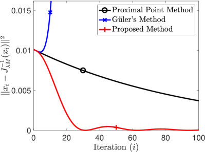
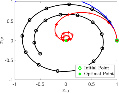
Figure 1: Solving a worst-case monotone inclusion problem of the proximal point method with $\bm{M}$ (40) with $N=100$; (left) the fixed-point residual vs. iteration, (right) the trajectory of the iterates $\bm{x}_{i}=[x_{i,1},\;x_{i,2}]^{\top}$ (markers are displayed every $5$th iterations).

We further investigate the behavior of the proposed method for a convex-concave saddle-point problem

$$\min_{\bm{u}\in\mathcal{H}_{1}}\max_{\bm{v}\in\mathcal{H}_{2}}\; \phi(\bm{u},\bm{v}),$$ (41)

where $\mathcal{H}_{1}$ and $\mathcal{H}_{2}$ denote real Hilbert spaces equipped with inner product $\mathop{\langle\cdot,\,\cdot\rangle}\nolimits$, and $\phi(\cdot,\bm{v})\in\mathcal{F}(\mathcal{H}_{1})$, $-\phi(\bm{u},\cdot)\in\mathcal{F}(\mathcal{H}_{2})$, which we further study in sections 5 and 6.1. The saddle subdifferential of $\phi$,

$$\left[\begin{array}[]{c}\partial_{\bm{u}}\phi(\bm{u},\bm{v})\\ \partial_{\bm{v}}(-\phi(\bm{u},\bm{v}))\end{array}\right],$$ (44)

is monotone rockafellar:70:moa . The proposed accelerated method applied to (44) with $\bm{x}_{i}:=(\bm{u}_{i},\bm{v}_{i})$ and $\bm{x}_{*}:=(\bm{u}_{*},\bm{v}_{*})$ (see Section 6.1 for details) satisfies

$$\phi(\bm{u}_{i},\bm{v}_{*})-\phi(\bm{u}_{*},\bm{v}_{i})\leq\frac{||\bm{u}_{0}-\bm{u}_{*}||^{2}+||\bm{v}_{0}-\bm{v}_{*}||^{2}}{4\lambda i}$$ (45)

for any $i\geq 1$. This is numerically conjectured by the PEP analysis in (19) with the objective function $\frac{1}{R}||\bm{x}_{N}-\bm{y}_{N-1}||^{2}$ and the inequality $\mathop{\langle\bm{x}_{N}-\bm{x}_{*},\,\bm{q}_{N}\rangle}\nolimits\geq 0$ in (19) replaced by $\phi(\bm{u}_{N},\bm{v}_{*})-\phi(\bm{u}_{*},\bm{v}_{N})$ and $\mathop{\langle\bm{x}_{N}-\bm{x}_{*},\,\bm{q}_{N}\rangle}\nolimits\geq\phi(\bm{u}_{N},\bm{v}_{*})-\phi(\bm{u}_{*},\bm{v}_{N})$, respectively.

5 Restarting the accelerated proximal point method for strongly monotone operators

For strongly monotone operators, the proximal point method has a linear rate (9), whereas the proposed accelerated method is not guaranteed to have such a fast rate. Technically, one should be able to find an accelerated method for strong monotone operators via PEP, as we did for the monotone operators in the previous section. However, the resulting PEP problem, a reminiscent of (HD), is much more difficult to solve, and we leave it as future work. Instead, we consider a fixed restarting technique in (nemirovski:94:emi, , Section 11.4)(nesterov:13:gmf, , Section 5.1) that restarts an accelerated method with a sublinear rate every certain number of iterations to yield a fast linear rate, particularly for $\bm{M}\in\mathcal{M}_{\mu}(\mathcal{H})$ in this section.

Suppose one restarts the proposed method every $k$ (inner) iterations by initializing the $(j+1)$th outer iteration $\bm{x}_{j+1,0}=\bm{y}_{j+1,0}=\bm{y}_{j+1,-1}$ by $\bm{x}_{j,k}$, where $\bm{x}_{j,l}$ and $\bm{y}_{j,l}$ denote iterates at the $j$th outer iteration and $l$th inner iteration for $j=0,1,\ldots$ and $l=-1,0,1,\ldots,k$. Using the rate (32) (with $R=||\bm{x}_{j,0}-\bm{x}_{*}||$) and the strong monotonicity condition (2), we have

$$||\bm{x}_{j,k}-\bm{y}_{j,k-1}||^{2}\leq\frac{||\bm{x}_{j,0}-\bm{x}_{*}||^{2}}{k^{2}}\leq\frac{1}{\mu^{2}k^{2}}||\bm{M}\bm{x}_{j,0}||^{2}$$ (46)

for $j=0,1,\ldots$. Since $\frac{1}{\lambda}(\bm{x}_{j-1,k}-\bm{y}_{j-1,k-1})\in\bm{M}\bm{x}_{j,0}$, we have a linear rate

$$||\bm{x}_{j,k}-\bm{y}_{j,k-1}||^{2}\leq\frac{1}{\lambda^{2}\mu^{2}k^{2}}||\bm{x}_{j-1,k}-\bm{y}_{j-1,k-1}||^{2}.$$ (47)

For a given $N=jk$ total number of steps, minimizing the overall rate with respect to $k$ yields an optimal choice of the restarting interval given by $k_{\mathrm{opt}}{\,\approx\,}\frac{e}{\lambda\mu}$, where $e$ is Euler’s number. The corresponding linear rate is $O((e^{\lambda\mu/e})^{-2N})$.

We further investigate the behavior of the restarting technique for a saddle-point problem (41) with an assumption that $\phi$ is strongly-convex-strongly-concave, i.e., $\phi(\cdot,\bm{v})-\frac{\mu}{2}||\cdot||^{2}\in\mathcal{F}(\mathcal{H}_{1})$ and $-\phi(\bm{u},\cdot)-\frac{\mu}{2}||\cdot||^{2}\in\mathcal{F}(\mathcal{H}_{2})$. The associated saddle subdifferential (44) is $\mu$-strongly monotone. For such case, using the rate (45), and the inequalities $\phi(\bm{u}_{*},\bm{v}_{*})+\frac{\mu}{2}||\bm{u}-\bm{u}_{*}||^{2}\leq\phi(\bm{u},\bm{v}_{*})$ and $-\phi(\bm{u}_{*},\bm{v}_{*})+\frac{\mu}{2}||\bm{v}-\bm{v}_{*}||^{2}\leq-\phi(\bm{u}_{*},\bm{v})$, the proposed method with restarting every $k$ iterations satisfies

$$\phi(\bm{u}_{j,k},\bm{v}_{*})-\phi(\bm{u}_{*},\bm{v}_{j,k})\leq\frac{1}{2\lambda\mu k}(\phi(\bm{u}_{j,0},\bm{v}_{*})-\phi(\bm{u}_{*},\bm{v}_{j,0}))$$ (48)

for $j=0,1,\ldots$. The associated optimal restarting interval is $k_{\mathrm{opt}}^{\phi}{\,\approx\,}\frac{e}{2\lambda\mu}$, which is twice smaller than $k_{\mathrm{opt}}$. The corresponding linear rate is also $O((e^{\lambda\mu/e})^{-2N})$, whereas the proximal point method has the rate $O((1+\lambda\mu)^{-2N})$ in (9). For any given positive $\mu$, there is no positive $\lambda$ that satisfies both $k_{\mathrm{opt}}^{\phi}(\lambda,\mu)\geq 1$ and $e^{\lambda\mu/e}>1+\lambda\mu$. This contrasts with the fact that the worst-case rate of optimally restarting the proposed method is not slower than that of the proximal point method. This implies that the bounds (47) and (48) are not exact, and we leave finding their tight bounds as future work. The numerical experiment below (and those in Section 6) suggests that the restarting technique can perform better than the proximal point method.

We consider a toy problem that is a combination of the worst-case problems in $\mathcal{M}(\mathcal{H})$ and $\mathcal{M}_{\mu}(\mathcal{H})$ for the proximal point method:

$$\bm{M}\left[\begin{array}[]{c}u\\ v\end{array}\right]=\left(\frac{1}{\lambda\sqrt{N-1}}\left[\begin{array}[]{cc}0&\;1\\ -1&\;0\end{array}\right]+\left[\begin{array}[]{cc}\mu&\;0\\ 0&\;\mu\end{array}\right]\right)\left[\begin{array}[]{c}u\\ v\end{array}\right],$$ (57)

which is the saddle subdifferential operator of $\phi(u,v)=\frac{\mu}{2}u^{2}+\frac{1}{\lambda\sqrt{N-1}}uv-\frac{\mu}{2}v^{2}$. We choose $N=100$, $\lambda=1$ and $\mu=0.02$. The optimal restarting intervals are $k_{\mathrm{opt}}\approx 136$ and $k_{\mathrm{opt}}^{\phi}\approx 68$, and we run $200$ iterations in the experiment, where restarting intervals $17$, $34$, $68$, and $136$ are considered. Figure 2 compares the proximal point method, its accelerated variants, and the proposed accelerated method with restarting, with an initial point $\bm{x}_{0}=[1\;0]^{\top}$ and the optimal point $\bm{x}_{*}=\bm{0}$. Figure 2 presents that the proximal point method has a linear rate that is faster than the proposed method (with a sublinear rate), while the restarting greatly accelerates the proposed method with a fast linear rate. Figure 2 also illustrates that the optimal restarting intervals $k_{\mathrm{opt}}$ and $k_{\mathrm{opt}}^{\phi}$ for strongly monotone operators and strongly-convex-strongly-concave functions, respectively, are not optimal for this specific case. Examples in the next section also present that the restarting can be useful even without strong monotonicity (but possibly with local strong monotonicity).

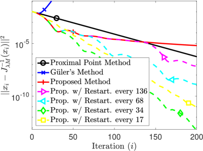
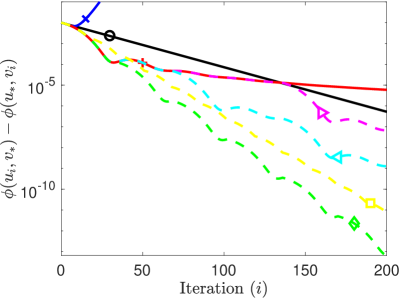
Figure 2: Solving a strongly monotone inclusion problem with $\bm{M}$ (57); (left) the fixed-point residual vs. iteration, (right) the function residual vs. iteration.

6 Applications of the accelerated proximal point method

As mentioned earlier, the proximal point method for maximally monotone operators include various well-known convex optimization methods. These include the augmented Lagrangian (i.e., the method of multipliers), the proximal method of multipliers, and ADMM. The augmented Lagrangian method is equivalent to the proximal point method directly solving the dual convex minimization problem rockafellar:76:ala , so Güler’s methods guler:92:npp already provide acceleration, whereas other instances of the proximal point method have no known accelerations yet. Thus, this section introduces accelerations to well-known instances of the proximal point method, which were not possible previously to the best of our knowledge (under this paper’s setting).

6.1 Accelerating the proximal point method for convex-concave saddle-point problem

This section considers a convex-concave saddle-point problem (41), where the associated saddle subdifferential operator (44) is monotone. rockafellar:76:moa applied the proximal point method on such operator to solve the convex-concave saddle-point problem, and this section further applies the proposed acceleration to such proximal point method as below.

Accelerated Proximal Point Method for Convex-Concave Saddle-Point Problem $\displaystyle\qquad\text{Input: }\phi(\cdot,\bm{v})\in\mathcal{F}(\mathcal{H}_{1}),\;-\phi(\bm{u},\cdot)\in\mathcal{F}(\mathcal{H}_{2}),\;\hat{\bm{u}}_{0}\in\mathcal{H}_{1},\;\hat{\bm{v}}_{0}\in\mathcal{H}_{2},$ $\displaystyle\qquad\qquad\quad\bm{x}_{0}=\bm{y}_{0}=\bm{y}_{-1}=(\hat{\bm{u}}_{0},\hat{\bm{v}}_{0}),\;\lambda\in\mathbbm{R}_{++}.$ $\displaystyle\qquad\text{For }i=0,1,\ldots$ $\displaystyle\qquad\qquad\bm{x}_{i+1}=(\bm{u}_{i+1},\bm{v}_{i+1})=\arg\min_{\bm{u}\in\mathcal{H}_{1}}\max_{\bm{v}\in\mathcal{H}_{2}}\left\{\phi(\bm{u},\bm{v})+\frac{1}{2\lambda}||\bm{u}-\hat{\bm{u}}_{i}||^{2}-\frac{1}{2\lambda}||\bm{v}-\hat{\bm{v}}_{i}||^{2}\right\},$ $\displaystyle\qquad\qquad\bm{y}_{i+1}=(\hat{\bm{u}}_{i+1},\hat{\bm{v}}_{i+1})=\bm{x}_{i+1}+\frac{i}{i+2}(\bm{x}_{i+1}-\bm{x}_{i})-\frac{i}{i+2}(\bm{x}_{i}-\bm{y}_{i-1}).$

One primary use of this accelerated method is the following convex-concave Lagrangian problem

$$\min_{\bm{u}\in\mathcal{H}_{1}}\max_{\bm{v}\in\mathcal{H}_{2}}\; \left\{L(\bm{u},\bm{v}):=f(\bm{u})+\mathop{\langle\bm{v},\,\bm{A}\bm{u}-\bm{b}\rangle}\nolimits\right\},$$ (58)

associated with the linearly constrained problem

$$\min_{\bm{u}\in\mathcal{H}_{1}}\; f(\bm{u})$$ (59)

subject to $$\bm{A}\bm{u}=\bm{b},$$

where $\bm{A}\in\mathcal{B}(\mathcal{H}_{1},\mathcal{H}_{2})$ and $\bm{b}\in\mathcal{H}_{2}$. The resulting method is called the proximal method of multipliers in rockafellar:76:ala , and applying the proposed acceleration to this method leads to below.

Accelerated Proximal Method of Multipliers $\displaystyle\qquad\text{Input: }\phi(\cdot,\bm{v})\in\mathcal{F}(\mathcal{H}_{1}),\;-\phi(\bm{u},\cdot)\in\mathcal{F}(\mathcal{H}_{2}),\;\hat{\bm{u}}_{0}\in\mathcal{H}_{1},\;\hat{\bm{v}}_{0}\in\mathcal{H}_{2},$ $\displaystyle\qquad\qquad\quad\bm{x}_{0}=\bm{y}_{0}=\bm{y}_{-1}=(\hat{\bm{u}}_{0},\hat{\bm{v}}_{0}),\;\lambda\in\mathbbm{R}_{++}.$ $\displaystyle\qquad\text{For }i=0,1,\ldots$ $\displaystyle\qquad\qquad\bm{u}_{i+1}=\arg\min_{\bm{u}\in\mathcal{H}_{1}}\left\{L(\bm{u},\hat{\bm{v}}_{i})+\frac{\lambda}{2}||\bm{A}\bm{u}-\bm{b}||^{2}+\frac{1}{2\lambda}||\bm{u}-\hat{\bm{u}}_{i}||^{2}\right\},$ $\displaystyle\qquad\qquad\bm{x}_{i+1}=(\bm{u}_{i+1},\hat{\bm{v}}_{i}+\lambda(\bm{A}\bm{u}_{i+1}-\bm{b})),$ $\displaystyle\qquad\qquad\bm{y}_{i+1}=(\hat{\bm{u}}_{i+1},\hat{\bm{v}}_{i+1})=\bm{x}_{i+1}+\frac{i}{i+2}(\bm{x}_{i+1}-\bm{x}_{i})-\frac{i}{i+2}(\bm{x}_{i}-\bm{y}_{i-1}).$

Note that this method without the acceleration and the term $\frac{1}{2\lambda}||\bm{u}-\bm{u}_{i}||^{2}$ reduces to the augmented Lagrangian method. This method has an advantage over the augmented Lagrangian method and its accelerated variants; the primal iterate $\bm{u}_{i+1}$ is uniquely defined with a better conditioning.

Example 1

We apply the accelerated proximal method of multipliers to a basis pursuit problem

$$\min_{\bm{u}\in\mathbbm{R}^{d_{1}}}\; ||\bm{u}||_{1}$$ (60)

subject to $$\bm{A}\bm{u}=\bm{b},$$

where $\bm{A}\in\mathbbm{R}^{d_{2}\times d_{1}}$ and $\bm{b}\in\mathbbm{R}^{d_{2}}$. In the experiment, we choose $d_{1}=100$, $d_{2}=20$, and randomly generated $\bm{A}$. A true sparse $\bm{u}_{\mathrm{true}}$ is randomly generated followed by a thresholding to sparsify nonzero elements, and $\bm{b}$ is then given by $\bm{A}\bm{u}_{\mathrm{true}}$. We run $100$ iterations of the proximal method of multipliers and its variants with $\lambda=0.01$ and initial $\bm{x}_{0}=\bm{0}$. Since the $\bm{u}_{i+1}$-update does not have a closed form, we used a sufficient number of iterations to solve the $\bm{u}_{i+1}$-update using the strongly convex version of FISTA beck:09:afi in (chambolle:16:ait, , Theorem 4.10).

Figure 3 compares the proximal method of multipliers and its accelerated variants. Similar to Fig. 1, Güler’s first accelerated version diverges, while the proposed method has accelerating behavior, compared to the non-accelerated version. The proposed method exhibits an oscillation in Fig. 3 (and a subtle oscillation in Fig. 1). This might be due to high momentum, owing from the acceleration, discussed in odonoghue:15:arf . So in Fig. 3 we heuristically restarted the method every $30$ iterations to avoid such oscillation and accelerate, as suggested in odonoghue:15:arf . Developing an approach to appropriately choosing a restarting interval or adaptively restarting the method as in odonoghue:15:arf for such problem are left as future work.

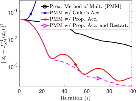
Figure 3: Solving a basis pursuit problem (60); the fixed-point residual vs. iteration.

6.2 Accelerating the primal-dual hybrid gradient method

This section considers a linearly coupled convex-concave saddle-point problem

$$\min_{\bm{u}\in\mathcal{H}_{1}}\max_{\bm{v}\in\mathcal{H}_{2}}\left\{\phi(\bm{u},\bm{v})\equiv f(\bm{u})+\mathop{\langle\bm{K}\bm{u},\,\bm{v}\rangle}\nolimits-g(\bm{v})\right\},$$ (61)

where $f\in\mathcal{F}(\mathcal{H}_{1})$, $g\in\mathcal{F}(\mathcal{H}_{2})$ and $\bm{K}\in\mathcal{B}(\mathcal{H}_{1},\mathcal{H}_{2})$. One widely known method for such problem is the primal-dual hybrid gradient (PDHG) method chambolle:11:afo ; esser:10:agf , which is a preconditioned proximal point method (with $\lambda=1$) for the saddle subdifferential operator of $\phi$ (44) chambolle:16:ote ; he:12:cao . The associated preconditioner is

$$\bm{P}=\left[\begin{array}[]{cc}\frac{1}{\tau}\bm{I}&\;-\bm{K}^{*}\\ -\bm{K}&\;\frac{1}{\sigma}\bm{I}\end{array}\right],$$ (64)

which is positive definite when $\tau\sigma||\bm{K}||^{2}<1$, where $||\bm{K}||=\sup_{||\bm{x}||\leq 1}||\bm{K}\bm{x}||$. As mentioned in remark 1, we can directly apply our results to the PDHG method as below.

Accelerated PDHG Method $\displaystyle\qquad\text{Input: }f\in\mathcal{F}(\mathcal{H}_{1}),\;g\in\mathcal{F}(\mathcal{H}_{2}),\;\bm{K}\in\mathcal{B}(\mathcal{H}_{1},\mathcal{H}_{2}),\;\hat{\bm{u}}_{0}\in\mathcal{H}_{1},\;\hat{\bm{v}}_{0}\in\mathcal{H}_{2},\;\tau\sigma||\bm{K}||^{2}<1,$ $\displaystyle\qquad\qquad\quad\bm{x}_{0}=\bm{y}_{0}=\bm{y}_{-1}=(\hat{\bm{u}}_{0},\hat{\bm{v}}_{0}).$ $\displaystyle\qquad\text{For }i=0,1,\ldots$ $\displaystyle\qquad\qquad\bm{u}_{i+1}=\mathop{\operator@font arg\,min}_{\bm{u}\in\mathcal{H}_{1}}\left\{f(\bm{u})+\mathop{\langle\bm{K}\bm{u},\,\hat{\bm{v}}_{i}\rangle}\nolimits+\frac{1}{2\tau}||\bm{u}-\hat{\bm{u}}_{i}||^{2}\right\}$ $\displaystyle\qquad\qquad\bm{v}_{i+1}=\mathop{\operator@font arg\,min}_{\bm{v}\in\mathcal{H}_{2}}\left\{g(\bm{v})-\mathop{\langle\bm{K}(2\bm{u}_{i+1}-\hat{\bm{u}}_{i}),\,\bm{v}\rangle}\nolimits+\frac{1}{2\sigma}||\bm{v}-\hat{\bm{v}}_{i}||^{2}\right\}$ $\displaystyle\qquad\qquad\bm{x}_{i+1}=(\bm{u}_{i+1},\bm{v}_{i+1})$ $\displaystyle\qquad\qquad\bm{y}_{i+1}=(\hat{\bm{u}}_{i+1},\hat{\bm{v}}_{i+1})=\bm{x}_{i+1}+\frac{i}{i+2}(\bm{x}_{i+1}-\bm{x}_{i})-\frac{i}{i+2}(\bm{x}_{i}-\bm{y}_{i-1})$

Corollary 1

Assume that $\mathop{\langle\bm{P}(\bm{x}_{0}-\bm{x}_{*}),\,\bm{x}_{0}-\bm{x}_{*}\rangle}\nolimits\leq R^{2}$ for some $\bm{x}_{*}\in X_{*}(\bm{M})$. The PDHG method satisfies

$$\mathop{\langle\bm{P}(\bm{x}_{i}-\bm{x}_{i-1}),\,\bm{x}_{i}-\bm{x}_{i-1}\rangle}\nolimits\leq\left(1-\frac{1}{i}\right)^{i-1}\frac{R^{2}}{i},$$

and the proposed accelerated PDHG method satisfies

$$\mathop{\langle\bm{P}(\bm{x}_{i}-\bm{y}_{i-1}),\,\bm{x}_{i}-\bm{y}_{i-1}\rangle}\nolimits\leq\frac{R^{2}}{i^{2}}.$$

Example 2

We apply the accelerated PDHG method to the bilinear game problem

$$\min_{\bm{u}\in\mathbbm{R}^{d_{1}}}\max_{\bm{v}\in\mathbbm{R}^{d_{2}}}\mathop{\langle\bm{a},\,\bm{u}\rangle}\nolimits+\mathop{\langle\bm{K}\bm{u},\,\bm{v}\rangle}\nolimits-\mathop{\langle\bm{b},\,\bm{v}\rangle}\nolimits,$$ (65)

where $\bm{K}\in\mathbbm{R}^{d_{2}\times d_{1}}$, $\bm{a}\in\mathbbm{R}^{d_{1}}$ and $\bm{b}\in\mathbbm{R}^{d_{2}}$. The main part of the corresponding method is as below:

$$\bm{u}_{i+1} =\hat{\bm{u}}_{i}-\tau(\bm{K}^{*}\hat{\bm{v}}_{i}+\bm{a})$$ (66)

$$\bm{v}_{i+1} =\hat{\bm{v}}_{i}+\sigma(\bm{K}(2\bm{u}_{i+1}-\hat{\bm{u}}_{i})-\bm{b}).$$

In the experiment, we choose $d_{1}=1000$, $d_{2}=500$, and a matrix $\bm{K}$ and vectors $\bm{a},\bm{b}$ are randomly generated. We run $100$ iterations of the PDHG method and its variants with initial $\hat{\bm{u}}_{0}=[10\;\cdots\;10]^{\top}$, $\hat{\bm{v}}_{0}=[10\;\cdots\;10]^{\top}$ and $\tau=\sigma=\frac{0.99}{||\bm{K}||}$. Figure 4 plots the preconditioned fixed-point residual, where Güler’s first accelerated method diverges. The PDHG method and its proposed accelerated variant are comparable in this experiment, and heuristically restarting the accelerated method every $10$ iterations yields a big acceleration. While chambolle:11:afo found restarting (reinitializing) a relaxed PDHG method not useful, our experiment suggests that restarting can be effective in some practical cases.

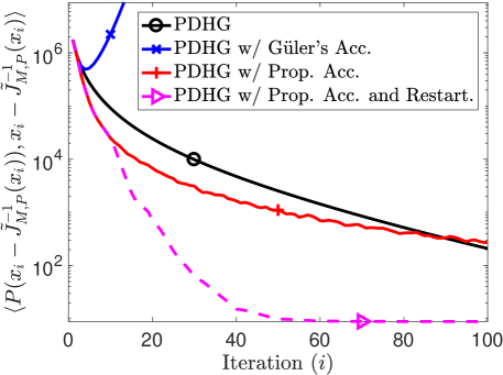
Figure 4: Solving a bilinear game problem (65) by a preconditioned proximal point method; the preconditioned fixed-point residual vs. iteration. $\tilde{\bm{J}}_{\bm{M},\bm{P}}:=(\bm{P}+\bm{M})^{-1}\bm{P}$ denotes the preconditioned resolvent operator.

6.3 Accelerating the Douglas-Rachford splitting method

This section considers a monotone inclusion problem in a form

$$\operatorname{Find}\;\;\bm{x}\in\mathcal{H}\quad\text{subject to}\quad\bm{0}\in(\bm{M}_{1}+\bm{M}_{2})\bm{x}$$ (67)

for $\bm{M}_{1},\bm{M}_{2}\in\mathcal{M}(\mathcal{H})$, where $\bm{J}_{\rho\bm{M}_{1}}$ and $\bm{J}_{\rho\bm{M}_{2}}$ are more efficient than $\bm{J}_{\rho(\bm{M}_{1}+\bm{M}_{2})}$ for a positive real number $\rho$. For such problem, the Douglas-Rachford splitting method douglas:56:otn ; lions:79:saf that iteratively applies the operator

$$\bm{G}_{\rho,\bm{M}_{1},\bm{M}_{2}}:=\bm{J}_{\rho\bm{M}_{1}}\circ(2\bm{J}_{\rho\bm{M}_{2}}-\bm{I})+(\bm{I}-\bm{J}_{\rho\bm{M}_{2}})$$ (68)

has been found to be effective in many applications including ADMM, which we discuss in the next section.

In (eckstein:92:otd, , Theorem 4), the Douglas-Rachford operator (68) was found to be a resolvent $\bm{J}_{\bm{M}_{\rho,\bm{M}_{1},\bm{M}_{2}}}$ of a maximally monotone operator

$$\bm{M}_{\rho,\bm{M}_{1},\bm{M}_{2}}:=\bm{G}_{\rho,\bm{M}_{1},\bm{M}_{2}}^{-1}-\bm{I}.$$ (69)

In other words, the Douglas-Rachford splitting method is an instance of the proximal point method (with $\lambda=1$) as

$$\bm{\nu}_{i+1}=\bm{J}_{\bm{M}_{\rho,\bm{M}_{1},\bm{M}_{2}}}(\bm{\nu}_{i})=\bm{G}_{\rho,\bm{M}_{1},\bm{M}_{2}}(\bm{\nu}_{i})$$ (70)

for $i=0,1,\ldots$. Therefore, we can apply the proposed acceleration to the Douglas-Rachford splitting method as below.

Accelerated Douglas-Rachford Splitting Method $\displaystyle\qquad\text{Input: }\bm{M}_{1},\bm{M}_{2}\in\mathcal{M}(\mathcal{H}),\;\bm{\nu}_{0}=\bm{\eta}_{0}=\bm{\eta}_{-1}\in\mathcal{H},\;\rho\in\mathbbm{R}_{++}.$ $\displaystyle\qquad\text{For }i=0,1,\ldots$ $\displaystyle\qquad\qquad\bm{\nu}_{i+1}=\bm{G}_{\rho,\bm{M}_{1},\bm{M}_{2}}(\bm{\eta}_{i})$ $\displaystyle\qquad\qquad\bm{\eta}_{i+1}=\bm{\nu}_{i+1}+\frac{i}{i+2}(\bm{\nu}_{i+1}-\bm{\nu}_{i})-\frac{i}{i+2}(\bm{\nu}_{i}-\bm{\eta}_{i-1})$

Using (8) and (32), we have the following worst-case rates for the Douglas-Rachford splitting method and its accelerated variant. Finding exact bounds for the Douglas-Rachford splitting method and its variant is left as future work; ryu:20:osp used PEP to analyze the exact worst-case rate of Douglas-Rachford splitting method under some additional conditions.

Corollary 2

Assume that $||\bm{\nu}_{0}-\bm{\nu}_{*}||\leq R$ for some $\bm{\nu}_{*}\in X_{*}(\bm{M}_{\rho,\bm{M}_{1},\bm{M}_{2}})$. The Douglas-Rachford splitting method satisfies

$$||\bm{\nu}_{i}-\bm{\eta}_{i-1}||^{2}\leq\left(1-\frac{1}{i}\right)^{i-1}\frac{R^{2}}{i},$$ (71)

and the proposed accelerated Douglas-Rachford splitting method satisfies

$$||\bm{\nu}_{i}-\bm{\eta}_{i-1}||^{2}\leq\frac{R^{2}}{i^{2}}.$$ (72)

eckstein:88:tlm ; eckstein:92:otd illustrated that ADMM is equivalent to the Douglas-Rachford splitting method on the dual problem, so we naturally develop an accelerated ADMM in the next section and provide numerical experiment of the accelerated ADMM and thus the accelerated Douglas-Rachford splitting method.

6.4 Accelerating the alternating direction method of multipliers (ADMM)

Let $\mathcal{H}_{1},\mathcal{H}_{2},\mathcal{G}$ be real Hilbert spaces equipped with inner product $\mathop{\langle\cdot,\,\cdot\rangle}\nolimits$. This section considers a linearly constrained convex problem

$$\min_{\bm{x}\in\mathcal{H}_{1},\bm{z}\in\mathcal{H}_{2}}\; f(\bm{x})+g(\bm{z})$$ (73)

subject to $$\bm{A}\bm{x}+\bm{B}\bm{z}=\bm{c},$$

where $f\in\mathcal{F}(\mathcal{H}_{1})$, $g\in\mathcal{F}(\mathcal{H}_{2})$, $\bm{A}\in\mathcal{B}(\mathcal{H}_{1},\mathcal{G})$, $\bm{B}\in\mathcal{B}(\mathcal{H}_{2},\mathcal{G})$ and $\bm{c}\in\mathcal{G}$. Its dual problem is

$$\max_{\bm{\nu}\in\mathcal{G}}\; \left\{-f^{*}(-\bm{A}^{*}\bm{\nu})-g^{*}(-\bm{B}^{*}\bm{\nu})+\mathop{\langle\bm{c},\,\bm{\nu}\rangle}\nolimits\right\},$$ (74)

where $f^{*}(\bm{y}):=\sup_{\bm{x}\in\mathcal{H}_{1}}\{\mathop{\langle\bm{y},\,\bm{x}\rangle}\nolimits-f(\bm{x})\}$ and $g^{*}(\bm{y}):=\sup_{\bm{z}\in\mathcal{H}_{2}}\{\mathop{\langle\bm{y},\,\bm{z}\rangle}\nolimits-g(\bm{z})\}$ are the conjugate functions of $f$ and $g$, respectively. The dual problem (74) is equivalent to the following monotone inclusion problem

$$\operatorname{Find}\;\;\bm{\nu}\in\mathcal{G}\quad\text{subject to}\quad\bm{0}\in-\bm{A}\partial f^{*}(-\bm{A}^{*}\bm{\nu})-\bm{B}\partial g^{*}(-\bm{B}^{*}\bm{\nu})-\bm{c}.$$ (75)

We next use the connection between ADMM for solving (73) and the Douglas-Rachford splitting method for solving (75) in (davis:16:cra, , Proposition 9)ryu:16:apo to develop an accelerated ADMM, using the accelerated Douglas-Rachford splitting method in the previous section.

Denoting

$$\bm{M}_{1} :=-\bm{A}\partial f^{*}(-\bm{A}^{*}\cdot)-\bm{c}\quad\text{and}\quad\bm{M}_{2}:=-\bm{B}\partial g^{*}(-\bm{B}^{*}\cdot)$$ (76)

converts the problem (75) into a form of the monotone inclusion problem (67). Then we use the following equivalent form of the accelerated Douglas-Rachford splitting method to solve (67) with (76):

$$\bm{\zeta}_{i+1} =\bm{J}_{\rho\bm{M}_{2}}(\bm{\eta}_{i})$$ (77)

$$\bm{\xi}_{i+1} =\bm{J}_{\rho\bm{M}_{1}}(2\bm{\zeta}_{i+1}-\bm{\eta}_{i})$$

$$\bm{\nu}_{i+1} =\bm{\eta}_{i}+(\bm{\xi}_{i+1}-\bm{\zeta}_{i})$$

$$\bm{\eta}_{i+1} =\bm{\nu}_{i+1}+\frac{i}{i+2}(\bm{\nu}_{i+1}-\bm{\nu}_{i})-\frac{i}{i+2}(\bm{\nu}_{i}-\bm{\eta}_{i-1})$$

for $i=0,1,\ldots$. Replacing the resolvent operators of $\bm{M}_{1}$ and $\bm{M}_{2}$ in (76) by minimization steps yields

$$\bm{z}_{i+1} =\mathop{\operator@font arg\,min}_{\bm{z}\in\mathcal{H}_{2}}\left\{g(\bm{z})+\mathop{\langle\bm{\eta}_{i},\,\bm{B}\bm{z}\rangle}\nolimits+\frac{\rho}{2}||\bm{B}\bm{z}||^{2}\right\}$$ (78)

$$\bm{\zeta}_{i+1} =\bm{\eta}_{i}+\rho\bm{B}\bm{z}_{i+1}$$

$$\tilde{\bm{x}}_{i+1} =\mathop{\operator@font arg\,min}_{\bm{x}\in\mathcal{H}_{1}}\left\{f(\bm{x})+\mathop{\langle\bm{\eta}_{i}+2\rho\bm{B}\bm{z}_{i+1},\,\bm{A}\bm{x}-\bm{c}\rangle}\nolimits+\frac{\rho}{2}||\bm{A}\bm{x}-\bm{c}||^{2}\right\}$$

$$\bm{\xi}_{i+1} =\bm{\eta}_{i}+\rho(\bm{A}\tilde{\bm{x}}_{i+1}-\bm{c})+2\rho\bm{B}\bm{z}_{i+1}$$

$$\bm{\nu}_{i+1} =\bm{\eta}_{i}+\rho(\bm{A}\tilde{\bm{x}}_{i+1}+\bm{B}\bm{z}_{i+1}-\bm{c})$$

$$\bm{\eta}_{i+1} =\bm{\nu}_{i+1}+\frac{i}{i+2}(\bm{\nu}_{i+1}-\bm{\nu}_{i})-\frac{i}{i+2}(\bm{\nu}_{i}-\bm{\eta}_{i-1}).$$

By discarding $\bm{\zeta}_{i}$ and $\bm{\xi}_{i}$, and defining

$$\hat{\bm{\nu}}_{i}:=\bm{\nu}_{i}-\rho(\bm{A}\tilde{\bm{x}}_{i}-\bm{c})\quad\text{and}\quad\hat{\bm{\eta}}_{i}:=\bm{\eta}_{i}-\rho(\bm{A}\tilde{\bm{x}}_{i}-\bm{c}),$$ (79)

for $i=0,1,\ldots$, we have

$$\bm{z}_{i+1} =\mathop{\operator@font arg\,min}_{\bm{z}\in\mathcal{H}_{2}}\left\{g(\bm{z})+\mathop{\langle\hat{\bm{\eta}}_{i}+\rho(\bm{A}\tilde{\bm{x}}_{i}-\bm{c}),\,\bm{B}\bm{z}\rangle}\nolimits+\frac{\rho}{2}||\bm{B}\bm{z}||^{2}\right\}$$ (80)

$$=\mathop{\operator@font arg\,min}_{\bm{z}\in\mathcal{H}_{2}}\left\{g(\bm{z})+\mathop{\langle\hat{\bm{\eta}}_{i},\,\bm{A}\tilde{\bm{x}}_{i}+\bm{B}\bm{z}-\bm{c}\rangle}\nolimits+\frac{\rho}{2}||\bm{A}\tilde{\bm{x}}_{i}+\bm{B}\bm{z}-\bm{c}||^{2}\right\}$$

$$\tilde{\bm{x}}_{i+1} =\mathop{\operator@font arg\,min}_{\bm{x}\in\mathcal{H}_{1}}\left\{f(\bm{x})+\mathop{\langle\hat{\bm{\nu}}_{i+1}+\rho\bm{B}\bm{z}_{i+1},\,\bm{A}\bm{x}-\bm{c}\rangle}\nolimits+\frac{\rho}{2}||\bm{A}\bm{x}-\bm{c}||^{2}\right\}$$

$$=\mathop{\operator@font arg\,min}_{\bm{x}\in\mathcal{H}_{1}}\left\{f(\bm{x})+\mathop{\langle\hat{\bm{\nu}}_{i+1},\,\bm{A}\bm{x}+\bm{B}\bm{z}_{i+1}-\bm{c}\rangle}\nolimits+\frac{\rho}{2}||\bm{A}\bm{x}+\bm{B}\bm{z}_{i+1}-\bm{c}||^{2}\right\}$$

$$\hat{\bm{\nu}}_{i+1} =\hat{\bm{\eta}}_{i}+\rho(\bm{A}\tilde{\bm{x}}_{i}+\bm{B}\bm{z}_{i+1}-\bm{c})$$

$$\hat{\bm{\eta}}_{i+1} =\hat{\bm{\nu}}_{i+1}+\frac{i}{i+2}(\hat{\bm{\nu}}_{i+1}-\hat{\bm{\nu}}_{i}+\rho\bm{A}(\tilde{\bm{x}}_{i+1}-\tilde{\bm{x}}_{i}))-\frac{i}{i+2}(\hat{\bm{\nu}}_{i}-\hat{\bm{\eta}}_{i-1}+\rho\bm{A}(\tilde{\bm{x}}_{i}-\tilde{\bm{x}}_{i-1})).$$

Then, replacing $\tilde{\bm{x}}_{i}$ by $\bm{x}_{i+1}$ and reordering steps appropriately yield the following accelerated version of ADMM, which reduces to the standard ADMM when we let $\hat{\bm{\eta}}_{i}=\hat{\bm{\nu}}_{i}$ for $i=0,1,\ldots$.

Accelerated Alternating Direction Method of Multipliers $\displaystyle\qquad\text{Input: }f\in\mathcal{F}(\mathcal{H}_{1}),\;g\in\mathcal{F}(\mathcal{H}_{2}),\;\bm{A}\in\mathcal{B}(\mathcal{H}_{1},\mathcal{G}),\;\bm{B}\in\mathcal{B}(\mathcal{H}_{2},\mathcal{G}),\;\bm{x}_{0}\in\mathcal{H}_{1},\;\bm{z}_{0}\in\mathcal{H}_{2},\;\hat{\bm{\nu}}_{0}\in\mathcal{G},\;\rho\in\mathbbm{R}_{++}.$ $\displaystyle\qquad\text{For }i=0,1,\ldots$ $\displaystyle\qquad\qquad\bm{x}_{i+1}=\mathop{\operator@font arg\,min}_{\bm{x}\in\mathcal{H}_{1}}\left\{f(\bm{x})+\mathop{\langle\hat{\bm{\nu}}_{i},\,\bm{A}\bm{x}+\bm{B}\bm{z}_{i}-\bm{c}\rangle}\nolimits+\frac{\rho}{2}||\bm{A}\bm{x}+\bm{B}\bm{z}_{i}-\bm{c}||^{2}\right\}$ $\displaystyle\qquad\qquad\hat{\bm{\eta}}_{i}=\begin{cases}\hat{\bm{\nu}}_{i}&i=0,1,\\ \hat{\bm{\nu}}_{i}+\frac{i-1}{i+1}(\hat{\bm{\nu}}_{i}-\hat{\bm{\nu}}_{i-1}+\rho\bm{A}(\bm{x}_{i+1}-\bm{x}_{i}))-\frac{i-1}{i+1}(\hat{\bm{\nu}}_{i-1}-\hat{\bm{\eta}}_{i-2}+\rho\bm{A}(\bm{x}_{i}-\bm{x}_{i-1})),&i=2,3,\ldots\end{cases}$ $\displaystyle\qquad\qquad\bm{z}_{i+1}=\mathop{\operator@font arg\,min}_{\bm{z}\in\mathcal{H}_{2}}\left\{g(\bm{z})+\mathop{\langle\hat{\bm{\eta}}_{i},\,\bm{A}\bm{x}_{i+1}+\bm{B}\bm{z}-\bm{c}\rangle}\nolimits+\frac{\rho}{2}||\bm{A}\bm{x}_{i+1}+\bm{B}\bm{z}-\bm{c}||^{2}\right\}$ $\displaystyle\qquad\qquad\hat{\bm{\nu}}_{i+1}=\hat{\bm{\eta}}_{i}+\rho(\bm{A}\bm{x}_{i+1}+\bm{B}\bm{z}_{i+1}-\bm{c})$

Since

$$\bm{\nu}_{i}-\bm{\eta}_{i-1}=\hat{\bm{\nu}}_{i}-\hat{\bm{\eta}}_{i-1}-\rho(\bm{A}\bm{x}_{i+1}-\bm{A}\bm{x}_{i})=\rho(\bm{A}\bm{x}_{i+1}+\bm{B}\bm{z}_{i}-\bm{c}),$$ (81)

we have the following worst-case rates with respect to the infeasibility for ADMM and its accelerated version, using (8) and (32).

Corollary 3

Assume that $||\hat{\bm{\nu}}_{0}+\rho\bm{A}(\bm{x}_{0}-\bm{c})-\bm{\nu}_{*}||\leq R$ for some $\bm{\nu}_{*}\in X_{*}(\bm{M}_{\rho,-\bm{A}\partial f^{*}(-\bm{A}^{*}\cdot)-\bm{c},-\bm{B}\partial g^{*}(-\bm{B}^{*}\cdot)})$. Alternating direction method of multipliers satisfies

$$||\bm{A}\bm{x}_{i+1}+\bm{B}\bm{z}_{i}-\bm{c}||^{2}\leq\left(1-\frac{1}{i}\right)^{i-1}\frac{R^{2}}{\rho^{2}i},$$ (82)

and the proposed accelerated alternating direction method of multipliers satisfies

$$||\bm{A}\bm{x}_{i+1}+\bm{B}\bm{z}_{i}-\bm{c}||^{2}\leq\frac{R^{2}}{\rho^{2}i^{2}}.$$ (83)

The bound (82) is $e$-times asymptotically smaller than the known rate for ADMM in (davis:16:cra, , Theorem 15), which originated from the bound (7). Finding exact bounds for the ADMM and its proposed variant is yet left as future work.

Remark 2

Many existing rates for the (preconditioned) ADMM consider the ergodic sequences $\{\bar{\bm{x}}_{i}\}$ and $\{\bar{\bm{z}}_{i}\}$, where $\bar{\bm{x}}_{i}:=\frac{1}{i}\sum_{l=1}^{i}\bm{x}_{l}$ and $\bar{\bm{z}}_{i}:=\frac{1}{i}\sum_{l=1}^{i}\bm{z}_{l}$ (see e.g., chambolle:11:afo ; chambolle:16:ote ; davis:16:cra ; davis:17:fcr ). In particular, in (davis:16:cra, , Theorem 15), ADMM is found to satisfy

$$||\bm{A}\bar{\bm{x}}_{i+1}+\bm{B}\bar{\bm{z}}_{i}-\bm{c}||^{2}\leq\frac{16R^{2}}{\rho^{2}i^{2}},$$ (84)

which is faster than the rate of the nonergodic sequence $\{\bm{x}_{i},\bm{z}_{i}\}$ of ADMM in (82) and is comparable to the rate of the proposed accelerated ADMM in (83). One should note that the feasibility convergence of the ergodic sequence, as in (84), does not necessarily imply the convergence of the fixed-point residual of the ergodic sequence, unlike (82) and (83) for the nonergodic sequence. In addition, some numerical experiments in chambolle:16:ote illustrate that the performance of the nonergodic sequence can be faster than that of the ergodic sequence. We leave further understanding the rates of the ergodic and nonergodic sequences of (preconditioned) ADMM and their relationship as future work.

Remark 3

chambolle:11:afo ; chambolle:16:ote ; goldstein:14:fad proposed accelerated variants of (preconditioned) ADMM under some additional conditions, while the proposed method does not require such conditions.

Example 3

We apply the accelerated ADMM to the problem

$$\min_{\bm{x}\in\mathbbm{R}^{d_{1}},\bm{z}\in\mathbbm{R}^{d_{2}}}\; \frac{1}{2}||\bm{H}\bm{x}-\bm{b}||^{2}+\gamma||\bm{z}||_{1}$$ (85)

subject to $$\bm{D}\bm{x}-\bm{z}=\bm{0},$$

with a positive real number $\gamma$, associated with the total-variation-regularized least-squares problem

$$\min_{\bm{x}\in\mathbbm{R}^{d_{1}}}\; \frac{1}{2}||\bm{H}\bm{x}-\bm{b}||^{2}+\gamma||\bm{D}\bm{x}||_{1},$$ (86)

where $\bm{H}\in\mathbbm{R}^{p\times d_{1}}$, $\bm{b}\in\mathbbm{R}^{p}$, and a matrix $\bm{D}\in\mathbbm{R}^{d_{2}\times d_{1}}$ is given as

$$\bm{D}=\left[\begin{array}[]{cccccc}1&-1&0&0&\cdots&0\\ 0&1&-1&0&\cdots&0\\ \vdots&\ddots&\ddots&\ddots&\ddots&\vdots\\ \vdots&\ddots&0&1&-1&0\\ 0&\cdots&\cdots&0&1&-1\end{array}\right].$$ (92)

By letting $f(\bm{x})=\frac{1}{2}||\bm{H}\bm{x}-\bm{b}||^{2}$, $g(\bm{z})=\gamma||\bm{z}||_{1}$, $\bm{A}=\bm{D}$, $\bm{B}=-\bm{I}$ and $\bm{c}=\bm{0}$, we have the following accelerated ADMM method:

$$\bm{x}_{i+1} =\mathop{\operator@font arg\,min}_{\bm{x}\in\mathbbm{R}^{d_{1}}}\left\{\frac{1}{2}||\bm{H}\bm{x}-\bm{b}||^{2}+\mathop{\langle\hat{\bm{\nu}}_{i},\,\bm{D}\bm{x}-\bm{z}_{i}\rangle}\nolimits+\frac{\rho}{2}||\bm{D}\bm{x}-\bm{z}_{i}||^{2}\right\}$$ (93)

$$=(\bm{H}^{\top}\bm{H}+\rho\bm{D}^{\top}\bm{D})^{-1}(\bm{D}^{\top}(\rho\bm{z}_{i}-\hat{\bm{\nu}}_{i})+\bm{H}^{\top}\bm{b})$$

$$\hat{\bm{\eta}}_{i} =\begin{cases}\hat{\bm{\nu}}_{i},&i=0,1,\\ \hat{\bm{\nu}}_{i}+\frac{i-1}{i+1}(\hat{\bm{\nu}}_{i}-\hat{\bm{\nu}}_{i-1}+\rho\bm{D}(\bm{x}_{i+1}-\bm{x}_{i}))-\frac{i-1}{i+1}(\hat{\bm{\nu}}_{i-1}-\hat{\bm{\eta}}_{i-2}+\rho\bm{D}(\bm{x}_{i}-\bm{x}_{i-1})),&i=2,3,\ldots\end{cases}$$

$$\bm{z}_{i+1} =\mathop{\operator@font arg\,min}_{\bm{z}\in\mathbbm{R}^{d_{2}}}\left\{\gamma||\bm{z}||_{1}+\mathop{\langle\hat{\bm{\eta}}_{i},\,\bm{D}\bm{x}_{i+1}-\bm{z}\rangle}\nolimits+\frac{\rho}{2}||\bm{D}\bm{x}_{i+1}-\bm{z}||^{2}\right\}=\operatorname{S}_{\frac{\gamma}{\rho}}\left(\bm{D}\bm{x}_{i+1}+\frac{1}{\rho}\hat{\bm{\eta}}_{i}\right)$$

$$\hat{\bm{\nu}}_{i+1} =\hat{\bm{\eta}}_{i}+\rho(\bm{D}\bm{x}_{i+1}-\bm{z}_{i+1}),$$

where the soft-thresholding operator is defined as $\operatorname{S}_{\tau}(\bm{z}):=\max\{|\bm{z}|-\tau,\bm{0}\}\odot\operatorname{sign}(\bm{z})$ with the element-wise absolute value, maximum and multiplication operators, $|\cdot|$, $\max\{\cdot,\cdot\}$ and $\odot$, respectively.

In the experiment, we choose $d_{1}=100$, $d_{2}=99$, $p=5$, and a true vector $\bm{x}_{\mathrm{true}}$ is constructed such that a vector $\bm{D}\bm{x}_{\mathrm{true}}$ has few nonzero elements. A matrix $\bm{H}$ is randomly generated and a noisy vector $\bm{b}$ is generated by adding randomly generated (noise) vector to $\bm{H}\bm{x}_{\mathrm{true}}$. We choose the parameters $\gamma=3$ and $\rho=0.05$ in the experiment.

Figure 5 illustrates the fixed-point residual of ADMM and its accelerated variants. Interestingly, ADMM has a rate comparable to the $O(1/i^{2})$ rate of the proposed method. This does not contradict with the theory, and we leave further investigating the worst-case rate of ADMM under the Lipschitz continuity condition of $\nabla f$; similar analysis but under different conditions can be found in davis:16:cra ; davis:17:fcr . Noticing the oscillating behavior of the proposed ADMM in Fig. 5, we heuristically restarted the proposed method every $20$ iterations, yielding a linear rate, without a strong monotonicity condition. Restarting has been previously found useful for a different accelerated ADMM in goldstein:14:fad .

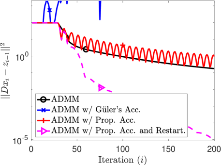
Figure 5: Solving a total-variation-regularized least-squares problem (86); the fixed-point residual vs. iteration

7 Accelerated forward method for cocoercive operators

This section applies the proposed acceleration to a forward method, such as a gradient method, for cocoercive operators. A single-valued operator $\bm{M}\;:\;\mathcal{H}\to\mathcal{H}$ is $\beta$-cocoercive for $\beta\in\mathbbm{R}_{++}$ if

$$\mathop{\langle\bm{x}-\bm{y},\,\bm{M}\bm{x}-\bm{M}\bm{y}\rangle}\nolimits\geq\beta||\bm{M}\bm{x}-\bm{M}\bm{y}||^{2}\text{ for all }\bm{x},\bm{y}\in\mathcal{H}.$$ (94)

Let $\mathcal{C}_{\beta}(\mathcal{H})$ be the class of $\beta$-cocoercive operators on $\mathcal{H}$. For the $\beta$-cocoercive operator, the following forward method (that iteratively applies the forward operator $\bm{I}-\beta\bm{M}$) is guaranteed to converge weakly to a solution (bauschke:11:caa, , Theorem 26.14).

Forward Method $\displaystyle\qquad\text{Input: }\bm{M}\in\mathcal{C}_{\beta}(\mathcal{H}),\;\bm{y}_{0}\in\mathcal{H}.$ $\displaystyle\qquad\text{For }i=0,1,\ldots$ $\displaystyle\qquad\qquad\bm{y}_{i+1}=(\bm{I}-\beta\bm{M})\bm{y}_{i}.$

An operator $\bm{T}\;:\;\mathcal{H}\to\mathcal{H}$ is $\lambda$-cocoercive if and only if it is the Yosida approximation of index $\lambda$ (bauschke:11:caa, , Proposition 23.21):

$$\bm{M}_{\lambda}:=\frac{1}{\lambda}(\bm{I}-\bm{J}_{\lambda\bm{M}})$$ (95)

of a maximally monotone operator $\bm{M}\;:\;\mathcal{H}\to 2^{\mathcal{H}}$. We thus have the following equivalence between the resolvent (backward) operator of a maximally monotone operator $\bm{M}$ and a forward operator of the corresponding cocoercive operator $\bm{M}_{\lambda}$:

$$\bm{J}_{\lambda\bm{M}}=(\bm{I}+\lambda\bm{M})^{-1}=\bm{I}-\lambda\bm{M}_{\lambda}.$$ (96)

Therefore, the results on the proximal point method and its accelerated variant for monotone operators directly apply to the forward method and its accelerated variant for cocoercive operators.

8 Conclusion

This paper developed an accelerated proximal point method for maximally monotone operators, with respect to the fixed-point residual, using the computer-assisted performance estimation problem approach. Restarting technique was further employed under the strong monotonicity condition. The proposed acceleration was applied to various instances of the proximal point method such as the proximal method of multipliers, the primal-dual hybrid gradient method, the Douglas-Rachford splitting method, and the alternating direction method of multipliers, yielding accelerations both theoretically and practically. The acceleration was also applied to a forward method for cocoercive operators.

We leave developing accelerations for more general or more specific classes of problems or methods as future work, possibly via the performance estimation problem approach; a comprehensive understanding of accelerations for the alternating direction method of multipliers with respect to various performance measures under various conditions are yet remain open.

- (1) Alvarez, F., Attouch, H.: An inertial proximal method for maximal monotone operators via discretization of a nonlinear oscillator with damping. Set-Valued Analysis 9(1–2), 3–11 (2001). DOI 10.1023/A:1011253113155
- (2) Attouch, H., Cabot, A.: Convergence of a relaxed inertial forward-backward algorithm for structured monotone inclusions. Appl. Math. Optim. 80(3), 547–598 (2019). DOI 10.1007/s00245-019-09584-z
- (3) Attouch, H., Cabot, A.: Convergence of a relaxed inertial proximal algorithm for maximally monotone operators. Mathematical Programming 184(1–2), 243–287 (2020). DOI 10.1007/s10107-019-01412-0
- (4) Attouch, H., Chbani, Z., Fadili, J., Riahi, H.: First-order optimization algorithms via inertial systems with Hessian driven damping. Mathematical Programming (2020). DOI 10.1007/s10107-020-01591-1
- (5) Attouch, H., Chbani, Z., Riahi, H.: Fast proximal methods via time scaling of damped inertial dynamics. SIAM J. Optim. 29(3), 2227–2256 (2019). DOI 10.1137/18M1230207
- (6) Attouch, H., Peypouquet, J.: Convergence of inertial dynamics and proximal algorithms governed by maximally monotone operators. Mathematical Programming 174(1–2), 391–432 (2019). DOI 10.1007/s10107-018-1252-x
- (7) Bauschke, H.H., Combettes, P.L.: Convex analysis and monotone operator theory in Hilbert spaces. Springer (2011). DOI 10.1007/978-1-4419-9467-7
- (8) Beck, A., Teboulle, M.: A fast iterative shrinkage-thresholding algorithm for linear inverse problems. SIAM J. Imaging Sci. 2(1), 183–202 (2009). DOI 10.1137/080716542
- (9) Brezis, H., Lions, P.L.: Produits infinis de resolvantes. Israel Journal of Mathematics 29(4), 329–345 (1978). DOI 10.1007/BF02761171
- (10) Chambolle, A., Dossal, C.: On the convergence of the iterates of the “Fast iterative shrinkage/thresholding algorithm”. J. Optim. Theory Appl. 166(3), 968–82 (2015). DOI 10.1007/s10957-015-0746-4
- (11) Chambolle, A., Pock, T.: A first-order primal-dual algorithm for convex problems with applications to imaging. J. Math. Im. Vision 40(1), 120–145 (2011). DOI 10.1007/s10851-010-0251-1
- (12) Chambolle, A., Pock, T.: An introduction to continuous optimization for imaging. Acta Numerica 25, 161–319 (2016). DOI 10.1017/S096249291600009X
- (13) Chambolle, A., Pock, T.: On the ergodic convergence rates of a first-order primal-dual algorithm. Mathematical Programming 159(1), 253–87 (2016). DOI 10.1007/s10107-015-0957-3
- (14) Combettes, P.L.: Monotone operator theory in convex optimization. Mathematical Programming 170(1), 177–206 (2018)
- (15) Corman, E., Yuan, X.: A generalized proximal point algorithm and its convergence rate. SIAM J. Optim. 24(4), 1614–38 (2014). DOI 10.1137/130940402
- (16) CVX Research Inc.: CVX: Matlab software for disciplined convex programming, version 2.0. http://cvxr.com/cvx (2012)
- (17) Davis, D., Yin, W.: Convergence rate analysis of several splitting schemes. In: R. Glowinski, S. Osher, W. Yin (eds.) Splitting methods in communication, imaging, science, and engineering. Springer (2016)
- (18) Davis, D., Yin, W.: Faster convergence rates of relaxed Peaceman-Rachford and ADMM under regularity assumptions. Mathematics of Operations Research 42(3), 783–805 (2017). DOI 10.1287/moor.2016.0827
- (19) Douglas, J., Rachford, H.H.: On the numerical solution of heat conduction problems in two and three space variables. Trans. Amer. Math. Soc. 82(2), 421–39 (1956)
- (20) Drori, Y., Taylor, A.B.: Efficient first-order methods for convex minimization: a constructive approach. Mathematical Programming 184(1–2), 183–220 (2020). DOI 10.1007/s10107-019-01410-2
- (21) Drori, Y., Teboulle, M.: Performance of first-order methods for smooth convex minimization: A novel approach. Mathematical Programming 145(1-2), 451–82 (2014). DOI 10.1007/s10107-013-0653-0
- (22) Drori, Y., Teboulle, M.: An optimal variant of Kelley’s cutting-plane method. Mathematical Programming 160(1), 321–51 (2016). DOI 10.1007/s10107-016-0985-7
- (23) Eckstein, J.: The Lions-Mercier splitting algorithm and the alternating direction method are instances of the proximal point method (1988). Technical Report LIDS-P-1769
- (24) Eckstein, J., Bertsekas, D.P.: On the Douglas-Rachford splitting method and the proximal point algorithm for maximal monotone operators. Mathematical Programming 55(1-3), 293–318 (1992). DOI 10.1007/BF01581204
- (25) Esser, E., Zhang, X., Chan, T.: A general framework for a class of first order primal-dual algorithms for convex optimization in imaging science. SIAM J. Imaging Sci. 3(4), 1015–46 (2010). DOI 10.1137/09076934X
- (26) Gabay, D., Mercier, B.: A dual algorithm for the solution of nonlinear variational problems via finite-element approximations. Comput. Math. Appl. 2(1), 17–40 (1976). DOI ’10.1016/0898-1221(76)90003-1’
- (27) Glowinski, R., Marrocco, A.: Sur lapproximation par elements nis dordre un, et la resolution par penalisation-dualite dune classe de problemes de dirichlet nonlineaires, rev. francaise daut. Inf. Rech. Oper. R-2, 41–76 (1975)
- (28) Goldstein, T., O’Donoghue, B., Setzer, S., Baraniuk, R.: Fast alternating direction optimization methods. SIAM J. Imaging Sci. 7(3), 1588–623 (2014). DOI 10.1137/120896219
- (29) Gol’shtein, E.G., Tret’yakov, N.V.: Modified Lagrangians in convex programming and their generalizations. In: P. Huard (ed.) Point-to-Set Maps and Mathematical Programming, Mathematical Programming Studies 10. Springer, Berlin (1979)
- (30) Grant, M., Boyd, S.: Graph implementations for nonsmooth convex programs. In: V. Blondel, S. Boyd, H. Kimura (eds.) Recent Advances in Learning and Control, Lecture Notes in Control and Information Sciences, pp. 95–110. Springer-Verlag Limited (2008). http://stanford.edu/~boyd/graph_dcp.html
- (31) Gu, G., Yang, J.: On the optimal ergodic sublinear convergence rate of the relaxed proximal point algorithm for variational inequalities (2019). Arxiv 1905.06030
- (32) Gu, G., Yang, J.: Tight sublinear convergence rate of the proximal point algorithm for maximal monotone inclusion problems. SIAM J. Optim. 30(3), 1905–1921 (2020). DOI 10.1137/19M1299049
- (33) Güler, O.: On the convergence of the proximal point algorithm for convex minimization. SIAM J. Control Optim. 29(2), 403–19 (1991). DOI 10.1137/0329022
- (34) Güler, O.: New proximal point algorithms for convex minimization. SIAM J. Optim. 2(4), 649–64 (1992). DOI 10.1137/0802032
- (35) He, B., Yuan, X.: Convergence analysis of primal-dual algorithms for a saddle-point problem: from contraction perspective. SIAM J. Imaging Sci. 5(1), 119–49 (2012). DOI 10.1137/100814494
- (36) Hestenes, M.R.: Multiplier and gradient methods. J. Optim. Theory Appl. 4(5), 303–20 (1969). DOI 10.1007/BF00927673
- (37) Kim, D., Fessler, J.A.: Optimized first-order methods for smooth convex minimization. Mathematical Programming 159(1), 81–107 (2016). DOI 10.1007/s10107-015-0949-3
- (38) Kim, D., Fessler, J.A.: Another look at the Fast Iterative Shrinkage/Thresholding Algorithm (FISTA). SIAM J. Optim. 28(1), 223–50 (2018). DOI 10.1137/16M108940X
- (39) Kim, D., Fessler, J.A.: Generalizing the optimized gradient method for smooth convex minimization. SIAM J. Optim. 28(2), 1920–50 (2018). DOI 10.1137/17m112124x
- (40) Kim, D., Fessler, J.A.: Optimizing the efficiency of first-order methods for decreasing the gradient of smooth convex functions. J. Optim. Theory Appl. (2020). DOI 10.1007/s10957-020-01770-2
- (41) Lieder, F.: Projection based methods for conic linear programming-optimal first order complexities and norm constrained quasi newton methods. Ph.D. thesis, Universitäts-und Landesbibliothek der Heinrich-Heine-Universität Düsseldorf (2018). URL https://docserv.uni-duesseldorf.de/servlets/DerivateServlet/Derivate-49971/Dissertation.pdf
- (42) Lieder, F.: On the convergence rate of the Halpern-iteration. Optimization Letters 15, 405–18 (2020). DOI 10.1007/s11590-020-01617-9
- (43) Lin, H., Mairal, J., Harchaoui, Z.: Catalyst acceleration for first-order convex optimization: from theory to practice. J. Mach. Learning Res. 18(212), 1–54 (2018)
- (44) Lions, P.L., Mercier, B.: Splitting algorithms for the sum of two nonlinear operators. SIAM J. Numer. Anal. 16(6), 964–79 (1979). DOI 10.1137/0716071
- (45) Lorenz, D., Pock, T.: An inertial forward-backward algorithm for monotone inclusions. J. Math. Im. Vision 51(2), 311–25 (2015). DOI 10.1007/s10851-014-0523-2
- (46) Martinet, B.: Régularisation d’inéquations variationnelles par approximations successives. Rev. Française Informat. Recherche Opérationnelle 4, 154–8 (1970)
- (47) Minty, G.J.: Monotone (nonlinear) operators in Hilbert space. Duke Math. J. 29(3), 341–6 (1962). DOI 10.1215/S0012-7094-62-02933-2
- (48) Minty, G.J.: On the monotonicity of the gradient of a convex function. Pacific J. Math. 14, 243–7 (1964)
- (49) Moreau, J.J.: Proximité et dualité dans un espace hilbertien. Bulletin de la Société Mathématique de France 93, 273–99 (1965)
- (50) Nemirovski, A.: Efficient methods in convex programming (1994). URL http://www2.isye.gatech.edu/~nemirovs/Lect_EMCO.pdf. (visited on 05/2019)
- (51) Nesterov, Y.: A method for unconstrained convex minimization problem with the rate of convergence . Dokl. Akad. Nauk. USSR 269(3), 543–7 (1983)
- (52) Nesterov, Y.: On an approach to the construction of optimal methods of minimization of smooth convex functions. Ekonomika i Mateaticheskie Metody 24, 509–17 (1988). In Russian
- (53) Nesterov, Y.: Gradient methods for minimizing composite functions. Mathematical Programming 140(1), 125–61 (2013). DOI 10.1007/s10107-012-0629-5
- (54) O’Donoghue, B., Candes, E.: Adaptive restart for accelerated gradient schemes. Found. Comp. Math. 15(3), 715–32 (2015). DOI 10.1007/s10208-013-9150-3
- (55) Polyak, B.T.: Some methods of speeding up the convergence of iteration methods. USSR Computational Mathematics and Mathematical Physics 4(5), 1–17 (1964). DOI 10.1016/0041-5553(64)90137-5
- (56) Powell, M.J.D.: A method for nonlinear constraints in minimization problems (1969). In Optimization (R. Fletcher, ed.), pp. 283-98, Academic Press, New York
- (57) Rockafellar, R.T.: Monotone operators associated with saddle functions and minimax problems. In: F.E. Browder (ed.) Nonlinear Functional Analysis, Part 1, vol. 18, pp. 397–407. Amer. Math. Soc. (1970)
- (58) Rockafellar, R.T.: Augmented Lagrangians and applications of the proximal point algorithm in convex programming. Mathematics of Operations Research 1(2), 97–116 (1976). DOI 10.1287/moor.1.2.97
- (59) Rockafellar, R.T.: Monotone operators and the proximal point algorithm. SIAM J. Cont. Opt. 14(5), 877–98 (1976). DOI 10.1137/0314056
- (60) Ryu, E.K., Boyd, S.: A primer on monotone operator methods. Appl. Comput. Math. 15(1), 3–43 (2016)
- (61) Ryu, E.K., Taylor, A.B., Bergeling, C., Giselsson, P.: Operator splitting performance estimation: tight contraction factors and optimal parameter selection. SIAM J. Optim. 30(3), 2251–2271 (2020). DOI 10.1137/19M1304854
- (62) Ryu, E.K., Yin, W.: Large-scale convex optimization via monotone operators (2020). URL https://large-scale-book.mathopt.com/LSCOMO.pdf. (visited on 03/2021)
- (63) Shi, B., Du, S.S., Jordan, M.I., Su, W.J.: Understanding the acceleration phenomenon via high-resolution differential equations (2018). Arxiv 1810.08907
- (64) Su, W., Boyd, S., Candes, E.J.: A differential equation for modeling Nesterov’s accelerated gradient method: theory and insights. J. Mach. Learning Res. 17(153), 1–43 (2016)
- (65) Taylor, A.B., Bach, F.: Stochastic first-order methods: non-asymptotic and computer-aided analyses via potential functions. In: Proceedings of the Conference on Learning Theory, pp. 2934–2992 (2019)
- (66) Taylor, A.B., Hendrickx, J.M., Glineur, F.: Exact worst-case performance of first-order methods for composite convex optimization. SIAM J. Optim. 27(3), 1283–313 (2017). DOI 10.1137/16m108104x
- (67) Taylor, A.B., Hendrickx, J.M., Glineur, F.: Smooth strongly convex interpolation and exact worst-case performance of first-order methods. Mathematical Programming 161(1), 307–45 (2017). DOI 10.1007/s10107-016-1009-3