The gradient flow coupling at high-energy
and the scale of SU(3) Yang-Mills theory

Mattia Dalla Brida^a and Alberto Ramos^b

Abstract

  Using finite size scaling techniques and a renormalization scheme based on the Gradient Flow, we determine non-perturbatively the $\beta$-function of the $SU(3)$ Yang-Mills theory for a range of renormalized couplings $\bar{g}^{2}\sim 1-12$. We perform a detailed study of the matching with the asymptotic NNLO perturbative behavior at high-energy, with our non-perturbative data showing a significant deviation from the perturbative prediction down to $\bar{g}^{2}\sim 1$. We conclude that schemes based on the Gradient Flow are not competitive to match with the asymptotic perturbative behavior, even when the NNLO expansion of the $\beta$-function is known. On the other hand, we show that matching non-perturbatively the Gradient Flow to the Schrödinger Functional scheme allows us to make safe contact with perturbation theory with full control on truncation errors. This strategy allows us to obtain a precise determination of the $\Lambda$-parameter of the $SU(3)$ Yang-Mills theory in units of a reference hadronic scale ($\sqrt{8t_{0}}\,\Lambda_{\overline{\rm MS}}=0.6227(98)$), showing that a precision on the QCD coupling below 0.5% per-cent can be achieved using these techniques.
 

1 Introduction

Yang-Mills (YM) theories play a central role in our understanding of natural laws. They lie at the heart of the unification between the electromagnetic and weak interactions and at the foundations of Quantum Chromo Dynamics (QCD). The (pure) $SU(3)$ YM theory shares many of the interesting features of QCD. It is a strongly coupled non-abelian gauge theory where the fundamental degrees of freedom, the gluons, are not part of the spectrum of the theory. The theory has an intrinsic energy scale given by the $\Lambda$-parameter, and at energy scales much larger than $\Lambda$ it is well-approximated by perturbation theory (i.e. the theory is asymptotically free [1, 2]). Connecting this high energy perturbative regime of the theory with its low energy spectrum is a difficult multi-scale problem, very similar to the one faced when one wants to determine the strong coupling or quark masses in the Standard Model (SM). On the other hand, the pure gauge theory is much more tractable from a computational point of view when lattice field theory methods are employed. The currently known simulation algorithms are far more efficient in the case of the pure gauge theory than in the case of QCD. In summary, the $SU(3)$ YM theory is very interesting in its own, and a perfect laboratory for testing new lattice techniques and ideas before applying them to QCD.

In this work we are interested in the determination of the intrinsic energy scale of the $SU(3)$ YM theory, i.e., its $\Lambda$-parameter. In the case of QCD this is equivalent to determining the value of the strong coupling. We make use of lattice field theory methods [3, 4], which allow us to determine non-perturbatively the running of the gauge coupling. In particular, thanks to the techniques of finite size scaling [5, 6], this running can be computed over a wide range of renormalization scales. These two ingredients of our analysis are what allows us to bridge the 3 orders of magnitude that separate the typical energy scales of the hadronic, strongly coupled regime of the theory, and the high energy perturbative regime, without making any assumption on the validity of perturbation theory (see the discussion in [7, 8]).

A similar study using the Schrödinger Fucntional (SF) coupling was one of the earliest applications of step scaling techniques in this context [9]. More than 20 years later, we are now capable of a much more precise computation. This not only because of the increase in computational power over the years, but also thanks to the development of new theoretical tools. In particular, the Gradient Flow (GF) [10, 11] allowed us to introduce new coupling definitions [11, 12, 13, 14] which are very compelling for step scaling studies. These couplings are constructed from observables with very small variance and very special properties under renormalization (see [15] for a comparison among different coupling definitions). As a result, GF couplings permit to achieve an excellent statistical precision, especially in the low energy regime of the theory, where the traditional SF coupling struggles to produce precise results.

GF-based couplings, however, have their issues, too. One of the main issues are the relatively large cutoff effects that have been observed in several studies (see [15] for a discussion). Despite a solid theoretical understanding on the anatomy of these discretization effects [16], these remain the main source of concern in most applications. Thus, using GF couplings one can achieve very high statistical precision, but accurate continuum results require the simulation of large lattices. There are also other challenges if one wants to use these couplings for a precise determination of the strong coupling. First, the known perturbative coefficients of the $\beta$-function show bad convergence [17, 18]. This implies that even simple estimates of the theoretical perturbative uncertainties in the extraction of $\alpha_{s}$ based on GF couplings, even at energies as high as the electroweak scale, are about half a percent. Second, the relative statistical precision on the GF couplings is typically $\delta\alpha_{\rm GF}/\alpha_{\rm GF}\propto{\rm const.}$, while the traditional SF coupling has $\delta\alpha_{\rm SF}/\alpha_{\rm SF}\propto\alpha_{\rm SF}$. This means that eventually the numerical cost of the GF couplings will be larger than for the SF couplings when $\alpha\ll 1$. These issues explain the strategy followed by the ALPHA collaboration in the determination of $\alpha_{s}$ [8, 19, 20, 7], where the SF coupling is still the coupling of choice at high energies (see also refs. [21, 22] for recent reviews).

In this work we will explore in detail the high energy sector of the $SU(3)$ gauge theory using the Gradient Flow. One of our aims is to assess whether precise results for $\alpha_{s}$ can be achieved using GF couplings. As mentioned earlier we will have to face the large truncation errors in these schemes due to the bad behaviour of their perturbative series. We will show that, in fact, due to the large truncation effects, it is very challenging to obtain precise results for the $\Lambda$-parameter using only these schemes. We will also pay special attention to the linear $\mathcal{O}(a)$ effects that typically arise in finite volume renormalization schemes that break translational invariance. They are the main source of systematic effects in computations based on the SF couplings [7], and we will see that GF schemes allow us to substantially reduce these effects.

The paper is organized as follows. Section 2 introduces the GF and SF schemes in our preferred finite volume setup. Section 3 introduces our numerical setup and our determination of the running of the GF coupling at high energies. In this section we shall discuss in detail the matching with the asymptotic perturbative behaviour. In section 4 we complete our determination of the running coupling in the non-perturbative domain and match our finite volume renormalization schemes with the infinite volume reference scales $t_{0}$, and $r_{0}$. Section 5 presents our final results and offers a comparison with the data available in the literature, while section 6 presents the conclusions of our work. A few appendices are moreover included to address some more technical details. In appendix A we provide evidence that our results for the GF coupling, that span a factor 3 in lattice spacing, are suitable to produce accurate continuum limit extrapolations. Appendix B details our procedure to estimate the boundary $\mathcal{O}(a)$ effects. Appendix C presents a more traditional analysis of our high energy data, and the related extraction of the $\Lambda$-parameter. Appendix D discusses the perturbative improvement we applied to the SF coupling. Finally, appendix E contains all raw data measurements of our simulations.

2 General strategy: running couplings, schemes, and discretizations

2.1 Running couplings and the $\Lambda$-parameter

The $SU(3)$ Yang-Mills theory is a fairly simple theory. Formally, it is defined in terms of a gauge potential $A_{\mu}$ which lives in the Lie algebra $\mathfrak{su}(3)$ of $SU(3)$, and by the action:

$$S[A_{\mu}]=\frac{1}{2g^{2}}\int{\rm d}^{4}x\,{\rm tr}\{F_{\mu\nu}(x)F_{\mu\nu}(x)\}\,,$$ (2.1)

where $F_{\mu\nu}$ is the field strength tensor,

$$F_{\mu\nu}=\partial_{\mu}A_{\nu}-\partial_{\nu}A_{\mu}+[A_{\mu},A_{\nu}],$$ (2.2)

and $g$ is a dimensionless free parameter: the gauge coupling. The renormalization of the theory requires us to introduce a renormalized coupling, $\bar{g}\equiv\bar{g}(\mu)$, through some suitable renormalization condition; different conditions define what we refer to as different renormalization schemes for the coupling. Renormalized couplings depend explicitly on the energy scale, $\mu$, at which their defining conditions are imposed. The dependence on this scale is encoded in their $\beta$-functions, $\beta(\bar{g})$, which are defined by the renormalization group (RG) equations:

$$\mu\frac{{\rm d}\bar{g}(\mu)}{{\rm d}\mu}=\beta(\bar{g})\,.$$ (2.3)

The $\beta$-functions have an asymptotic perturbative expansion:

$$\beta(\bar{g})\raisebox{-0.43057pt}{ $\stackrel{{\scriptstyle\small{\bar{g}\to 0}}}{{\sim}}$}-\bar{g}^{3}\sum_{k=0}b_{k}\bar{g}^{2k}\,,$$ (2.4)

where the first two coefficients,

$$b_{0}=\frac{11}{(4\pi)^{2}}\quad\text{and}\quad b_{1}=\frac{102}{(4\pi)^{4}}\,,$$ (2.5)

are universal, i.e., they are independent of the specific renormalization scheme chosen for the coupling. The scheme dependence only enters through the higher-order coefficients $b_{k}$, with $k>2$. This implies that although at "low" energy different coupling definitions can behave very differently as a function of $\mu$, at high-energy these differences must eventually disappear, as all definitions share the property of asymptotic freedom: $\bar{g}(\mu)\overset{\mu\to\infty}{\to}0$.

The first-order RG equation (2.3) has as an implicit solution given by,

$$\frac{\Lambda}{\mu}=\left[b_{0}\bar{g}^{2}(\mu)\right]^{-\frac{b_{1}}{2b_{0}^{2}}}\,e^{-\frac{1}{2b_{0}\bar{g}^{2}(\mu)}}\,\exp\{-I_{g}(\bar{g}(\mu),0)\},\quad I_{g}(g_{2},g_{1})=\int_{g_{1}}^{g_{2}}{\rm d}x\,\left[\frac{1}{\beta(x)}+\frac{1}{b_{0}x^{3}}-\frac{b_{1}}{b_{0}^{2}x}\right],$$ (2.6)

where $\Lambda$ is a constant of mass dimension one. Its value depends on the exact renormalization scheme chosen for the coupling. From eq. (2.6) it is clear that, given the knowledge of the $\beta$-function, the $\Lambda$-parameter is all that is needed to infer the value of the coupling $\bar{g}(\mu)$ at any renormalization scale $\mu$. In particular, the coupling must be a function of $\mu/\Lambda$, which means that $\Lambda$ defines what is to be considered "low" or "high" energy.

The $\Lambda$-parameter is a compelling quantity to determine. First of all, its definition does not rely on perturbation theory: it is non-perturbatively defined once the corresponding coupling and $\beta$-function are. Second, it is a renormalization group invariant. As such it does not depend on any renormalization scale, i.e. $d\Lambda/d\mu=0$. In addition, even though its value depends on the scheme, this dependence can be computed analytically. Given two renormalized couplings $\bar{g}_{\rm X}$ and $\bar{g}_{\rm Y}$ and the one-loop perturbative relation

$$\bar{g}^{2}_{\rm Y}(\mu)\mathrel{\mathop{=}\limits^{\vbox to1.50694pt{\kern-2.0pt\hbox{$\scriptstyle\mu\to\infty$}\vss}}}\bar{g}^{2}_{\rm X}(\mu)+c_{1}\,\bar{g}^{4}_{\rm X}(\mu)+\mathcal{O}(\bar{g}^{6}_{\rm X}(\mu)),$$ (2.7)

with $c_{1}$ a pure number, one can easily show using eqs. (2.4)-(2.6) that the corresponding $\Lambda$-parameters are exactly related by:

$${\Lambda_{\rm Y}\over\Lambda_{\rm X}}=\exp\bigg{\{}{c_{1}\over 2b_{0}}\bigg{\}}.$$ (2.8)

These properties make any $\Lambda$-parameter a natural reference scale for both the low and high energy regimes of the theory. In particular, any dimensionfull renormalization group invariant quantity, like for instance any "hadronic" quantity, must be proportional to $\Lambda$ (or some power of it). The proportionality constants that relate these quantities to $\Lambda$ are fundamental numbers that characterize the pure Yang-Mills theory, as they are given solely by the dynamics.

Lattice field theory is the only known framework that allows us to extract low-energy physics from first principles. In particular, the value of $\Lambda$ in units of a typical hadronic scale $\mu_{\rm had}$, for which $\bar{g}(\mu_{\rm had})=\bar{g}_{\rm had}$, can in principle be obtained by employing these techniques and eq. (2.6). The determination requires of course the knowledge of the corresponding $\beta$-function for all energies larger than $\mu_{\rm had}$. The basic strategy for this computation is to divide this energy range into two parts. While the non-perturbative $\beta$-function is computed from $\mu_{\rm had}$ up to some energy $\mu_{\rm PT}$, for which $\bar{g}_{\rm PT}=\bar{g}(\mu_{\rm PT})\ll\bar{g}_{\rm had}$, perturbation theory is used for energies larger than $\mu_{\rm PT}$. For large enough $\mu_{\rm PT}$, the relevant integral entering the definition of $\Lambda/\mu_{\rm had}$ can be approximated as (cf. eq. (2.6)):

$$I_{g}(\bar{g}_{\rm had},\bar{g}_{\rm PT})+I_{g}^{N}(\bar{g}_{\rm PT},0)\mathrel{\mathop{\sim}\limits^{\vbox to4.52083pt{\kern-2.0pt\hbox{$\scriptstyle\mu_{\rm PT}\to 0$}\vss}}}I_{g}(\bar{g}_{\rm had},0)+\mathcal{O}(\bar{g}^{2N-2}_{\rm PT})\,,$$ (2.9)

where $I_{g}^{N}$ is analogously defined as $I_{g}$ by replacing the $\beta$-function with its perturbative expression up to some order $N$, i.e.,

$$\beta(\bar{g})\to\beta_{\rm PT}^{(N)}(\bar{g})=\sum_{k=0}^{N-1}b_{k}\bar{g}^{2k}\quad\Rightarrow\quad I_{g}\to I_{g}^{N}.$$ (2.10)

The ratio of interest, $\Lambda/\mu_{\rm ref}$, is thus approximated by:

$$\varphi^{(N)}(\bar{g}_{\rm had},\bar{g}_{\rm PT})=\left[b_{0}\bar{g}^{2}_{\rm had}\right]^{-\frac{b_{1}}{2b_{0}^{2}}}\,e^{-\frac{1}{2b_{0}\bar{g}^{2}_{\rm had}}}\,\exp\{-I_{g}(\bar{g}_{\rm had},\bar{g}_{\rm PT})-I^{N}_{g}(\bar{g}_{\rm PT},0)\}\mathrel{\mathop{\sim}\limits^{\vbox to2.2604pt{\kern-2.0pt\hbox{$\scriptstyle\mu_{\rm PT}\to\infty$}\vss}}}\frac{\Lambda}{\mu_{\rm had}}+\mathcal{O}(\bar{g}^{2N-2}_{\rm PT})\,.$$ (2.11)

There are two important points we must stress here. First, in the extraction of the $\Lambda$-parameter the truncation errors are formally of $\mathcal{O}(\bar{g}^{2N-2}_{\rm PT})$ (cf. eq. (2.11)). Since the running of the coupling at high energies is logarithmic in $\mu/\Lambda$, reducing the size of these truncation errors of a given factor, requires a significantly larger change in the energy scale. Second, one must always remember that eq. (2.11) is only an asymptotic statement. In principle, non-perturbative corrections (e.g. power corrections) are also present when approximating the integral as in eq. (2.9). As we shall clearly see in the following, these issues imply that in order to accurately estimate the systematic uncertainties coming from the use of perturbation theory at high-energy, as well as to keep these uncertainties small, we must study the applicability of perturbation theory over a wide range of energies, reaching up to very large scales. Therefore, a precise determination of the $\Lambda$-parameter in terms of low-energy scales is no easy task.

2.2 Finite size scaling

It is certainly not obvious how in the strategy presented above one can reach large energy scales via lattice field theory simulations. Indeed, the ultra-violet cutoff of the lattice theory set by $1/a$, where $a$ is the lattice spacing, has to be much larger than the largest energy scale one wants to reach; large discretization errors will otherwise affect the results. At the same time, in order to have finite-volume effects both in the coupling and in the hadronic quantities well under control, the infra-red cutoff set by the finite extent of the lattice, $L$, has to be at least a few femto-meters long. Given the fact that current computational resources allow us to simulate lattices with lattice sizes $L/a\sim\mathcal{O}(10^{2})$, this significantly limits the range of energy scales that can actually be covered in a single lattice simulation.

Finite-size scaling techniques overcome these problems by integrating the RG equations non-perturbatively in a finite-volume renormalization scheme [5]. Within this strategy the coupling is defined through a finite volume observable, and the renormalization scale is identified with the infra-red cutoff, i.e., $\mu=1/L$. Said it differently, we define a renormalized coupling through a finite volume effect. In this way, high renormalization scales can be reached by splitting the computation into several lattices of smaller and smaller physical size. A quantity of primary role in finite-size scaling studies is the step scaling function:

$$\sigma_{s}(u)=\bar{g}^{2}(\mu/s)\big{|}_{\bar{g}^{2}(\mu)=u}\,.$$ (2.12)

It is a discrete version of the $\beta$-function as it measures the change in the coupling when the renormalization scale is varied by a finite factor $s$. Note that once the step scaling function is known, the $\beta$-function can also be determined, by simply noticing that:

$$\ln\frac{\mu_{2}}{\mu_{1}}=\int_{\bar{g}(\mu_{1})}^{\bar{g}(\mu_{2})}\frac{{\rm d}x}{\beta(x)}\qquad\Rightarrow\qquad\ln s=-\int_{\sqrt{u}}^{\sqrt{\sigma_{s}(u)}}\,\frac{{\rm d}x}{\beta(x)}\,.$$ (2.13)

2.3 Renormalization schemes

Analytic calculations in gauge theories are simplified by considering for the coupling the so called modified minimal subtraction ($\overline{\rm MS}$) scheme of dimensional regularization. Although this is a convenient choice for perturbative calculations, the $\overline{\rm MS}$ scheme is only defined within perturbation theory and therefore only applicable at high energies. In this work we are going to employ different renormalization schemes, which are non-perturbatively defined in a finite Euclidean space-time volume. In order to apply the idea of finite-size scaling, the renormalization scale of these couplings must be linked to the physical size of the system, i.e. $\mu\propto 1/L$. At high energies, perturbation theory can then be used to relate any of these schemes to the more conventional $\overline{\rm MS}$ scheme (cf. eq. (2.7)). Note that thanks to eq. (2.8), $\Lambda_{\overline{\rm MS}}$ can be implicitly defined non-perturbatively through any non-perturbative scheme, even though the $\overline{\rm MS}$ scheme itself is intrinsically perturbative.

2.3.1 Boundary conditions and coupling definitions

When studying the pure Yang-Mills theory in a finite space-time volume the choice of boundary conditions for the fields matters. In this work we consider the $SU(3)$ Yang-Mills theory with Schrödinger functional (SF) boundary conditions [6]. In this set-up, the gauge field is periodic in the three spatial directions with period $L$, while its spatial components satisfy Dirichlet boundary conditions at Euclidean times $x_{0}=0,L$, i.e.,

$$A_{k}(x)\big{|}_{x_{0}=0}=C_{k}(\mathbf{x})\,,\qquad A_{k}(x)\big{|}_{x_{0}=L}=C_{k}^{\prime}(\mathbf{x})\,,$$ (2.14)

where $C_{k}(\mathbf{x}),C^{\prime}_{k}(\mathbf{x})\in\mathfrak{su}(3)$ are given external fields. A first compelling feature of this type of boundary conditions is that, for a proper choice of fields $C_{k},C^{\prime}_{k}$, the action has a unique global minimum (up to gauge transformations). This avoids several complications when doing perturbation theory in a finite volume with respect to the general case [29]. Another advantage of using these boundary conditions is that the system can be probed by considering different boundary fields $C_{k},C_{k}^{\prime}$. In the following we focus on a particularly convenient family of fields, given by the Abelian, and spatially constant fields of the form [9]:

$$C_{k} = \frac{i}{L}{\rm diag}\bigg{\{}\eta-{\pi\over 3},\,\eta\Big{(}\nu-{1\over 2}\Big{)},\,-\eta\Big{(}\nu+{1\over 2}\Big{)}+{\pi\over 3}\bigg{\}}\,,$$ (2.15)

$$C_{k}^{\prime} = \frac{i}{L}{\rm diag}\bigg{\{}-\eta-\pi,\,\eta\Big{(}\nu+{1\over 2}\Big{)}+{\pi\over 3},\,-\eta\Big{(}\nu-{1\over 2}\Big{)}+{2\pi\over 3}\bigg{\}}\,,$$ (2.16)

where $\eta,\nu$ are some (dimensionless) real parameters. Derivatives of the effective action of the pure Yang-Mills theory with SF boundary conditions with respect to the parameter $\eta$ are renormalized quantities [6]. They can hence be used to define renormalized couplings. In particular, we can define a family of SF couplings as [6, 9, 30, 31, 8, 7]:

$$\frac{k}{\bar{g}^{2}_{{\rm SF},\nu}(\mu)}=\left\langle\frac{\partial S}{\partial\eta}\right\rangle\bigg{|}_{\eta=0},\qquad\mu=L^{-1},\qquad k=12\pi\,,$$ (2.17)

where different values for the parameter $\nu$ define different renormalization schemes. In fact, this family of couplings can be obtained from a linear combination of two distinct observables both defined for $\nu=0$, specifically,

$$\frac{1}{\bar{g}^{2}_{{\rm SF},\nu}(\mu)}=\frac{1}{\bar{g}^{2}_{{\rm SF}}(\mu)}-\nu\bar{v}(\mu),$$ (2.18)

where, in terms of expectation values:

$$\frac{k}{\bar{g}^{2}_{{\rm SF}}(\mu)}=\left\langle\frac{\partial S}{\partial\eta}\right\rangle\bigg{|}_{\eta=\nu=0},\qquad\bar{v}(\mu)=-\frac{1}{k}\left\langle\frac{\partial^{2}S}{\partial\eta\partial\nu}\right\rangle\Bigg{|}_{\eta=\nu=0}.$$ (2.19)

The perturbative relation between the SF couplings defined above and the coupling in the $\overline{\rm MS}$ scheme, is known to two-loop order, and it is given by [9, 32, 33, 34] ($\alpha_{\rm X}\equiv\bar{g}^{2}_{\rm X}/4\pi$):

$$\alpha_{{\rm SF},\nu}(r\mu)=\alpha_{\overline{\rm MS}}(\mu)+a^{\nu}_{1}(r)\alpha_{\overline{\rm MS}}^{2}(\mu)+a^{\nu}_{2}(r)\alpha_{\overline{\rm MS}}^{3}(\mu)+\mathcal{O}(\alpha_{\overline{\rm MS}}^{4}(\mu))\,,$$ (2.20)

where $r>0$ and

$$a^{\nu}_{1}(r)=a_{1}(r)+4\pi v_{1}\nu\,,\qquad a^{\nu}_{2}(r)-(a_{1}^{\nu}(r))^{2}=a_{2}(r)-(a_{1}(r))^{2}+(4\pi)^{2}v_{2}\nu\,,$$ (2.21)

with

$$a_{1}(r)=-8\pi b_{0}\log(r)-1.255621(2),\qquad a_{2}(r)-(a_{1}(r))^{2}=-32\pi^{2}b_{1}\log(r)-1.197(10)\,,$$ (2.22)

and

$$v_{1}=0.0694603(1),\qquad v_{2}=-0.001364(14).$$ (2.23)

The knowledge of the two-loop relation (2.20) allows us to determine from the 3-loop $\beta$-function in the $\overline{\rm MS}$ scheme [35, 36], the 3-loop $\beta$-function of the SF couplings, which means to determine the first non-universal coefficient (cf. eq. (2.4)):

$$(4\pi)^{3}b^{{\rm SF},\nu}_{2}=0.482(7)+(4\pi)^{3}\nu(b_{0}v_{2}-b_{1}v_{1})=0.482(7)-\nu\times 0.7523(1)\,.$$ (2.24)

Using eq. (2.8) in conjunction with eq. (2.20), we can also obtain the ratio of the corresponding $\Lambda$-parameters:

$$\frac{\Lambda_{\overline{\rm MS}}}{\Lambda_{{\rm SF},\,\nu}}=\exp\bigg{\{}-\frac{a_{1}^{\nu}(1)}{8\pi b_{0}}\bigg{\}}.$$ (2.25)

The result of eq. (2.24) shows that for values of $|\nu|=\mathcal{O}(1)$, the $b^{{\rm SF},\nu}_{2}$ coefficients are "naturally" small compared to the lowest-order results of eq. (2.5). Within perturbation theory, one is hence keen to expect that for these ${\rm SF}_{\nu}$ schemes truncation errors in the $\beta$-function are small at small values of the coupling $\alpha\equiv\bar{g}^{2}/(4\pi)\ll 1$.

Other compelling coupling definitions are possible within the SF framework. Of particular interest for our study are couplings defined through the Yang-Mills gradient flow (GF). The Gradient Flow evolves the gauge field according to a diffusion-like equation:

$$\partial_{t}B_{\mu}(t,x)=D_{\nu}G_{\nu\mu}(t,x),\qquad B_{\mu}(0,x)=A_{\mu}(x),$$ (2.26)

where $D_{\mu}=\partial_{\mu}+[B_{\mu},\cdot]$ denotes the gauge covariant derivative of the field $B_{\mu}$, and

$$G_{\mu\nu}=\partial_{\mu}B_{\nu}-\partial_{\nu}B_{\mu}+[B_{\mu},B_{\nu}],$$ (2.27)

is the corresponding field strength tensor. The flow time $t$ has units of length squared, and $B_{\mu}(t,x)$ can be seen as a smoothed version of the original gauge field $A_{\mu}(x)$ over a length scale $\sim\sqrt{8t}$. The remarkable property of the flow fields is that gauge invariant operators made out of these fields are renormalized quantities for positive flow times, $t>0$ [37]. This suggests that, for instance, the dimensionless quantity

$$t^{2}\langle E(t,x)\rangle\,,\qquad E(t,x)=-\frac{1}{2}{\rm tr}\{G_{\mu\nu}(t,x)G_{\mu\nu}(t,x)\},$$ (2.28)

can be used to define renormalized couplings at a scale given by the (inverse) flow time, e.g. $\mu=1/\sqrt{8t}$. Clearly, this coupling definition does not rely on having specific SF boundary conditions, and for what matters in having a finite-volume either. Hence, one can take for eq. (2.15) the convenient choice: $C_{k}=C^{\prime}_{k}=0$. Due to the explicit breaking of rotational symmetry by the boundary conditions, one can in fact obtain two independent coupling definitions by considering either the magnetic or the electric components of the energy density, eq. (2.28) [13], i.e.,

$$\bar{g}^{2}_{\rm GF,\,m}(\mu) =\mathcal{N}_{\rm m}^{-1}\,t^{2}\langle E_{\rm m}(t,x)\rangle\big{|}_{\mu=1/\sqrt{8t},\sqrt{8t}=cL,\,x_{0}=L/2}\,,\quad E_{\rm m}(t,x) =-\frac{1}{2}{\rm tr}\{G_{ij}(t,x)G_{ij}(t,x)\},$$ (2.29)

$$\bar{g}^{2}_{\rm GF,\,e}(\mu) =\mathcal{N}_{\rm e}^{-1}\,t^{2}\langle E_{\rm e}(t,x)\rangle\big{|}_{\mu=1/\sqrt{8t},\sqrt{8t}=cL,\,x_{0}=L/2}\,,\quad E_{\rm e}(t,x) =-\frac{1}{2}{\rm tr}\{G_{0i}(t,x)G_{0i}(t,x)\},$$ (2.30)

where $\mathcal{N}_{m}$, $\mathcal{N}_{e}$ are some constants that guarantee the correct normalization of the coupling [13]. In order to properly define a coupling suitable for finite-size scaling, we must relate the renormalization scale at which the coupling is defined with the size of the finite-volume, we thus set: $\mu=1/\sqrt{8t}=1/(cL)$, where the constant $c$ is part of the scheme definition. In this work we will exclusively take $c=0.3$; the merits of this choice have been discussed in ref. [13]. We note while passing that, at fixed flow time, the limit $c\to 0$ corresponds to the analogous GF coupling definition in infinite space-time volume [11]. In addition, we choose to measure the flow energy densities for $x_{0}=L/2$ in order to maximize the distance of the observables from the space-time boundaries. When looking at the couplings on the lattice, this minimizes the $\mathcal{O}(a)$ contaminations coming from the lattice action (cf. Sect. 3.1).

Perturbative computations for flow quantities are usually involved. Already the 1-loop relation of the GF coupling with the $\overline{\rm MS}$ coupling in infinite volume [11] is a challenging computation. On a finite volume the computation is even more involved (see [38]). The two-loop relation requires substantial effort [17, 18], and for our particular choice of boundary conditions the result relies on novel methods [39, 40, 41, 18] within the framework of Numerical Stochastic Perturbation Theory (NSPT). The results are [18]:

$$\alpha_{{\rm GF},m/e}(\mu)=\alpha_{\overline{\rm MS}}(\mu)+k_{1}^{m/e}\alpha_{\overline{\rm MS}}^{2}(\mu)+k_{2}^{m/e}\alpha_{\overline{\rm MS}}^{3}(\mu)+\mathcal{O}(\alpha_{\overline{\rm MS}}^{4}(\mu))\,,$$ (2.31)

where the coefficients $k_{1,2}^{m/e}$ are collected in table 1. As for the case of the SF couplings, the 2-loop relations (2.31) allow us to infer the 3-loop coefficients of the $\beta$-functions of the GF couplings using the known results in the ${\overline{\rm MS}}$ scheme, this yields:

$$(4\pi)^{3}b_{2}^{{\rm GF},m}=-3.271(47),\qquad(4\pi)^{3}b_{2}^{{\rm GF},e}=-2.004(55).$$ (2.32)

For the ratios of $\Lambda$-parameters we obtain instead:

$$\frac{\Lambda_{\overline{\rm MS}}}{\Lambda_{{\rm GF},m}}=0.4981(17),\qquad\frac{\Lambda_{\overline{\rm MS}}}{\Lambda_{{\rm GF},e}}=0.5632(23)\,.$$ (2.33)

It is interesting to compare these results with those of the analogous GF coupling definition in infinite space-time volume ($c=0$) [11, 17]. For this scheme, the electric and magnetic definitions coincide, and we have [17]:

$$(4\pi)^{3}b_{2}^{{\rm GF}}=-1.90395(4),\qquad\frac{\Lambda_{\overline{\rm MS}}}{\Lambda_{{\rm GF}}}=0.534162960405763.$$ (2.34)

Given the above results, it is clear that while the magnetic results for $b_{2}^{{\rm GF},m}$ are significantly larger than for the infinite volume case, those for the electric components are similar. In all these cases, however, the 3-loop coefficient is "unnaturally" large and of opposite sign if compared with the lower-order ones (cf. eq. (2.5)). It is also significantly larger that the ${\rm SF}_{\nu}$ schemes previously discussed (cf. eq. (2.24)). Already from a purely perturbative point of view, one is thus worried that higher-order corrections to the $\beta$-function may be large, even if the coupling is relatively small. These concerns will be in fact confirmed by our non-perturbative investigation.

To conclude, for the following it is also useful to work out the perturbative two-loop relation between the SF and the GF couplings. Combining eq. (2.20) with (2.31), we have:

$$\alpha_{{\rm SF},\nu}(r\mu)=\alpha_{{\rm GF},e/m}(\mu)+d^{\nu,\,e/m}_{1}(r)\alpha^{2}_{{\rm GF},e/m}(\mu)+d^{\nu,\,e/m}_{2}(r)\alpha_{{\rm GF},e/m}^{3}(\mu)(\mu)+\mathcal{O}(\alpha_{{\rm GF},e/m}^{4}(\mu))\,,$$ (2.35)

where

$$d^{\nu,\,e/m}_{1}(r)=a^{\nu}_{1}(r)-k_{1}^{e/m},\qquad d^{\nu,\,e/m}_{2}(r)-(d^{\nu,\,e/m}_{1}(r))^{2}=a_{2}^{\nu}(r)-(a_{1}^{\nu}(r))^{2}-(k_{2}^{e/m}-(k_{1}^{e/m})^{2}).$$ (2.36)

$c$	$k_{1}^{m}$	$k_{1}^{e}$	$k_{2}^{m}$	$k_{2}^{e}$
0.3	1.220(6)	1.005(7)	-2.17(5)	-1.36(6)
0	1.097786736	1.097786736	-0.98225(5)	-0.98225(5)

Table 1: Coefficients for the perturbative expansion of the magnetic and electric GF couplings for two values of $c$ (see eq. (2.31)). The finite-volume SF definition corresponds to $c=0.3$, while $c=0$ refers to the infinite volume definition of the coupling.

3 The gradient flow coupling at high-energy

3.1 Lattice set-up

We regularize the $SU(3)$ Yang-Mills theory in terms of the link variables $U_{\mu}(x)\in SU(3)$, on a lattice of size $L/a$ in all four space-time dimensions, where $L$ is the physical size of the lattice and $a$ is its spacing. For the lattice action we take the standard Wilson (plaquette) gauge action:

$$S_{\rm W}[U]=\frac{\beta}{6}\sum_{p}w(p){\rm tr}(1-U_{p})\,,$$ (3.1)

where the sum is over all the plaquettes of the lattice, and $U_{p}$ denotes the product of the gauge links around the plaquette $p$. $\beta=6/g^{2}_{0}$, with $g_{0}$ the bare gauge coupling. Due to our choice of SF boundary conditions we included in eq. (3.1) the weight factor $w(p)$:

$$w(p)=\left\{\begin{array}[]{ll}c_{t}(g_{0})&\text{if $p$ has one spatial-link on the time-slices $x_{0}=0,L$,}\\ 1&\text{otherwise.}\end{array}\right.$$ (3.2)

The coefficient $c_{t}$ can in principle be tuned to cancel the $\mathcal{O}(a)$ discretization errors stemming from the boundary of the lattice [6]. Unfortunately, however, only perturbative estimates are currently available [9, 32, 33]. In the following, we employ the two-loop result [33]:

$$c_{t}(g_{0})=1-0.08900\times g_{0}^{2}-0.0294\times g_{0}^{4}\,,$$ (3.3)

and estimate through dedicated simulations the effect of having the coefficient truncated at this order (cf. Appendix B).

On the lattice, the SF boundary conditions are imposed by setting [6]:

$$U_{k}(x)\big{|}_{x_{0}=0}=\exp(C_{k}(\mathbf{x}))\,,\qquad U_{k}(x)\big{|}_{x_{0}=L}=\exp(C_{k}^{\prime}(\mathbf{x}))\,,$$ (3.4)

where $C_{k}(\mathbf{x}),C_{k}^{\prime}(\mathbf{x})$ are either equal to (2.15) with $\eta=\nu=0$, or to $C_{k}=C_{k}^{\prime}=0$, depending on whether we are interested in measuring the SF or the GF couplings.

Starting from these definitions a lattice regularization of the SF couplings naturally follows [6, 42, 9]. We refer the reader to the original references for the details. For the case of the GF couplings, instead, there is quite more freedom in their lattice definition. First of all, we need to specify a discretization for the flow equations (2.26). A popular choice is the Wilson flow (no summation over $\mu$) [11]:

$$a^{2}\left(\partial_{t}V_{\mu}(t,x)\right)V_{\mu}(t,x)^{\dagger}=-g_{0}^{2}\partial_{x,\mu}S_{\rm W}[V],\qquad V_{\mu}(0,x)=U_{\mu}(x)\,,$$ (3.5)

where $V_{\mu}$ is the lattice flow field and $\partial_{x,\mu}S_{\rm W}[V]$ is the force deriving from the Wilson action, eq. (3.1). The Wilson flow describes the continuum flow equations up to $\mathcal{O}(a^{2})$ errors. This can be improved to $\mathcal{O}(a^{4})$ by considering the Zeuthen flow (again no summation over $\mu$) [16]:

$$a^{2}\left(\partial_{t}V_{\mu}(t,x)\right)V_{\mu}(t,x)^{\dagger}=-g_{0}^{2}\left(1+\frac{a^{2}}{12}\Delta_{\mu}\right)\partial_{x,\mu}S_{\rm LW}[V],\qquad V_{\mu}(0,x)=U_{\mu}(x)\,,$$ (3.6)

where $\partial_{x,\mu}S_{\rm LW}[V]$ is now the force deriving from the Symanzik tree-level $\mathcal{O}(a^{2})$ improved (Lüscher-Weisz) gauge action, $S_{\rm LW}$ [44]. Further details can be found in ref. [16]. Here we just want to comment that the term proportional to $\Delta_{\mu}=\nabla_{\mu}^{\ast}\nabla_{\mu}$ is included for all links, except for those temporal links touching the SF boundaries at $x_{0}=0,L$. In this case we set $\Delta_{0}=0$.

In order to define the GF couplings on the lattice we also need to specify a discretization for the $E_{\rm e/m}$-fields entering the definitions, eqs. (2.29). We consider the following two options (cf. ref. [16]). In the case where the lattice flow is given by Wilson flow (3.5), we choose to discretize $E_{\rm e/m}$ in terms of the clover definition of $G_{\mu\nu}$ (see also ref. [11]). On the other hand, in the case where the Zeuthen flow (3.6) is used, we take the $\mathcal{O}(a^{2})$ improved combination: $E_{\rm e/m}=\frac{4}{3}\,E^{\rm pl}_{\rm e/m}-\frac{1}{3}\,E^{\rm cl}_{\rm e/m}$, where $E^{\rm pl}$ and $E^{\rm cl}$, are the energy densities discretized in terms of the plaquette action density and the clover definition of the flow field strength tensor, respectively [16]. Based on an analysis in terms of Symanzik effective theory the Zeuthen flow/improved observable combination is preferable, as this choice does not introduce $\mathcal{O}(a^{2})$ effects when integrating the flow equations or when evaluating the operators at positive flow times. In this case, indeed, $\mathcal{O}(a^{2})$ discretization effects come only from the action, eq. (3.1) (which also introduces $\mathcal{O}(a)$ effects), and from the incomplete knowledge of a flow improvement coefficient, $c_{b}(g_{0})$, at $t=0$ (see [16] for a complete discussion). The numerical experience gained so far seems to indicate that this results in a better $\mathcal{O}(a^{2})$-scaling for the Zeuthen/improved observable combination than the Wilson flow/clover one (see e.g. ref. [19]).

Before giving the final expression for our lattice definition of the GF coupling we must address one last important point. It is well-known that numerical simulations of the SF at lattice spacings $a\lesssim 0.05\,{\rm fm}$ and with $L\gtrsim 0.5\,{\rm fm}$, tend to show large autocorrelation times due to the infamous problem of topology freezing [45, 46, 43]. As suggested in [46], this problem can be circumvent by defining the coupling within the sector of topologically trivial gauge fields. The continuum definitions (2.29)-(2.30) are replaced in this case by:

$$\bar{g}^{2}_{\rm GF,\,m,e}(\mu)\to\bar{g}^{2}_{\rm GF,\,m,e}(\mu)=\mathcal{N}_{\rm m,e}^{-1}\,\frac{t^{2}\langle E_{\rm m,e}(t,x)\delta_{Q}\rangle\,}{\langle\delta_{Q}\rangle}\bigg{|}_{\mu=1/\sqrt{8t},\sqrt{8t}=cL,\,x_{0}=L/2}\,,$$ (3.7)

where $\delta_{Q}$ is a Dirac $\delta$-function that enforces the topological charge $Q$ of the gauge fields integrated over in the functional integral to be zero. We note that this modification actually defines different renormalization schemes than eqs. (2.29). On the other hand, these two set of couplings are indistinguishable from a perturbative point of view and thus share the very same perturbative results given in Sect. 2.3. On the lattice, we can finally define the new GF couplings through the expression:

$$\bar{g}^{2}_{\rm m,e}(\mu)=t^{2}\hat{\mathcal{N}}^{-1}_{\rm e,m}(c,a/L)\frac{\langle E_{\rm m,e}(t,x)\hat{\delta}_{Q}\rangle}{\langle\,\hat{\delta}_{Q}\rangle}\bigg{|}_{\mu=1/\sqrt{8t},\,\sqrt{8t}=cL,\,x_{0}=T/2}\quad(c=0.3)\,.$$ (3.8)

To define the topological charge on the lattice we use the clover discretization of the flow strength tensor [11]:

$$Q=-\frac{1}{16\pi^{2}}\sum_{x}\epsilon_{\mu\nu\rho\sigma}\,{\rm tr}\big{\{}G_{\mu\nu}^{\rm cl}(t,x)G_{\rho\sigma}^{\rm cl}(t,x)\big{\}}\,,$$ (3.9)

measured at flow time $\sqrt{8t}=cL$. For the discretization of the flow equations used for $Q$ we will always use the one employed for the discretization of $E_{\rm e/m}$ entering the coupling definition. In addition, since on the lattice $Q$ is not integer-valued, we replace the Dirac $\delta$-function with:

$$\hat{\delta}_{Q}=\begin{cases}1\,,&\text{if }|Q|<0.5,\\ 0\,,&\text{otherwise}\,.\end{cases}$$ (3.10)

We conclude by noticing that, as proposed in [13], the normalization factors $\hat{\mathcal{N}}_{\rm e,m}(c,a/L)$ are better computed in lattice rather than continuum perturbation theory, using the very same lattice discretization employed in the simulations (which includes the definition of the lattice action, flow, and observable). This guarantees that the exact relation: $\bar{g}^{2}_{\rm GF,\,e/m}=g_{0}^{2}+\mathcal{O}(g_{0}^{4})$, holds. All discretization effects are hence removed at tree-level in perturbation theory. For completeness, we collect in table 2 the relevant values of the coupling norms used in this study.

$L/a$	8	10	12	16	20	24	32	48
$10^{3}\times\hat{\mathcal{N}}_{\rm Z,m}$	9.73196	9.18466	8.95746	8.76640	8.68812	8.64814	8.61011	8.58400
$10^{3}\times\hat{\mathcal{N}}_{\rm Z,e}$	9.90101	9.35738	9.13180	8.94203	8.86425	8.82451	8.78671	8.76076
$10^{3}\times\hat{\mathcal{N}}_{\rm W,m}$	7.88614	8.14101	8.27366	8.40243	8.46103	8.49260	8.52383	8.54603
$10^{3}\times\hat{\mathcal{N}}_{\rm W,e}$	8.08018	8.32976	8.45911	8.58431	8.64116	8.67177	8.70201	8.72349

Table 2: Lattice norms, eq. (3.8). In all cases we use $c=0.3$. The labels ${\rm W/Z}$ refers to the Wilson/Zeuthen discretization and the labels ${\rm m/e}$ to the magnetic/electric GF coupling. See text for more details.

3.2 Lattice step-scaling function

As discussed in Sect. 2.2, the strategy to determine the non-perturbative running of a renormalized coupling using finite-size scaling techniques relies on the computation of the step-scaling function (SSF),

$$\sigma_{s}(u)=\bar{g}^{2}(\mu/s)\big{|}_{u=\bar{g}^{2}(\mu)}\,,$$ (3.11)

where for a finite-volume renormalization scheme, $\mu\propto 1/L$. The corresponding $\beta$-function can then be determined from $\sigma_{s}(u)$ using relation (2.13). On the lattice, it is actually straightforward to measure a lattice approximation of the step scaling function. Indeed, we define the latter as:

$$\Sigma_{s}(u,a/L)=\bar{g}^{2}(\mu/s)\big{|}_{\bar{g}^{2}(\mu)=u}\,.$$ (3.12)

It is computed by measuring the renormalized coupling on lattices of size $L/a$ and $sL/a$, at the same value of the bare coupling $g_{0}$. The continuum step scaling function eq. (2.12) is then obtained by taking the continuum limit at a fixed value of the renormalized coupling $\bar{g}(\mu)$, i.e.,

$$\lim_{a/L\to 0}\Sigma_{s}(u,a/L)=\sigma_{s}(u)\,.$$ (3.13)

In the following section will apply this strategy to the GF couplings and discuss the determination of their $\beta$-functions at relatively high-energy scales. As we shall see, the approach to the perturbative asymptotic regime is dramatically slow for these schemes. This poses some severe limitations if one aims at extracting the $\Lambda$-parameter to high-precision using these coupling definitions.

3.3 Datasets

We measured the GF couplings on lattices with $L/a=8,10,12,16,20,24,32,48$, and for values of the bare coupling, $\beta\in[6,11]$. In total we collected between $1,000-40,000$ measurements depending on the exact ensemble. The complete list of simulation parameters and corresponding results is given in Appendix E. This choice of parameters covers a range of renormalized couplings: $u=\bar{g}^{2}_{\rm GF}(\mu)\sim[1,12]$, and it allows us to determine the lattice step-scaling function $\Sigma_{2}(u,a/L)$ for $L/a=8,10,12,16,24$, and $\Sigma_{3/2}(u,a/L)$ for $L/a=8,16,32$.

Concerning the simulation algorithm, we used a combination of heatbath [4, 48, 49] and over-relaxation [50] as suggested in ref. [51]. In particular, we chose to alternate 1 heat-bath sweep with $L/a$ over-relaxation sweeps. Since measuring the coupling (i.e. integrating the flow equations) is numerically more expensive than performing a Monte Carlo update, we repeated this process $L/a$ times between subsequent measurements. In this way we took into account the expected $\mathcal{O}(a^{2})$ scaling of the integrated auto-correlations of our observables. As a result, for basically all values of the simulation parameters, we obtained coupling measurements which are completely uncorrelated. The only exceptions are a few simulations for our largest lattices, $L/a=24-48$, with $\bar{g}^{2}_{\rm GF}\sim 10$; here the measured integrated autocorrelation times are $\tau_{\rm int}\sim 1$. In any case, we always take autocorrelations into account in our analysis through the $\Gamma$-method [52, 53, 54], implemented along the lines described in ref. [55]. We moreover note that in order to integrate the flow equations we use the adaptive step size integrator described in ref. [13]. This results in an improvement in computer time close to a factor 10 on our largest lattices compared to a fixed step-size integration of the flow equations.

3.4 The non-perturbative $\beta$-function at high-energy

In this section we study the viability of using the GF couplings to extract the $\Lambda$-parameter at high-energy. To this end, we first introduce a convenient high-energy scale, $\mu_{\rm ref}$, by specifying a relatively small value for the GF couplings. Specifically, we define this scale in terms of the magnetic component of the coupling, and set:

$$\bar{g}^{2}_{\rm GF,\,m,\,{\rm ref}}\equiv\bar{g}^{2}_{\rm GF,\,m}(\mu_{\rm ref})\equiv\frac{4\pi}{5}\sim 2.5132\ldots\,,$$ (3.14)

which corresponds to have, exactly, $\alpha_{\rm GF,\,m}(\mu_{\rm ref})=0.2$. In the following we also need the corresponding value of the coupling in the electric scheme: $\bar{g}^{2}_{\rm GF,\,e,\,{\rm ref}}\equiv\bar{g}^{2}_{\rm GF,\,e}(\mu_{\rm ref})$. This is given in eq. (3.22), and we assume it known for the time being; we shall come back shortly to its determination. With these definitions at hand, the quantity we are interested to compute is:

$$\frac{\Lambda_{\overline{\rm MS}}}{\mu_{\rm ref}}=\frac{\Lambda_{\overline{\rm MS}}}{\Lambda_{\rm GF}}(b_{0}\bar{g}_{\rm GF,\,ref}^{2})^{-\frac{b_{1}}{2b_{0}^{2}}}\,{\rm e}^{-\frac{1}{2b_{0}\bar{g}_{\rm GF,\,ref}^{2}}}\times\exp\{-I^{\rm GF}_{g}(\bar{g}_{\rm GF,\,ref},0)\}\,,$$ (3.15)

where GF may stand for either the magnetic or electric coupling scheme; clearly, $I^{\rm GF}_{g}$ is defined in terms of the proper $\beta$-function (cf. eq. (2.6)). Note that the results in the GF schemes are expressed in the $\overline{\rm MS}$ scheme using the known relations between $\Lambda$-parameters, eq. (2.33).

To evaluate eq. (3.15) the necessary ingredient is the $\beta$-function in the range: $\bar{g}^{2}_{\rm GF}\in[0,\bar{g}^{2}_{\rm GF,\,ref}]$. Our preferred strategy to obtain this is to consider a parametrization of the $\beta$-function of the form:

$$\beta(x)=-x^{3}\left(b_{0}+b_{1}x^{2}+b_{2}x^{4}+\sum_{k=3}^{n_{b}}p_{k}x^{2k}\right)\,,$$ (3.16)

where the coefficients $b_{0},b_{1},b_{2}$ are fixed to their perturbative values of eqs. (2.5),(2.32). This enforces the correct asymptotic behaviour of $\beta(g)$ for $g\to 0$. The coefficients $p_{k}$ are then determined by fitting our set of non-perturbative data. More precisely, we introduce the function:

$$F(a,b)=-\int_{\sqrt{a}}^{\sqrt{b}}\,\frac{{\rm d}x}{\beta(x)}\,,$$ (3.17)

and define the $\chi^{2}$-function:

$$\chi^{2}=\sum_{i=1}^{N_{\rm data}}\left[\frac{\log(s)+\rho^{(s)}(u_{i})(a/L)^{2}-F_{i}^{(s)}}{\delta F_{i}^{(s)}}\right]^{2}\,,$$ (3.18)

where $F_{i}^{(s)}=F(u_{i},\Sigma_{s}^{i})$ is computed from the measured value of the GF coupling, $u_{i}$, at a given $i=(L/a,g_{0})$, and from the corresponding result for the lattice step-scaling function $\Sigma_{s}^{i}=\Sigma_{s}(u_{i},a/L)$. In the above expression:

$$\big{(}\delta F_{i}^{(s)}\big{)}^{2}=\frac{1}{4u_{i}}\left[\beta\left(\sqrt{u_{i}}\right)\right]^{-2}(\delta u_{i})^{2}+\frac{1}{4\Sigma_{s}^{i}}\left[\beta\left(\sqrt{\Sigma_{s}^{i}}\right)\right]^{-2}(\delta\Sigma_{s}^{i})^{2}\,,$$ (3.19)

while

$$\rho^{(s)}(u)=\sum_{k=0}^{n_{c}}\rho_{k}^{(s)}u^{k},$$ (3.20)

parametrizes the cutoff effects in the data. Note that the data corresponding to different scale factors $s$ can be combined into a single fit as long as we consider different parametrizations for the cutoff effects i.e., the coefficients $\rho^{(s)}_{k}$ are independent parameters for different values of $s$. Concerning the nature of the discretization errors, as discussed in Sect. 3.1, our data is in principle affected by $\mathcal{O}(a)$ errors. Rather than including an explicit $\mathcal{O}(a)$ term in eq. (3.18), however, we decided to proceed in the following way. The data strongly supports the conclusion that within our statistical precision, the dominant discretization errors for our lattice resolutions and coupling values are of $\mathcal{O}(a^{2})$ rather than $\mathcal{O}(a)$ (cf. Appendix A). We thus estimated through dedicated simulations the systematic effect on the value of the coupling induced by the deviation of the 2-loop result for $c_{t}(g_{0})$, used in the simulations, from an educated guess for its actual, non-perturbative, value. We then added this systematic uncertainty to the measured values of the coupling, and performed the fits including this systematic effect. Appendix B contains a detailed discussion about this point.

Restricting to values of $u\leq\bar{g}^{2}_{\rm GF,\,ref}$ the dataset described in Sect. 3.3, the fits defined by eqs. (3.16)-(3.20) give in general excellent $\chi^{2}$’s. More precisely, we consider fits with $n_{b}=4,5$ in the parametrization of the $\beta$-function, and take $n_{c}=2,3$ ($n_{c}=2$) to describe the cutoff effects of the data with $s=2$ ($s=3/2$). The resulting fits all have a $\chi^{2}/{\rm dof}\sim 0.5-0.9$, where the fits to the electric components of the GF coupling always have smaller $\chi^{2}$’s than those to the magnetic ones. The main reason for this is that the estimated $\mathcal{O}(a)$ uncertainties are significantly larger in the electric case, resulting in larger errors for the couplings and SSFs (cf. Appendix B).

In the case of the electric components of the GF coupling, in addition to the determination of the $\beta$-function, the evaluation of eq. (3.15) requires also the determination of $\bar{g}^{2}_{{\rm GF,\,e,\,ref}}=\bar{g}^{2}_{\rm GF,\,e}(\mu_{\rm ref})$. We can obtain the latter by performing a linear fit to our 19 data points for $\bar{g}^{2}_{\rm GF}\in[2,3]$, on lattices with $L/a=8,12,16,24,32,48$. Specifically, we fit the quantity,

$$\frac{1}{\bar{g}_{\rm GF,\,e}^{2}}-\frac{1}{\bar{g}_{\rm GF,\,m}^{2}}=a_{0}+a_{1}\,\bar{g}_{\rm GF,\,m}^{2}+\left[\tilde{\rho}_{0}+\tilde{\rho}_{1}\,\bar{g}_{\rm GF,\,m}^{2}\right]\left(\frac{a}{L}\right)^{2}\,,$$ (3.21)

where $a_{0},a_{1},\rho_{0},\rho_{1}$ are fit parameters. The fit has a very good $\chi^{2}\sim 0.9$, and allows us to obtain the precise result:

$$\bar{g}^{2}_{{\rm GF,\,e,\,ref}}=\bar{g}^{2}_{\rm GF,\,e}(\mu_{\rm ref})=2.46508(95)\qquad[0.04\%]\,.$$ (3.22)

This result is very stable under a change of the number of fit parameters, or of the data included in the fit. (Note that the data spans a factor 6 in the lattice spacing.) In practice, the tiny uncertainty that we obtain for $\bar{g}^{2}_{{\rm GF,\,e,\,ref}}$ could be completely neglected in the following analysis, but we include it anyway.

			All $L/a$		$L/a>8$		$L/a>10$
Scheme	$n_{b}$	$n_{c}^{(s=2)}$	Wilson	Zeuthen	Wilson	Zeuthen	Wilson	Zeuthen
ele	4	2	0.0830(11)	0.0790(10)	0.0812(14)	0.0798(13)	0.0805(17)	0.0798(17)
ele	4	3	0.0832(12)	0.0789(11)	0.0813(14)	0.0798(14)	0.0815(19)	0.0807(18)
ele	5	2	0.0851(16)	0.0787(14)	0.0824(18)	0.0802(18)	0.0835(26)	0.0821(26)
ele	5	3	0.0858(17)	0.0788(16)	0.0835(22)	0.0811(21)	0.0826(28)	0.0813(27)
mag	4	2	0.08274(92)	0.07910(86)	0.0814(11)	0.0803(11)	0.0819(15)	0.0813(15)
mag	4	3	0.08295(95)	0.07902(89)	0.0814(12)	0.0801(12)	0.0823(16)	0.0816(16)
mag	5	2	0.0834(13)	0.0775(12)	0.0810(15)	0.0791(15)	0.0819(22)	0.0809(21)
mag	5	3	0.0831(14)	0.0771(13)	0.0809(18)	0.0789(17)	0.0810(23)	0.0800(23)

Table 3: Results for $\Lambda_{\overline{\rm MS}}/\mu_{\rm ref}$ from different analysis. We use our data for the step-scaling function (cf. Sect. 3.3), to determine the $\beta$-function both in the electric and magnetic schemes. We choose different parametrizations for the $\beta$-function and the cutoff effects in our data (cf. eqs. (3.16) and (3.20)), as well as different cuts in the lattice resolution.

The results for ${\Lambda_{\overline{\rm MS}}}/{\mu_{\rm ref}}$ obtained according to the above strategy are summarized in table 3, and also presented in figure 1. Different parametrizations of the $\beta$-function and different data sets corresponding to different lattice discretizations of the GF couplings all produce consistent results. There is also perfect agreement between the determinations from the electric and magnetic components. This is a highly non-trivial test, since the ratio of $\Lambda$-parameters in these schemes is $\sim 1.15$. Only when converted to the common scheme $\Lambda_{\overline{\rm MS}}$ our results agree. As our final result for ${\Lambda_{\overline{\rm MS}}}/{\mu_{\rm ref}}$ we quote the analysis based on the Zeuthen flow data for the electric components of the GF coupling with $L/a>10$, and with $n_{b}=5,n_{c}^{(s=2)}=3$ in the parametrization of the $\beta$-function. This gives:

$$\frac{\Lambda_{\overline{\rm MS}}}{\mu_{\rm ref}}=0.0807(18)\qquad[2.26\%]\,.$$ (3.23)

The central value of any other fit that uses the Zeuthen flow discretization with $L/a>8$ is well included in this error band. The quoted uncertainty is rather conservative as we discard all data with $L/a=8,10$. For completeness, we also give the corresponding fit parameters for the $\beta$-function:

$$p_{3}=0.00022135\,,\qquad p_{4}=-0.00000173\,,$$ (3.24)

with their covariance,

$${\rm cov}(p_{3},p_{4})=\left(\begin{array}[]{ll}5.00835383\times 10^{-8}&-1.98372733\times 10^{-8}\\ -1.98372733\times 10^{-8}&8.01483182\times 10^{-9}\\ \end{array}\right)\,.$$ (3.25)

Before moving to the next section, we want to mention that in order to gain further confidence in our determination of ${\Lambda_{\overline{\rm MS}}}/{\mu_{\rm ref}}$ we also considered some alternative fitting strategy. One example is to determine the $\beta$-function entering eq. (3.15) by fitting our dataset according to the $\chi^{2}$-function (cf. eq. (3.18)):

$$\chi^{2}=\sum_{i=1}^{N_{\rm data}}\left[\frac{\Sigma_{s}^{i}-G_{s}(u_{i})-\rho^{(s)}(u_{i})(a/L)^{2}}{\delta\Sigma_{s}^{i}}\right]^{2}\,,$$ (3.26)

where the function $G_{s}(u_{i})$ is the solution of the equation,

$$F(u_{i},G_{s}(u_{i}))+\log s=0\,,$$ (3.27)

with $F$ defined in eq. (3.17). As before, in the expression for $F$ we can simply consider a parametrization of the $\beta$-function as eq. (3.16). Alternatively, we can take:

$$\beta(x)=-\frac{x^{3}}{\sum_{k=0}^{n_{b}}p_{k}x^{2k}}\,,\qquad p_{0}=\frac{1}{b_{0}}\,,\quad p_{1}=-\frac{b_{1}}{b_{0}^{2}},\quad p_{2}=-\frac{b_{0}b_{2}-b_{1}^{2}}{b_{0}^{3}}\,.$$ (3.28)

It is clear that in the limit $x\to 0$ this parametrization reproduces the correct perturbative expression for the $\beta$-function. The nice feature of this choice is that we can now evaluate explicitly the function $F(a,b)$ entering the $\chi^{2}$ functions. Indeed,

$$F(a,b)=H(a)-H(b),\qquad H(x)=\frac{1}{2b_{0}x^{2}}+\frac{b_{1}}{b_{0}^{2}}\log x+\frac{(b_{0}b_{2}-b_{1}^{2})x^{2}}{2b^{3}_{0}}-\sum_{k=2}^{n_{b}-1}p_{k+1}\frac{x^{2k}}{2k}.$$ (3.29)

Once the function $F$ is determined, it is straightforward to compute (3.15). Without entering into more details, very similar conclusions apply for these alternative fits as for our preferred strategy. The fits describe our dataset well, and different discretizations and schemes all give results for $\Lambda_{\overline{\rm MS}}/\mu_{\rm ref}$ which are perfectly compatible with eq. (3.23).

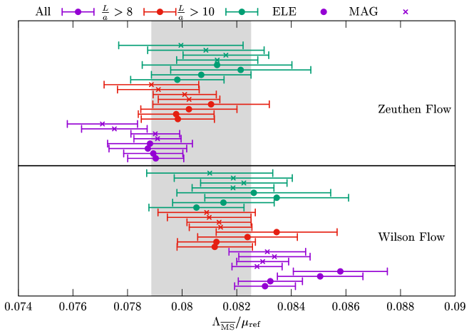
Figure 1: Landscape of the results for $\Lambda_{\overline{\rm MS}}/\mu_{\rm ref}$ given in table 3. The shaded region is our final result eq. (3.23). Once the coarser lattice $L/a=8$ is discarded, different analysis techniques give compatible results.

3.4.1 Comparison with perturbation theory

It is instructive to plot our results for the $\beta$-functions and compare them with their 3-loop perturbative predictions. This is illustrated in figure 2. It is clear from the figure that the GF based schemes show a very poor convergence to their expected perturbative behaviour. For the electric scheme, the non-perturbative data is barely compatible within errors with the 3-loop $\beta$-function at the most perturbative point, where $\alpha\sim 0.08$. The magnetic scheme shows even poorer convergence, with a clear deviation at $\alpha\sim 0.08$ between our data and the 3-loop prediction. In this case, looking even beyond the range covered by the data, our parametrization for the $\beta$-function appears to deviate from its 3-loop approximation down to couplings as small as $\alpha\sim 0.05$. With hindsight, these conclusions are not too surprising, given the large value of the $b_{2}$-coefficients in these schemes (cf. eq. (2.32)). The slightly better convergence of the electric scheme with respect to the magnetic one made us favour as our final result, eq. (3.23), a determination based on the electric rather than the magnetic coupling. Either way, however, a determination of the $\Lambda$-parameter based on the GF schemes is very much limited in the attainable precision due to these issues.

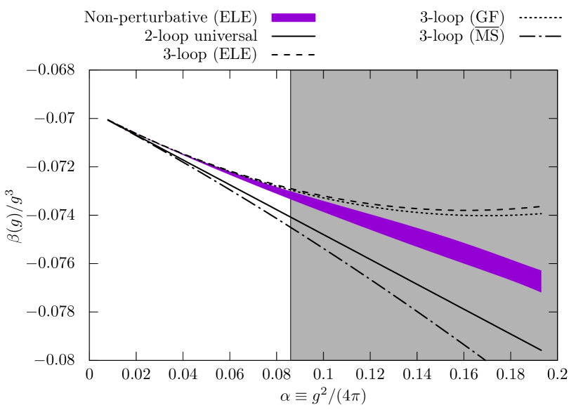
(a) Electric scheme.

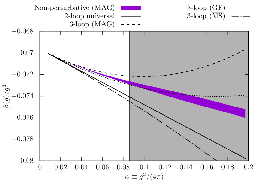
(b) Magnetic scheme

Figure 2: Comparison of the $\beta$-function in the electric/magnetic schemes with their perturbative predictions. We also show the perturbative predictions in the GF infinite volume and $\overline{\rm MS}$ schemes. The shaded region corresponds to the range where the data is available $\bar{g}^{2}\sim[1,2.5]$. See text for a discussion.

The effect of the poor convergence to perturbation theory of these schemes on the determination of $\Lambda_{\overline{\rm MS}}/\mu_{\rm ref}$ can be quantitatively studied by examining the dependence of $\Lambda_{\overline{\rm MS}}/\mu_{\rm ref}$ on the scale $\mu_{\rm PT}$ at which perturbation theory is used to extract it. More precisely, we can look at:

$$\phi_{\rm GF}(\alpha_{\rm PT})=\frac{\Lambda_{\overline{\rm MS}}}{\Lambda_{\rm GF}}\,\varphi_{\rm GF}^{(3)}(\bar{g}_{\rm GF,\,ref},\bar{g}_{\rm GF,\,PT})\mathrel{\mathop{=}\limits^{\vbox to3.01389pt{\kern-2.0pt\hbox{$\scriptstyle\mu_{\rm PT}\to\infty$}\vss}}}\frac{\Lambda_{\overline{\rm MS}}}{\mu_{\rm ref}}+\mathcal{O}(\alpha_{\rm PT}^{2})\,,\qquad\alpha_{\rm PT}\equiv\frac{\bar{g}^{2}_{\rm GF,\,PT}}{4\pi}\,,$$ (3.30)

where, as usual, $\bar{g}_{\rm GF,\,X}\equiv\bar{g}_{\rm GF}(\mu_{\rm X})$, and GF may refer to either the electric or the magnetic components of the GF coupling. The function $\varphi^{(3)}_{\rm GF}$ is defined by eq. (2.11) in terms of the GF $\beta$-function and its 3-loop perturbative approximation. As anticipated in the above equation, in the limit $\alpha_{\rm PT}\to 0$ the function $\phi_{\rm GF}$ approaches $\Lambda_{\overline{\rm MS}}/\mu_{\rm ref}$ with $\mathcal{O}(\alpha^{2}_{\rm PT})$ corrections. The latter are expected to be small if and only if 3-loop perturbation theory is a good approximation for the $\beta$-function at scales of $\mathcal{O}(\mu_{\rm PT})$. As stated above, however, this is not the case for the GF schemes, even at the largest energy scales we explored. At values of the couplings $\alpha_{\rm PT}=0.2$, for instance, where 3-loop perturbation theory is typically expected to be accurate, we find:

$$\frac{\phi_{\rm GF,\,e}(0.2)-\phi_{\rm GF,\,e}(0)}{\phi_{\rm GF,\,e}(0)}=\phantom{1}6.1(2.1)\%\,,\qquad\frac{\phi_{\rm GF,\,m}(0.2)-\phi_{\rm GF,\,m}(0)}{\phi_{\rm GF,\,m}(0)}=12.6(1.7)\%\,.$$ (3.31)

The approximations $\phi_{\rm GF,\,e}$, $\phi_{\rm GF,\,m}$ thus deviate from our final result eq. (3.23) by $\sim 6$% and 13%, respectively. These numbers are between 3 to 6 times larger than our uncertainty on eq. (3.23). Even at the largest energy scale reached by our simulations, where $\alpha_{\rm PT}\sim 0.08$, both schemes show a significant deviation from eq. (3.23) (cf. figure 3).

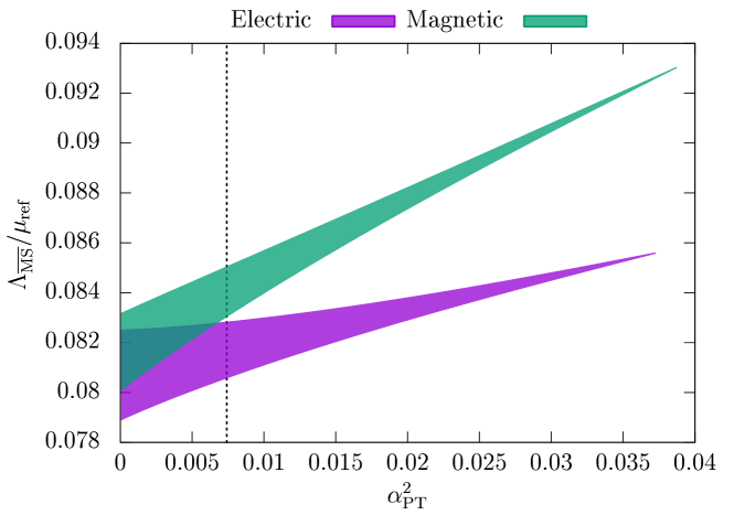
Figure 3: The ratio $\Lambda_{\overline{\rm MS}}/\mu_{\rm ref}$ estimated from the function $\phi_{\rm GF}(\alpha_{\rm PT})$ (see eq. (3.30)) as a function of the matching scale with perturbation theory (represented by $\alpha_{\rm PT}=\bar{g}^{2}_{\rm PT}/4\pi$). At $\alpha_{\rm PT}\sim 0.08$ (our most non-perturbative data point) the NNLO predictions using the electric and magnetic schemes disagree by $\sim 2.5\%$.

As anticipated, the issue of poor convergence has a dramatic effect on the precision that can be attained for $\Lambda_{\overline{\rm MS}}/\mu_{\rm ref}$ using GF based schemes. Due to the large corrections in eq. (3.30) one is forced to take as final estimate for $\Lambda_{\overline{\rm MS}}/\mu_{\rm ref}$ the value of $\phi_{\rm GF}(0)$, which requires an extrapolation. A competitive scheme, on the other hand, should allow us to quote as final result the estimate for $\Lambda_{\overline{\rm MS}}/\mu_{\rm ref}$ at, say, $\alpha\sim 0.1$, i.e. at the smallest couplings reached by our simulations (cf. Sect. 3.5). This clearly permits to reach a significantly higher precision. The result for,

$$\phi_{\rm GF,\,m}(0.1)=0.08492(85)\,,$$ (3.32)

for instance, has an error 50% smaller than eq. (3.23). Unfortunately, however, at this value of $\alpha$ the results in different schemes differ by a few standard deviations. These values are also significantly different from $\phi_{\rm GF}(0)$, indicating that a safe contact with perturbation theory has not been reached. In conclusion, using GF based schemes, 3-loop perturbation theory is not accurate enough to extract the $\Lambda$-parameter with $\sim 1\%$ error at $\alpha\sim 0.1$. The conclusions of this section are further corroborated by a more traditional step-scaling strategy to extract $\Lambda_{\overline{\rm MS}}/\mu_{\rm ref}$. We refer the interested reader to Appendix C for more details.

3.5 Non-perturbative matching to the SF scheme

Over the years the SF couplings have been widely employed in step-scaling studies [42, 9, 34, 56, 8], and recently their perturbative behaviour has been carefully investigated in the context of determining the $\Lambda$-parameter of QCD to a few per-cent accuracy. From these studies, we expect the matching of the SF schemes with perturbation theory to be quantitatively much better than what we observed above for the GF schemes. In particular, 3-loop perturbation theory may be precise enough for our purposes at scales where $\alpha\sim 0.1$. This in fact will be confirmed below.

Given these observations, in this section we consider a different strategy for determining $\Lambda_{\overline{\rm MS}}/\mu_{\rm ref}$. We will first match non-perturbatively the SF and the GF schemes, and then extract the $\Lambda$-parameter using perturbation theory in the SF schemes. To achieve this, we have measured the SF couplings on lattices of size $L/a=6,8,10,12,16$, and at values of the bare coupling $g_{0}$ that match our measurements of the GF couplings on $2L/a$ lattices, i.e. $L/a=12,16,20,24,32$, respectively. We thus combine a change of scheme with a change in the renormalization scale by a factor $s=2c$, where $c=0.3$ in our study. We collected from about $5\times 10^{5}$ measurements on the smaller lattices with $L/a=6$, up to $2\times 10^{6}$ measurements for $L/a=16$ (see table 17 for the exact figures). We measured both the SF coupling $\bar{g}^{2}_{\rm SF}$ and the observable $\bar{v}$, which gives us access to $\bar{g}^{2}_{{\rm SF},\nu}$ for any value of $\nu$ (cf. eq. (2.18)). In this section we focus exclusively on $\nu=0$. The consistency between determinations for different $\nu$-values is discussed in Appendix C.

With these results at hand, we fit the data for the GF and SF couplings as:

$$\frac{1}{\bar{g}^{2}_{\rm SF}(\mu)}-\frac{1}{\bar{g}^{2}_{\rm GF}(\mu/(2c))}=f(u)+\tilde{\rho}(u)\left(\frac{a}{L}\right)^{2}\,,\qquad(u=\bar{g}^{2}_{\rm GF}(\mu/(2c)))\,.$$ (3.33)

The function $\tilde{\rho}(u)$ parametrizes the cutoff effects in this relation by a simple polynomial:

$$\tilde{\rho}(u)=\sum_{k=0}^{n_{\tilde{\rho}}}\tilde{\rho}_{n}u^{n}\,.$$ (3.34)

We also use a polynomial for $f(u)$:

$$f(u)=\sum_{k=0}^{n_{f}}f_{n}u^{n}\,.$$ (3.35)

Using the perturbative relation, eq. (2.35), we could in principle fix the coefficients $f_{0},f_{1}$, to their perturbative values. Here, however, we refrain to do so. Clearly, this implies that the non-perturbative matching between the SF and GF schemes is only trustworthy within the available range of couplings i.e., for $\bar{g}_{\rm GF,\,SF}^{2}\sim 1-2$. We obtain good fits by taking, e.g., $n_{f}=2,3$ and $n_{\tilde{\rho}}=2$. We note however that our final results for $\Lambda_{\overline{\rm MS}}/\mu_{\rm ref}$ do not depend significantly on this particular choice. We only see some dependence if we include or not our coarser lattices (i.e. $L/a=6$ for the SF coupling and $L/a=12$ for the GF couplings). Any disagreement disappears once we perturbatively improve the SF data to 2-loop order in lattice perturbation theory (see appendix D). Having observed this, in order to be conservative, we prefer to discard the coarser lattice spacing for computing the matching, and use the 2-loop improved data. All our fits are then good with a $\chi^{2}/\text{dof}\sim 0.5-1$.

Once the function $f(u)$ has been determined, the $\beta$-function in the SF scheme can be inferred from the one in the GF scheme using the relation:

$$\mu\frac{{\rm d}{\bar{g}}_{\rm SF}(\mu)}{{\rm d}\mu}=\beta_{\rm SF}(\bar{g}_{\rm SF}(\mu))=\sqrt{1+uf(u)}\left[-\frac{f^{\prime}(u)-1/u^{2}}{(f(u)+1/u)^{2}}\right]\beta_{\rm GF}(\sqrt{u})\qquad(u=\bar{g}_{\rm GF}^{2}(\mu/(2c)))\,.$$ (3.36)

Note that since we are not interested in matching the GF schemes with their perturbative expressions, we can consider also fits for $\beta_{\rm GF}(g)$ where the $b_{2}$ coefficient is treated as a fit parameter, rather than being fixed to its perturbative value (cf. eq. (3.16)). In this case, the results for $\beta_{\rm SF}(g)$ only use as perturbative information the universal coefficients of the $\beta$-function, eq. (2.5). In particular the known value for $b_{2}^{\rm SF}$ is not used. We have determined $\beta_{\rm SF}$ using the data for $\beta_{\rm GF}$ both in the electric and magnetic GF scheme. The SF $\beta$-function determined this way is shown in figure 4(b). As one can see from the plot, as expected there is agreement between the determination from the electric and magnetic GF schemes. The non-perturbative data then match the perturbative prediction in all the range of couplings we covered.

(a) By using the non-perturbative matching between the SF and the GF schemes (eq. (3.33)), we can determine the $\Lambda_{\overline{\rm MS}}$ making contact with perturbation theory in the SF scheme. Due to the much better perturbative behavior (compare figure 2 and figure 4(b)), this strategy allows a more acurate and precise determination of $\Lambda_{\overline{\rm MS}}$.

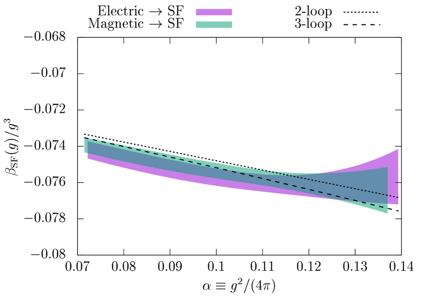
(b) The $\beta$-function in the SF scheme determined by matching non-perturbatively the SF and the GF schemes (see eq. (3.36)). In all the range of coupling our results agree with the perturbative 3-loop prediction. This contrast with the behaviour in the GF schemes (see figure 2).

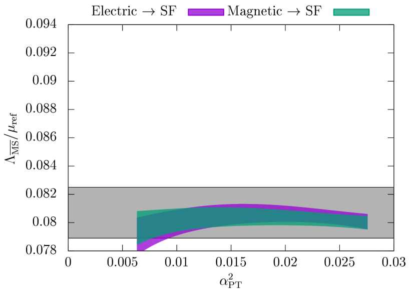
(c) The determination of $\Lambda_{\overline{\rm MS}}/\mu_{\rm ref}$ from the function $\phi_{\rm SF}(\alpha_{\rm PT})$ (see eq. (3.37)). The figure shows that the value of $\phi_{\rm PT}(\alpha_{\rm PT})$ is independent on $\alpha_{\rm PT}$, showing that the corrections $\mathcal{O}(\alpha_{\rm PT}^{2})$ are negligible within our statistical precision. This is in contrast with the behaviour in the GF schemes (see figure 3). The error band is the result of eq. (3.23).

Figure 4: The determination of $\Lambda_{\overline{\rm MS}}/\mu_{\rm ref}$ from a non-perturbative matching between the GF and SF schemes.

Similarly to what we did in the previous section for the GF coupling, we can now explore in the SF scheme the effect on $\Lambda_{\overline{\rm MS}}/\mu_{\rm ref}$ of matching with perturbation theory at different energy scales, $\mu_{\rm PT}$. To this end, we introduce the function ($\bar{g}_{\rm X,\,Y}\equiv\bar{g}_{\rm X}(\mu_{\rm Y})$):

$$\phi_{\rm SF}(\alpha_{\rm PT})=2c\frac{\Lambda_{\overline{\rm MS}}}{\Lambda_{\rm SF}}(b_{0}\bar{g}^{2}_{\rm GF,\,ref})^{\frac{-b_{1}}{2b_{0}^{2}}}{\rm e}^{-\frac{1}{2b_{0}\bar{g}^{2}_{\rm GF,\,ref}}}\times\\ \times\exp\big{\{}-I_{g}^{\rm GF}(\bar{g}_{\rm GF,\,ref},\bar{g}_{\rm GF,\,PT})-I_{g}^{\rm SF,3}(\bar{g}_{\rm SF,2c\mu_{\rm PT}},0)\big{\}},\quad\alpha_{\rm PT}\equiv\frac{\bar{g}^{2}_{\rm GF,\,PT}}{4\pi},$$ (3.37)

where $I_{g}^{\rm GF}$ is defined in terms of the non-perturbative $\beta$-function in either the electric or magnetic GF scheme (cf. eq. (2.6)), while $I_{g}^{\rm SF,3}$ integrates the perturbative 3-loop $\beta$-function in the SF scheme (cf. eq. (2.10)). This quantity is entirely analogous to eq. (3.30), the only difference being that once we arrive at the scale $\mu_{\rm PT}$ with the running in the GF scheme, we change to the SF scheme at the scale $2c\mu_{\rm PT}$, and we then use perturbation theory in the SF scheme (see figure 4(a) for a cartoon). Note that the factor $s=2c$ appearing on the r.h.s. of eq. (3.37) compensates the scale difference in matching the SF and GF schemes. The function $\phi_{\rm SF}$ has, of course, an asymptotic expansion of the form:

$$\phi_{\rm SF}(\alpha_{\rm PT})=\frac{\Lambda_{\overline{\rm MS}}}{\mu_{\rm ref}}+\mathcal{O}(\alpha_{\rm PT}^{2})\,,$$ (3.38)

in complete analogy with $\phi_{\rm GF}$. The crucial difference lies in the size of the $\mathcal{O}(\alpha_{\rm PT}^{2})$ corrections. As clearly shown in figure 4(c), in this case the corrections are negligible within our statistical precision. In contrast to the case of the GF schemes, the value of $\phi_{\rm SF}(\alpha_{\rm PT})$ is essentially independent on $\alpha_{\rm PT}$ in the range $\alpha_{\rm PT}\sim 0.1-0.2$. This allows us to take as our estimate for $\Lambda_{\overline{\rm MS}}/\mu_{\rm ref}$ the value of $\phi_{\rm SF}(\alpha_{\rm PT})$ at the smallest coupling reached in our simulations, which is: $\alpha_{\rm PT}=1.05/(4\pi)\sim 0.0836$. It is important to stress that this result does not rely on the 3-loop $\beta$-function coefficient $b_{2}$ of the GF schemes. Different fits to the GF $\beta$-function then give compatible results (see figure 5). In particular, the determinations show very good agreement once the coarser lattice, $L/a=8$, is dropped from the analysis of the GF $\beta$-function. Moreover, as already mentioned, changing the parametrization of the matching function $f(u)$ in eq. (3.33) results in insignificant changes in the final numbers.

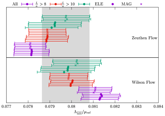
Figure 5: Results for the ratio $\Lambda_{\overline{\rm MS}}/\mu_{\rm ref}$ by quoting the value of $\phi_{\rm SF}(\alpha_{\rm PT})$ at the smaller value of the coupling $\alpha_{\rm PT}=1.05/(4\pi)\sim 0.0836...$. Different analysis correspond to different fits to the GF $\beta$-function as discussed in section 3.4.

As the final result of this strategy that combines the GF and SF couplings, we choose to quote the one based on the Zeuthen flow data for the magnetic GF scheme with $L/a>10$:

$$\frac{\Lambda_{\overline{\rm MS}}}{\mu_{\rm ref}}=0.0797(11)\qquad[1.37\%]\,.$$ (3.39)

This number has one of the largest uncertainties of all the analysis we considered, and its error covers all central values of the determinations which use only lattices with $L/a>8$. In conclusion, thanks to the better perturbative behaviour of the SF schemes, by non-perturbatively matching the GF and SF schemes we can reliably quote an uncertainty significantly smaller than in eq. (3.23). Similar conclusions are obtained using a more conventional step-scaling strategy based on the GF couplings, and considering different values of $\nu$ for the SF scheme. We refer the interested reader to Appendix C.

4 Connection to an hadronic scale

To compute the $\Lambda$-parameter in units of an hadronic quantity, like $t_{0}$ [11] or $r_{0}$ [28], we must relate this quantity with the technical scale $\mu_{\rm ref}$. In this section we consider two different strategies to compute this relation. Both rely on the determination of the $\beta$-function of the GF coupling at relatively low-energy scales. In the first strategy, we first use the $\beta$-function to relate $\mu_{\rm ref}$ with a convenient low-energy finite-volume scale, $\mu_{\rm had}$. We then relate, in a second step, this scale with the infinite volume scales $t_{0}$ and $r_{0}$. We shall refer to this strategy as "fixed scale determination". In the second strategy, instead, we use the knowledge of the $\beta$-function to match directly $\mu_{\rm ref}$ with $t_{0}$ and $r_{0}$; we shall refer to this as "global analysis".

4.1 The $\beta$-function at low-energy

We begin by defining two convenient low-energy finite-volume scales, one for each GF scheme. We do so through the conditions:

$$\bar{g}^{2}_{\rm GF,\,e}(\mu_{\rm had,e})=10.95=\bar{g}^{2}_{\rm GF,\,m}(\mu_{\rm had,m})\,;$$ (4.1)

note that $\mu_{\rm had,e}\neq\mu_{\rm had,m}$. The desired ratios of scales $\mu_{\rm ref}/\mu_{\rm had}$ can now be inferred once the $\beta$-function in the two schemes is known in the range of couplings: $\bar{g}^{2}\in[\bar{g}^{2}_{\rm GF,\,ref},\bar{g}^{2}_{\rm GF,\,had}]$. In this range, we find convenient to employ a parametrization of the $\beta$-function of the form:

$$\beta(x)=-\frac{x^{3}}{\sum_{k=0}^{n_{b}}p_{k}x^{2k}}\,.$$ (4.2)

This is completely analogous to eq. (3.28), the difference being that here we do not fix the coefficients $p_{0},p_{1},p_{2}$, to their perturbative values. As we saw for eq. (3.29), this parametrization allows us to express in a straightforward way the function $F$ of eq. (3.17) in terms of the parameters of the $\beta$-function, i.e.:

$$F(a,b)=H(a)-H(b),\qquad H(x)=\frac{p_{0}}{2x^{2}}-p_{1}\log x-\sum_{k=1}^{n_{b}-1}p_{k+1}\frac{x^{2k}}{2k}.$$ (4.3)

As done previously for the $\beta$-function at high-energy, the fit coefficients $p_{k}$ can then be determined by minimizing the $\chi^{2}$-function, eq. (3.18) (or eq. (3.26)); we again consider the parametrization (3.20) for the cutoff effects. Once $F$ is determined, the desired ratios of scales are given by:

$$\log\bigg{(}\frac{\mu_{\rm ref}}{\mu_{\rm had}}\bigg{)}=F(\bar{g}^{2}_{\rm GF,\,ref},\bar{g}^{2}_{\rm GF,\,had})\,.$$ (4.4)

We consider fits to data with $\bar{g}^{2}_{\rm GF}\in[2-4.7]$, and their corresponding SSFs. We obtain good fits choosing $n_{b}=2,3$, and we typically take $n_{c}=2,3$, although the final results are pretty much independent on the number of parameters used to parametrize the cutoff effects. Figure 6 collects a landscape of results. As one can see from the figure, we have excellent agreement between different analysis as long as we discard the coarser lattices with $L/a=8$. As our final results we quote:

$$\frac{\mu_{\rm ref}}{\mu_{\rm had,m}}=6.528(32)\quad[0.48\%]\,,\qquad\frac{\mu_{\rm ref}}{\mu_{\rm had,e}}=6.516(35)\quad[0.54\%]\,.$$ (4.5)

For completeness, we give below the fit coefficients and their covariance matrix, which describe the $\beta$-function in the electric scheme:

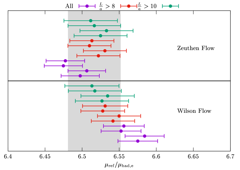
(a) $\mu_{\rm ref}/\mu_{\rm had,e}$

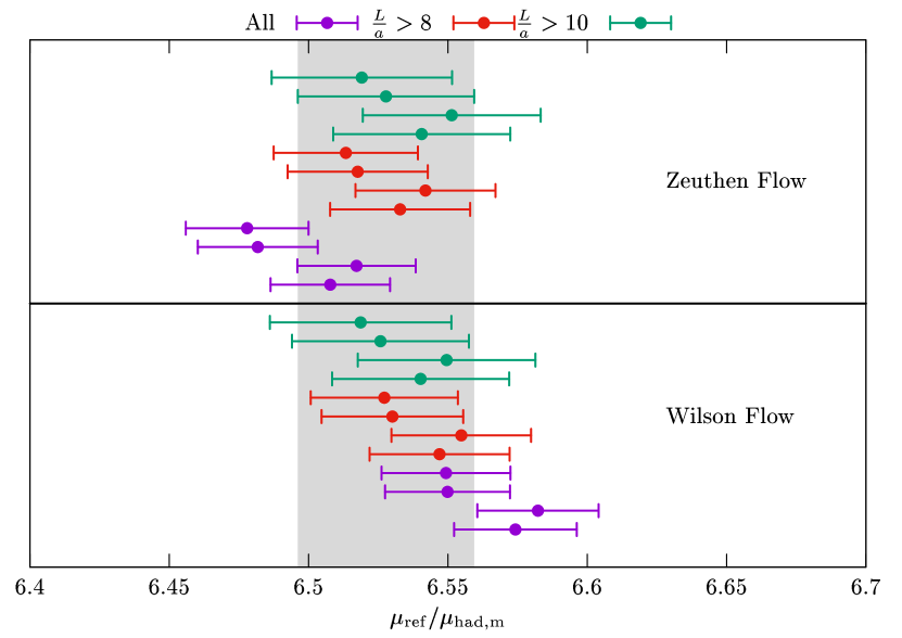
(b) $\mu_{\rm ref}/\mu_{\rm had,m}$

Figure 6: Results for the ratios $\mu_{\rm ref}/\mu_{\rm had,e}$ and $\mu_{\rm ref}/\mu_{\rm had,m}$. The different analysis correspond to different choices of discretization (labelled Zeuthen and Wilson), parametrizations of the $\beta$-function and cuts on the lattice resolutions (see text for more details).

$$p_{0}=14.86156402\,,\ p_{1}=1.03507289\,,\ p_{2}=-0.15702286\,,\ p_{3}=0.01250783\,,$$ (4.6)

$${\rm cov}(p_{i},p_{j})=\left(\begin{array}[]{cccc}7.19145589\times 10^{\text{-1}}&4.50192418\times 10^{\text{-1}}&-8.34709691\times 10^{\text{-2}}&4.60384717\times 10^{\text{-3}}\\ 4.50192418\times 10^{\text{-1}}&2.87728456\times 10^{\text{-1}}&-5.41797562\times 10^{\text{-2}}&3.02449220\times 10^{\text{-3}}\\ -8.34709691\times 10^{\text{-2}}&-5.41797562\times 10^{\text{-2}}&1.03377600\times 10^{\text{-2}}&-5.83491819\times 10^{\text{-4}}\\ 4.60384717\times 10^{\text{-3}}&3.02449220\times 10^{\text{-3}}&-5.83491819\times 10^{\text{-4}}&3.32558532\times 10^{\text{-5}}\\ \end{array}\right)\,.$$

$\beta$	$t_{0}/a^{2}$	$\beta$	$t_{0}/a^{2}$	$\beta$	$r_{0}/a$
5.9600	2.7854(62) †	6.4200	11.241(23) †	5.7000	2.9220(90) ††
5.9600	2.7875(53) ‡	6.4500	12.196(21) ‡	5.8000	3.6730(50) ††
6.0500	3.7834(47) ‡	6.5300	15.156(28) ‡	5.9500	4.898(12) ††
6.1000	4.4329(32) ⋆	6.6100	18.714(30) ‡	6.0700	6.033(17) ††
6.1300	4.8641(85) ‡	6.6720	21.924(81) ⋆	6.1000	6.345(13) ⋆
6.1700	5.489(14) †	6.6900	23.089(48) ‡	6.2000	7.380(26) ††
6.2100	6.219(13) ‡	6.7700	28.494(66) ‡	6.3400	9.029(77) ⋆
6.2900	7.785(14) ‡	6.8500	34.819(84) ‡	6.4000	9.740(50) ††
6.3400	9.002(31) ⋆	6.9000	39.41(15) ⋆	6.5700	12.380(70) ††
6.3400	9.034(29) ⋆	6.9300	42.82(11) ‡	6.5700	12.176(97)§
6.3700	9.755(19) ‡	7.0100	52.25(13) ‡	6.6720	14.103(92) ⋆
6.4200	11.202(21) ‡			6.6900	14.20(12)§
				6.8100	16.54(12)§
				6.9000	18.93(15) ⋆
				6.9200	19.13(15)§

Table 4: Results for $t_{0}/a^{2}$ and $r_{0}/a$ for different values of $\beta$. For the case of $t_{0}/a^{2}$ the relevant references are ^† [11], ^‡ [57], ^⋆ [58]. For $r_{0}/a$, instead, the results are from ^†† [59] and ^⋆ [58]. The data labeled ^§ is obtained from the values of $r_{c}/a$ of [60] together with $r_{c}/r_{0}=0.5133(24)$ which gives the quoted values of $r_{0}/a$.

4.2 Determination of $\sqrt{8t_{0}}\mu_{\rm ref}$: fixed renormalization scale

To obtain the sought-after relation $\sqrt{8t_{0}}\mu_{\rm ref}$ we now need to compute $\sqrt{8t_{0}}/a$ and $a\mu_{\rm had}$ for several values of the lattice spacing and extrapolate their product to the continuum limit, i.e.,

$$\lim_{a\to 0}\bigg{(}\frac{\sqrt{8t_{0}}}{a}\bigg{)}\times a\mu_{\rm had}=\sqrt{8t_{0}}\mu_{\rm had}\,.$$ (4.7)

This is done by determining the finite volume and hadronic scale in units of the lattice spacing at matching values of the bare coupling, $\beta=6/g_{0}^{2}$, which guarantees that the value of $a$ is the same up to scaling violations. The quantity $t_{0}/a^{2}$ is known from the literature over a wide range of $\beta$. In table 4 we collected the results used in our study and the corresponding references. Results for $t_{0}/a^{2}$ are known for values of the lattice spacing as fine as $0.025\,{\rm fm}$. Simulations at very fine lattice spacings deal with the problem of topology freezing [45] either by simulating very large physical volumes [57], or by using open boundary conditions in the Euclidean time direction [58].

In order to determine $a\mu_{\rm had}$, instead, for a given set of lattice sizes $L/a$, we must find the values of the bare coupling, $\beta=\beta_{\rm had}(L/a)$, for which the conditions (4.1) are satisfied. At these $\beta$’s we then have: $a\mu_{\rm had}=a/(cL)$ (cf. eqs. (2.29),(2.30)). Given our large set of data we can consider lattices with sizes $L/a\in[12,32]$. The values of $\beta_{\rm had}(L/a)$ are then easily found by performing interpolations of the data in $\beta$ at fixed $L/a$. The values of $\beta_{\rm had}(L/a)$ determined this way are collected in table 5, where the results for different lattice discretizations of the GF couplings are given.

From tables 4 and 5, it is clear that the values of $\beta$ for which the large volume quantities $t_{0}/a^{2}$ are available do not match exactly those which correspond to $\bar{g}_{\rm GF}^{2}(\mu_{\rm had})=10.95$ for our $L/a$’s. To obtain the products (4.7) at matching $\beta$-values we can thus proceed in either of the following two ways:

1. Given the results of table 4, we fit the data for $\log(t_{0}/a^{2})$ as a function of $g_{0}^{2}$. In practice, we obtain a good description of the data by using a simple polynomial fit of degree 5. In this way we can infer the values of $\log(t_{0}/a^{2})$ at the bare couplings of table 5, corresponding to the finite volume results for $a\mu_{\rm had}$.

2. We fit the results for $\beta_{\rm had}(L/a)$ as a function of $L/a$, or equivalently $a\mu_{\rm had}$. In this case, we obtain good fits using polynomials of degree 3. Given this functional form, we can then find the value of $a\mu_{\rm had}$ at the bare couplings where the large volume quantities $t_{0}/a^{2}$ have been computed (cf. table 4).

Figure 8 shows the continuum extrapolations of $t_{0}\mu_{\rm ref,m}^{2}$ determined according to the above strategies, and for different lattice discretizations for the GF couplings. For the case of the strategy 1 above we only use the data with $L/a>16$. The agreement among the different analysis techniques and the different discretizations is evident. We choose as final result the determination obtained following strategy 1 and based on the Zeuthen-flow data. This has the largest error and gives:

$$\sqrt{8t_{0}}\mu_{\rm had,m} =1.1961(35)\qquad[0.29\%]\,,\qquad\sqrt{8t_{0}}\mu_{\rm had,e} =1.1991(33)\qquad[0.27\%]\,.$$ (4.8)

Note the remarkable precision we obtain, i.e., around a 3 per-mille. Combining these results with those of eq. (4.5) we can quote

$$\sqrt{8t_{0}}\mu_{\rm ref}=7.808(46)\qquad[0.59\%]\,,$$ (4.9)

which uses the results for the magnetic scheme. The value obtained using $\mu_{\rm had,e}$ as intermediate scale instead is $\sqrt{8t_{0}}\mu_{\rm ref}=7.814(50)$, which is in good agreement.

			$\beta_{\rm had,\,e/m}(L/a)$
			Wilson Flow		Zeuthen Flow
$L/a$	$a\mu_{\rm had,e/m}$	$\bar{g}^{2}_{\rm GF,\,e/m}(\mu_{\rm had,e/m})$	Magnetic	Electric	Magnetic	Electric
32	0.1042	10.95	6.5609(17)	6.5588(18)	6.5617(17)	6.5598(19)
24	0.1389	10.95	6.3512(10)	6.3497(11)	6.35170(99)	6.3504(11)
20	0.1667	10.95	6.2209(14)	6.2191(16)	6.2219(14)	6.2204(15)
16	0.2083	10.95	6.0722(14)	6.0712(15)	6.0739(14)	6.0730(14)
12	0.2778	10.95	5.9004(16)	5.8992(17)	5.9033(16)	5.9023(16)

Table 5: Values of the bare coupling $\beta_{\rm had}(L/a)$ for different lattice sizes and discretizations which correspond to a fixed coupling $\bar{g}^{2}_{\rm GF}(\mu_{\rm had})=10.95$.

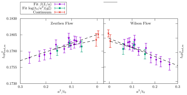
Figure 7: $t_{0}\mu_{\rm had,m}^{2}$.

Figure 8: Continuum extrapolations for $t_{0}\mu_{\rm had,m}^{2}$ using different strategies and discretizations for the GF couplings (see text for more details).

4.3 Determination of $\sqrt{8t_{0}}\mu_{\rm ref}$: global analysis

As can be seen from table 4, the flow scale in lattice units $t_{0}/a^{2}$ has been determined precisely even at very fine lattice spacings. This data, together with our results for the $\beta$-function at low energy in Sect. 4.1, calls for an alternative strategy to determine directly the product $\sqrt{8t_{0}}\mu_{\rm ref}$.

We start by performing once again a fit to the data for $\log(t_{0}/a^{2})$ of table 4 by a polynomial in $\beta=6/g_{0}^{2}$ of degree 5. This gives us a parametrization:

$$\log(t_{0}/a^{2})=P(g_{0}^{2})=\sum_{k=0}^{5}c_{k}g_{0}^{2k}\,,$$ (4.10)

in the range $\beta\in[5.96,7.01]$. We then consider our GF coupling data in the very same range of $\beta$, for lattice sizes $L/a=16,20,24,32,48$. For the ease of presentation we focus on the results for the magnetic components of the coupling; the analysis using the electric scheme gives compatible results. We will denote these generically as $u_{\rm FV}=\bar{g}^{2}_{\rm GF,m}(\mu_{\rm FV};a/L,g_{0})$. Using the parametrization of the $\beta$-function, eq. (4.2), valid in this range of couplings, we can compute the scale factor between the reference scale $\mu_{\rm ref}$ and the scale $\mu_{\rm FV}$ corresponding to a given coupling $u_{\rm FV}=\bar{g}_{\rm GF}^{2}(\mu_{\rm FV})$. This is simply given by (cf. eq. (4.3)):

$$\log\big{(}R(u_{\rm FV},a/L,g_{0}^{2})\big{)}=F(u_{\rm ref},u_{\rm FV})=\log\bigg{(}\frac{\mu_{\rm ref}}{\mu_{\rm FV}}\bigg{)}+\mathcal{O}(a^{2})\,,$$ (4.11)

where $u_{\rm ref}\equiv\bar{g}^{2}_{\rm GF}(\mu_{\rm ref})$, of eq. (3.14). Note that the scale factor associated to a given $u_{\rm FV}$ is only given up to discretization errors, the reason being that we are considering the value of the coupling at a certain $L/a$ and $g_{0}$. Given the results for $R$, we recall that $a\mu_{\rm FV}=a/(cL)$. The parametrization (4.10) then allows us to determine the second matching factor:

$$Q(u_{\rm FV},a/L,g_{0}^{2})=\sqrt{8}\exp\left(\frac{P(g_{0}^{2})}{2}\right)\times\bigg{(}\frac{a}{cL}\bigg{)}=\sqrt{8t_{0}}\mu_{\rm FV}+\mathcal{O}(a^{2})\,,$$ (4.12)

which relates the given finite-volume scale $a\mu_{\rm FV}$ with our hadronic quantity in lattice units.

Figure 9: The product $S_{t_{0}}$ of the running factor $R$ and the matching factor $Q$ (see eq. (4.13)). This has to be constant and equal to $\sqrt{8t_{0}}\mu_{\rm ref}$ up to discretization errors. The plot shows that these are very small. The error band shows the result of the fit, eq. (4.15).

Combining finally the factor $R$ of eq. (4.11) with $Q$ of (4.12) we obtain:

$$S_{t_{0}}(u_{\rm FV},a/L,g_{0}^{2})=R(u_{\rm FV},a/L,g_{0}^{2})\times Q(u_{\rm FV},a/L,g_{0}^{2})=\sqrt{8t_{0}}\mu_{\rm ref}+\mathcal{O}(a^{2})\,,$$ (4.13)

which, up to discretization errors, is the product $\sqrt{8t_{0}}\mu_{\rm ref}$ we were after. Note that by construction the dependence on $u_{\rm FV}$ cancels in the leading term of the product, eq. (4.13): only discretization errors thus depend on $u_{\rm FV}$. The latter turn out to be relatively small. This can be appreciated in figure 9, which shows the different results for the factor $S_{t_{0}}$. As we can see from the figure, the product $S_{t_{0}}$ is approximately constant as a function of $u_{\rm FV}$ with variations of at most 2% when changing $u_{\rm FV}\sim[3.5,11.5]$. This observation suggests to fit our results for $S_{t_{0}}(u_{\rm FV},a/L,g_{0}^{2})$ as:

$$S_{t_{0}}(u_{\rm FV},a/L,g_{0}^{2})=a_{0}+\sum_{k=1}^{n_{c}}\rho_{k}u_{\rm FV}^{k}\Big{(}\frac{a}{L}\Big{)}^{2}\,,$$ (4.14)

where $a_{0}$ and $\rho_{k}$ are fitting parameters. The continuum result $\sqrt{8t_{0}}\mu_{\rm ref}$, corresponding to the coefficient $a_{0}$ of the fit, shows very little dependence on the degree of the polynomial describing the cutoff effects, as long as $n_{c}>1$. As our final estimate we quote:

$$\sqrt{8t_{0}}\mu_{\rm ref}=7.809(37)\qquad[0.5\%]\,,$$ (4.15)

which is based on the Zeuthen-flow data in the magnetic scheme for $L/a\geq 16$ and uses $n_{c}=2$. This result is in agreement with our previous result, eq. (4.9). We note that including also lattices with $L/a<16$ gives completely compatible results with eq. (4.15), but with smaller uncertainties.

4.4 Determination of $r_{0}\mu_{\rm had}$

The strategies we used to compute $\sqrt{8t_{0}}\mu_{\rm had}$ can also be applied for the determination of $r_{0}\mu_{\rm had}$. In this case, however, the situation is a little complicated by a few technical issues. First of all, the different results for $r_{0}/a$ available in the literature which we could consider [58, 60, 59] use different discretizations for the relevant observables. Secondly, two of these determinations, refs. [60, 59], are more than 20 years old. A note of concern in this case is thus the issue of topology freezing [45], which was not known at the time of these computations. This issue is potentially more significant at the very fine lattice spacings simulated in ref. [60], while the results of ref. [59] are confined to substantially larger spacings. The more recent determination of $r_{0}/a$ in [58], on the other hand, employs open boundary conditions. In addition, their values for $r_{0}/a$ cover a factor two in lattice spacings and reach down to small spacings comparable to those of [60] (cf. table 4). For these reasons we consider safer to restrict our attention in the following only to the results of [58, 59].

Most of the results of [58] have been obtained at values of the bare coupling $g_{0}^{2}$ which lie outside the range of bare couplings of table 5 (cf. table 4 where the results of [58] are labelled with a $\star$). This means that the fixed scale strategy considered in Sect. 4.2 cannot really be applied to this data set. A fixed scale determination can only be considered for the results of [59] (which are labelled by ^†† in table 4). For these we opt for strategy 2 of Section 4.2. We thus use the same fit for $\beta_{\rm had}(L/a)$ as a function of $L/a$ considered there, which is based on a 3rd degree polynomial. Given this functional form, we then find the value of $a\mu_{\rm had}=a/(cL)$ at the values of $g_{0}^{2}$ where $r_{0}/a$ is known, and compute $r_{0}\mu_{\rm had}$. The continuum extrapolation

$$\qquad\lim_{a\to 0}\bigg{(}\frac{{r_{0}}}{a}\bigg{)}\times a\mu_{\rm had}={r_{0}}\mu_{\rm had}\,,$$ (4.16)

corresponding to the $r_{0}/a$ data of ref. [59] are shown in figure 10. Using the results of these extrapolations and those of eq. (4.5) we find:

4-point extrapolation: $$r_{0}\mu_{\rm ref}=8.327(58)\qquad[0.70\%]\,,$$ (4.17)

3-point extrapolation: $$r_{0}\mu_{\rm ref}=8.277(75)\qquad[0.90\%]\,.$$ (4.18)

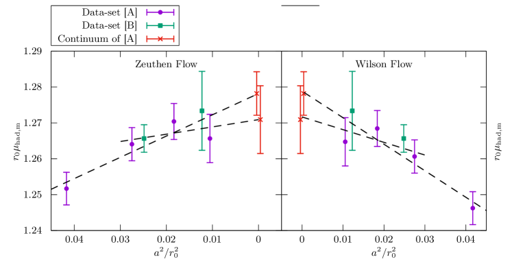
Figure 10: Continuum extrapolations of $r_{0}\mu_{\rm had,m}$ using the data set [A] [59] and the results of table 5. For illustration, the two points of data set [B] [58] in the range of $\beta$ covered by the finite volume simulations (table 5) are also plotted. These however are not used for any continuum extrapolation (see main text for the details).

The global approach described in Section 4.3 can on the other hand also be used for the $r_{0}/a$ data of ref. [58]. We thus begin by fitting the data for $r_{0}/a$ as a function of the bare coupling $g_{0}^{2}$. We do this separately for the data set of [58] (labelled [B] in figure 11) and for the data set of [59] previously used (labelled [A] in figure 11); this because the two computations use different observable discretizations. With these functional forms at hand, we then determine the product of the running factor $\mu_{\rm ref}/\mu_{\rm FV}$ (cf. eq. (4.11)) and the matching factor $r_{0}\mu_{\rm FV}$ (cf. eq. (4.12)). The result:

$$S_{r_{0}}(u_{\rm FV},a/L,g_{0}^{2})=r_{0}\mu_{\rm ref}+\mathcal{O}(a^{2})\,,$$ (4.19)

is expected to be constant, up to scaling violations. Figure 11 shows the quantity $S_{r_{0}}$ for the two data sets. It is clear that scaling violations within each data set are very small. Looking at the continuum extrapolated values, obtained after fitting separately the two data sets to a constant with cutoff effects parametrized by a 1st degree polynomial (cf. eq. (4.14)), we find:

Data set [A]: $$r_{0}\mu_{\rm ref}=8.294(62)\,,$$ (4.20)

Data set [B]: $$r_{0}\mu_{\rm ref}=8.297(64)\,.$$ (4.21)

which are in very good agreement.

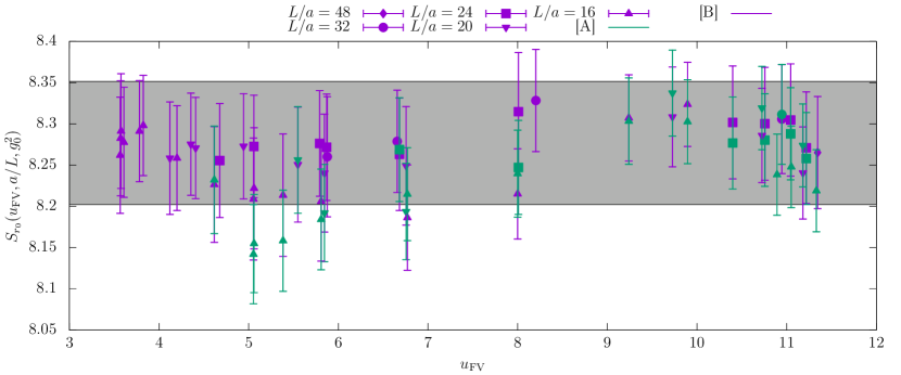
Figure 11: The product $S_{r_{0}}(u_{\rm FV},a/L,g_{0}^{2})$ of the running factor $R$ and the matching factor $Q_{r_{0}}$ (analogous to eq. (4.12) for $r_{0}$). This has to be constant and equal to $r_{0}\mu_{\rm ref}$ up to discretization errors; the plot clearly shows that these are very small for both data sets. In different colours we have the two data sets: [A] is ref [59], [B] is ref [58] (cf. table 4), while different symbols correspond to different lattice sizes. The grey error band is the result of eq. (4.18) (see main text for more details).

To conclude with the determination of $r_{0}\mu_{\rm ref}$, a conservative option for us is to quote the result of the 3-point extrapolation, eq. (4.18). Among the consistent analysis that we showed, this gives the result with the largest uncertainty.

5 The $\Lambda$-parameter

We are now ready to express $\Lambda_{\overline{\rm MS}}$ in terms of the hadronic scales $t_{0}$ and $r_{0}$. Our first main result is:

$$\sqrt{8t_{0}}\,\Lambda_{\overline{\rm MS}}=\frac{\Lambda_{\overline{\rm MS}}}{\mu_{\rm ref}}\times\frac{\mu_{\rm ref}}{\mu_{\rm had,m}}\times\sqrt{8t_{0}}\mu_{\rm had,m}=0.6227(98)\qquad[1.57\%]\,.$$ (5.1)

The first factor on the r.h.s. of this equation comes from the non-perturbative high-energy determination of the GF $\beta$-function in the electric scheme, combined with a non-perturbative matching of the GF and SF schemes. Thanks to this strategy, perturbation theory in the SF scheme could be safely used to run to infinite energy and obtain the result of eq. (3.39). The second factor derives instead from our determination of the $\beta$-function at low-energies in the magnetic GF scheme (cf. eq. (4.5)). The third and last factor is the non-perturbative matching of the magnetic GF coupling with the gradient flow scale $t_{0}$, eq. (4.8). The result in eq. (5.1) would not practically change, if we were to choose the scale $\mu_{\rm had,e}$ defined in the electric scheme in the second and third factor. We would also obtain a perfectly compatible result ($\sqrt{8t_{0}}\,\Lambda_{\overline{\rm MS}}=0.6227(94)$), if we replaced the last two factors with $\sqrt{8t_{0}}\mu_{\rm ref}$ determined via the global approach, eq. (4.15).

Our final error estimate ($\sim 1.6\%$) is very conservative. All three factors are determined by dropping the two coarsest lattice spacings at our disposal, and we typically chose as final result the analysis with the largest uncertainty. The only exception was when we favoured the result of eq. (3.39) over eq. (3.23). We found however compelling to match with the asymptotic perturbative regime in the SF rather than the GF scheme. Using the GF scheme would have indeed increased our final error by more than 50%, due to the bad convergence of its perturbation theory; this despite of the fact that we had access to the non-perturbative running of the coupling up to very large energy scales, where $\bar{g}_{\rm GF}^{2}\sim 1$.

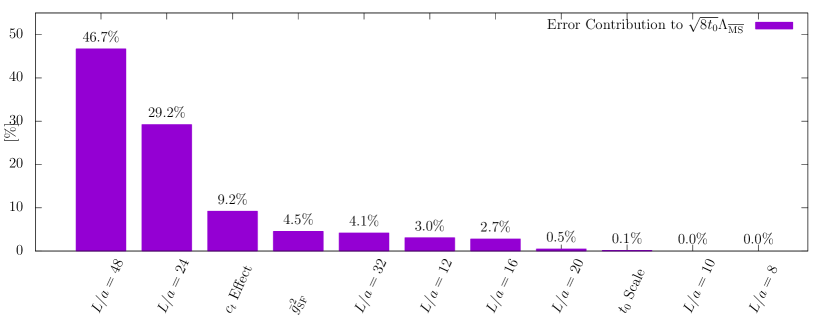
Figure 12: Separate contributions to the square error of $\sqrt{8t_{0}}\,\Lambda_{\overline{\rm MS}}$, eq. (5.1). Most of the error comes from the simulations on the largest lattices. The effect of the systematic uncertainty associated with $\mathcal{O}(a)$ terms (labelled $c_{t}$ effect) is only a small fraction of the error. Also the simulations that determined the SF coupling (labelled $\bar{g}^{2}_{\rm SF}$), give a small contribution to the error.

Looking at the different contributions to our final uncertainty, it is clear from eq. (3.39) that most of the uncertainty comes from the determination of the non-perturbative running from $\alpha=0.2$ to $\alpha\sim 0.08$. Given the high-precision we aimed for, however, we found compulsory to reach, non-perturbatively, these high-energy scales, and accurately test the applicability of perturbation theory. Figure 12 then illustrates the separate contribution to the total error squared from the different simulations and some other sources. Most of our error comes from the most expensive simulations, while for instance the contribution from the uncertainty on $t_{0}$ is completely negligible. Also the systematic uncertainty deriving from our ignorance of the boundary $\mathcal{O}(a)$ counterterm (labelled as "$c_{t}$ effect" in the figure) contributes only little to the final uncertainty. Moreover, in our strategy the SF coupling is only used at very high energies, where it is measured very precisely and with negligible cutoff effects. Consequently, its contribution to the final error is very small. In summary, our final uncertainty is completely dominated by the statistical uncertainty in the measurements of the GF coupling on our finest/largest lattices. The results could thus be improved significantly by just investing more computer time on these simulations.

A completely analogous analysis leads to:

$$r_{0}\,\Lambda_{\overline{\rm MS}}=0.660(11)\qquad[1.7\%]\,,$$ (5.2)

where we have used the result for $r_{0}\mu_{\rm ref}$ based on the 3-point extrapolation of data set [A], eq. (4.18).

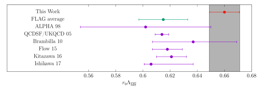
Figure 13: Comparison of our results for $r_{0}\Lambda_{\overline{\rm MS}}$ with results from the literature. For comparison we include all results that pass the FLAG criteria and thus enter their final average [61]. These are: ALPHA 98 [62], QCDSF/UKQCD 05 [63], Brambilla [64], Flow 15 [65], Kitazawa 16 [66], Ishikawa 17 [67].

Figure 13 shows a comparison of our computations with some other determinations available in the literature. More precisely, we have included the results entering the last FLAG average [61]. We find a significant discrepancy with some of these determinations, in particular with those of QCDSF/UKQCD 05 [63], Flow 15 [65] and Kitazawa 16 [66]. These determinations extract the $\Lambda$-parameter from measurements of Wilson loops, and rely on 2-loop bare lattice perturbation theory at a scale of a few GeVs. Here we recall that our final results use continuum extrapolations performed with data that cover a factor two in lattice spacings, with two extra lattice spacings (reaching a factor 3 change in $a$) used to check the consistency of our results. The non-perturbative running is performed up to very high energy scales where $\alpha<0.1$, and our matching with perturbation theory has been performed in several renormalization schemes. Our determination satisfies the most stringent of the FLAG criteria. Nevertheless there is a significant discrepancy with the FLAG average. Although we think that the FLAG criteria are conservative, this work shows that even computations that meet these criteria can differ by more than the quoted uncertainties. This discrepancies need further investigation, and once clarified the criteria used to rate different lattice determinations of the strong coupling might need to be readjusted. Also the authors believe that given the level of precision reached by current computations, one should probably consider $\sqrt{8t_{0}}\Lambda_{\overline{\rm MS}}$ rather than $r_{0}\Lambda_{\overline{\rm MS}}$ as the standard quantity of comparison.

6 Conclusions

Renormalization schemes based on the gradient flow have many attractive properties for applications in lattice QCD. Renormalized couplings are defined via observables with very small variance, which allows to attain great statistical precision. In addition, the coupling is given directly by an expectation value. Hence, there are no systematic errors associated with extracting properties from the large Euclidean time behaviour of a correlator. By using a renormalization scheme based on the gradient flow we have obtained a rather precise determination of the $\Lambda$-parameter in the $SU(3)$ gauge theory. Along the way we have learned several important lessons that will come useful when applying this technology to the more relevant case of QCD.

Using finite size scaling techniques we have determined non-perturbatively the $\beta$-function in a range of couplings $\alpha\sim 0.1-1$. Our results indicate that at energy scales where $\alpha\sim 0.1$ contact with 3-loop perturbation theory is not safe for GF schemes if one aims at a precision $\sim 0.5\%$ in $\alpha_{s}$.

One might argue that our particular setup (finite volume renormalization schemes with Schrödinger functional boundary conditions in the pure gauge theory), can cast some doubts on the general validity of our conclusions. In this respect one should first note that we have checked two different renormalization schemes (based on the electric and magnetic components of the energy density at positive flow time, respectively). The scheme based on the electric components, in particular, has a very similar perturbative behaviour to the corresponding infinite volume scheme (i.e. their non-universal 3-loop coefficients of the $\beta$-function are pretty close; see e.g. figure 2(a)). Secondly, if one considers the parametric uncertainty originating from the missing perturbative orders in extracting $\alpha_{s}$ from the infinite-volume GF coupling in QCD one reaches similar conclusions to our non-perturbative study: the extraction of $\alpha_{s}$ at the electroweak scale in the GF scheme carries a 0.5% theoretical uncertainty. If the extraction is performed at a few GeV (the energy scale typically accessible to large volume simulations), the theoretical uncertainty increases to $\sim 2-3\%$. Quark effects are absent in our study, but perturbatively their effect at high energy is small compared to the effect of the gluons [17]. The presence of quarks is thus expected not to change the picture very much. We conclude that the qualitative conclusions of our study are indeed general.

Our work allows us to precisely determine the pure gauge $\Lambda$-parameter in units of a typical hadronic scale (we considered both $t_{0}$ and $r_{0}$). Our result for $r_{0}\Lambda_{\overline{\rm MS}}$, with a precision $\sim 1.7\%$, shows some tension with other recent lattice computations, in particular with those where the $\overline{\rm MS}$-coupling is extracted from Wilson loops at an energy scale set by the lattice cutoff. One drawback of the GF couplings are the relatively large cutoff effects, which have been observed in many different applications (see [15] for an overview). Despite the fact that we have a solid theoretical understanding of the nature of these cutoff effects [16], they are still the main source of concern when considering GF-based observables. In order to have discretization effects under control we used 5 different lattice resolutions which cover a factor 3 in the spacing, and two different discretizations to integrate the flow equations and compute our observables. We see no deviation from pure $\mathcal{O}(a^{2})$ scaling violations. Despite these observations, we quote results where the two coarsest lattice spacings are discarded, and we add a generous estimate for the $\mathcal{O}(a)$ boundary effects. We recall that we have performed the running non-perturbatively up to very large energy scales, we have matched with the perturbative behaviour in four different renormalization schemes (with their respective $\Lambda$-parameters varying by factors of two), and used at least two different methods to match with a large volume hadronic scale. All in all, the significant discrepancy with the results in the literature shows the difficulty in extracting the fundamental parameters of the Standard Model with high precision.

We conclude by pointing out that the results of this work represent a serious warning for any attempt of reducing the current uncertainty of the world average value of $\alpha_{s}$ using lattice QCD and the GF schemes, especially if one aims at an infinite volume determination. Here the range of scales that can be explored is limited to $\alpha\gtrsim 0.25$, completely insufficient to quote sub-percent precision in $\alpha_{s}$. On the positive side we have shown a viable strategy to reach a precision of $0.3\%$ in $\alpha_{s}$. It combines the use of the GF schemes to determine the running non-perturbatively, and a non-perturbative matching at high-energy with the traditional SF schemes, that show small effects in the truncation of the perturbative series. Such a project would also require a precise and accurate determination of the hadronic scale in a theory with three or more active quarks [68].

Appendix A Continuum limit of GF couplings

Several studies have shown that renormalized couplings defined through the gradient flow are affected by significant cutoff effects (see e.g. ref. [15] and references therein). These cutoff effects have been first carefully studied at tree-level of perturbation theory [69], and later more systematically in the context of Symanzik’ effective theory [16]. Despite these efforts, however, they remain the main source of concern in applications of running couplings derived from the gradient flow.

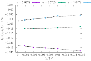
(a) Continuum extrapolations of the lattice SSF of the magnetic GF coupling at 3 target values of the coupling, eq. (A.1). (Data from table 6.) We consider the lattice resolutions: $L/a=8,10,12,16,24$, and perform linear fits of the data in $(a/L)^{2}$, with and without the coarsest lattice, $L/a=8$.

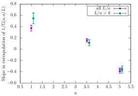
(b) Slopes $\tilde{\rho}$ of the continuum extrapolations of $1/\Sigma_{2}$ (cf. eq. (A.2)). (Data from table 6.) As we can see, the slope is positive at weak couplings, while turns negative at strong couplings.

In order to establish that the lattice resolutions employed in our study are fine enough to obtain accurate continuum extrapolations, we here analyse in detail the continuum extrapolation of the lattice step scaling function, $\Sigma_{2}(u,a/L)$, for the magnetic GF scheme, at 3 representative values of the coupling; these are:

$$u_{1}=1.04784,\qquad u_{2}=3.5705,\qquad u_{3}=5.0578\,.$$ (A.1)

Note that we shall focus on our preferred choice of discretization for the observable, i.e., Zeuthen flow/improved definition (cf. Sect. 3.1). To perform the continuum limit of the lattice SSF at these coupling values, we first need to find the values of the bare coupling $\beta$ for the chosen lattice sizes, for which the renormalized coupling, $u=\bar{g}^{2}_{\rm GF,\,m}(\mu)$, is equal to the target values (A.1). We did this for lattice sizes: $L/a=8,10,12,16,24$. The results of this tuning are given in the third and fourth columns of table 6. Once the values of the bare coupling are determined, at these $\beta$-values we compute the GF coupling on lattices of double size, i.e. with $L/a=16,20,24,32,48$, respectively. The corresponding results are given in the last column of table 6. Finally, the lattice SSFs so obtained can be extrapolated to the continuum limit (see figure 14(a)).

$u$	$L/a$	$\beta$	$\bar{g}^{2}_{\rm GF\,m}(\mu)$	$\bar{g}^{2}_{\rm GF\,m}(\mu/2)$
$u_{1}$	8	10.1106	1.04784(18)	1.16469(62)
	10	10.2830	1.04784(29)	1.16540(63)
	12	10.4258	1.04784(26)	1.16851(64)
	16	10.6586	1.04784(24)	1.17030(76)
	24	11.0000	1.04784(54)	1.17157(68)
	$\infty$ (Fit $1/\Sigma_{2}$; All $L/a$)		1.04784	1.17195(70)
	$\infty$ (Fit $\phantom{1/}\Sigma_{2}$; All $L/a$)		1.04784	1.17195(69)
	$\infty$ (Fit $1/\Sigma_{2}$; $L/a>8$)		1.04784	1.17325(91)
	$\infty$ (Fit $\phantom{1/}\Sigma_{2}$; $L/a>8$)		1.04784	1.17322(86)
$u_{2}$	8	6.3598	3.5705(24)	5.808(8)
	10	6.5197	3.5705(13)	5.844(8)
	12	6.6559	3.5705(18)	5.869(9)
	16	6.8786	3.5705(17)	5.876(13)
	24	7.2000	3.5705(31)	5.871(13)
	$\infty$ (Fit $1/\Sigma_{2}$; All $L/a$)		3.5705	5.897(12)
	$\infty$ (Fit $\phantom{1/}\Sigma_{2}$; All $L/a$)		3.5705	5.896(11)
	$\infty$ (Fit $1/\Sigma_{2}$; $L/a>8$)		3.5705	5.888(15)
	$\infty$ (Fit $\phantom{1/}\Sigma_{2}$; $L/a>8$)		3.5705	5.888(13)
$u_{3}$	8	5.9900	5.0578(21)	15.555(61)
	10	6.1365	5.0578(24)	15.037(59)
	12	6.2654	5.0578(26)	14.839(59)
	16	6.4742	5.0578(26)	14.686(70)
	24	6.7859	5.0578(61)	14.353(77)
	$\infty$ (Fit $1/\Sigma_{2}$; All $L/a$)		5.0578	14.303(58)
	$\infty$ (Fit $\phantom{1/}\Sigma_{2}$; All $L/a$)		5.0578	14.278(60)
	$\infty$ (Fit $1/\Sigma_{2}$; $L/a>8$)		5.0578	14.317(75)
	$\infty$ (Fit $\phantom{1/}\Sigma_{2}$; $L/a>8$)		5.0578	14.304(74)

Table 6: Data for the lattice step scaling function, $\Sigma_{2}(u,a/L)$, of the magnetic GF coupling, at the target couplings of eq. (A.1). The results of different continuum extrapolations are given.

We consider for $\Sigma_{2}$ continuum extrapolations linear in $(a/L)^{2}$. Moreover, in order to gain some insight on higher-order discretization errors we consider linear extrapolations in $(a/L)^{2}$ of $1/\Sigma_{2}$. We expect these two strategies to give compatible results up to $\mathcal{O}((a/L)^{4})$ errors. We thus have:

$$\Sigma_{2}(u,a/L)=\sigma_{2}(u)+\rho\left(\frac{a}{L}\right)^{2}\,,\qquad\frac{1}{\Sigma_{2}(u,a/L)}=\frac{1}{\sigma_{2}(u)}+\tilde{\rho}\left(\frac{a}{L}\right)^{2}\,.$$ (A.2)

As a further test on the scaling properties of our data, we also study the effect of discarding our coarser lattice with $L/a=8$ from the extrapolations.

Having this noticed, all our fits have good quality, and the agreement among different determinations of the continuum SSF, $\sigma_{2}(u)$, is in fact quite good (compare the rows marked by $L/a=\infty$ in table 6). We thus conclude that for our choice of discretization, our data show no significant deviation from $\mathcal{O}(a^{2})$ scaling. In addition, figure 14(a) shows that the slope of the continuum extrapolations is positive at weak couplings, while changes to negative at strong couplings. Somewhere around $u\sim 4$, the data have no significant cutoff effects.

In summary, the detailed study presented in this appendix shows that once lattice sizes in the range $L/a=8-24$ are considered, within the whole range of couplings $u\in[1,5]$ the continuum extrapolations of the lattice step scaling function of the GF coupling present no significant deviation from $\mathcal{O}(a^{2})$ scaling within our precision.

Appendix B Boundary $\mathcal{O}(a)$ effects

It is well-known that due to the breaking of translational invariance in the time direction, even the pure Yang-Mills theory with Schrödinger functional boundary conditions suffers from $\mathcal{O}(a)$ discretizations effects [6]. These can in principle be entirely removed by a proper tuning of a single boundary counterterm coefficient, $c_{t}(g_{0})$ (cf. eq. (3.1)). Unfortunately, however, in practice there is no compelling method to determine $c_{t}$ non-perturbatively. As a result, at present, given our choice of Wilson gauge action, $c_{t}$ is only known in perturbation theory to two-loop order [32, 33]. The leading discretization errors in our data are thus parametrically of $\mathcal{O}(g_{0}^{6}a/L)$. On the other hand, the results of the investigation in Appendix A, where we ignored any $\mathcal{O}(a)$ effects in the data, support the conclusion that these effects are in practice very small, and below our statistical precision. Nonetheless, in order to guarantee the high-precision of our results, we here want to address this potential source of systematic effects in detail. To this end, we measured the GF couplings for several values of $c_{t}$ which are shifted from the 2-loop result, $c_{t}^{\star}$, used in the simulations:

$$c_{t}^{\star}(g_{0})=1-0.08900\times g_{0}^{2}-0.0294\times g_{0}^{4}\qquad(g^{2}_{0}=6/\beta)\,.$$ (B.1)

We did this for $L/a=8,10,12$, and at the $\beta$-values corresponding to the 3 couplings of eq. (A.1). The results we obtained are collected in table 7. The deviation, $\Delta\bar{g}^{2}_{\rm GF,\,e/m}$, of these results from the couplings of eq. (A.1), is a clear measure of the sensitivity of the coupling on the boundary improvement coefficient $c_{t}$. The data of table 7 is well represented by a fit:

$$\bar{g}^{2}_{{\rm GF},\,c_{t}^{\star}+\Delta c_{t}}=\bar{g}^{2}_{{\rm GF},\,c_{t}^{\star}}+\frac{a}{L}\left(a_{0}\bar{g}^{2}_{{\rm GF},\,c_{t}^{\star}}+a_{1}\bar{g}^{4}_{{\rm GF},\,c_{t}^{\star}}\right)\Delta c_{t}\,,$$ (B.2)

where $\bar{g}^{2}_{{\rm GF},\,c_{t}}$ is the GF coupling (either electric or magnetic) measured for a given $c_{t}$, and $\Delta c_{t}=c_{t}-c_{t}^{\star}$. For the fit coefficients $a_{0},a_{1}$ we obtain the results:

$$\bar{g}^{2}_{\rm GF,\,m}:\qquad a_{0}=-0.14(5)\,, \quad a_{1}=-0.26(3)\,.$$ (B.3a)

$$\bar{g}^{2}_{\rm GF,\,e}:\qquad a_{0}=-0.48(5)\,, \quad a_{1}=-0.25(3)\,.$$ (B.3b)

As expected from general considerations, the electric components are the most affected by boundary $\mathcal{O}(a)$ effects [15]. The values of these fit coefficients, on the other hand, are basically the same for our two choices of discretization of the observable, i.e., Wilson flow/clover and Zeuthen flow/improved observable.

Having established the sensitivity of the GF couplings around the two-loop value of $c_{t}$, eq. (B.1), in order to estimate the uncertainty to attribute to our data for the incomplete tuning of $c_{t}$, we now need an estimate for the difference between $c_{t}^{\star}$ and the non-perturbative value of $c_{t}$. Having no information about the latter, a reasonable guess is to take for this deviation the full two-loop term of the series eq. (B.1). Given the fact that the coefficients of the series (B.1) appear to decrease with the order, our estimate can be considered a conservative one.

In conclusions, we add in quadrature to the statistical uncertainty of the GF couplings computed at $c_{t}=c_{t}^{\star}$ and for a given $g_{0}$ and $L/a$, the systematic uncertainty:

$$\delta_{c_{t}}\bar{g}^{2}_{\rm GF}=\frac{a}{L}\left(a_{0}\bar{g}^{2}_{{\rm GF},\,{c_{t}^{\star}}}+a_{1}\bar{g}_{{\rm GF},\,{c_{t}^{\star}}}^{4}\right)\times 0.0294\,g_{0}^{4}\,,$$ (B.4)

with $a_{0},a_{1}$ given by eqs. (B.3). We stress once again that this is done in order to take into account possible $\mathcal{O}(a)$ effects in our data that might arise from the mistuning of the boundary conterterm coefficient $c_{t}$. With the exception of our coarsest lattices, this effect turns out to be sub-dominant to the statistical errors.

$L/a$	$\Delta c_{t}$	$\bar{g}^{2}_{\rm GF,\,m}$	$\Delta\bar{g}^{2}_{\rm GF,\,m}$	$\bar{g}^{2}_{\rm GF,\,e}$	$\Delta\bar{g}^{2}_{\rm GF,\,e}$
8	-0.02949825	5.0608(51)	-0.0249(73)	4.9533(50)	-0.0307(72)
8	-0.02949825	5.0608(51)	-0.0327(71)	4.9533(50)	-0.0438(70)
8	-0.02616754	3.5659(31)	-0.0191(44)	3.4962(31)	-0.0168(43)
8	-0.02616754	3.5659(31)	-0.0064(44)	3.4962(31)	-0.0115(44)
8	-0.04141484	1.04846(48)	-0.00265(68)	1.03689(48)	-0.00395(68)
8	-0.03106113	1.04846(48)	-0.00141(68)	1.03689(48)	-0.00271(68)
8	-0.02070742	1.04846(48)	-0.00010(68)	1.03689(48)	-0.00212(69)
8	-0.01035371	1.04846(48)	-0.00064(68)	1.03689(48)	-0.00065(68)
8	-0.01035371	1.04846(48)	-0.00053(68)	1.03689(48)	-0.00100(68)
8	-0.02070742	1.04846(48)	-0.00061(68)	1.03689(48)	-0.00215(68)
8	-0.03106113	1.04846(48)	-0.00174(67)	1.03689(48)	-0.00232(68)
8	-0.04141484	1.04846(48)	-0.00225(67)	1.03689(48)	-0.00446(67)
10	-0.02810660	5.0648(49)	-0.0179(69)	4.9533(51)	-0.02200(72)
10	-0.02810660	5.0648(49)	-0.0200(69)	4.9533(51)	-0.02535(72)
10	-0.04979946	3.5699(31)	-0.0224(44)	3.4933(32)	-0.02485(45)
10	-0.02489973	3.5699(31)	-0.0112(44)	3.4933(32)	-0.01209(45)
10	-0.02489973	3.5699(31)	-0.0044(45)	3.4933(32)	-0.00749(45)
10	-0.04979946	3.5699(31)	-0.0171(44)	3.4933(32)	-0.02294(45)
10	-0.04003779	1.04737(55)	-0.00140(78)	1.03449(57)	-0.00380(81)
10	-0.03002835	1.04737(55)	-0.00105(78)	1.03449(57)	-0.00248(80)
10	-0.02001890	1.04737(55)	-0.00175(79)	1.03449(57)	-0.00352(81)
10	-0.01000945	1.04737(55)	-0.00071(78)	1.03449(57)	-0.00224(81)
10	-0.01000945	1.04737(55)	-0.00038(77)	1.03449(57)	-0.00033(81)
10	-0.02001890	1.04737(55)	-0.00119(78)	1.03449(57)	-0.00110(80)
10	-0.03002835	1.04737(55)	-0.00182(78)	1.03449(57)	-0.00235(80)
10	-0.04003779	1.04737(55)	-0.00160(77)	1.03449(57)	-0.00215(80)
12	-0.02696201	5.0533(47)	-0.0127(68)	4.9508(48)	-0.0211(71)
12	-0.02696201	5.0533(47)	-0.0227(68)	4.9508(48)	-0.0237(70)
12	-0.04778221	3.5670(31)	-0.0221(44)	3.4910(32)	-0.0196(45)
12	-0.02389111	3.5670(31)	-0.0105(43)	3.4910(32)	-0.0124(45)
12	-0.02389111	3.5670(31)	-0.0070(43)	3.4910(32)	-0.0048(44)
12	-0.04778221	3.5670(31)	-0.0054(44)	3.4910(32)	-0.0103(45)
12	-0.04868566	1.04824(54)	-0.00119(78)	1.03495(59)	-0.00332(83)
12	-0.03894853	1.04824(54)	-0.00095(78)	1.03495(59)	-0.00207(83)
12	-0.02921140	1.04824(54)	-0.00085(78)	1.03495(59)	-0.00237(84)
12	-0.01947426	1.04824(54)	-0.00022(77)	1.03495(59)	-0.00177(83)
12	-0.00973713	1.04824(54)	-0.00050(78)	1.03495(59)	-0.00011(83)
12	-0.00973713	1.04824(54)	-0.00068(78)	1.03495(59)	-0.00016(82)
12	-0.01947426	1.04824(54)	-0.00068(78)	1.03495(59)	-0.00025(83)
12	-0.02921140	1.04824(54)	-0.00187(77)	1.03495(59)	-0.00209(83)
12	-0.03894853	1.04824(54)	-0.00202(78)	1.03495(59)	-0.00341(83)
12	-0.04868566	1.04824(54)	-0.00285(78)	1.03495(59)	-0.00250(84)

Table 7: Data to study the $c_{t}$ dependence of the GF couplings. The columns labelled by $\Delta\bar{g}^{2}_{\rm GF,\,e/m}$ give the deviation of the GF couplings measured at $c_{t}=c_{t}^{\star}+\Delta c_{t}$, from the values of eq. (A.1) measured at $c_{t}=c_{t}^{\star}$.

Appendix C Step-scaling determination of $\Lambda_{\overline{\rm MS}}/\mu_{\rm ref}$

As an alternative determination of $\Lambda_{\overline{\rm MS}}/\mu_{\rm ref}$ we also consider a more traditional approach based on the computation of the continuum step-scaling function of the GF coupling, combined with a non-perturbative matching of the GF and SF couplings. For the determination of the continuum SSF we employ the very same data for $\Sigma_{2}(u,a/L)$ entering the computation of the corresponding $\beta$-function (cf. Sect. 3.4). More precisely, we consider data for the Zeuthen flow/improved observable discretization, we study both the electric and magnetic definition, and restrict our attention to couplings: $u\leq\bar{g}^{2}_{\rm GF,\,ref}$, where $\bar{g}^{2}_{\rm GF,\,ref}\equiv\bar{g}^{2}_{\rm GF,\,ref,e/m}$, depending on the chosen scheme. The lattice SSF, $\Sigma_{2}(u,a/L)$, is then fitted according to the functional form:

$$\Sigma_{2}(u,a/L)=\sigma_{2}(u)+\rho^{(2)}(u)\Big{(}{a\over L}\Big{)}^{2},$$ (C.1)

where $\sigma_{2}$ is a parametrization of the continuum SSF:

$$\sigma_{2}(u)=u+s_{0}u^{2}+s_{1}u^{3}+s_{2}u^{4}+\sum_{k=5}^{n_{\sigma}}p_{k}u^{k},$$ (C.2)

$$s_{0}=2b_{0}\ln 2,\quad s_{1}=s_{0}^{2}+2b_{1}\ln 2,\quad s_{2}=s_{0}^{3}+10b_{0}b_{1}(\ln 2)^{2}+2b_{2}\ln 2,$$ (C.3)

with coefficients $s_{0},s_{1},s_{2}$ fixed to their perturbative values (cf. eqs. (2.5),(2.32)), while the function $\rho^{(2)}$ models the coupling dependence of the leading discretization errors in the data:

$$\rho^{(2)}(u)=\sum_{i=2}^{n_{c}}\rho_{i}^{(2)}u^{i}.$$ (C.4)

(We recall that we assume the leading discretization errors to be $\mathcal{O}(a^{2})$ as the $\mathcal{O}(a)$ boundary effects are taken into account as systematic uncertainties (cf. Sect. B).) The data with $L/a>8$ is well described by the above functional form for any combination of $n_{\sigma}=6,7$ and $n_{c}=2,3$, giving a $\chi^{2}/{\rm dof}\sim 0.5-1$, depending on the exact fit. In particular fits to the electric GF coupling data always have smaller $\chi^{2}$ than those involving the magnetic ones. Similarly to what we did for the $\beta$-function, in order to be conservative, we take as our preferred fits, fits to the data with $L/a>10$. We then choose $n_{\sigma}=6$ and $n_{c}=3$. These fits yet have excellent $\chi^{2}$’s, but have larger errors.

The second step is the determination of the non-perturbative matching between the GF and SF couplings. More precisely, we here consider three different SF coupling definitions, corresponding to $\nu=-0.3,0,0.3$. Similarly to what discussed in Sect. 3.5 for the $\nu=0$ case, fits of the form (3.33) give a very good description of the data; moreover also in this case the results for $\Lambda_{\overline{\rm MS}}/\mu_{\rm ref}$ depend very little on the exact choice we make. We thus settle on fits where $f_{0}$ and $f_{1}$ are fixed to their perturbative values, $n_{f}=3$, and $n_{\tilde{\rho}}=2$. Note that, in being once again conservative, we neglect the $L/a=6$ SF and $L/a=12$ GF coupling results in determining the matching, even though these are well described by the fit function too. We then opt for not considering the PT improvement of the SF data as this has anyway no significant effect once $L/a\geq 8$.

Having all the basic ingredients, we can now proceed with the determination of $\Lambda_{\overline{\rm MS}}/\mu_{\rm ref}$. Starting from the value of the GF coupling, $u_{0}=\bar{g}^{2}_{\rm GF,\,ref}$, the knowledge of the continuum SSF allows us to infer the value of the coupling at the energies scales $\mu_{n}=2^{n}\mu_{\rm ref}$, $n=1,2,\ldots$, by solving the recursion relation ($\bar{g}^{2}_{\rm GF}\equiv\bar{g}^{2}_{\rm GF,\,e/m}$, $\sigma_{2}\equiv\sigma_{2}^{\rm GF,\,e/m}$):

$$\bar{g}^{2}_{\rm GF,\,ref}=u_{0},\qquad u_{k}=\sigma_{2}(u_{k+1})=\bar{g}^{2}_{\rm GF}(2^{k}\mu_{\rm ref}),\qquad k=0,1,\ldots,n.$$ (C.5)

Considering both the range of GF couplings we covered and the range where the non-perturbative matching with the SF couplings is available, our data allow us to perform $n=6$ steps, i.e., starting from $\mu_{\rm ref}$, we are able to increase the energy scale by a factor 64. For a given value of $u_{n}=\bar{g}^{2}_{\rm GF,\,e/m}(\mu_{n})$ determined this way, we can now compute $\Lambda_{\overline{\rm MS}}/\mu_{\rm ref}$ through:

$$\frac{\Lambda_{\overline{\rm MS}}}{\mu_{\rm ref}}=s_{n}\frac{\Lambda_{\overline{\rm MS}}}{\Lambda_{\rm X}}(b_{0}\bar{g}_{{\rm X},n}^{2})^{-\frac{b_{1}}{2b_{0}^{2}}}\,{\rm e}^{-\frac{1}{2b_{0}\bar{g}_{{\rm X},n}^{2}}}\times\exp\{-I^{{\rm X},\,3}_{g}(\bar{g}_{{\rm X},n},0)\}\,,$$ (C.6)

where either ${\rm X=GF}$, $\bar{g}_{{\rm X},n}=\bar{g}_{\rm GF,\,e/m}(\mu_{n})$ and $s_{n}=2^{n}$, or ${\rm X=SF}$, $\bar{g}_{{\rm X},n}=\bar{g}_{\rm SF}(2c\mu_{n})$ and $s_{n}=2^{n+1}c$. The value of $\bar{g}_{\rm SF}(2c\mu_{n})$ is of course inferred from that of $\bar{g}_{\rm GF,\,e/m}(\mu_{n})$, using the non-perturbative matching relation between the SF and GF schemes previously established. We then expect that the results for different values of $n$ and/or schemes should all agree, up to O($\bar{g}^{4}_{{\rm X},n}$) corrections, as $\bar{g}_{{\rm X},n}\to 0$.

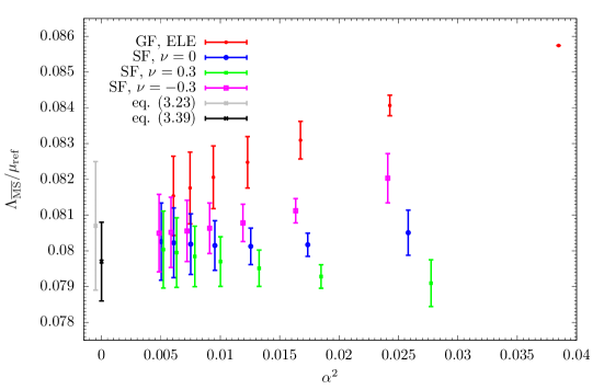
Figure 15: Results for the extraction of $\Lambda_{\overline{\rm MS}}/\mu_{\rm ref}$ based on several schemes, and for different values of the corresponding couplings. The results from the GF coupling refer to its electric scheme and are computed following a step-scaling analysis. At each value of the GF coupling coming from step-scaling, the GF scheme is matched non-perturbatively to three different SF schemes corresponding to $\nu=-0.3,0,0.3$, which are then used to also extract $\Lambda_{\overline{\rm MS}}/\mu_{\rm ref}$. A comparison with our final estimates eqs. (3.23) and (3.39) is given.

In Fig. 15 we present the results based on the SSF of the electric GF scheme. As one can see from the figure, the determination of $\Lambda_{\overline{\rm MS}}/\mu_{\rm ref}$ obtained directly from the GF coupling suffers from large $\mathcal{O}(\alpha^{2})$ corrections. The situation is of course completely analogous to what we already discussed in Sect. 3.4 in terms of the $\beta$-function (cf. Fig. 3). In particular, if we read off the value of $\Lambda_{\overline{\rm MS}}/\mu_{\rm ref}$ for say, $n=6$, the result is:

$${\Lambda_{\overline{\rm MS}}\over\mu_{\rm ref}}=0.0815(11)\,.$$ (C.7)

Although this is compatible with our final estimate, eq. (3.23), it is clear that given the trend of the results for different values of $n$, a reliable determination of both mean value and error, necessarily requires an extrapolation to $\alpha=0$.

Quite different is the situation for the determinations obtained after switching non-perturbatively to the SF couplings. These show indeed much milder $\mathcal{O}(\alpha^{2})$ corrections, particularly so for the case $\nu=0$ (cf. Fig. 4(c)). At values of the coupling $\alpha\sim 0.1$, any discrepancy between different $\nu$-values is negligible within our statistical errors, and we can thus safely quote:

$${\Lambda_{\overline{\rm MS}}\over\mu_{\rm ref}}=0.0802(10)\,,$$ (C.8)

which corresponds to the value obtained for $\nu=0$ at $n=5$. This is in perfect agreement with our final estimate eq. (3.39).

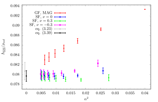
Figure 16: Results for the extraction of $\Lambda_{\overline{\rm MS}}/\mu_{\rm ref}$ based on several schemes, and for different values of the corresponding couplings. The results from the GF coupling refer to its magnetic scheme and are computed following a step-scaling analysis. At each value of the GF coupling coming from step-scaling, the GF scheme is matched non-perturbatively to three different SF schemes corresponding to $\nu=-0.3,0,0.3$, which are then used to also extract $\Lambda_{\overline{\rm MS}}/\mu_{\rm ref}$. A comparison with our final estimates eqs. (3.23) and (3.39) is given.

For completeness we also present in Fig. 16 the corresponding results based on the magnetic GF scheme. It is no surprise that the results for $\Lambda_{\overline{\rm MS}}/\mu_{\rm ref}$ coming from the magnetic coupling show larger $\mathcal{O}(\alpha^{2})$ corrections than what we have seen for the electric scheme (cf. Fig. 3). Considering for instance the results for $n=6$, we have: $\Lambda_{\overline{\rm MS}}/\mu_{\rm ref}=0.0830(10)$, which is clearly biased in both central value and error if compared to eq. (3.23) (note that $\alpha_{\rm GF,\,m}(\mu_{n=6})\sim 0.08$!). On the other hand, once again switching non-perturbatively to the SF schemes solves the issue. Taking for instance the results for $\nu=0$ and $n=5$ we obtain: $\Lambda_{\overline{\rm MS}}/\mu_{\rm ref}=0.0798(9)$, well in agreement with the result of eqs. (3.39) and (C.8). In conclusion, the determination based on the SSF of the GF couplings rather than the $\beta$-function gives perfectly compatible results, reinforcing even further the robustness of our analysis and conclusions.

Appendix D Perturbative improvement of the SF coupling

In this appendix we give some details on the perturbative improvement of the SF coupling in the $\nu=0$ scheme, employed in Sect. 3.5.

In bare lattice perturbation theory, the SF coupling is given by,

$$\bar{g}^{2}_{\rm SF}(L)=g_{0}^{2}+m_{1}(L/a)g_{0}^{4}+m_{2}(L/a)g_{0}^{6}+\mathcal{O}(g_{0}^{8}),$$ (D.1)

where the coefficients of this series can be written as:

$$m_{1} =m_{1}^{a}+c_{t}^{(1)}m_{1}^{b},$$ (D.2)

$$m_{2}-m_{1}^{2} =m_{2}^{a}+c_{t}^{(1)}m_{2}^{b}+[c_{t}^{(1)}]^{2}m_{2}^{c}+c_{t}^{(2)}m_{2}^{d}.$$ (D.3)

Referring to ref. [32] one can easily show that

$$m_{1}^{b}=m_{2}^{d}=-{2a\over L},$$ (D.4)

and

$$m_{2}^{c}={2a\over L}-{4a^{2}\over L^{2}}+\mathcal{O}(a^{5}),$$ (D.5)

which approximation should be good enough in practice. The coefficients $m_{1}^{a}$, $m_{2}^{a}$ and $m_{2}^{b}$ instead can be found in table 1 of ref. [32].

To work out the cutoff effects in the SF coupling to two-loop order we need to know the asymptotic behavior of $m_{1}$ and $m_{2}$ for $L/a\to\infty$. This is given by (see table 2 of ref. [33]):

$$m_{1}^{\infty} =2b_{0}\ln(L/a)+0.36828215(13)+\mathcal{O}(a^{2}),$$ (D.6)

$$m_{2}^{\infty}-[m_{1}^{\infty}]^{2} =2b_{1}\ln(L/a)+0.048091(2)+\mathcal{O}(a^{2}),$$ (D.7)

where $b_{0}$ and $b_{1}$ are the universal one- and two-loop coefficients of the $\beta$-function, eq. (2.5).

Given these results we can define,

$${\bar{g}^{2}_{\rm SF}(L)-\bar{g}^{2}_{{\rm SF},\infty}(L)\over\bar{g}^{2}_{{\rm SF},\infty}(L)}=\delta_{1}(L/a)\,g_{0}^{2}+\delta_{2}(L/a)\,g_{0}^{4}+\mathcal{O}(g_{0}^{6}),$$ (D.8)

where $\bar{g}^{2}_{{\rm SF},\infty}(L)$ as an expansion analogous to (D.1), with the replacement $m_{i}\to m_{i}^{\infty}$, $i=1,2$. It is then easy to show that,

$$\delta_{1}(L/a)=\Delta m_{1},\qquad\delta_{2}(L/a)=\Delta m_{2}-\delta_{1}m_{1}^{\infty},$$ (D.9)

where

$$\Delta m_{i}(L/a)=m_{i}(L/a)-m_{i}^{\infty}(L/a),\quad i=1,2.$$ (D.10)

The corresponding results, taking,

$$c_{t}^{\star}=1-0.08900\,g_{0}^{2}-0.0294\,g_{0}^{4},$$ (D.11)

are given in table 8. A two-loop improved SF coupling can thus be defined as,

$$\bar{g}^{2}_{\rm SF,I}(L)={\bar{g}^{2}_{\rm SF}(L)\over 1+\delta_{1}(L/a)g_{0}^{2}+\delta_{2}(L/a)g_{0}^{4}},$$ (D.12)

or more simply,

$$\bar{g}^{2}_{\rm SF,I}(L)=\bar{g}^{2}_{\rm SF}(L)-\Delta m_{1}(L/a)g_{0}^{4}-\Delta m_{2}(L/a)g_{0}^{6}.$$ (D.13)

The two are of course equivalent up to $\mathcal{O}(g_{0}^{8})$ terms. In Sect. 3.5 we considered the form eq. (D.12). Note that by using eq. (D.1) and the results of Sect. 2.3, we could in principle rexpress the perturbative improvement of the SF coupling in terms the GF couplings, rather than the bare one. Although this might appear more natural when determining the matching between the GF and SF couplings, we prefer not to do so and stick with the bare results. In any case, as already mentioned in the main text, the effect of the perturbative improvement is very small in practice (cf. table 8). Choosing a different option hence does not make any real difference.

$L/a$	$\Delta m_{1}=\delta_{1}$	$\Delta m_{2}$	$\delta_{2}$
4	0.012845313751142	0.015321716769734	0.008110152038992
5	0.007777219114216	0.009579837534989	0.004971807117380
6	0.004974956107720	0.006333958932812	0.003259913472149
7	0.003426899898274	0.004486213192082	0.002295122656827
8	0.002511485605829	0.003360322924560	0.001707808260234
9	0.001927244066032	0.002622904409882	0.001323186298664
10	0.001529846640399	0.002110676347599	0.001056504097430
11	0.001246002180829	0.001738571617701	0.000863443440673
12	0.001035543531126	0.001458806955388	0.000718941170315
13	0.000874854600749	0.001242679157694	0.000607865198940
14	0.000749224845475	0.001071984982022	0.000520595416728
15	0.000649058490722	0.000934670808009	0.000450759687080
16	0.000567859115075	0.000822471509072	0.000393993493151
17	0.000501091899901	0.000729553491342	0.000347222437166
18	0.000445508755510	0.000651697453251	0.000308228470592
19	0.000398731340410	0.000585786821706	0.000275377878968
20	0.000358984476884	0.000529476970044	0.000247445314836
21	0.000324920687670	0.000480975306052	0.000223496862669
22	0.000295501761385	0.000438891494416	0.000202810480112
23	0.000269917024381	0.000402133251700	0.000184820726059
24	0.000247525826056	0.000369832464991	0.000169079640890
25	0.000227816347952	0.000341291913117	0.000155228589411
26	0.000210375634016	0.000315946254512	0.000142977686219
27	0.000194867470794	0.000293333060719	0.000132090551354
28	0.000181015847174	0.000273071038353	0.000122372875705
29	0.000168592437787	0.000254843458832	0.000113663738570
30	0.000157407026808	0.000238385422055	0.000105828951105
31	0.000147300106887	0.000223473964266	0.000098755896729
32	0.000138137105359	0.000209920310316	0.000092349500925

Table 8: Two-loop cutoff effects for the SF coupling with $\nu=0$.

Appendix E Raw the measurement data

E.1 GF coupling

Tables 9 to 16 collect the results of the measurements of the GF couplings for the lattice sizes $L/a=48$, $32$, $24$, $20$, $16$, $12$, $8$, and the corresponding $\beta$ values we have simulated. We list the results for all four coupling definitions and give the total statistics collected in the column labelled by $N_{\rm msm}$. Note that this column also contains in parenthesis the number of measurements for which $|Q|>0.5$, and which thus do not enter the determination of the coupling. Here $Q$ is the topological charge defined through the Zeuthen flow (cf. Sect. 3.1); there are only small differences in the measurements of $Q$ between the Zeuthen and Wilson flow.

E.2 SF coupling

Table 17 contains the results of the measurements of the SF couplings for all the lattice sizes and $\beta$-values we considered, together with the total number of measurements collected, $N_{\rm msm}$; note that all measurements have in this case $Q=0$. We give results for the three values of $\nu=-0.3,0,0.3$, which enter the analysis of Appendix. C. We note that by using any two of these definitions, it is possible to determine the value of the SF coupling and its proper error for any other value of $\nu$ (cf. eq. (2.18) and ref. [7]).

$\beta$	$N_{\rm msm}$	Zeuthen/mag	Wilson/mag	Zeuthen/ele	Wilson/ele
6.7859	2740(2048)	14.353(77)	14.336(76)	14.325(81)	14.307(81)
6.8637	3880(2619)	11.345(63)	11.336(63)	11.363(67)	11.354(67)
6.9595	2040(811)	8.637(39)	8.635(39)	8.539(41)	8.536(41)
7.1146	1560(0)	6.551(17)	6.551(17)	6.438(20)	6.437(20)
7.2000	2100(41)	5.872(13)	5.872(13)	5.765(14)	5.764(14)
7.6000	2300(0)	4.0120(74)	4.0132(74)	3.9334(80)	3.9339(80)
8.0000	3660(0)	3.0886(47)	3.0897(47)	3.0260(51)	3.0267(52)
8.5000	4720(0)	2.4080(29)	2.4090(29)	2.3606(32)	2.3612(32)
9.0000	7220(0)	1.9800(19)	1.9808(19)	1.9448(21)	1.9454(21)
9.5000	9280(0)	1.6860(14)	1.6867(14)	1.6558(16)	1.6563(16)
10.0000	11080(0)	1.4691(11)	1.4697(11)	1.4470(12)	1.4474(12)
10.5000	14700(0)	1.30170(83)	1.30223(83)	1.28435(91)	1.28474(92)
11.0000	18120(0)	1.17159(68)	1.17204(68)	1.15554(74)	1.15587(75)

Table 9: GF coupling data for $L/a=48$.

$\beta$	$N_{\rm msm}$	Zeuthen/mag	Wilson/mag	Zeuthen/ele	Wilson/ele
6.4740	3300(2354)	14.686(70)	14.640(69)	14.690(74)	14.644(73)
6.5619	15350(8273)	10.946(24)	10.930(24)	10.907(25)	10.888(25)
6.6669	1650(246)	8.203(27)	8.201(27)	8.092(32)	8.088(32)
6.7859	1700(9)	6.656(18)	6.657(17)	6.539(19)	6.538(19)
6.8786	1800(10)	5.877(14)	5.879(14)	5.744(16)	5.744(16)
6.9595	1450(0)	5.345(14)	5.348(14)	5.216(14)	5.217(15)
7.1146	2250(0)	4.5866(92)	4.5898(92)	4.4841(99)	4.4855(99)
7.2000	2100(0)	4.2584(87)	4.2617(87)	4.1558(92)	4.1572(92)
7.6000	4450(0)	3.2059(41)	3.2089(42)	3.1362(47)	3.1381(47)
8.0000	7200(0)	2.5918(26)	2.5944(26)	2.5433(28)	2.5450(28)
8.5000	7200(0)	2.0989(20)	2.1011(20)	2.0610(22)	2.0624(22)
9.0000	8700(0)	1.7713(15)	1.7730(15)	1.7375(16)	1.7386(17)
9.5000	12000(0)	1.5319(11)	1.5334(11)	1.5045(12)	1.5056(12)
10.0000	13000(0)	1.35038(91)	1.35164(91)	1.3314(10)	1.3323(10)
10.4258	6000(0)	1.2275(13)	1.2286(13)	1.2115(13)	1.2123(13)
10.5000	17000(0)	1.20874(71)	1.20984(71)	1.19340(78)	1.19421(79)
10.6586	14050(0)	1.17031(76)	1.17134(76)	1.15509(83)	1.15587(84)
11.0000	19350(0)	1.09622(60)	1.09718(60)	1.08289(67)	1.08360(67)

Table 10: GF coupling data for $L/a=32$.

$\beta$	$N_{\rm msm}$	Zeuthen/mag	Wilson/mag	Zeuthen/ele	Wilson/ele
6.2556	5700(4313)	15.307(56)	15.192(54)	15.317(57)	15.198(56)
6.2654	4000(2834)	14.839(59)	14.740(57)	14.851(65)	14.750(63)
6.3451	3200(1792)	11.219(55)	11.193(54)	11.168(60)	11.137(60)
6.3509	3200(1810)	11.044(49)	11.018(49)	10.973(55)	10.945(55)
6.3560	3200(1761)	10.757(53)	10.723(52)	10.687(56)	10.655(54)
6.3642	4000(2040)	10.398(39)	10.380(38)	10.326(43)	10.305(43)
6.4630	3200(635)	8.008(21)	8.007(21)	7.876(23)	7.871(23)
6.5619	6300(316)	6.6813(93)	6.6852(93)	6.555(11)	6.555(11)
6.6559	4000(51)	5.8695(94)	5.8753(94)	5.744(10)	5.746(10)
6.6669	4200(37)	5.7919(92)	5.7974(92)	5.6858(97)	5.6876(98)
6.7859	6400(2)	5.0578(61)	5.0641(61)	4.9486(65)	4.9516(66)
6.8637	6000(0)	4.6776(56)	4.6842(56)	4.5687(60)	4.5718(60)
6.9595	6000(0)	4.2884(51)	4.2950(51)	4.2048(58)	4.2086(58)
7.1146	4000(0)	3.7942(53)	3.8005(53)	3.7197(60)	3.7235(60)
7.2000	10000(0)	3.5705(31)	3.5767(31)	3.4942(34)	3.4980(35)
7.6000	10000(0)	2.8088(24)	2.8141(24)	2.7560(26)	2.7595(26)
8.0000	12900(0)	2.3320(17)	2.3363(17)	2.2895(18)	2.2926(18)
8.5000	14500(0)	1.9284(13)	1.9320(13)	1.8942(14)	1.8967(14)
9.0000	14500(0)	1.6458(11)	1.6488(11)	1.6169(12)	1.6190(12)
9.5000	16000(0)	1.43887(89)	1.44135(90)	1.41746(98)	1.41927(99)
10.0000	19100(0)	1.27695(70)	1.27905(71)	1.26060(78)	1.26212(79)
10.4258	20000(0)	1.16851(64)	1.17034(64)	1.15338(70)	1.15474(71)
10.5000	18800(0)	1.15194(65)	1.15374(65)	1.13672(71)	1.13804(72)
11.0000	21800(0)	1.04784(54)	1.04941(54)	1.03480(59)	1.03598(60)

Table 11: GF coupling data for $L/a=24$.

$\beta$	$N_{\rm msm}$	Zeuthen/mag	Wilson/mag	Zeuthen/ele	Wilson/ele
6.1365	5000(3710)	15.037(59)	14.906(57)	15.016(63)	14.876(62)
6.1700	6000(4110)	13.310(48)	13.201(47)	13.295(51)	13.182(51)
6.2160	5000(2930)	11.181(40)	11.138(38)	11.118(42)	11.066(41)
6.2280	5000(2818)	10.724(39)	10.692(38)	10.668(43)	10.633(42)
6.2556	6000(2658)	9.726(27)	9.707(26)	9.647(30)	9.624(30)
6.4200	6000(286)	6.7554(97)	6.7615(97)	6.620(11)	6.620(11)
6.5197	5000(85)	5.8445(84)	5.8535(84)	5.7207(92)	5.7245(93)
6.5619	6000(50)	5.5487(71)	5.5584(71)	5.4171(76)	5.4210(76)
6.6669	6000(17)	4.9431(61)	4.9532(61)	4.8332(67)	4.8384(68)
6.7859	6000(0)	4.4082(55)	4.4182(55)	4.3157(56)	4.3216(57)
6.8000	6000(11)	4.3553(53)	4.3656(54)	4.2637(55)	4.2698(56)
6.8637	6000(4)	4.1219(48)	4.1319(48)	4.0268(53)	4.0329(53)
6.9595	6000(0)	3.8245(44)	3.8340(44)	3.7398(50)	3.7459(51)
7.1146	6000(0)	3.4254(39)	3.4344(39)	3.3509(40)	3.3566(41)
7.2000	6000(0)	3.2426(36)	3.2513(36)	3.1803(40)	3.1860(41)
7.6000	6000(0)	2.6124(29)	2.6197(29)	2.5547(30)	2.5595(30)
8.0000	8000(0)	2.1908(20)	2.1969(20)	2.1509(21)	2.1552(22)
8.5000	14000(0)	1.8304(12)	1.8353(12)	1.8015(13)	1.8050(13)
9.0000	14000(0)	1.5766(10)	1.5806(10)	1.5521(11)	1.5550(11)
9.5000	14000(0)	1.38439(90)	1.38775(90)	1.36570(98)	1.36819(100)
10.0000	16000(0)	1.23742(76)	1.24027(76)	1.22099(81)	1.22309(83)
10.2830	20000(0)	1.16540(63)	1.16803(63)	1.15006(70)	1.15196(71)
10.5000	20000(0)	1.11778(61)	1.12026(61)	1.10308(65)	1.10490(66)
11.0000	24000(0)	1.01933(51)	1.02149(51)	1.00702(54)	1.00864(55)

Table 12: GF coupling data for $L/a=20$.

$\beta$	$N_{\rm msm}$	Zeuthen/mag	Wilson/mag	Zeuthen/ele	Wilson/ele
5.9900	5000(3782)	15.555(61)	15.285(58)	15.548(62)	15.263(60)
6.0662	5750(3439)	11.331(40)	11.234(38)	11.323(42)	11.221(41)
6.0722	5000(2898)	11.051(42)	10.982(40)	11.023(44)	10.942(43)
6.0740	5000(2850)	10.892(38)	10.832(37)	10.829(41)	10.757(41)
6.1000	5000(2400)	9.894(32)	9.843(31)	9.806(35)	9.749(35)
6.1200	3750(1497)	9.239(31)	9.213(30)	9.124(34)	9.089(33)
6.1700	5750(1272)	7.999(15)	8.005(15)	7.865(17)	7.861(17)
6.2556	5750(319)	6.770(10)	6.783(10)	6.638(11)	6.640(11)
6.3598	5000(61)	5.8085(82)	5.8241(82)	5.6839(88)	5.6908(89)
6.4200	5750(30)	5.3833(70)	5.3999(70)	5.2744(76)	5.2830(77)
6.4740	5000(13)	5.0535(67)	5.0706(67)	4.9430(71)	4.9519(72)
6.4741	10000(28)	5.0594(49)	5.0763(49)	4.9591(51)	4.9683(52)
6.5619	5750(1)	4.6165(56)	4.6335(56)	4.5197(60)	4.5296(62)
6.6669	5000(0)	4.2007(57)	4.2173(57)	4.1056(58)	4.1150(59)
6.7859	6000(0)	3.8249(46)	3.8404(46)	3.7391(48)	3.7488(49)
6.8000	5750(2)	3.7825(44)	3.7980(44)	3.6948(46)	3.7048(47)
6.8637	10000(0)	3.6081(32)	3.6232(32)	3.5222(34)	3.5318(34)
6.8776	7750(0)	3.5765(36)	3.5915(36)	3.5016(38)	3.5112(39)
6.8786	7250(0)	3.5720(37)	3.5871(37)	3.4924(40)	3.5021(41)
6.8787	5000(0)	3.5668(45)	3.5816(46)	3.4991(48)	3.5086(49)
6.9595	5000(0)	3.3744(43)	3.3888(44)	3.3056(48)	3.3147(49)
7.1146	10000(0)	3.0721(26)	3.0854(27)	3.0109(28)	3.0196(29)
7.2000	5750(0)	2.9197(32)	2.9324(32)	2.8614(36)	2.8699(37)
7.6000	6000(0)	2.4044(26)	2.4147(26)	2.3603(27)	2.3676(28)
8.0000	11750(0)	2.0450(15)	2.0537(16)	2.0087(16)	2.0148(16)
8.5000	12000(0)	1.7296(12)	1.7366(12)	1.7003(13)	1.7053(14)
9.0000	12000(0)	1.4976(10)	1.5034(10)	1.4761(11)	1.4802(12)
9.5000	22750(0)	1.32609(68)	1.33083(70)	1.30821(72)	1.31164(74)
10.0000	21000(0)	1.18949(63)	1.19363(63)	1.17455(68)	1.17751(70)
10.1106	20000(0)	1.16469(63)	1.16869(63)	1.14841(67)	1.15129(69)
10.4382	20000(0)	1.09154(59)	1.09517(59)	1.07696(64)	1.07953(66)
10.5000	21000(0)	1.07807(56)	1.08162(57)	1.06517(60)	1.06775(62)
10.6581	3250(0)	1.0466(14)	1.0500(14)	1.0348(15)	1.0372(15)
10.6586	19250(0)	1.04936(58)	1.05279(59)	1.03651(62)	1.03905(64)
10.9270	20000(0)	0.99954(53)	1.00274(53)	0.98835(57)	0.99064(59)
11.0000	23500(0)	0.98731(48)	0.99043(48)	0.97657(52)	0.97890(54)

Table 13: GF coupling data for $L/a=16$.

$\beta$	$N_{\rm msm}$	Zeuthen/mag	Wilson/mag	Zeuthen/ele	Wilson/ele
5.8900	8000(4895)	11.681(37)	11.483(33)	11.679(39)	11.470(36)
5.9000	4800(2823)	11.168(48)	11.003(44)	11.115(49)	10.936(45)
5.9080	1200(644)	10.787(90)	10.639(82)	10.654(91)	10.476(85)
5.9160	7200(3813)	10.291(31)	10.189(29)	10.217(32)	10.105(31)
5.9200	4400(2143)	10.077(38)	9.981(35)	9.983(41)	9.881(38)
5.9900	2000(417)	7.857(26)	7.850(25)	7.730(27)	7.710(26)
6.0000	2000(371)	7.659(26)	7.657(25)	7.528(27)	7.514(27)
6.0662	10000(680)	6.6751(79)	6.6981(78)	6.5575(81)	6.5629(82)
6.1700	10000(118)	5.6802(58)	5.7094(58)	5.5705(61)	5.5841(63)
6.2556	10000(52)	5.1104(49)	5.1414(49)	5.0010(54)	5.0173(56)
6.2643	10000(38)	5.0690(50)	5.1000(50)	4.9572(51)	4.9728(52)
6.2654	10000(37)	5.0489(50)	5.0796(50)	4.9387(51)	4.9552(52)
6.3451	4000(4)	4.6316(71)	4.6621(71)	4.5352(72)	4.5518(74)
6.3509	10000(12)	4.6164(43)	4.6468(44)	4.5206(45)	4.5381(47)
6.3560	4000(2)	4.5905(68)	4.6208(69)	4.4883(73)	4.5050(75)
6.3642	10000(9)	4.5554(44)	4.5853(44)	4.4496(45)	4.4651(46)
6.3894	8800(3)	4.4339(45)	4.4638(45)	4.3433(46)	4.3596(48)
6.4133	10000(1)	4.3543(40)	4.3837(40)	4.2606(42)	4.2771(43)
6.4200	10000(6)	4.3136(40)	4.3434(40)	4.2254(41)	4.2428(43)
6.4630	10000(2)	4.1590(38)	4.1877(38)	4.0659(39)	4.0830(42)
6.5619	10000(0)	3.8287(34)	3.8563(34)	3.7536(35)	3.7707(36)
6.6559	10000(0)	3.5720(31)	3.5983(32)	3.4993(32)	3.5160(34)
6.6566	10000(1)	3.5665(31)	3.5928(31)	3.4926(34)	3.5088(35)
6.6669	10000(1)	3.5441(31)	3.5704(31)	3.4707(32)	3.4864(33)
6.7859	10000(0)	3.2730(30)	3.2973(30)	3.2041(29)	3.2190(31)
6.8000	10000(0)	3.2384(28)	3.2627(28)	3.1699(29)	3.1851(30)
6.8544	8800(0)	3.1382(29)	3.1620(30)	3.0737(30)	3.0884(31)
6.8637	10000(0)	3.1139(27)	3.1371(27)	3.0542(28)	3.0693(29)
6.9595	10000(0)	2.9506(25)	2.9728(25)	2.8908(26)	2.9048(27)
7.1146	10000(0)	2.7085(23)	2.7287(23)	2.6564(24)	2.6696(26)
7.2000	10000(0)	2.6000(22)	2.6195(22)	2.5516(23)	2.5643(24)
7.6000	10000(0)	2.1766(18)	2.1925(18)	2.1431(19)	2.1538(19)
8.0000	10000(0)	1.8809(15)	1.8940(15)	1.8504(15)	1.8591(16)
8.5000	10000(0)	1.6118(13)	1.6225(13)	1.5867(13)	1.5938(14)
9.0000	18250(0)	1.41310(81)	1.42191(82)	1.39153(85)	1.39754(90)
9.5000	18250(0)	1.25790(72)	1.26532(73)	1.24192(74)	1.24710(78)
10.0000	20000(0)	1.13541(61)	1.14181(61)	1.12061(64)	1.12483(67)
10.4250	10000(0)	1.04869(78)	1.05425(79)	1.03752(84)	1.04154(89)
10.4258	18800(0)	1.04795(57)	1.05363(58)	1.03529(63)	1.03909(66)
10.4262	20000(0)	1.04782(56)	1.05344(56)	1.03512(58)	1.03899(61)
10.5000	40000(0)	1.03364(39)	1.03913(39)	1.02089(41)	1.02467(43)
11.0000	20000(0)	0.95006(50)	0.95488(50)	0.93969(53)	0.94299(56)
11.1572	10000(0)	0.92748(69)	0.93213(70)	0.91626(73)	0.91945(76)
12.0000	10000(0)	0.81767(61)	0.82141(62)	0.80886(65)	0.81148(69)

Table 14: GF coupling data for $L/a=12$.

$\beta$	$N_{\rm msm}$	Zeuthen/mag	Wilson/mag	Zeuthen/ele	Wilson/ele
6.0500	6000(89)	5.6477(75)	5.6817(74)	5.5341(81)	5.5437(83)
6.0662	10000(125)	5.5383(59)	5.5741(59)	5.4189(60)	5.4305(62)
6.1000	8000(64)	5.2911(59)	5.3278(59)	5.1751(61)	5.1894(62)
6.1365	20000(72)	5.0562(35)	5.0940(36)	4.9470(36)	4.9627(37)
6.1370	8000(19)	5.0551(56)	5.084(11)	4.9433(57)	4.949(11)
6.1500	8000(21)	4.9756(54)	5.000(16)	4.8670(54)	4.870(15)
6.1700	10000(25)	4.8639(46)	4.9023(46)	4.7576(48)	4.7735(50)
6.2000	8000(16)	4.7104(52)	4.679(67)	4.6016(51)	4.552(66)
6.2160	20000(32)	4.6283(31)	4.6669(31)	4.5320(31)	4.5500(33)
6.2280	20000(25)	4.5814(31)	4.6201(32)	4.4797(32)	4.4981(33)
6.2556	10000(8)	4.4561(42)	4.4939(43)	4.3571(42)	4.3759(44)
6.4200	10000(0)	3.8494(34)	3.8854(35)	3.7677(35)	3.7870(37)
6.4589	40000(3)	3.7357(16)	3.7711(17)	3.6584(17)	3.6779(18)
6.5081	20000(1)	3.5991(22)	3.6337(23)	3.5227(23)	3.5416(24)
6.5197	20000(0)	3.5698(22)	3.6040(23)	3.4986(23)	3.5173(24)
6.5209	20000(1)	3.5686(22)	3.6031(23)	3.4932(23)	3.5122(24)
6.5573	40000(0)	3.4789(15)	3.5127(15)	3.4056(16)	3.4246(16)
6.5619	10000(0)	3.4562(31)	3.4900(31)	3.3830(31)	3.4010(32)
6.5871	10000(0)	3.4039(30)	3.4369(31)	3.3359(31)	3.3549(33)
6.6669	10000(0)	3.2287(28)	3.2604(28)	3.1602(28)	3.1784(30)
6.7543	26000(0)	3.0621(16)	3.0922(16)	3.0015(16)	3.0189(17)
6.7859	10000(0)	3.0048(26)	3.0344(27)	2.9416(26)	2.9581(27)
6.8000	10000(0)	2.9811(25)	3.0107(26)	2.9205(25)	2.9378(27)
6.8036	26000(0)	2.9740(16)	3.0033(16)	2.9153(16)	2.9320(17)
6.8528	26000(0)	2.8940(15)	2.9226(16)	2.8355(15)	2.8521(16)
6.8637	20000(0)	2.8723(17)	2.9007(17)	2.8172(17)	2.8341(18)
6.9595	10000(0)	2.7283(23)	2.7551(23)	2.6776(23)	2.6934(24)
7.1146	10000(0)	2.5282(21)	2.5529(21)	2.4804(21)	2.4954(22)
7.2000	10000(0)	2.4279(20)	2.4516(20)	2.3842(20)	2.3987(21)
7.6000	10000(0)	2.0640(16)	2.0835(17)	2.0277(17)	2.0393(18)
8.0000	15000(0)	1.7960(11)	1.8122(12)	1.7661(12)	1.7761(12)
8.5000	15000(0)	1.54889(97)	1.56216(100)	1.52559(100)	1.5339(11)
9.0000	20000(0)	1.36404(72)	1.37499(74)	1.34555(75)	1.35247(81)
9.5000	20000(0)	1.22019(67)	1.22942(69)	1.20446(69)	1.21022(74)
10.0000	20000(0)	1.10469(58)	1.11268(60)	1.09035(60)	1.09538(64)
10.2155	20000(0)	1.06058(55)	1.06805(56)	1.04732(57)	1.05210(62)
10.2682	20000(0)	1.05109(57)	1.05847(58)	1.03900(56)	1.04377(61)
10.2830	20000(0)	1.04805(54)	1.05547(56)	1.03521(57)	1.04001(61)
10.2862	40000(0)	1.04684(38)	1.05418(39)	1.03428(41)	1.03895(44)
10.3209	10000(0)	1.04153(76)	1.04881(78)	1.02809(80)	1.03265(85)
10.5000	50000(0)	1.00839(33)	1.01530(34)	0.99639(34)	1.00078(37)
11.0000	30000(0)	0.92827(39)	0.93434(40)	0.91824(41)	0.92211(44)

Table 15: GF coupling data for $L/a=10$.

$\beta$	$N_{\rm msm}$	Zeuthen/mag	Wilson/mag	Zeuthen/ele	Wilson/ele
5.9600	10000(52)	5.2580(55)	5.2711(54)	5.1504(54)	5.1243(56)
5.9900	10000(40)	5.0579(52)	5.0761(52)	4.9452(52)	4.9253(54)
6.0662	15000(21)	4.6269(36)	4.6546(37)	4.5251(35)	4.5168(38)
6.1287	10000(3)	4.3399(41)	4.3707(42)	4.2508(40)	4.2493(43)
6.1700	15000(3)	4.1717(31)	4.2039(32)	4.0853(31)	4.0870(33)
6.2556	15000(4)	3.8730(29)	3.9061(30)	3.7952(29)	3.7998(31)
6.3597	10000(0)	3.5727(31)	3.6066(32)	3.5005(31)	3.5078(33)
6.3604	10000(0)	3.5669(31)	3.6004(32)	3.4915(31)	3.4996(33)
6.4147	10000(0)	3.4283(30)	3.4612(32)	3.3624(29)	3.3697(32)
6.4198	10000(0)	3.4135(29)	3.4465(30)	3.3457(29)	3.3535(31)
6.4200	15000(0)	3.4194(24)	3.4526(25)	3.3492(23)	3.3568(26)
6.5619	15000(0)	3.1157(22)	3.1476(23)	3.0525(21)	3.0619(23)
6.7859	15000(0)	2.7432(19)	2.7731(20)	2.6887(18)	2.6985(20)
6.8000	15000(0)	2.7208(18)	2.7502(19)	2.6715(18)	2.6816(20)
6.8637	15000(0)	2.6403(17)	2.6689(18)	2.5885(17)	2.5989(19)
7.0425	10000(0)	2.4210(19)	2.4476(20)	2.3789(19)	2.3889(21)
7.1146	15000(0)	2.3450(15)	2.3707(16)	2.3044(15)	2.3145(17)
7.2000	15000(0)	2.2605(15)	2.2851(15)	2.2221(14)	2.2320(16)
7.6000	15000(0)	1.9404(12)	1.9609(13)	1.9103(12)	1.9196(13)
8.0000	15000(0)	1.7038(10)	1.7215(11)	1.6769(11)	1.6848(12)
8.5000	15000(0)	1.47990(90)	1.49457(96)	1.45938(89)	1.4659(10)
9.0000	35000(0)	1.31185(52)	1.32419(55)	1.29494(52)	1.30076(58)
9.5000	35000(0)	1.17746(46)	1.18801(48)	1.16411(45)	1.16930(51)
9.8663	20000(0)	1.09624(55)	1.10574(58)	1.08359(58)	1.08807(65)
10.0000	35000(0)	1.06989(41)	1.07906(44)	1.05719(42)	1.06163(47)
10.1102	1000(0)	1.0440(25)	1.009(44)	1.0347(25)	0.994(44)
10.1127	50000(0)	1.04689(34)	1.05573(36)	1.03593(34)	1.04027(38)
10.1184	40000(0)	1.04653(38)	1.05531(40)	1.03508(38)	1.03936(42)
10.5000	35000(0)	0.97920(38)	0.98716(40)	0.96872(38)	0.97257(42)
11.0000	35000(0)	0.90360(35)	0.91066(37)	0.89447(35)	0.89798(39)
12.0000	10000(0)	0.78447(54)	0.79008(57)	0.77644(56)	0.77901(64)
12.6814	20000(0)	0.71847(36)	0.72333(38)	0.71220(36)	0.71457(41)
13.0000	10000(0)	0.69193(49)	0.69649(51)	0.68663(51)	0.68868(57)

Table 16: GF coupling data for $L/a=8$.

$L/a$	$\beta$	$N_{\rm msm}$	$\bar{g}^{2}_{{\rm SF},\nu=0}$	$\bar{g}^{2}_{{\rm SF},\nu=0.3}$	$\bar{g}^{2}_{{\rm SF},\nu=-0.3}$
$6$	$7.6000$	$450000$	$1.7804(12)$	$1.8434(15)$	$1.7216(13)$
$6$	$8.0000$	$450000$	$1.57426(96)$	$1.6256(12)$	$1.5260(10)$
$6$	$8.5000$	$450000$	$1.37634(76)$	$1.41721(94)$	$1.33776(83)$
$6$	$9.0000$	$450000$	$1.22595(62)$	$1.25857(77)$	$1.19498(69)$
$6$	$9.5000$	$450000$	$1.10542(52)$	$1.13184(65)$	$1.08020(58)$
$6$	$10.0000$	$450000$	$1.00866(45)$	$1.03106(55)$	$0.98722(50)$
$6$	$10.4250$	$450000$	$0.93785(40)$	$0.95775(49)$	$0.91876(45)$
$6$	$10.4262$	$450000$	$0.93791(40)$	$0.95684(49)$	$0.91971(44)$
$6$	$10.5000$	$450000$	$0.92709(39)$	$0.94634(48)$	$0.90860(44)$
$6$	$11.0000$	$450000$	$0.85873(34)$	$0.87512(42)$	$0.84293(38)$
$8$	$7.6000$	$500000$	$1.9309(17)$	$2.0017(20)$	$1.8649(18)$
$8$	$8.0000$	$500000$	$1.6887(13)$	$1.7451(16)$	$1.6358(14)$
$8$	$8.5000$	$500000$	$1.4604(10)$	$1.5050(12)$	$1.4185(11)$
$8$	$9.0000$	$600000$	$1.29090(76)$	$1.32602(92)$	$1.25759(83)$
$8$	$9.5000$	$600000$	$1.15884(63)$	$1.18762(77)$	$1.13143(70)$
$8$	$10.0000$	$600000$	$1.05174(53)$	$1.07564(65)$	$1.02887(59)$
$8$	$10.1106$	$600000$	$1.03063(52)$	$1.05355(63)$	$1.00869(58)$
$8$	$10.4382$	$600000$	$0.97373(47)$	$0.99467(58)$	$0.95366(52)$
$8$	$10.5000$	$600000$	$0.96384(46)$	$0.98406(56)$	$0.94444(52)$
$8$	$10.6581$	$600000$	$0.93870(44)$	$0.95733(54)$	$0.92078(49)$
$8$	$10.9270$	$600000$	$0.89861(42)$	$0.91589(50)$	$0.88197(46)$
$8$	$11.0000$	$600000$	$0.88910(41)$	$0.90618(49)$	$0.87265(45)$
$10$	$8.0000$	$900000$	$1.7927(13)$	$1.8556(16)$	$1.7339(14)$
$10$	$8.5000$	$900000$	$1.53723(100)$	$1.5855(12)$	$1.4918(11)$
$10$	$9.0000$	$900000$	$1.34989(80)$	$1.38745(96)$	$1.31431(87)$
$10$	$9.5000$	$900000$	$1.20415(66)$	$1.23490(80)$	$1.17490(72)$
$10$	$10.0000$	$900000$	$1.08927(56)$	$1.11425(67)$	$1.06538(61)$
$10$	$10.5000$	$900000$	$0.99465(48)$	$1.01561(58)$	$0.97454(53)$
$10$	$11.0000$	$900000$	$0.91528(42)$	$0.93277(51)$	$0.89844(47)$
$12$	$8.0000$	$1200000$	$1.8880(14)$	$1.9544(17)$	$1.8259(15)$
$12$	$8.5000$	$1200000$	$1.6070(11)$	$1.6568(13)$	$1.5601(12)$
$12$	$9.0000$	$1200000$	$1.40143(85)$	$1.4413(10)$	$1.36372(92)$
$12$	$9.5000$	$1200000$	$1.24490(69)$	$1.27658(83)$	$1.21474(75)$
$12$	$10.0000$	$1200000$	$1.12205(59)$	$1.14851(70)$	$1.09679(64)$
$12$	$10.4258$	$1200000$	$1.03544(51)$	$1.05795(61)$	$1.01386(56)$
$12$	$10.5000$	$1200000$	$1.02105(50)$	$1.04306(60)$	$0.99996(55)$
$12$	$11.0000$	$1200000$	$0.93837(43)$	$0.95710(52)$	$0.92036(48)$
$16$	$8.5000$	$1600000$	$1.7293(13)$	$1.7877(16)$	$1.6745(14)$
$16$	$9.0000$	$1600000$	$1.4940(10)$	$1.5382(12)$	$1.4524(11)$
$16$	$9.5000$	$1600000$	$1.31496(81)$	$1.34929(96)$	$1.28233(87)$
$16$	$10.0000$	$1600000$	$1.17831(68)$	$1.20691(80)$	$1.15104(73)$
$16$	$10.4258$	$1800000$	$1.08260(55)$	$1.10666(65)$	$1.05956(60)$
$16$	$10.5000$	$1800000$	$1.06889(54)$	$1.09233(64)$	$1.04644(59)$
$16$	$10.6581$	$1800000$	$1.03762(52)$	$1.06036(61)$	$1.01584(56)$
$16$	$11.0000$	$2000000$	$0.97567(44)$	$0.99547(52)$	$0.95664(48)$

Table 17: SF coupling data.

References

- [1] D. J. Gross and F. Wilczek, “Ultraviolet behavior of non-abelian gauge theories,” Phys. Rev. Lett. 30 (June, 1973) 1343–1346.
- [2] H. D. Politzer, “Reliable perturbative results for strong interactions?,” Phys. Rev. Lett. 30 (June, 1973) 1346–1349.
- [3] K. G. Wilson, “Quantum chromodynamics on a lattice,”. Presented at Cargese Summer Inst., Cargese, France, Jul 12- 31, 1976.
- [4] M. Creutz, “Monte Carlo Study of Quantized SU(2) Gauge Theory,” Phys.Rev. D21 (1980) 2308–2315.
- [5] M. Lüscher, P. Weisz, and U. Wolff, “A Numerical method to compute the running coupling in asymptotically free theories,” Nucl.Phys. B359 (1991) 221–243.
- [6] M. Lüscher, R. Narayanan, P. Weisz, and U. Wolff, “The Schrödinger Functional: a renormalizable probe for non-abelian gauge theories,” Nucl.Phys. B384 (1992) 168–228, arXiv:hep-lat/9207009 [hep-lat].
- [7] ALPHA Collaboration, M. Dalla Brida, P. Fritzsch, T. Korzec, A. Ramos, S. Sint, and R. Sommer, “A non-perturbative exploration of the high energy regime in QCD,” Eur. Phys. J. C78 no. 5, (2018) 372, arXiv:1803.10230 [hep-lat].
- [8] ALPHA Collaboration, M. Dalla Brida, P. Fritzsch, T. Korzec, A. Ramos, S. Sint, and R. Sommer, “Determination of the QCD -parameter and the accuracy of perturbation theory at high energies,” Phys. Rev. Lett. 117 no. 18, (2016) 182001, arXiv:1604.06193 [hep-ph].
- [9] M. Lüscher, R. Sommer, P. Weisz, and U. Wolff, “A precise determination of the running coupling in the SU(3) Yang-Mills theory,” Nucl.Phys. B413 (1994) 481–502, arXiv:hep-lat/9309005 [hep-lat].
- [10] R. Narayanan and H. Neuberger, “Infinite N phase transitions in continuum Wilson loop operators,” JHEP 0603 (2006) 064, arXiv:hep-th/0601210 [hep-th].
- [11] M. Lüscher, “Properties and uses of the Wilson flow in lattice QCD,” JHEP 1008 (2010) 071, arXiv:1006.4518 [hep-lat].
- [12] Z. Fodor, K. Holland, J. Kuti, D. Nogradi, and C. H. Wong, “The Yang-Mills gradient flow in finite volume,” JHEP 1211 (2012) 007, arXiv:1208.1051 [hep-lat].
- [13] P. Fritzsch and A. Ramos, “The gradient flow coupling in the Schrödinger Functional,” JHEP 1310 (2013) 008, arXiv:1301.4388 [hep-lat].
- [14] A. Ramos, “The gradient flow running coupling with twisted boundary conditions,” JHEP 1411 (2014) 101, arXiv:1409.1445 [hep-lat].
- [15] A. Ramos, “The Yang-Mills gradient flow and renormalization,” PoS LATTICE2014 (2015) 017, arXiv:1506.00118 [hep-lat].
- [16] A. Ramos and S. Sint, “Symanzik improvement of the gradient flow in lattice gauge theories,” Eur. Phys. J. C76 no. 1, (2016) 15, arXiv:1508.05552 [hep-lat].
- [17] R. V. Harlander and T. Neumann, “The perturbative QCD gradient flow to three loops,” JHEP 06 (2016) 161, arXiv:1606.03756 [hep-ph].
- [18] Dalla Brida, Mattia and Lüscher, Martin, “SMD-based numerical stochastic perturbation theory,” Eur. Phys. J. C77 no. 5, (2017) 308, arXiv:1703.04396 [hep-lat].
- [19] ALPHA Collaboration, M. Dalla Brida, P. Fritzsch, T. Korzec, A. Ramos, S. Sint, and R. Sommer, “Slow running of the Gradient Flow coupling from 200 MeV to 4 GeV in QCD,” Phys. Rev. D95 no. 1, (2017) 014507, arXiv:1607.06423 [hep-lat].
- [20] ALPHA Collaboration, M. Bruno, M. Dalla Brida, P. Fritzsch, T. Korzec, A. Ramos, S. Schaefer, H. Simma, S. Sint, and R. Sommer, “QCD Coupling from a Nonperturbative Determination of the Three-Flavor Parameter,” Phys. Rev. Lett. 119 no. 10, (2017) 102001, arXiv:1706.03821 [hep-lat].
- [21] ALPHA Collaboration, T. Korzec, “Determination of the Strong Coupling Constant by the ALPHA Collaboration,” EPJ Web Conf. 175 (2018) 01018, arXiv:1711.01084 [hep-lat].
- [22] ALPHA Collaboration, M. Dalla Brida, “Precision Determination of from Lattice QCD,” Universe 4 no. 12, (2018) 148, arXiv:1812.06692 [hep-ph].
- [23] T. van Ritbergen, J. A. M. Vermaseren, and S. A. Larin, “The Four loop beta function in quantum chromodynamics,” Phys. Lett. B400 (1997) 379–384, arXiv:hep-ph/9701390 [hep-ph].
- [24] M. Czakon, “The Four-loop QCD beta-function and anomalous dimensions,” Nucl. Phys. B710 (2005) 485–498, arXiv:hep-ph/0411261 [hep-ph].
- [25] P. A. Baikov, K. G. Chetyrkin, and J. H. Kḧn, “Five-Loop Running of the QCD coupling constant,” Phys. Rev. Lett. 118 no. 8, (2017) 082002, arXiv:1606.08659 [hep-ph].
- [26] T. Luthe, A. Maier, P. Marquard, and Y. Schröder, “Towards the five-loop Beta function for a general gauge group,” JHEP 07 (2016) 127, arXiv:1606.08662 [hep-ph].
- [27] F. Herzog, B. Ruijl, T. Ueda, J. A. M. Vermaseren, and A. Vogt, “The five-loop beta function of Yang-Mills theory with fermions,” JHEP 02 (2017) 090, arXiv:1701.01404 [hep-ph].
- [28] R. Sommer, “A New way to set the energy scale in lattice gauge theories and its applications to the static force and alpha-s in SU(2) Yang-Mills theory,” Nucl. Phys. B411 (1994) 839–854, arXiv:hep-lat/9310022 [hep-lat].
- [29] A. Gonzalez-Arroyo, J. Jurkiewicz, and C. Korthals-Altes, “Ground state metamorphosis for Yang-Mills fields on a finite periodic lattice,” Freiburg ASI 1981:0339 (1981) .
- [30] S. Sint and R. Sommer, “The Running coupling from the QCD Schrodinger functional: A One loop analysis,” Nucl. Phys. B465 (1996) 71–98, arXiv:hep-lat/9508012 [hep-lat].
- [31] S. Sint and P. Vilaseca, “Lattice artefacts in the Schródinger Functional coupling for strongly interacting theories,” PoS LATTICE2012 (2012) 031, arXiv:1211.0411 [hep-lat].
- [32] Alpha Collaboration, A. Bode, U. Wolff, and P. Weisz, “Two loop computation of the Schrodinger functional in pure SU(3) lattice gauge theory,” Nucl. Phys. B540 (1999) 491–499, arXiv:hep-lat/9809175 [hep-lat].
- [33] ALPHA Collaboration, A. Bode, P. Weisz, and U. Wolff, “Two loop computation of the Schrodinger functional in lattice QCD,” Nucl. Phys. B576 (2000) 517–539, arXiv:hep-lat/9911018 [hep-lat]. [Erratum: Nucl. Phys.B600,453(2001)].
- [34] ALPHA Collaboration, M. Della Morte et al., “Computation of the strong coupling in QCD with two dynamical flavors,” Nucl.Phys. B713 (2005) 378–406, arXiv:hep-lat/0411025 [hep-lat].
- [35] O. V. Tarasov, A. A. Vladimirov, and A. Yu. Zharkov, “The Gell-Mann-Low Function of QCD in the Three Loop Approximation,” Phys. Lett. 93B (1980) 429–432.
- [36] S. A. Larin and J. A. M. Vermaseren, “The Three loop QCD Beta function and anomalous dimensions,” Phys. Lett. B303 (1993) 334–336, arXiv:hep-ph/9302208 [hep-ph].
- [37] M. Lüscher and P. Weisz, “Perturbative analysis of the gradient flow in non-abelian gauge theories,” JHEP 1102 (2011) 051, arXiv:1101.0963 [hep-th].
- [38] E. I. Bribian and M. Garcia Perez, “The twisted gradient flow coupling at one loop,” arXiv:1903.08029 [hep-lat].
- [39] M. Dalla Brida and D. Hesse, “Numerical Stochastic Perturbation Theory and the Gradient Flow,” PoS Lattice2013 (2014) 326, arXiv:1311.3936 [hep-lat].
- [40] M. Dalla Brida and M. Lüscher, “The gradient flow coupling from numerical stochastic perturbation theory,” PoS LATTICE2016 (2016) 332, arXiv:1612.04955 [hep-lat].
- [41] M. Dalla Brida, M. Garofalo, and A. D. Kennedy, “Investigation of New Methods for Numerical Stochastic Perturbation Theory in Theory,” Phys. Rev. D96 no. 5, (2017) 054502, arXiv:1703.04406 [hep-lat].
- [42] M. Lüscher, R. Sommer, U. Wolff, and P. Weisz, “Computation of the running coupling in the SU(2) Yang-Mills theory,” Nucl.Phys. B389 (1993) 247–264, arXiv:hep-lat/9207010 [hep-lat].
- [43] M. Lüscher, “Step scaling and the Yang-Mills gradient flow,” JHEP 1406 (2014) 105, arXiv:1404.5930 [hep-lat].
- [44] M. Lüscher and P. Weisz, “On-Shell Improved Lattice Gauge Theories,” Commun.Math.Phys. 97 (1985) 59.
- [45] L. Del Debbio, G. M. Manca, and E. Vicari, “Critical slowing down of topological modes,” Phys.Lett. B594 (2004) 315–323, arXiv:hep-lat/0403001 [hep-lat].
- [46] P. Fritzsch, A. Ramos, and F. Stollenwerk, “Critical slowing down and the gradient flow coupling in the Schrödinger functional,” PoS Lattice2013 (2013) 461, arXiv:1311.7304 [hep-lat].
- [47] A. Rubeo and S. Sint, “Perturbative O() effects in gradient flow couplings with SF and SF-open boundary conditions,” PoS LATTICE2016 (2016) 388, arXiv:1612.07047 [hep-lat].
- [48] K. Fabricius and O. Haan, “Heat Bath Method for the Twisted Eguchi-Kawai Model,” Phys.Lett. B143 (1984) 459.
- [49] A. Kennedy and B. Pendleton, “Improved Heat Bath Method for Monte Carlo Calculations in Lattice Gauge Theories,” Phys.Lett. B156 (1985) 393–399.
- [50] M. Creutz, “Overrelaxation and Monte Carlo Simulation,” Phys.Rev. D36 (1987) 515.
- [51] U. Wolff, “Dynamics of hybrid overrelaxation in the Gaussian model,” Phys.Lett. B288 (1992) 166–170.
- [52] N. Madras and A. D. Sokal, “The pivot algorithm: A highly efficient monte carlo method for the self-avoiding walk,” Journal of Statistical Physics 50 no. 1, (Jan, 1988) 109–186. https://doi.org/10.1007/BF01022990.
- [53] ALPHA Collaboration, U. Wolff, “Monte Carlo errors with less errors,” Comput.Phys.Commun. 156 (2004) 143–153, arXiv:hep-lat/0306017 [hep-lat].
- [54] ALPHA Collaboration, S. Schaefer, R. Sommer, and F. Virotta, “Critical slowing down and error analysis in lattice QCD simulations,” Nucl. Phys. B845 (2011) 93–119, arXiv:1009.5228 [hep-lat].
- [55] A. Ramos, “Automatic differentiation for error analysis of Monte Carlo data,” Comput. Phys. Commun. 238 (2019) 19–35, arXiv:1809.01289 [hep-lat].
- [56] R. Sommer, F. Tekin, and U. Wolff, “Running of the SF-coupling with four massless flavours,” PoS LATTICE2010 (2010) 241, arXiv:1011.2332 [hep-lat].
- [57] Giusti, Leonardo and Lüscher, Martin, “Topological susceptibility at from master-field simulations of the SU(3) gauge theory,” arXiv:1812.02062 [hep-lat].
- [58] ALPHA Collaboration, F. Knechtli, T. Korzec, B. Leder, and G. Moir, “Power corrections from decoupling of the charm quark,” Phys. Lett. B774 (2017) 649–655, arXiv:1706.04982 [hep-lat].
- [59] ALPHA Collaboration, M. Guagnelli, R. Sommer, and H. Wittig, “Precision computation of a low-energy reference scale in quenched lattice QCD,” Nucl. Phys. B535 (1998) 389–402, arXiv:hep-lat/9806005 [hep-lat].
- [60] S. Necco and R. Sommer, “The N(f) = 0 heavy quark potential from short to intermediate distances,” Nucl. Phys. B622 (2002) 328–346, arXiv:hep-lat/0108008 [hep-lat].
- [61] Flavour Lattice Averaging Group Collaboration, S. Aoki et al., “FLAG Review 2019,” arXiv:1902.08191 [hep-lat].
- [62] ALPHA Collaboration, S. Capitani, M. Lüscher, R. Sommer, and H. Wittig, “Non-perturbative quark mass renormalization in quenched lattice QCD,” Nucl.Phys. B544 (1999) 669–698, arXiv:hep-lat/9810063 [hep-lat].
- [63] M. Gockeler, R. Horsley, A. C. Irving, D. Pleiter, P. E. L. Rakow, G. Schierholz, and H. Stuben, “A Determination of the Lambda parameter from full lattice QCD,” Phys. Rev. D73 (2006) 014513, arXiv:hep-ph/0502212 [hep-ph].
- [64] N. Brambilla, X. Garcia i Tormo, J. Soto, and A. Vairo, “Precision determination of from the QCD static energy,” Phys. Rev. Lett. 105 (2010) 212001, arXiv:1006.2066 [hep-ph]. [Erratum: Phys. Rev. Lett.108,269903(2012)].
- [65] M. Asakawa, T. Hatsuda, T. Iritani, E. Itou, M. Kitazawa, and H. Suzuki, “Determination of Reference Scales for Wilson Gauge Action from Yang–Mills Gradient Flow,” arXiv:1503.06516 [hep-lat].
- [66] M. Kitazawa, T. Iritani, M. Asakawa, T. Hatsuda, and H. Suzuki, “Equation of State for SU(3) Gauge Theory via the Energy-Momentum Tensor under Gradient Flow,” Phys. Rev. D94 no. 11, (2016) 114512, arXiv:1610.07810 [hep-lat].
- [67] K.-I. Ishikawa, I. Kanamori, Y. Murakami, A. Nakamura, M. Okawa, and R. Ueno, “Non-perturbative determination of the -parameter in the pure SU(3) gauge theory from the twisted gradient flow coupling,” JHEP 12 (2017) 067, arXiv:1702.06289 [hep-lat].
- [68] A. Athenodorou, J. Finkenrath, F. Knechtli, T. Korzec, B. Leder, M. K. Marinkovic, and R. Sommer, “How perturbative are heavy sea quarks?,” arXiv:1809.03383 [hep-lat].
- [69] Z. Fodor, K. Holland, J. Kuti, S. Mondal, D. Nogradi, et al., “The lattice gradient flow at tree-level and its improvement,” JHEP 1409 (2014) 018, arXiv:1406.0827 [hep-lat].