Fluid Structure Interaction modelling using Lattice Boltzmann and Volume Penalization method

Abstract

This paper proposes an approach combining the Volume Penalization (VP) and the the Lattice Boltzmann method (LBM) to compute fluid structure interaction involving rigid bodies. The method consists in adding a force term in the LBM formulation, and thus considers the rigid body similar to particular porous media. Using a characteristic function for the solid domain avoids the expensive tracking of the fluid-solid interface employed commonly in LBM to treat FSI problems. The method is applied to three FSI problems and solved using a Graphics Processor Units (GPU) device. The applications focus on the capacity of the method to compute the drag and lift coefficients for various cases : the imposed displacement of a cylinder, the particle sedimentation at a very low Reynolds number and the VIV of a cylinder in a transverse fluid flow. For all cases the VP-LBM approach yields results which are in a good agreement with those of literature.

Keyword

Lattice Boltzmann Method, Fluid Structure Interaction, Volume Penalization, Vortex Induced Vibration (VIV)

1 Introduction

In the following section, the mathematical background is presented. This part deals with the Lattice Boltzmann Method and more particularly the Multiple Relaxation Time (MRT) approach, the Volume Penalization and how these two methods are combined. The last section presents computational applications computed on a GPU device. For the first tested case, the imposed displacement of a cylinder in a transverse fluid flow at a Reynolds of $100$, is not a real case of FSI. This application enables to validate the capacity of the method to compute drag and lift forces. The second example deals with particle sedimentation under gravity, the particle is free to move under fluid and gravity constraints and complex trajectories can be obtained. The last application focuses on the behavior of the VP-LBM method for FSI problems when a parameter is varied. The stiffness parameter of a free oscillating cylinder in a transverse fluid flow is changed, and the capacity of the VP-LBM to reproduce results from the literature is evaluated.

2 Governing equations

In this section, the numerical models are exposed. The following notations are used : $\rho$ and $\mathbf{u}$ are the macroscopic density and velocity, and bold characters denote vectors.

2.1 Volume penalization

Let us consider a fluid domain $\Omega_{f}$, a solid domain $\Omega_{s}$, $\Gamma$ the fluid-solid interface, and let us note $\Omega=\Omega_{f}\cup\Omega_{s}\cup\Gamma$. The Volume Penalization (VP) method consists in extending the Navier-Stokes equations on the whole domain $\Omega$, and considering the solid domain as a porous medium with a very small permeability. The method was introduced by Angot et al. [11] and already applied to macroscopic equations for moving bodies [14]. The small permeability of the solid domain is modelled using a penalization coefficient, hence the desired boundary conditions at the fluid-solid interface are naturally imposed. With this method, the incompressible Navier-Stokes equations are written as follows :

$$\begin{array}[]{ll}\displaystyle\nabla\cdot\mathbf{u}=0\\ \displaystyle\frac{\partial\mathbf{u}}{\partial t}+\mathbf{u}\cdot\nabla\mathbf{u}=\displaystyle-\frac{1}{\rho}\nabla p+\nu\nabla^{2}\mathbf{u}-\dfrac{\chi_{\Omega_{s}}}{\eta}\left(\mathbf{u}-\mathbf{u_{s}}\right)\\ \end{array}$$ (1)

where

$$\chi_{\Omega_{s}}\left(\boldsymbol{x},t\right)=\left\{\begin{array}[]{ll}1\;\;\textrm{if}\;\;\boldsymbol{x}\in\Omega_{s}\left(t\right)\\ 0\;\;\textrm{otherwise}\end{array}\right.;\hskip 28.45274pt\eta\ll 1\;\;\textrm{penalization factor}$$ (2)

$\mathbf{u}$ denotes the velocity field, $p$ is the pressure field, $\rho$ and $\nu$ are the density and the viscosity of the fluid. $\mathbf{F}=\dfrac{\chi_{\Omega_{s}}}{\eta}\left(\mathbf{u}-\mathbf{u_{s}}\right)$ is the penalization term, and $\mathbf{u_{s}}$ is the velocity field in the solid domain.

2.2 Lattice Boltzmann method

Based on the Boltzmann equation (equation (3)) proposed in the context of the Kinetic Gaz Theory by L. Boltzmann in 1870, the Lattice Boltzmann Method has been successfully used to model fluid flow since the 90’s

$$\dfrac{\partial f}{\partial t}+\mathbf{c}\cdot\nabla_{x}f=\Omega\left(f\right)$$ (3)

This equation models the transport of $f\left(\boldsymbol{x},t,\mathbf{c}\right)$, a probability density function to find a particle at location $\boldsymbol{x}$ and time $t$ with the velocity $\mathbf{c}$, $\Omega\left(f\right)$ being a collision operator. The link between the Boltzmann equation and the Navier-Stokes equations is well-known since the Chapmann-Enskog expansion proposed in 1915.
The Lattice Boltzmann method considers the discretization of equation (3) according to space and velocity and leads to the following discretized equations :

$$f_{\alpha}\left(\boldsymbol{x}+\mathbf{c_{\alpha}}\triangle t,t+\triangle t\right)-f_{\alpha}\left(\boldsymbol{x},t\right)=\Omega_{\alpha}\left(f\right)+\triangle tF_{\alpha}$$ (4)

where $\displaystyle f_{\alpha}\left(\boldsymbol{x},t\right)=\displaystyle f\left(\boldsymbol{x},\mathbf{c_{\alpha}},t\right)$, $\displaystyle F_{\alpha}$ is a forcing term related to the discrete velocity $\mathbf{c_{\alpha}}$. The first model proposed by Bhatnagar et al. [15] is the BGK model which is based on a linear collision operator with a single relaxation time :

$$\Omega_{\alpha}\left(f\right)=-\dfrac{1}{\tau}\left(f_{\alpha}\left(\boldsymbol{x},t\right)-f^{\textrm{eq}}_{\alpha}\left(\boldsymbol{x},t\right)\right)$$ (5)

where $f^{\textrm{eq}}$ is the equilibrium function and $\tau$ is the non dimensional relaxation time which is linked to the fluid viscosity as follows (6).

$$\nu=c^{2}_{s}\triangle t\left(\tau-\dfrac{1}{2}\right)$$ (6)

We propose in this paper to use the Multiple Relaxation Time (MRT) model, introduced by d’Humières [16] for stability reasons. This scheme consists in using a transformation matrix $M$ to work with macroscopic quantities in the moment space. For the MRT model, the collision operator is :

$$\Omega_{\alpha}\left(f\right)=-\sum_{\beta}\left(M^{-1}SM\right)_{\alpha\beta}\left(f_{\beta}\left(\boldsymbol{x},t\right)-f^{\textrm{eq}}_{\beta}\left(\boldsymbol{x},t\right)\right)$$ (7)

where $S$ is a diagonal relaxation matrix.

The transformation matrix $M$ enables to express the moments $m_{\alpha}(\boldsymbol{x},t)$ according to the distribution functions $f_{\alpha}(\boldsymbol{x},t)$. The lattice Boltzmann equation with a source term, as given by Lu et al. [17], becomes:

$$|f_{\alpha}(\boldsymbol{x}+\mathbf{c}_{\alpha}\Delta t,t+\Delta t)\rangle-|f_{\alpha}(\boldsymbol{x},t)\rangle=\\ \displaystyle-M^{-1}\left(S\left(|m_{\alpha}\left(\boldsymbol{x},t\right)\rangle-|m_{\alpha}^{eq}\left(\boldsymbol{x},t\right)\rangle\right)-\left(I-\dfrac{S}{2}\right)M\Delta t|F_{\alpha}\left(\boldsymbol{x},t\right)\rangle\right)$$ (8)

In this equation, $|\bullet\rangle$ denotes a column vector and $I$ is the identity matrix. The moments $|m_{\alpha}\left(\boldsymbol{x},t\right)\rangle=\left(m_{0},m_{1},\ldots,m_{8}\right)^{T}$ are deduced from:

$$|m_{\alpha}(\boldsymbol{x},t)\rangle=M|f_{\alpha}(\boldsymbol{x},t)\rangle\Rightarrow|f_{\alpha}(\boldsymbol{x},t)\rangle=M^{-1}|m_{\alpha}(\boldsymbol{x},t)\rangle$$ (9)

The model used most commonly to simulate two-dimensional flows is the nine-velocity square lattice model D2Q9 (figure 1) [18].

Figure 1: Discrete velocities of the D2Q9 model

$$\mathbf{c_{\alpha}}=\left\{\begin{array}[]{lll}\left(0,0\right)&\alpha=0\\ \left(\textrm{cos}\left(\left(\alpha-1\right)\dfrac{\pi}{2}\right),\textrm{sin}\left(\left(\alpha-1\right)\dfrac{\pi}{2}\right)\right)c&\alpha=1,2,3,4\\ \left(\textrm{cos}\left(\left(2\alpha-9\right)\dfrac{\pi}{4}\right),\textrm{sin}\left(\left(2\alpha-9\right)\dfrac{\pi}{4}\right)\right)\sqrt{2}c&\alpha=5,6,7,8\end{array}\right.$$ (10)

Where $c=\dfrac{\triangle x}{\triangle t}$. Usually $\triangle x=\triangle y=\triangle t=1$ are chosen. In addition, the equilibrium distribution function for the D2Q9 model is :

$$f^{\textrm{eq}}_{\alpha}=\displaystyle\omega_{\alpha}\rho\left(1+\dfrac{\mathbf{c_{\alpha}}\cdot\mathbf{u}}{c^{2}_{s}}+\dfrac{\mathbf{u}\mathbf{u}:\left(\mathbf{c_{\alpha}}\mathbf{c_{\alpha}}-c^{2}_{s}I\right)}{2c^{4}_{s}}\right),$$ (11)

and the forcing term $\displaystyle F_{\alpha}$ in equation (4) is [19] :

$$F_{\alpha}=\displaystyle\left(1-\dfrac{1}{2\tau}\right)\omega_{\alpha}\left(\dfrac{\mathbf{c_{\alpha}}-\mathbf{u}}{c^{2}_{s}}+\dfrac{\mathbf{c_{\alpha}}\cdot\mathbf{u}}{c^{4}_{s}}\mathbf{c_{\alpha}}\right)\cdot\rho\mathbf{F}$$ (12)

where $\omega_{\alpha}$ are the weighting coefficients commonly used for the D2Q9 model :

$$\omega_{\alpha}=\left\{\begin{array}[]{lll}4/9,&&\alpha=0\\ 1/9,&&\alpha=1,2,3,4\\ 1/36&&\alpha=5,6,7,8\\ \end{array}\right.,$$ (13)

$c_{s}$ is the speed of sound, which for the D2Q9 model is $c_{s}=\dfrac{c}{\sqrt{3}}$.

For the D2Q9 model the corresponding equilibria in the moment space are given by :

$$\begin{array}[]{ll}|m_{\alpha}^{eq}\rangle&=\displaystyle\left(\rho,e^{eq},\varepsilon^{eq},j^{eq}_{x},q^{eq}_{x},j^{eq}_{y},q^{eq}_{y},p^{eq}_{xx},p^{eq}_{xy}\right)\\ &=\displaystyle\rho\left(1,-2+3(u^{2}_{x}+u^{2}_{y}),1-3(u^{2}_{x}+u^{2}_{y}),u_{x},-u_{x},u_{y},-u_{y},u^{2}_{x}-u^{2}_{y},u_{x}u_{y}\right)^{T}\end{array}$$ (14)

where $u_{x}$ (respectively $u_{y}$) is the horizontal (respectively vertical) component of velocity $\mathbf{u}$.

The transformation matrix $M$ is :

$$\begin{split}\begin{array}[]{cccccccccccccc}\displaystyle M=\begin{pmatrix}1&\hskip 5.69046pt1\hskip 5.69046pt&1\hskip 5.69046pt&1\hskip 5.69046pt&\hskip 5.69046pt1&\hskip 5.69046pt1&\hskip 5.69046pt1&\hskip 5.69046pt1&\hskip 5.69046pt1\\ -4&-1&-1&-1&-1&2&2&2&2\\ 4&-2&-2&-2&-2&1&1&1&1\\ 0&1&0&-1&0&1&-1&-1&1\\ 0&-2&0&2&0&1&-1&-1&1\\ 0&0&1&0&-1&1&1&-1&-1\\ 0&0&-2&0&2&1&1&-1&-1\\ 0&1&-1&1&-1&0&0&0&0\\ 0&0&0&0&0&1&-1&1&-1\end{pmatrix}\end{array},\end{split}$$ (15)

and $S$ is a diagonal matrix that contains the relaxation rates of each moment:

$$S=diag(s_{0},s_{1},s_{2},s_{3},s_{4},s_{5},s_{6},s_{7},s_{8})$$ (16)

At each time-step, the LBM algorithm consists in solving first a collision step :

$$|\tilde{f}_{\alpha}\rangle=\displaystyle M^{-1}\left(|m_{\alpha}\rangle-S\left(|m_{\alpha}\rangle-|m_{\alpha}^{eq}\rangle\right)-\left(I-\dfrac{S}{2}\right)M\Delta t|F_{\alpha}\rangle\right)$$ (17)

and next a streaming step :

$$|\displaystyle f_{\alpha}\left(\boldsymbol{x}+\mathbf{c_{\alpha}}\triangle t,t+\triangle t\right)\rangle=|\tilde{f}_{\alpha}\left(\boldsymbol{x},t\right)\rangle$$ (18)

Finally, the macroscopic quantities are computed according to the following expressions :

$$\rho=\sum_{\alpha}f_{\alpha}\hskip 28.45274pt\rho\mathbf{u}=\sum_{\alpha}\mathbf{c_{\alpha}}f_{\alpha}+\dfrac{\triangle t}{2}\rho\mathbf{F}$$ (19)

In the present approach, the volume penalization term is added :

$$\rho\mathbf{u}=\sum_{\alpha}\mathbf{c_{\alpha}}f_{\alpha}-\dfrac{\triangle t}{2}\rho\dfrac{\chi_{\Omega_{s}}}{\eta}\left(\mathbf{u}-\mathbf{u_{s}}\right)$$ (20)

To avoid instabilities, the term including $\mathbf{u}$ in the penalization force is moved to the left hand side of equation (20)

$$\rho\left(1+\dfrac{\triangle t}{2}\dfrac{\chi_{\Omega_{s}}}{\eta}\right)\mathbf{u}=\sum_{\alpha}\mathbf{c_{\alpha}}f_{\alpha}+\dfrac{\triangle t}{2}\rho\dfrac{\chi_{\Omega_{s}}}{\eta}\mathbf{u_{s}}$$ (21)

This leads to the modified update step to compute the macroscopic velocity field :

$$\mathbf{u}=\displaystyle\dfrac{\displaystyle\sum_{\alpha}\mathbf{c_{\alpha}}f_{\alpha}+\dfrac{\triangle t}{2}\dfrac{\chi_{\Omega_{s}}}{\eta}\rho\mathbf{u_{s}}}{\rho+\dfrac{\triangle t}{2}\dfrac{\chi_{\Omega_{s}}}{\eta}\rho}$$ (22)

In the fluid domain, where $\chi_{\Omega_{s}}=0$ the classical LBM equation is obtained whereas in the solid domain, where $\chi_{\Omega_{s}}=1$, equation (22) forces the velocity field to approach $\mathbf{u_{s}}$.

2.3 Structure displacement

In this study, only structures which can be modelled as rigid bodies coupled with springs and dampers are considered. The center of gravity moves according to the following equation :

$$m\dfrac{d^{2}\boldsymbol{x_{G}}}{dt^{2}}+c\dfrac{d\boldsymbol{x_{G}}}{dt}+k\left(\boldsymbol{x_{G}}-\boldsymbol{x_{0}}\right)=\boldsymbol{\mathcal{F}_{f}}+\boldsymbol{\mathcal{F}_{ext}}$$ (23)

where $\boldsymbol{x_{G}}$ are the coordinates of the center of gravity of the solid body, $\boldsymbol{x_{0}}$ is the equilibrium position, $m$ is the mass, $c$ and $k$ are the damping and stiffness coefficients, $\boldsymbol{\mathcal{F}_{f}}$ are the fluid forces and $\boldsymbol{\mathcal{F}_{ext}}$ are external forces (gravity for example). The rotation of the solid is solved using the following equation :

$$I\dfrac{d^{2}\boldsymbol{\theta}}{dt^{2}}+c_{\theta}\dfrac{d\boldsymbol{\theta}}{dt}+k_{\theta}\left(\boldsymbol{\theta}-\boldsymbol{\theta_{0}}\right)=\boldsymbol{\mathcal{T}_{f}}+\boldsymbol{\mathcal{T}_{ext}}$$ (24)

where $\boldsymbol{\theta}$ is the rotation vector, $I$ is the inertia moment of the body, $c_{\theta}$ and $k_{\theta}$ are the damping and stiffness coefficients for rotation, $\boldsymbol{\mathcal{T}_{f}}$ is the torque induced by the fluid and $\boldsymbol{\mathcal{T}_{ext}}$ is an external torque.

The fluid forces are computed using the momentum exchange method (MEM) proposed by Wen at al. [20]. We note $\mathbf{x_{f}}$ a boundary node in the fluid domain and $\mathbf{x_{s}}$ the image of this boundary node through the solid interface by a lattice velocity $\mathbf{e_{\alpha}}$, also called incoming velocity( cf. figure 2). The intersection point between the fluid-solid interface and the link $\mathbf{x_{f}}-\mathbf{x_{s}}$ is $\displaystyle\mathbf{\displaystyle x_{\Gamma}}$, and the outgoing lattice velocity is denoted $\displaystyle\mathbf{\displaystyle e_{\overline{\alpha}}}=-\mathbf{e_{\alpha}}$.

Figure 2: Curved interface on a square lattice : example of a fluid boundary node $\mathbf{x_{f}}$, its image in the solid domain $\mathbf{x_{s}}$, and the intersection point $\mathbf{\displaystyle x_{\Gamma}}$ located on the interface

The local force at $\mathbf{\displaystyle x_{\Gamma}}$ is computed using the following expression :

$$\mathbf{F}\left(\boldsymbol{\displaystyle x_{\Gamma}}\right)=\left(\mathbf{e_{\alpha}}-\mathbf{u_{\Gamma}}\right)\tilde{f}_{\alpha}\left(\boldsymbol{x_{f}}\right)-\left(\mathbf{e_{\overline{\alpha}}}-\mathbf{u_{\Gamma}}\right)\tilde{f}_{\overline{\alpha}}\left(\boldsymbol{x_{s}}\right)$$ (25)

and the total fluid force acting on the solid domain is :

$$\boldsymbol{\mathcal{F}_{f}}=\displaystyle\sum\mathbf{F}\left(\boldsymbol{\displaystyle x_{\Gamma}}\right)$$ (26)

The torque is obtained with

$$\boldsymbol{\mathcal{T}_{f}}=\displaystyle\sum\left(\boldsymbol{x_{\Gamma}}-\boldsymbol{x_{G}}\right)\times\mathbf{F}\left(\boldsymbol{\displaystyle x_{\Gamma}}\right)$$ (27)

Giovacchini and Ortiz [21] showed that the MEM does not depend on the way the boundary conditions at the solid domain are implemented.

For each time step the fluid-structure problem is solved according to algorithm 1.

Algorithm 1 Calculate $\rho\left(t+\Delta t\right)$ and $\mathbf{u}\left(t+\Delta t\right)$

1. Compute $\tilde{f}_{\alpha}\left(t\right)$, $f_{\alpha}\left(t+\Delta t\right)$

2. Compute $\mathcal{F}_{f}$ and $\mathcal{T}_{f}$

3. Compute $\mathbf{x_{G}}\left(t+\Delta t\right)$ and $\boldsymbol{\theta}\left(t+\Delta t\right)$

   A fourth-order Runge Kutta algorithm was used in this study

4. Compute $\chi_{\Omega_{s}}\left(t+\Delta t\right)$ and $\mathbf{u_{s}}\left(t+\Delta t\right)$

5. Calculate $\rho\left(t+\Delta t\right)$ and $\mathbf{u}\left(t+\Delta t\right)$

In a previous work, Benamour et al. [12] showed that the volume penalisation method combined with the LBM gives good results for computing flows around fixed bodies. In the following section, the VP-LBM is applied to different cases of fluid flows around moving bodies.

3 Numerical applications

The VP-LBM is applied to three cases. The first one considers the imposed transverse displacement of a cylinder in a fluid flow at a Reynolds number of $100$. The lift (and drag) coefficients computed with the VP-LBM are compared with those obtained using a classical CFD code (Code$\_$Saturne, [22]). The second case is the study of particle sedimentation and the last one focuses on vortex-induced vibration (VIV) of a circular cylinder. All computations were run on a NVIDIA QUADRO P500 GPU card, using a CUDA implementation. For all computations, the following relaxation rates were chosen :

$$S=\displaystyle diag\left(\dfrac{1}{\tau},1.1,1.25,\dfrac{1}{\tau},1.8,\dfrac{1}{\tau},1.8,\dfrac{1}{\tau},\dfrac{1}{\tau}\right)$$ (28)

where the relaxation time $\tau$ is related to the fluid viscosity thanks to the equation (6), and a value of penalization factor $\eta=10^{-6}$ was selected.

In the remaining of this paper l.u. will refer to lattice length units and t.s. to lattice time units

3.1 Imposed displacement of a cylinder in a transverse fluid flow

Figure 3: Imposed displacement of a cylinder in a transverse flow

To validate the VP-LBM, the imposed displacement of a cylinder in a transverse flow at a Reynolds number of $100$ was first simulated (figure (3)). For that case, a constant velocity profile was imposed at the inlet using the classical half-way Bounce-Back method, and the outflow boundary condition at outlet was modelled using the convective condition [23]. Symmetry boundary conditions ( $\mathbf{u}\cdot\mathbf{n}$) were imposed at the other boundaries, in order to apply the same boundary conditions as those employed with the finite volume code (Code$\_$Saturne).

The computational procedure is the following : first, a computation was run without solid displacement to obtain a well-established fluid flow. This state is considered as the initial time $\left(t=0\right)$. Next, the motion of the cylinder was imposed according to the following expression :

$$y_{G}\left(t\right)=A+B\textrm{cos}\left(\omega t\right)=\left(y_{G}\left(0\right)-\dfrac{D}{4}\right)+\dfrac{D}{4}\textrm{cos}\left(\omega t\right)$$ (29)

where $y_{G}$ is the $\mathbf{y}$ coordinate of the center of gravity, and $D$ the cylinder diameter, and the fluid flow was calculated.

To test the ability of the VP-LBM to calculate flows around moving obstacles, and to validate the computation of the hydrodynamic force (equation (25)) exerted on the moving body, the results are compared with those obtained by a conventional computational code, the finite volume software Code$\_$Saturne [22]. To compare the results obtained with the VP-LBM, and with the finite volume method, the same non dimensional numbers were used :

$$\omega^{\star}=\omega\dfrac{D}{U_{0}}\hskip 28.45274pt\textrm{B}^{\star}=\dfrac{\textrm{B}}{D}\hskip 28.45274pt\mathbf{u}^{\star}=\dfrac{\mathbf{u}}{U_{0}}$$ (30)

In this study: $\omega^{\star}=1.55$, and the LBM parameters (in lattice units) are

$$\tau=0.56\hskip 14.22636ptU_{0}=0.048780\;\textrm{l.u.}/\textrm{t.s.}\hskip 14.22636ptL_{1}=1230\;\textrm{l.u.}\hskip 14.22636ptL_{2}=410\;\textrm{l.u.}\hskip 14.22636ptD=41\;\textrm{l.u.}$$

(a) Grid used for the finite volume computation (Code$\_$Saturne)

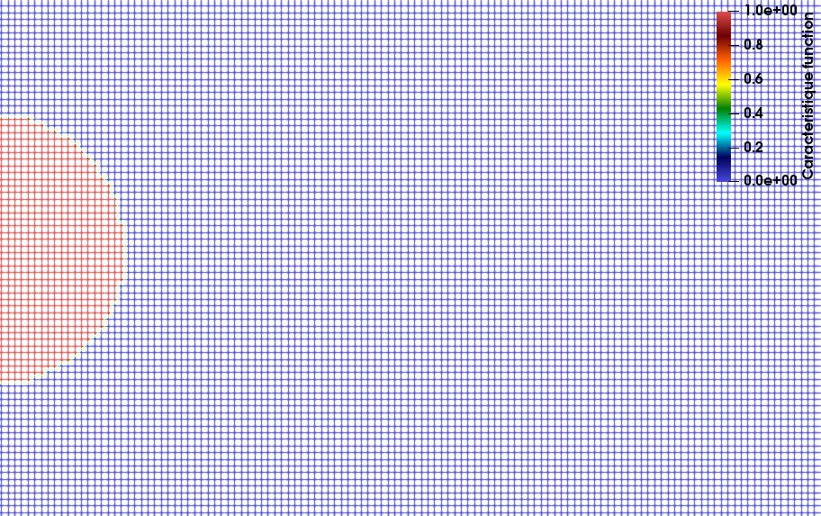
(b) Characteristic function used for the VP-LBM

Figure 4: Grids used for the finite volume computations and for the VP-LBM computations

For the computation performed with Code$\_$Saturne, a non uniform grid that was very fine in the vicinity of the cylinder, and coarser in the remaining of the fluid domain, was built (see figure 4(a)). Such a mesh enabled a decrease in computational time. For the LBM computations, a regular grid was used.

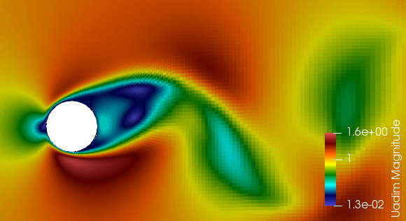
(a) $\|\mathbf{u}^{\star}\|$ Code$\_$Saturne

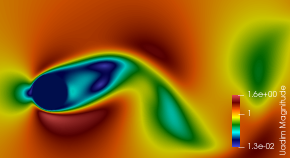
(b) $\|\mathbf{u}^{\star}\|$ VP-LBM

Figure 5: Non-dimensional velocity fields obtained with Code$\_Saturne$, and with the VP-LBM computations, for the imposed motion of a cylinder

Figure 5 shows the norms of the non-dimensional velocity field computed with Code$\_$Saturne software and with the VP-LBM at the same non-dimensional time $t^{\star}=64$, where $t^{\star}=t\dfrac{U_{0}}{D}$. It can bee seen that both computations yield the same velocity field. More particularly, the vortex which appears behind the moving cylinder is located at the same place.

In figures 6, the lift $\left(C_{L}\right)$ and drag $\left(C_{D}\right)$ coefficients are compared :

$$C_{L}=\dfrac{\boldsymbol{\mathcal{F}_{f}}\cdot\mathbf{y}}{\dfrac{1}{2}\rho D\left(U_{0}\right)^{2}}\hskip 28.45274ptC_{D}=\dfrac{\boldsymbol{\mathcal{F}_{f}}\cdot\mathbf{x}}{\dfrac{1}{2}\rho D\left(U_{0}\right)^{2}}$$

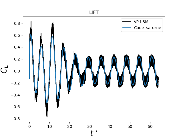
(a) $C_{L}$

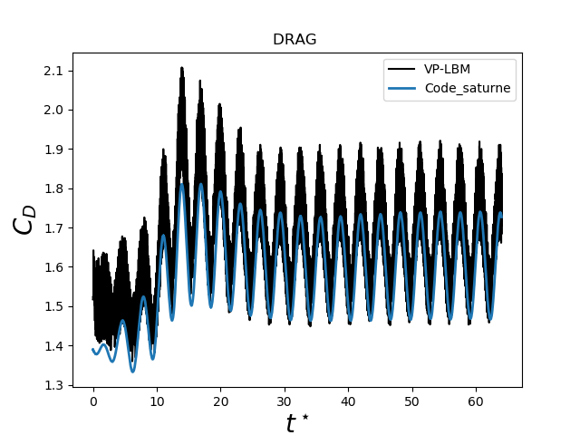
(b) $C_{D}$

Figure 6: Comparison of $C_{L}$ and $C_{D}$ obtained with the VP-LBM and Code$\_$Saturne

In this figure, it can be noticed that spurious oscillations occur when LBM is used. However, when using LBM, a cartesian grid is commonly used, and this behavior has been highlighted for computations of FSI problems carried out with LBM, combined with any method chosen for simulating flows around curved boundaries (Bounce-back or immersed boundary methods) ([20]). A good agreement between both methods was obtained for the lift coefficient, whereas small differences are observed for the drag coefficient. These differences are not discriminating for the VP-LBM approach, because as shown in table 1, the difference based on the average drag is less than $5\%$, and this gap is in the range of what can be expected when two different numerical models are compared.

•	VP-LBM	Code_Saturne
$\overline{C_{D}}$	1.653	1.577

Table 1: Average drag coefficient obtained with the VP-LBM and Code$\_$Saturne

To conclude with this first example, the VP-LBM predicts accurately the fluid forces exerted on a solid whose motion is imposed. In order to test the validity of the VP-LB, the following examples deal with real cases of fluid structure interaction.

Remark

In order to reduce the size of the LBM problem ($L_{1}\times L_{2}$) and thus the computational time, the value of the parameter $\tau=0.56$ was chosen very close to the stability limit $0.5$. An inlet velocity of $0.048780$ ensured a small Mach number suitable for the LBM approach. For that simulation, $41$ lattice units were used for the cylinder diameter, which is a small value for computing a flow of Reynolds number $100$ with LBM. This can explain the spurious oscillations.

3.2 Sedimentation of a particle under gravity

The next case focuses on the sedimentation of a particle under gravity in an infinite channel (figure 7) for centered and non-centered configurations. These problems have been extensively used for model validations and are very useful to test the capacity of a method to capture complex trajectories [24, 25, 20].

Figure 7: Schematic description of particle sedimentation

A circular particle of diameter $D$ falls under gravity $\boldsymbol{g}$ in a fluid of density $\rho$ in a vertical channel of width $H$. At the initial state, the particle is at a distance $x_{0}$ from the left wall, a distance $y_{0}$ from the top of the channel and the velocity of the particle is equal to zero. For that case, the particle displacement can be described using equations (23 ) and (24) modified as follows :

$$m\dfrac{d^{2}\boldsymbol{x_{G}}}{dt^{2}} = \boldsymbol{\mathcal{F}_{f}}+m\left(1-\dfrac{\rho}{\rho_{s}}\right)\boldsymbol{g}$$ (31)

$$I\dfrac{d^{2}\boldsymbol{\theta}}{dt^{2}} = \boldsymbol{\mathcal{T}_{f}}$$ (32)

where $\rho$ denotes the fluid density and $\rho_{s}$ the solid density. The last term in equation (31) represents the weight and the buoyancy (Archimedes’ principle) acting on the particle.

For small Reynolds numbers and a large non dimensional width $\tilde{H}=\dfrac{H}{D}$, the particle reaches a steady state, where the drag force can be approximated according to the following expression [26]:

$$\mathcal{F}_{D}=\dfrac{1}{4}\pi D^{2}\left(\rho_{p}-\rho_{f}\right)=4\pi\kappa\mu\mathbf{v_{s}}\cdot\mathbf{y}$$ (33)

where $\kappa$ denotes the correction factor which represents the channel confinement effect,

$$\kappa=\displaystyle\left(\textrm{ln}\tilde{H}-0.9157+1.7244\tilde{H}^{-2}-1.7302\tilde{H}^{-4}+2.4056\tilde{H}^{-6}-4.5913\tilde{H}^{-8}\right)^{-1}$$ (34)

$\mu$ is the fluid viscosity and $\mathbf{v_{s}}$ is the gravitational settling of the particle :

$$\mathbf{v_{s}}=\dfrac{D^{2}}{16\kappa\mu}\left(\rho-\rho_{s}\right)\boldsymbol{g}$$ (35)

3.2.1 Centered particle : $x_{0}=\dfrac{H}{2}$

We consider the same physical properties as those chosen in previous works [24, 27]. The diameter of the particle is $D=0.24\;\textrm{cm}$, the fluid density is $\rho=1\;\textrm{g}\cdot\textrm{cm}^{-3}$, the fluid viscosity is $\mu=0.1\;\textrm{g}\cdot\textrm{cm}^{-1}\cdot\textrm{s}^{-1}$, the gravitational acceleration is $\|\boldsymbol{g}\|=980\;\textrm{cm}\cdot\textrm{s}^{-2}$ and the non dimensional width of the channel is $\tilde{H}=5$.

The problem was modelled with a regular $120\times 1200$ lattice grid, $24$ nodes across the diameter of the cylinder ($D_{LBM}=24\;\textrm{l.u.}$), and a relaxation time $\tau=0.8$. Initially, the particle is located at the center of the channel : $x_{0}=0.5H$ and $y_{0}=0.5L$. No-slip boundary conditions were imposed on the left and right walls. A zero velocity boundary condition was applied at the inlet (top of the channel) and free stream conditions were applied at the outlet (bottom). A large value of $L$ was chosen, so that the inlet and outlet did not influence the behavior of the particle.

Computations were performed for various mass ratios $\rho_{r}=\dfrac{\rho_{s}}{\rho}$ taken from the following list :

$$0.95;0.98;0.99;1.01;1.02;1.05$$ (36)

For all cases the particle velocities and the drag coefficients are plotted in figure 8 and compared with the analytical solution (equations (33) and (35)).

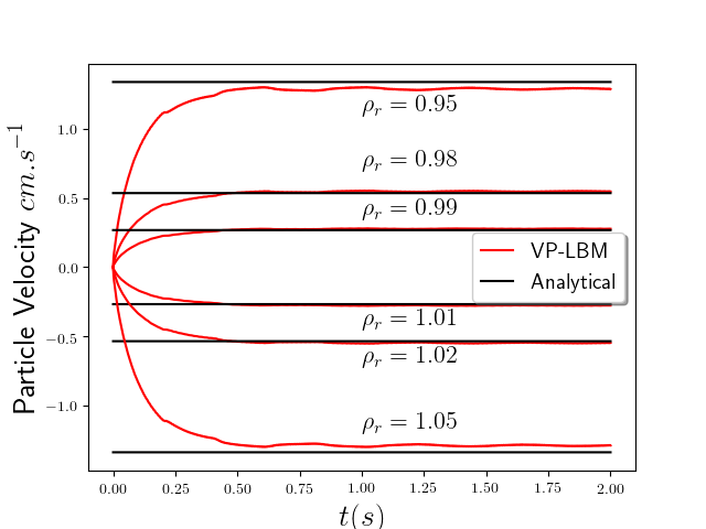
(a) Particle velocities

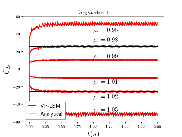
(b) Drag coefficients

Figure 8: Comparison of particle velocities and drag coefficients for different mass ratios (Centered particle and $\tilde{H}=5$)

For $\rho_{r}=\left\{0.98;0.99;1.01;1.02\right\}$, results match with the analytical solution. For larger ratios ($\rho_{r}=\left\{0.95;1.05\right\}$) differences are observed. As mentioned in previous studies [25, 27], the reason could be that the analytical solutions are available only for small mass numbers $\rho_{r}$ and not for larger ratios such as $1.05$ or $0.95$, which explains the gap between the analytical solution and the results obtained with the VP-LBM approach. As noticed in the previous example, small fluctuations on the drag coefficient are observed when the velocity increases $\left(\rho_{r}=0.95\;\textrm{or}\;1.05\right)$, but the averages fit with the analytical solutions.

3.2.2 Non centered particle : $x_{0}=0.75D$

The following case deals with a particle whose initial position is not at the center of the channel. The fluid properties are $\rho=1\;\textrm{g}\cdot\textrm{cm}^{-3}$, and $\mu=0.1\;\textrm{g}\cdot\textrm{cm}^{-1}\cdot\textrm{s}^{-1}$ and the physical problem concerns a particle of diameter $D=0.1\;\textrm{cm}$, a mass ratio $\rho_{r}=1.03$ and $\|\boldsymbol{g}\|=980\;\textrm{cm}\cdot\textrm{s}^{-2}$. The Reynolds number based on the final velocity of the particle is $Re=8.33$.

For the LBM computations a $125\times 1550$ lattice grid was used, the cylinder diameter was $31\;\textrm{l.u.}$, the non dimensional relaxation time was $\tau=0.6$ and the particle was released at $y_{0}=12.5D$. The boundary conditions were the same as in the previous case.

Results are plotted in figures 9. $\mathbf{v_{g}}$ denotes the vector velocity of the gravity center of the particle, and $\omega_{g}$ its rotational velocity. The time-dependent position, horizontal, vertical and rotational velocities are compared with results from Tao et al. [25] and good agreements are found between them. Small spurious oscillations are observed for the rotational velocity (figure 9(d)), but these oscillations are also observed by Tao et al. [25].

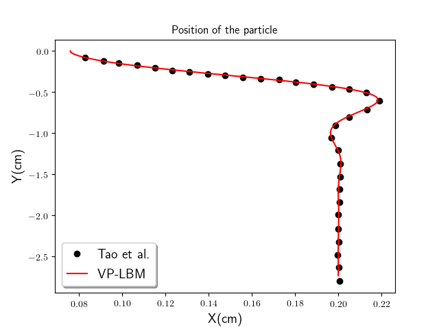
(a) position of the particle

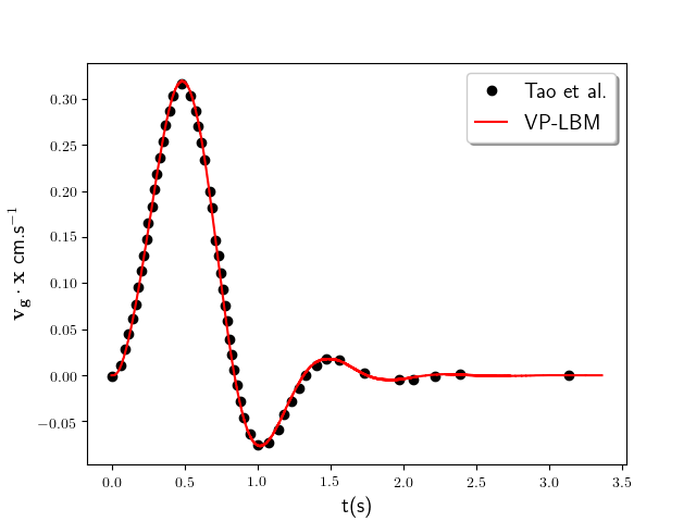
(b) horizontal velocity

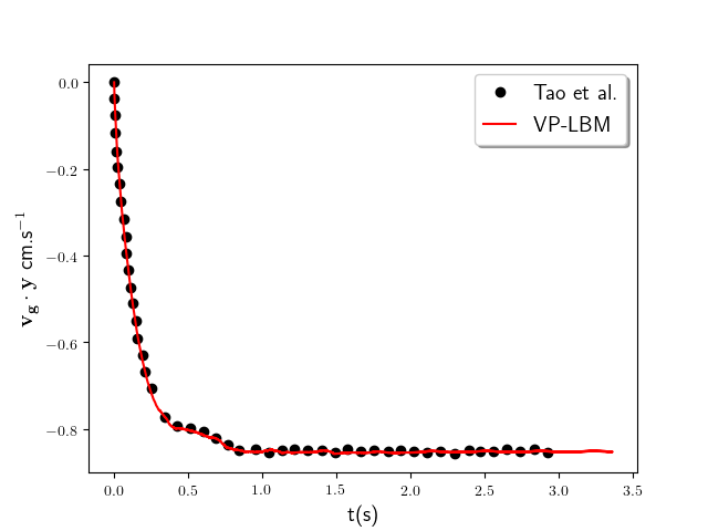
(c) vertical velocity

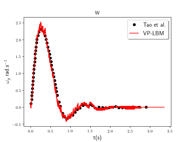
(d) rotational velocity

Figure 9: Results obtained using the VP-LBM apporach and compared with Tao et al’s results [25]

Figures 10 and 11 show the fluid velocity and the vorticity field around the particle at four different times. The dynamics of the flow field and the particle can be analyzed using the velocity magnitude and the vorticity. The particle goes first to the right and rotates in a positive direction. Next a brief oscillation occurs around the central line of the channel and finally the particle stays in the middle of the channel with a steady velocity.

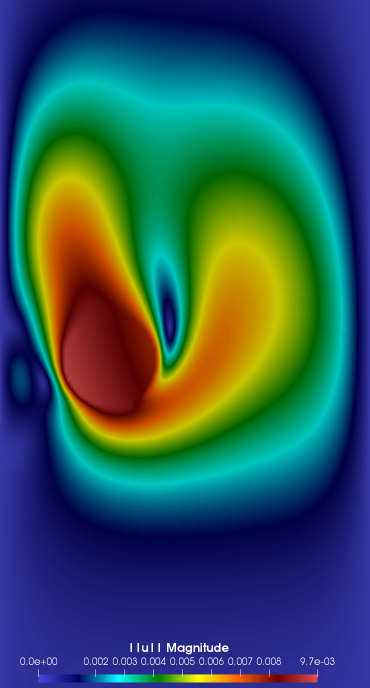
(a) t = 0.4 s

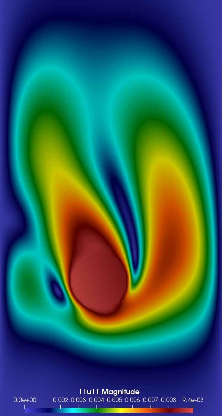
(b) t = 0.6 s

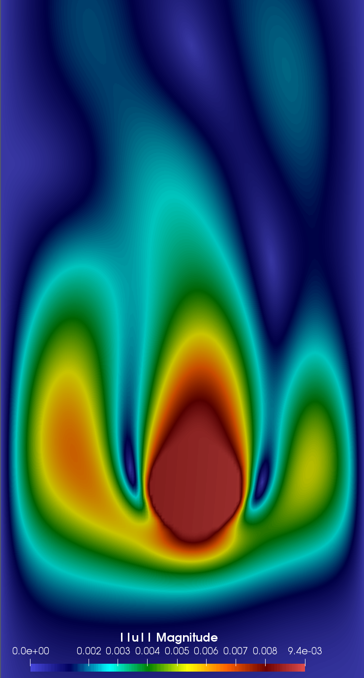
(c) t = 1.0 s

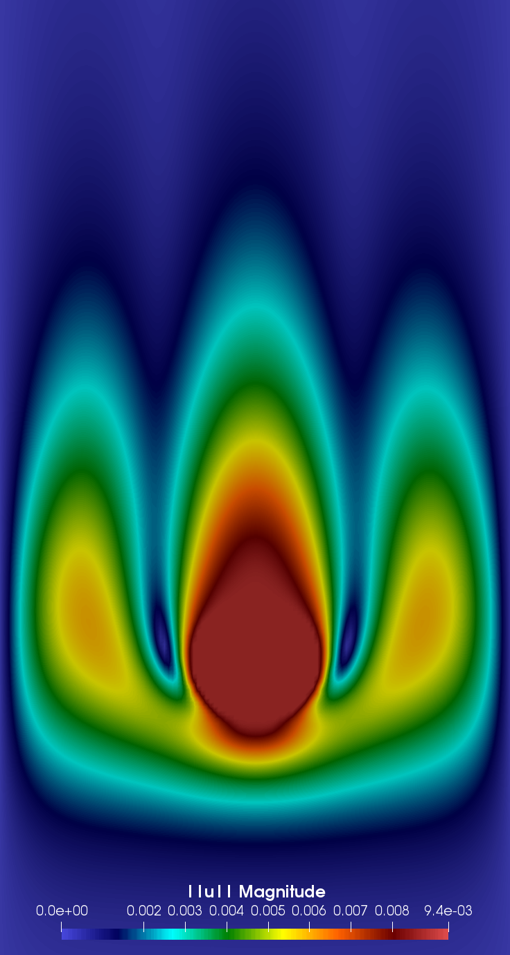
(d) t = 3.0 s

Figure 10: Fluid velocity magnitude at times t=0.4, 06, 1.0 and 3.0 seconds in lattice units

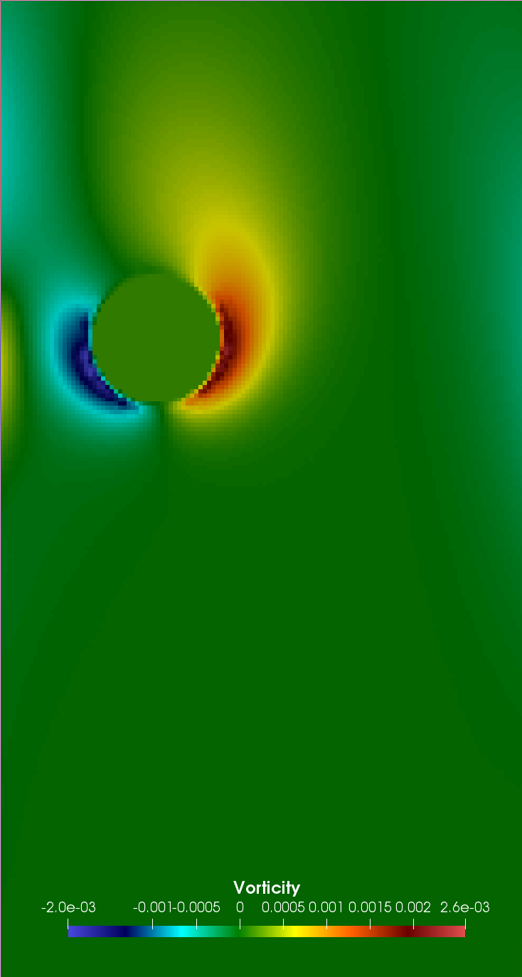
(a) t = 0.4 s

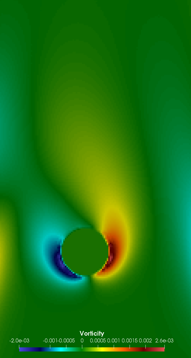
(b) t = 0.6 s

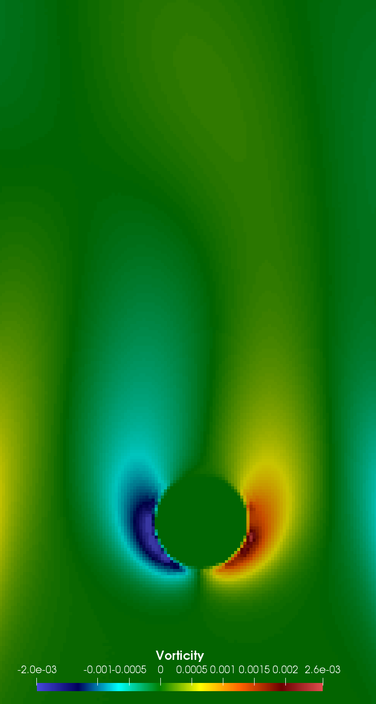
(c) t = 1.0 s

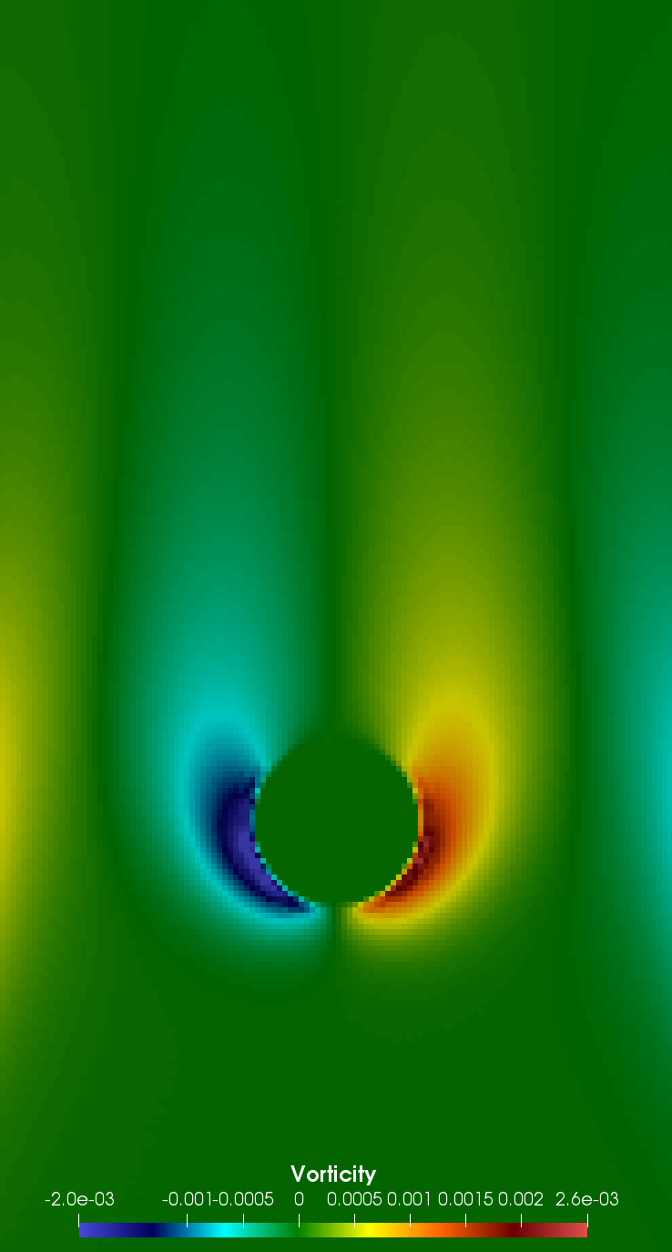
(d) t = 3.0 s

Figure 11: Fluid vorticity at times t=0.4, 06, 1.0 and 3.0 seconds in lattice units

This example shows that the VP-LBM method is able to predict a complex trajectory for a real case of fluid structure interaction at a very low Reynolds number.

3.3 Vortex Induced Vibration of a cylinder

Let us consider the case depicted in figure 3. In this paragraph the displacement of the cylinder is not imposed, but driven by the fluid forces. The displacement is let free according to the $\mathbf{y}$ axis. Initially, the cylinder is at rest, the force exerted by the spring on the cylinder is equal to $0$. Due to the vortex shedding, the fluid applies a force according to the vertical axis and the cylinder begins to oscillate. The rigid displacement of the cylinder is solved using equation (23) projected onto the $\mathbf{y}$ axis, with $c=0$ and $\boldsymbol{\mathcal{F}_{ext}}=0$ :

$$m\ddot{y}_{G}+k\left(y_{G}-y_{0}\right)=\mathcal{F}_{y}$$ (37)

where $y_{G}$ is the position of the center of gravity of the cylinder according to the $\mathbf{y}$ axis, $y_{0}$ is the position at rest, and $\mathcal{F}_{y}$ denotes the fluid forces acting on the cylinder in the vertical direction. Equation (24) is not used.

To simplify the analysis, the non dimensional form of equation (37) is considered :

$$m^{\ast}\ddot{y}^{\ast}+k^{\ast}\left(y^{\ast}-y^{\ast}_{0}\right)=C_{L}$$ (38)

with the non dimensional numbers :

$$m^{\ast}=\dfrac{m}{0.5\rho D^{2}}\hskip 14.22636ptk^{\ast}=\dfrac{k}{0.5\rho U^{2}_{0}}\hskip 14.22636pty^{\ast}=\dfrac{y_{G}}{D}\hskip 14.22636ptC_{L}=\displaystyle\dfrac{\mathcal{F}_{y}}{\dfrac{1}{2}\rho U^{2}_{0}D}\hskip 14.22636ptt^{\ast}=t\dfrac{U_{0}}{D}$$

To scale the results, the effective stiffness introduced by Shiels et al. [28] is used :

$$k^{\ast}_{\textrm{eff}}=k^{\ast}-m^{\ast}{\omega^{\ast}}^{2}$$ (39)

where $\omega^{\ast}$ is computed from the analysis of the cylinder displacement. The effective stiffness enables to use only one plot to represent the results, because it combines the reduced mass $m^{\ast}$ and the reduced stiffness $k^{\ast}$. For a given Reynolds number, $k^{\ast}_{\textrm{eff}}$ completely determines the system.

The computational parameters are identical to those related to the first test case (section 3.1)

$$\tau=0.56\hskip 14.22636ptU_{0}=0.048780\;\textrm{l.u.}\hskip 14.22636ptL_{1}=1230\;\textrm{l.u.}\hskip 14.22636ptL_{2}=410\;\textrm{l.u.}\hskip 14.22636ptD=41\;\textrm{l.u.}$$

$29$ values of the stiffness parameter $k^{\ast}$ were considered, from $1$ to $30$. For each $k^{\ast}$, the choice of $\omega^{\ast}$ was based on the the analysis of the drag coefficient, and with these values, $k^{\ast}_{\textrm{eff}}$ was computed.

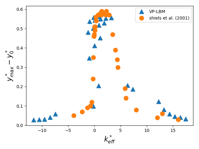
Figure 12: Results obtained using the VP-LBM and compared with Shiels et al.’s results [28]

In figure 12 the maximum of the non dimensional amplitude $y^{\ast}_{max}-y^{\ast}_{0}$ versus $k^{\ast}_{\textrm{eff}}$, obtained obtained by the VP-LBM methods and compared with data from [28] is plotted. It can be seen that the proposed method is able to reproduce the lock-in phenomena when $k^{\ast}$ is close to $m{\omega^{\ast}}^{2}$, and when important displacement of the cylinder occurs (more than $50\%$ of the diameter). Figure 13 depicts the temporal evolution of the non-dimensional amplitude for $3$ values of $k^{\ast}$. The velocity, pressure and vorticity fields are presented in figures 14-16. Different behaviors according to the value of $k^{\ast}$ were obtained. For high values of $k^{\ast}$ the displacement of the cylinder is small, and the fluid flow shows similar features as seen for a fixed cylinder. However, the behavior of the solid is more chaotic, several frequencies can be noticed when examining the displacement of the body (figure 13(c)). For $1\leq k^{\ast}_{eff}\leq 5$ the flow pattern changes drastically. The vortex shedding frequency increases and the velocity decreases in the wake of the cylinder (figure 14(b)).

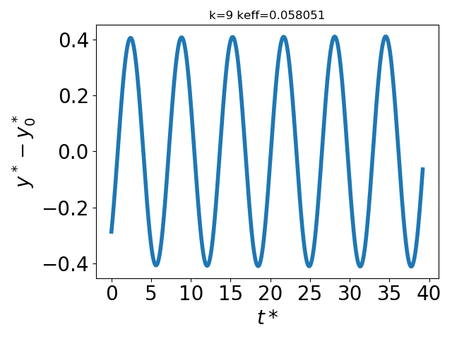
(a) $k^{\ast}=9\;k^{\ast}_{\textrm{eff}}=0.058$

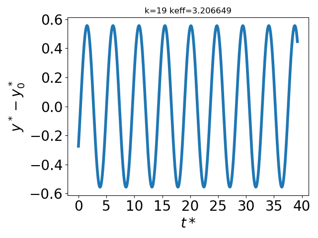
(b) $k^{\ast}=19\;k^{\ast}_{\textrm{eff}}=3.20$

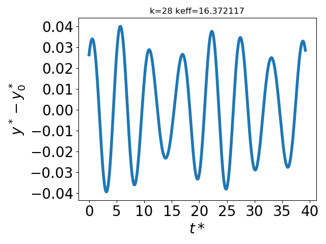
(c) $k^{\ast}=28\;k^{\ast}_{\textrm{eff}}=16.37$

Figure 13: Time-dependent value of the non dimensional amplitude $y^{\ast}-y^{\ast}_{0}$ for 3 values of $k^{\ast}$

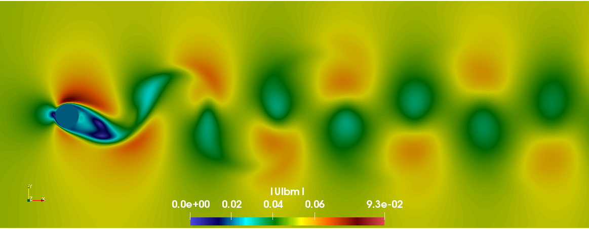
(a) $k^{\ast}=9\;k^{\ast}_{\textrm{eff}}=0.058$

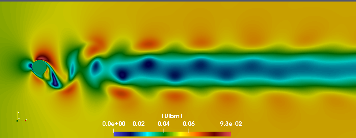
(b) $k^{\ast}=19\;k^{\ast}_{\textrm{eff}}=3.20$

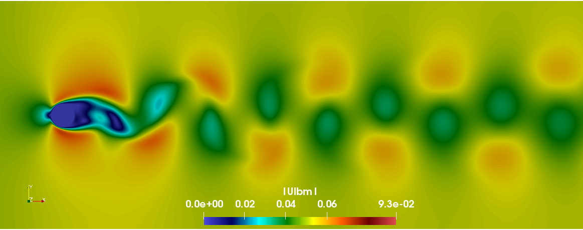
(c) $k^{\ast}=28\;k^{\ast}_{\textrm{eff}}=16.37$

Figure 14: Field of velocity magnitude in lattice units for 3 values of $k^{\ast}$

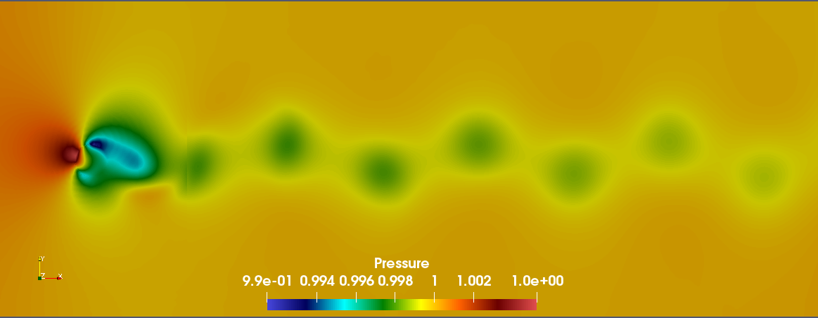
(a) $k^{\ast}=9\;k^{\ast}_{\textrm{eff}}=0.058$

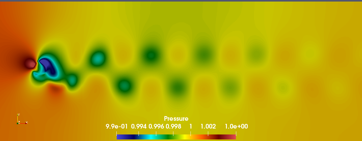
(b) $k^{\ast}=19\;k^{\ast}_{\textrm{eff}}=3.20$

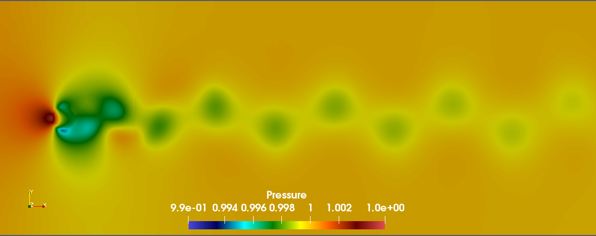
(c) $k^{\ast}=28\;k^{\ast}_{\textrm{eff}}=16.37$

Figure 15: Pressure field in lattice units for 3 values of $k^{\ast}$

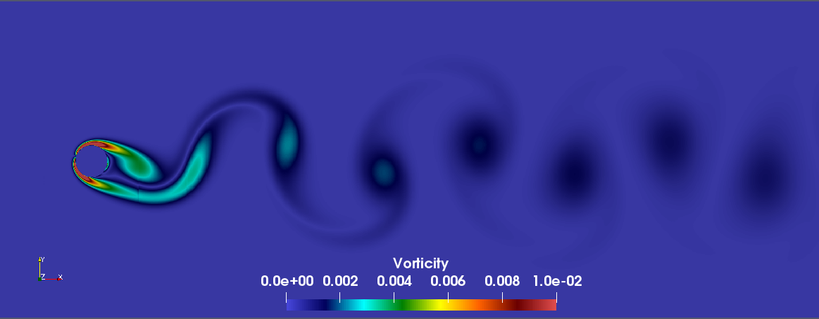
(a) $k^{\ast}=9\;k^{\ast}_{\textrm{eff}}=0.058$

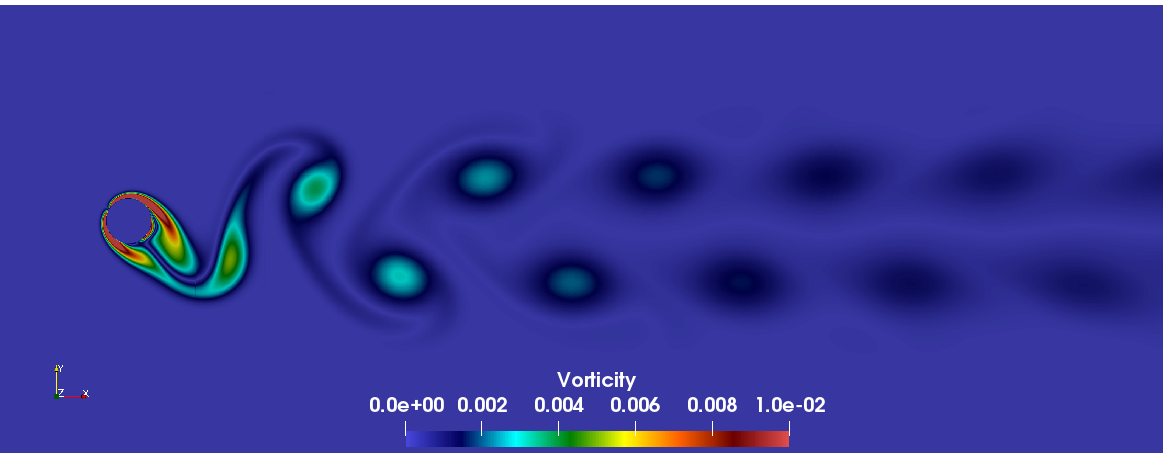
(b) $k^{\ast}=19\;k^{\ast}_{\textrm{eff}}=3.20$

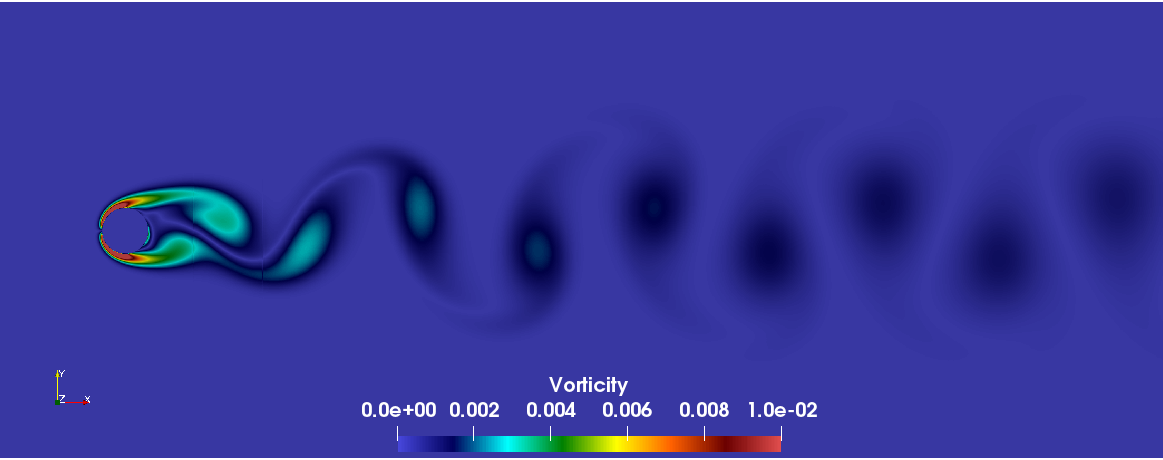
(c) $k^{\ast}=28\;k^{\ast}_{\textrm{eff}}=16.37$

Figure 16: Vorticity field in lattice units for 3 values of $k^{\ast}$

To conclude, this last application shows the capacity of the VP-LBM method to capture various physical behaviors induced by changes of the parameter $k^{\ast}$.

4 Conclusion

A combined approach coupling the Volume Penalization and the Lattice Boltzmann method for fluid structure interaction was proposed. The method consists in adding a force term, which is similar to Darcy’s law, into the Boltzmann equation. The advantage of this method is that no explicit computation of the fluid structure interface is needed, the use of a characteristic function is sufficient. In addition, the fluid forces exerted on the structure are computed using the classical momentum exchange method. The method was implemented on a GPU architecture device and tested on three cases. The first case which deals with the imposed displacement of a cylinder in a transverse fluid flow at a Reynolds of $100$, validates the capacity of the method to compute drag and lift forces. The second application focuses on the sedimentation of a particle at a very low Reynolds number in a channel. The proposed method succeeds to capture the complex trajectory of the particle, which is composed of translational and rotational components. In the last application, the vortex induced vibration of a cylinder in a transverse fluid flow is considered. The capacity of the method to predict the physics of the fluid flow and the structure behavior for different values of the stiffness parameter of the cylinder is tested. Results are in a good agreement with those of literature. All these applications validate the VP-LBM as an efficient tool to model FSI in case of rigid bodies.

5 Bibliography

References

- [1] R. Benzi, S. Succi, M. Vergassola, The lattice Boltzmann equation: theory and applications, Physics Reports 222 (3) (1992) 145–197. doi:10.1016/0370-1573(92)90090-M.
- [2] Z. Fan, F. Qiu, A. Kaufman, S. Yoakum-Stover, GPU cluster for high performance computing, IEEE/ACM SC2004 Conference, Proceedings (2004) 297–308.
- [3] T. Kruger, H. Kusumaatmaja, A. Kuzmin, O. Shardt, G. Silva, E. M. Viggen, The Lattice Boltzmann Method - Principles and Practice, Graduate Texts in Physics, Springer International Publishing, 2017. doi:10.1007/978-3-319-44649-3.
- [4] A. Ladd, R. Verberg, Lattice-Boltzmann simulations of particle-fluid suspensions, Journal of Statistical Physics 104 (5-6) (2001) 1191–1251. doi:10.1023/A:1010414013942.
- [5] D. Yu, R. Mei, W. Shyy, A unified boundary treatment in lattice Boltzmann method. 41st aerospace sciences meeting and exhibit, vol. 1, AIAA (2003) 2003–2953doi:10.2514/6.2003-953.
- [6] M. Bouzidi, M. Firdaouss, P. Lallemand, Momentum transfer of a Boltzmann-lattice fluid with boundaries, Physics of Fluids 13 (11) (2001) 3452–3459. doi:10.1063/1.1399290.
- [7] D. Noble, J. Torczynski, A lattice-Boltzmann method for partially saturated computational cells, International Journal of Modern Physics C 9 (8) (1998) 1189–1201. doi:10.1142/S0129183198001084.
- [8] Z.-G. Feng, E. Michaelides, The immersed boundary-lattice Boltzmann method for solving fluid-particles interaction problems, Journal of Computational Physics 195 (2) (2004) 602–628. doi:10.1016/j.jcp.2003.10.013.
- [9] A. Dupuis, P. Chatelain, P. Koumoutsakos, An immersed boundary-lattice-Boltzmann method for the simulation of the flow past an impulsively started cylinder, Journal of Computational Physics 227 (9) (2008) 4486–4498. doi:10.1016/j.jcp.2008.01.009.
- [10] Y. Wang, C. Shu, C. Teo, J. Wu, An immersed boundary-lattice Boltzmann flux solver and its applications to fluid structure interaction problems, Journal of Fluids and Structures 54 (2015) 440 – 465. doi:10.1016/j.jfluidstructs.2014.12.003.
- [11] P. Angot, C.-H. Bruneau, P. Fabrie, A penalization method to take into account obstacles in incompressible viscous flows, Numerische Mathematik 81 (4) (1999) 497–520. doi:10.1007/s002110050401.
- [12] M. Benamour, E. Liberge, C. Béghein, Lattice Boltzmann method for fluid flow around bodies using volume penalization, International Journal of Multiphysics 9 (3) (2015) 299–315. doi:10.1260/1750-9548.9.3.299.
- [13] M. Benamour, E. Liberge, C. Béghein, A new approach using lattice Boltzmann method to simulate fluid structure interaction, Energy Procedia 139 (2017) 481–486. doi:10.1016/j.egypro.2017.11.241.
- [14] B. Kadoch, D. Kolomenskiy, P. Angot, K. Schneider, A volume penalization method for incompressible flows and scalar advection-diffusion with moving obstacles, Journal of Computational Physics 231 (12) (2012) 4365–4383. doi:10.1016/j.jcp.2012.01.036.
- [15] P. Bhatnagar, E. Gross, M. Krook, A model for collision processes in gases. I. Small amplitude processes in charged and neutral one-component systems, Physical Review 94 (3) (1954) 511–525. doi:10.1103/PhysRev.94.511.
- [16] D. d’Humière, Rarefied Gas Dynamics: Theory and Simulations, Progress in Astronautics and Aeronautics, 1992, Ch. Generalized Lattice-Boltzmann Equations, pp. 450–458. doi:10.2514/5.9781600866319.0450.0458.
- [17] J. Lu, H. Han, B. Shi, Z. Guo, Immersed boundary lattice Boltzmann model based on multiple relaxation times, Physical Review E - Statistical, Nonlinear, and Soft Matter Physics 85 (1). doi:10.1103/PhysRevE.85.016711.
- [18] D. Yu, R. Mei, L.-S. Luo, W. Shyy, Viscous flow computations with the method of lattice Boltzmann equation, Progress in Aerospace Sciences 39 (5) (2003) 329–367. doi:10.1016/S0376-0421(03)00003-4.
- [19] Z. Guo, C. Zheng, B. Shi, Discrete lattice effects on the forcing term in the lattice Boltzmann method, Physical Review E 65 (4) (2002) 046308. doi:10.1103/PhysRevE.65.046308.
- [20] B. Wen, C. Zhang, Y. Tu, C. Wang, H. Fang, Galilean invariant fluid–solid interfacial dynamics in lattice Boltzmann simulations, Journal of Computational Physics 266 (2014) 161 – 170. doi:10.1016/j.jcp.2014.02.018.
- [21] J. P. Giovacchini, O. E. Ortiz, Flow force and torque on submerged bodies in lattice-Boltzmann methods via momentum exchange, Phys. Rev. E 92 (2015) 063302. doi:10.1103/PhysRevE.92.063302.
- [22] F. Archambeau, N. Méchitoua, S. M., Code_saturne : a finite volume code for the computation of turbulent incompressible flows, International Journal on Finite Volumes 1.
- [23] Z. Yang, Lattice Boltzmann outflow treatments: Convective conditions and others, Computers and Mathematics with Applications 65 (2) (2013) 160–171. doi:10.1016/j.camwa.2012.11.012.
- [24] L. Wang, Z. Guo, B. Shi, C. Zheng, Evaluation of three lattice Boltzmann models for particulate flows, Communications in Computational Physics 13 (4) (2013) 1151–1171. doi:10.4208/cicp.160911.200412a.
- [25] S. Tao, J. Hu, Z. Guo, An investigation on momentum exchange methods and refilling algorithms for lattice Boltzmann simulation of particulate flows, Computers and Fluids 133 (2016) 1–14. doi:10.1016/j.compfluid.2016.04.009.
- [26] J. Happel, H. Brenner, Low Reynolds number hydrodynamics, Springer Netherlands, 1983. doi:10.1007/978-94-009-8352-6.
- [27] B. Dorschner, S. Chikatamarla, F. Bösch, I. Karlin, Grad’s approximation for moving and stationary walls in entropic lattice Boltzmann simulations, Journal of Computational Physics 295 (2015) 340–354. doi:10.1016/j.jcp.2015.04.017.
- [28] D. Shiels, A. Leonard, A. Roshko, Flow-induced vibration of a circular cylinder at limiting structural parameters, Journal of Fluids and Structures 15 (1) (2001) 3–21. doi:10.1006/jfls.2000.0330.