A sharp critical threshold for a traffic flow model with look-ahead dynamics

Abstract.

We study a nonlocal traffic flow model with an Arrhenius type look-ahead interaction. We show a sharp critical threshold condition on the initial data which distinguishes the global smooth solutions and finite time wave break-down.

1. Introduction

We consider the following one-dimensional traffic flow model with a nonlocal flux

$$\begin{cases}\partial_{t}u+\partial_{x}\big{(}u(1-u)e^{-\bar{u}}\big{)}=0,&t>0,x\in\mathbb{R},\\ u(0,x)=u_{0}(x),&x\in\mathbb{R}.\end{cases}$$ (1)

Here, $u(t,x)$ represents the vechicle density normalized in the interval $[0,1]$. The velocity of the flow $v=(1-u)e^{-\bar{u}}$ becomes zero when the maximum density is reached. It is also weighted by a nonlocal Arrhenius type slow down factor $e^{-\bar{u}}$, where

$$\bar{u}(t,x)=(K*u)(t,x)=\int_{\mathbb{R}}K(x-y)u(t,y)\,dy,$$ (2)

with appropriately choices of the kernel $K$ to be discussed later.

We are interested in the local and global wellposedness of this nonlocal macroscopic traffic flow model (1)-(2). The goal is to understand whether smooth solutions presist in all time, or there is a finite time singularity formation. Such blowup is known as the wave break-down phenomenon, which discribes the generation of the traffic jam.

1.1. Nonlocal conservation laws

The traffic flow model (1) falls into a class of models in nonlocal scaler conservation laws, which has the form

$$\partial_{t}u+\partial_{x}F(u,\bar{u})=0,$$ (3)

where the flux $F$ depends on both the local density $u$, and the nonlocal quantity $\bar{u}$ defined in (2). This class of models has a variety of applications, not only in traffic flows [16, 21, 24], but also in dispersive water waves [9, 12, 23, 30], the collective motion of biological cells [5, 10], high-frequency waves in relaxing medium [13, 29], the kinematic sedimentation [4, 17, 31], and many more. The understanding of the wave break-down phenomenon is important and challenging for these models.

Here are several intriguing models that lie in this class (3).

• The Whitham equation in nonlinear water waves [30]

  $$\partial_{t}u+\partial_{x}\left(\alpha u^{2}+\bar{u}\right)=0,$$

  where the kernel has its Fourier transform $\hat{K}(\xi)=\left(\frac{\tanh\xi}{\xi}\right)^{1/2}$. Wave break-down has been shown in [14], for initial conditions which are near break-down.

• A one-dimensional hyperbolic Keller-Segel model [10]

  $$\partial_{t}u+\partial_{x}\left(u(1-u)\partial_{x}S\right)=0,\quad-\partial_{xx}^{2}S+S=u.$$

  It is shown in [20] that wave break-down happens for a set of supercritical initial conditions.

• The one-dimensional aggregation equation

  $$\partial_{t}u+\partial_{x}\left(u\bar{u}\right)=0,$$

  where the kernel $K=-\partial_{x}\phi$ for some interaction potential $\phi$. If $\phi$ is attractive, then the solution is globally regular if and only if the Osgood condition holds [2, 3, 7]. There will be finite time density consentration if the condition is violated. For general attractive-repulsive interaction potential, there will be no density concentration if the repulsion is strong enough. However, there might be wave break-down in finite time, see for instance [27].

The wave break-down phenomenon for general nonlocal conservation laws (3) has been recently studied in [18]. A sufficient condition on initial data is derived which guarantees a finite time blowup.

1.2. Nonlocal traffic models

We focus on the nonlocal traffic models (1)-(2). It is another example of the nonlocal conservation law (3).

When there is no interaction, namely $K\equiv 0$, the dynamics is the classical Lighthill-Whitham-Richards (LWR) model

$$\partial_{t}u+\partial_{x}(u(1-u))=0.$$ (4)

For this local model, it is well-known that there is a finite time wave break-down for any smooth initial data.

For uniform interaction $K\equiv 1$, the nonlocal term

$$\bar{u}(t,x)=\int_{\mathbb{R}}u(t,y)dy=\int_{\mathbb{R}}u_{0}(y)dy=:m$$

is a constant, due to the conservation of mass. Then, the dynamics again becomes LWR model, with velocity $v=(1-u)e^{-m}$.

Another class of choices of $K$ is called the look-ahead kernel, where

$$\text{supp}(K)\subseteq(-\infty,0].$$

Under the assumption, the nonlocal term

$$\bar{u}(t,x)=\int_{x}^{\infty}K(x-y)u(t,y)dy$$

only depends on the density ahead. Sopasakis and Katsoulakis (SK) in [24] introduce a celebrated traffic model with Arrhenius type look-ahead interactions, where

$$K(x)=\begin{cases}1&-1<x<0,\\ 0&\text{otherwise}.\end{cases}$$ (5)

A family of kernel with look-ahead distance $L$ can be generated by the scaling

$$K_{L}(x)=K\left(\frac{x}{L}\right).$$ (6)

Note that when taking $L\to 0$, the system reduces to the local LWR model (4).

The wave break-down phenomenon for the SK model is observed in [16], through an extensive numerical study. A different class of linear look-ahead kernel is also introduced, with

$$K(x)=\begin{cases}2\big{(}1-(-x)\big{)}&-1<x<0,\\ 0&\text{otherwise}.\end{cases}$$ (7)

Numerical examples suggest that wave break-down happens in finite time, for a class of initial data. However, unlike the LWR model, it is generally unclear for the nonlocal models whether wave break-down happens for all smooth initial data.

1.3. Critical threshold and wave break-down

In many examples above, whether there is a finite time wave break-down depends on the choice of initial conditions: subcritical initial data lead to global smooth solution, while supercritical initial data lead to a finite time wave break-down. This is known as the critical threshold phenomenon, which has been studied in the context of Eulerian dynamics, including the Euler-Poisson equations [11, 19, 25], the Euler-Alignment equations [6, 26, 28], and more systems of conservation laws.

A critical threshold is called sharp if all initial data lie in either the subcritical region, or the supercritical region.

For the traffic model (1) with nonlocal look-ahead interactions (5) or (7), a supercritical region has been obtained in [21]. which leads to a finite time wave break-down. However, the result is not sharp. In particular, a challenging open question is, whether there exists subcritical initial data, such that the solution is globally regular.

1.4. Main result

We study the traffic flow model (1) with the following look-ahead interaction

$$K(x)=\begin{cases}1&-\infty<x<0,\\ 0&\text{otherwise}.\end{cases}$$ (8)

The kernel can be viewed as a limit of the SK model (5) under scaling (6), with look-ahead distance $L\to\infty$.

The corresponding nonlocal term is given by

$$\bar{u}(t,x)=\int_{x}^{\infty}u(t,y)dy.$$ (9)

The main result is stated as follow:

Theorem 1.1 (Sharp critical threshold).

Consider the traffic flow model (1) with a nonlocal look-ahead kernel (9). Suppose the initial data is smooth, with $u_{0}\in L^{1}\cap H^{s}(\mathbb{R})$ for $s>3/2$, and $0\leq u_{0}\leq 1$. Let $\sigma$ be a function defined in (24). Then,

• If the initial data is subcritical, satisfying

  $$u_{0}^{\prime}(x)\leq\sigma(u_{0}(x)),\quad\forall~{}x\in\mathbb{R},$$ (10)

  then the solution exists globally in time. Namely, for any $T>0$, there exists a unique solution $u\in C([0,T];L^{1}\cap H^{s}(\mathbb{R}))$.

• If the initial data is supercritical, satisfying

  $$\exists~{}x_{0}\in\mathbb{R}\quad s.t.\quad u_{0}^{\prime}(x_{0})>\sigma(u_{0}(x_{0})),$$ (11)

  then the solution must blow up in finite time. More precisely, there exists a finite time $T_{*}>0$, such that

  $$\limsup_{t\to T_{*}}\|\partial_{x}u(t,\cdot)\|_{L^{\infty}}=+\infty.$$

Remark 1.1.

To the best of our knowledge, this is the first result for the nonlocal traffic models where wave break-down does not happen for a class of subcritical initial data.

An example of subcritical initial data is given in Section 4.2. Global regularity is verified through numerical simulation. A striking discovery is, with this initial condition, finite time wave break-downs are observed both the LWR model and the SK model. This indicates a unique feature of the kernel (9).

Remark 1.2.

The critical threshold result in Theorem 1.1 is sharp. For nonlocal conservation laws, sharp results are usually hard to obtain, due to the presence of nonlocality. We utilize a special structure of the kernel (9) to obtain a sharp threshold, $\partial_{x}\bar{u}=-u$. So, this kernel is in some sense more “local”. Possible extensions for more general kernels will be discussed in Section 5.

The rest of the paper is organized as follows. In Section 2, we establish the local wellposedness theory for our nonlocal traffic model (1) with (9), as well as a criterion to preserve smooth solutions. In Section 3, we show the sharp critical threshold, and prove Theorem 1.1. Some numerical examples are provided in Section 4, which illustrate the behaviors of the solution under subcritical and supercritical initial data. Finally, we make some remarks in Section 5, which would lead to future investigations.

2. Local wellposedness and regularity criterion

In this section, we establish the local wellposedness theory for our main system (1).

Theorem 2.1 (Local wellposedness).

Let $s>3/2$. Consider equation (1) with (9). Suppose the initial data $u_{0}\in L^{1}\cap H^{s}(\mathbb{R})$, and $0\leq u_{0}\leq 1$. Then, there exists a time $T_{*}=T_{*}(u_{0})>0$, such that the solution $u(t,x)$ exists in $L^{\infty}([0,T];L^{1}\cap H^{s}(\mathbb{R}))$.

Moreover, for any time $T>0$, the solution exists in $L^{\infty}([0,T];L^{1}\cap H^{s}(\mathbb{R}))$ if and only if

$$\int_{0}^{T}\|\partial_{x}u(\cdot,t)\|_{L^{\infty}}dt<+\infty.$$ (12)

2.1. Conservation of mass

Assume $u$ vanishes at infinity. Integrating (1) in $x$, we obtain

$$\frac{d}{dt}\int_{\mathbb{R}}u(t,x)dx=-\int_{\mathbb{R}}\partial_{x}(u(1-u)e^{-\bar{u}})dx=0.$$

Therefore, the total mass

$$m:=\int_{\mathbb{R}}u(t,x)dx$$

is conserved in time. From (9), we get the following a priori bound on $\bar{u}$

$$0\leq\bar{u}(t,x)\leq m.$$ (13)

2.2. Maximum principle

We next show that there is a maximum density for our traffic model. Rewrite (1) as

$$\partial_{t}u+(1-2u)e^{-\bar{u}}\partial_{x}u+u^{2}(1-u)e^{-\bar{u}}=0.$$ (14)

Let $X(t)=X(t;x)$ be the characterstic path originated at $x$, defined as

$$\frac{d}{dt}X(t;x)=(1-2u(t,X(t;x)))e^{-\bar{u}(t,X(t;x))},\quad X(0;x)=x.$$

Then, along each characterstic path

$$\frac{d}{dt}u(t,X(t))=-u^{2}(1-u)e^{-\bar{u}},$$ (15)

where the right hand side is evaluated at $(t,X(t))$.

The following maximum principle holds.

Proposition 2.1 (Maximum principle).

Let $u$ be a classical solution of (14), with initial condition $0\leq u_{0}\leq 1$. Then, $0\leq u(x,t)\leq 1$ for any $x\in\mathbb{R}$ and $t\geq 0$.

Proof.

Suppose there exist a positive time $t>0$ and a characteristic path such that $u(t,X(t))>1$. Then, there must be a time $t_{0}$ when the first breakdown happens, namely

$$u(t_{0},X(t_{0}))=1,\quad u(t_{0}+,X(t_{0}+))>1.$$

However, solving the initial value problem (15) with $u(t_{0},X(t_{0}))=1$, we obtain

$$u(t,X(t))=1,\quad\forall~{}t\geq t_{0}.$$

This leads to a contradiction. Hence, $u(x,t)\leq 1$ for any $x$ and $t\geq 0$. The preservation of positivity $u(x,t)\geq 0$ can be proved using the same argument. ∎

2.3. A priori bounds on the nonlocal term

We now bound the nonlocal term $e^{-\bar{u}}$. First, from (13), we have

$$e^{-m}\leq e^{-\bar{u}}\leq 1.$$ (16)

This shows the nonlocal weight is bounded from above and below, away from zero.

Next, we compute

$$\|\partial_{x}(e^{-\bar{u}})\|_{L^{\infty}}=\|u\cdot e^{-\bar{u}}\|_{L^{\infty}}\leq 1.$$ (17)

For higher derivatives of $e^{-\bar{u}}$, we have the following estimate.

Proposition 2.2.

For $s\geq 1$,

$$\|e^{-\bar{u}}\|_{\dot{H}^{s}}\lesssim\|u\|_{\dot{H}^{s-1}}.$$

Proof.

We apply the composition estimate, stated and proved in Theorem A.1, with $f(x)=e^{x}$ and $g(x)=-\bar{u}(t,x)$.

From (13), we know $g$ is bounded, and $g(x)\in[-m,0]$. Therefore, $\|f\|_{C^{s}([-m,0])}=1$ for any $s\in\mathbb{N}$.

Theorem A.1 implies

$$\|e^{-\bar{u}}\|_{\dot{H}^{s}}\lesssim\|g\|_{\dot{H}^{s}}=\|u\|_{\dot{H}^{s-1}}.$$

The last equality is due to the fact that $\partial_{x}g=u$. ∎

2.4. $L^{2}$ energy estimate

We perform a standard $L^{2}$ energy estimate.

$$\frac{1}{2}\frac{d}{dt}\|u(\cdot,t)\|_{L^{2}}^{2}= -\int_{\mathbb{R}}u~{}\partial_{x}\big{(}u(1-u)e^{-\bar{u}}\big{)}dx=\int_{\mathbb{R}}\partial_{x}u\cdot u(1-u)e^{-\bar{u}}dx$$

$$= -\int_{\mathbb{R}}\frac{1}{2}u^{2}\cdot\partial_{x}(e^{-\bar{u}})dx-\int_{\mathbb{R}}u^{2}\cdot\partial_{x}u\cdot e^{-\bar{u}}dx$$

$$\leq ~{}\frac{1}{2}\|u\|_{L^{2}}^{2}\|\partial_{x}e^{-\bar{u}}\|_{L^{\infty}}+\|\partial_{x}u\|_{L^{\infty}}\|u\|_{L^{2}}^{2}\|e^{-\bar{u}}\|_{L^{\infty}}$$

$$\lesssim ~{}(1+\|\partial_{x}u\|_{L^{\infty}})\|u\|_{L^{2}}^{2},$$ (18)

where we apply (16) and (17) in the last inequality.

A simple Gronwall-type estimate then yields

$$\|u(\cdot,t)\|_{L^{2}}\leq\|u_{0}\|_{L^{2}}\exp\left(C\int_{0}^{t}(1+\|\partial_{x}u(\cdot,\tau)\|_{L^{\infty}})d\tau\right).$$

Hence, $u(\cdot,t)\in L^{2}$ for $t\in[0,T]$ as long as (12) holds.

2.5. $H^{s}$ energy estimate

Let $\Lambda:=(-\Delta)^{1/2}$ be the pseudo-differential operator. We perform an energy estimate by acting $\Lambda^{s}$ on (14) and integrate against $\Lambda^{s}u$. This yields the evolution of the homogeneous $H^{s}$-norm on $u$:

$$\frac{1}{2}\frac{d}{dt}\|u(\cdot,t)\|_{\dot{H}^{s}}^{2}= \int_{\mathbb{R}}\Lambda^{s}u\cdot\Lambda^{s}\big{(}-(1-2u)e^{-\bar{u}}\partial_{x}u-u^{2}(1-u)e^{-\bar{u}}\big{)}dx$$

$$= \int_{\mathbb{R}}\Lambda^{s}u\cdot(2u-1)e^{-\bar{u}}\cdot\Lambda^{s}\partial_{x}u~{}dx+\int\Lambda^{s}u\cdot\big{(}\left[\Lambda^{s},(2u-1)e^{-\bar{u}}\right]\partial_{x}u\big{)}dx$$

$$- \int_{\mathbb{R}}\Lambda^{s}u\cdot\big{(}u^{2}(1-u)e^{-\bar{u}}\big{)}dx=\text{{I}}+\text{{II}}+\text{{III}}.$$

Here, the commutator $[\Lambda^{s},f]g$ is defined as

$$[\Lambda^{s},f]g=\Lambda^{s}(fg)-f\Lambda^{s}g.$$

We shall estimate the three terms one by one.

For the first term, apply integration by parts and get

$$\text{{I}}= \int_{\mathbb{R}}\frac{1}{2}\partial_{x}\big{(}(\Lambda^{s}u)^{2}\big{)}\cdot(2u-1)e^{-\bar{u}}~{}dx=-\frac{1}{2}\int_{\mathbb{R}}(\Lambda^{s}u)^{2}\cdot\partial_{x}((2u-1)e^{-\bar{u}})dx$$

$$\leq ~{}\frac{1}{2}\|u\|_{\dot{H}^{s}}^{2}\|\partial_{x}((2u-1)e^{-\bar{u}})\|_{L^{\infty}}=\frac{1}{2}\|u\|_{\dot{H}^{s}}^{2}\|(2\partial_{x}u+(2u-1)u)e^{-\bar{u}}\|_{L^{\infty}}.$$

Since both $u$ and $\bar{u}$ are bounded, we have

$$\|(2\partial_{x}u+(2u-1)u)e^{-\bar{u}}\|_{L^{\infty}}\leq 2\|\partial_{x}u\|_{L^{\infty}}+1.$$

Therefore,

$$\text{{I}}\leq(1+\|\partial_{x}u\|_{L^{\infty}})\|u\|_{\dot{H}^{s}}^{2}.$$ (19)

For the second term,

$$\text{{II}}\leq\|u\|_{\dot{H}^{s}}\big{\|}\left[\Lambda^{s},(2u-1)e^{-\bar{u}}\right]\partial_{x}u\big{\|}_{L^{2}}.$$

Let us state the following two estimates. Both lemmas can be proved using Littlewood-Paley theory.

Lemma 2.1 (Fractional Leibniz rule).

Let $s\geq 0$. There exists a constant $C>0$, depending only on $s$, such that

$$\|fg\|_{\dot{H}^{s}}\leq C\left(\|f\|_{L^{\infty}}\|g\|_{\dot{H}^{s}}+\|f\|_{\dot{H}^{s}}\|g\|_{L^{\infty}}\right).$$

A proof of the Fractional Leibniz rule can be found in [1, Corollary 2.86].

Lemma 2.2 (Commutator estimate).

Let $s\geq 1$. There exists a constant $C>0$, depending only on $s$, such that

$$\|[\Lambda^{s},f]g\|_{L^{2}}\leq C\left(\|\partial_{x}f\|_{L^{\infty}}\|g\|_{\dot{H}^{s-1}}+\|f\|_{\dot{H}^{s}}\|g\|_{L^{\infty}}\right).$$

The commutator estimate is due to Kato and Ponce [15]. See [22, Remark 1.5] for the version for homogeneous operator $\Lambda^{s}$.

Apply Lemma 2.2 to the commutator in II. We get

$$\big{\|}\big{[}\Lambda^{s}, (2u-1)e^{-\bar{u}}\big{]}\partial_{x}u\big{\|}_{L^{2}}\lesssim$$

$$\|(2u-1)e^{-\bar{u}}\|_{L^{\infty}}\|\partial_{x}u\|_{\dot{H}^{s-1}}+\|(2u-1)e^{-\bar{u}}\|_{\dot{H}^{s}}\|\partial_{x}u\|_{L^{\infty}}=\text{{IV}}+\text{{V}}.$$

Due to maximum principle, $|2u-1|\leq 1$. Also, $\|e^{-\bar{u}}\|_{L^{\infty}}\leq 1$ by (16). Therefore, IV can be easily estimated by

$$\text{{IV}}\leq\|u\|_{\dot{H}^{s}}.$$

For V, we apply Lemma 2.1 and Proposition 2.2,

$$\text{{V}}\lesssim \left(\|2u-1\|_{\dot{H^{s}}}\|e^{-\bar{u}}\|_{L^{\infty}}+\|2u-1\|_{L^{\infty}}\|e^{-\bar{u}}\|_{\dot{H^{s}}}\right)\|\partial_{x}u\|_{L^{\infty}}$$

$$\lesssim \left(\|u\|_{\dot{H}^{s}}+\|u\|_{\dot{H}^{s-1}}\right)\|\partial_{x}u\|_{L^{\infty}}.$$

Combine the estimates on IV and V, we obtain

$$\text{{II}}\lesssim\|\partial_{x}u\|_{L^{\infty}}\|u\|_{\dot{H}^{s}}\|u\|_{H^{s}}.$$ (20)

For the third term, we again apply Lemma 2.1 and get

$$\text{{III}}\lesssim\|u\|_{\dot{H}^{s}}\big{(}\|u^{2}(1-u)\|_{\dot{H^{s}}}\|e^{-\bar{u}}\|_{L^{\infty}}+\|u^{2}(1-u)\|_{L^{\infty}}\|e^{-\bar{u}}\|_{\dot{H}^{s}}\big{)}.$$

The first part can be further estimated by

$$\|u^{2}(1-u)\|_{\dot{H^{s}}}\lesssim 2\|u\|_{\dot{H}^{s}}\|u\|_{L^{\infty}}\|1-u\|_{L^{\infty}}+\|u\|_{L^{\infty}}^{2}\|1-u\|_{\dot{H}^{s}}\lesssim\|u\|_{\dot{H}^{s}}.$$

Applying Proposition 2.2 to the second part, we obtain

$$\text{{III}}\lesssim\|\partial_{x}u\|_{L^{\infty}}\|u\|_{\dot{H}^{s}}\|u\|_{H^{s}}.$$ (21)

Gathering the estimates (19), (20) and (21), we derive

$$\frac{d}{dt}\|u(\cdot,t)\|_{\dot{H}^{s}}^{2}\lesssim\|u\|_{\dot{H}^{s}}^{2}+\|\partial_{x}u\|_{L^{\infty}}\|u\|_{\dot{H}^{s}}\|u\|_{H^{s}}.$$

Together with the $L^{2}$ estimate (18), we get the full $H^{s}$ estimate

$$\frac{d}{dt}\|u(\cdot,t)\|_{H^{s}}^{2}\lesssim(1+\|\partial_{x}u\|_{L^{\infty}})\|u\|_{H^{s}}^{2}.$$

Applying Gronwall inequality, we end up with

$$\|u(\cdot,t)\|_{H^{s}}\leq\|u_{0}\|_{H^{s}}\exp\left(C\int_{0}^{t}(1+\|\partial_{x}u(\cdot,\tau)\|_{L^{\infty}})d\tau\right).$$

For $s>3/2$, $H^{s}$ is embedded in $W^{1,\infty}$. Therefore, if $u_{0}\in H^{s}$, then $\|u_{0}^{\prime}\|_{L^{\infty}}$ is bounded. The solution exists locally in time. Moreover, $u(\cdot,t)\in H^{s}$ as long as (12) holds. This concludes the proof of Theorem 2.1.

3. Critical threshold

In this section, we discuss when the criterion (12) holds globally in time. We start with expressing the dynamics of $d:=\partial_{x}u$ by differentiate (14) in $x$:

$$\partial_{t}d+(1-2u)e^{-\bar{u}}\partial_{x}d+e^{-\bar{u}}\big{(}-2d^{2}+(3u-5u^{2})d+(u^{3}-u^{4})\big{)}=0.$$

Together with (15), we get a coupled dynamics of $(d,u)$ along characterstic paths.

$$\begin{cases}\dot{d}=\big{(}2d^{2}-(3u-5u^{2})d-u^{3}(1-u)\big{)}e^{-\bar{u}},\\ \dot{u}=-u^{2}(1-u)e^{-\bar{u}}.\end{cases}$$ (22)

Here, $\dot{f}$ denotes the material derivative of $f$,

$$\dot{f}(t,X(t))=\frac{d}{dt}f(t,X(t))=\partial_{t}f+((1-2u)e^{-\bar{u}})\partial_{x}f.$$

Note that a classical sufficient condition to avoid the breakdown of the characteristics is that the velocity field is Lipschitz.

$$\left\|\partial_{x}\big{(}(1-2u)e^{-\bar{u}}\big{)}\right\|_{L^{\infty}}=\left\|\big{(}-2\partial_{x}u+(1-2u)u\big{)}e^{-\bar{u}}\right\|_{L^{\infty}}\leq 1+2\|\partial_{x}u\|_{L^{\infty}}.$$

Therefore, as long as condition (12) holds, the characterstic paths remains valid.

We now perform a phase plane analysis on $(d,u)$ through each characteristic path. It is worth noting that $e^{-\bar{u}}$ is nonlocal. So the values of $(d,u)$ can not be determined solely by information along the characteristic path. However, the ratio

$$\frac{\dot{d}}{\dot{u}}=\frac{2d^{2}-(3u-5u^{2})d-u^{3}(1-u)}{-u^{2}(1-u)}$$

is local. Therefore, the trajectories of $(d,u)$ only depend on local information. If we express a trajectory as a function $d=d(u)$, then it will satisfy the ODE

$$d^{\prime}=\frac{2d^{2}-(3u-5u^{2})d-u^{3}(1-u)}{-u^{2}(1-u)}.$$ (23)

Figure 1 illustrates the flow map in the phase plane. In particular, $(0,0)$ is a degenerated hyperbolic point. There is an inward trajectory which separates the plane into two region. The left region will flow towards $(0,0)$, and the right region will flow towards $d\to\infty$. This indicates the two differernt behaviors: global boundedness versus blowup, respectively. This is so called the critical threshold phenomenon.

For the rest of this section, we will show such phenomenon rigorously. This then leads to a proof of Theorem 1.1.

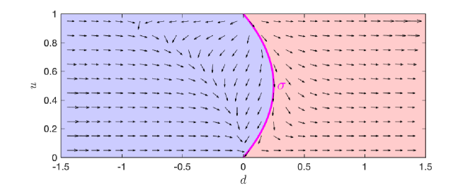
Figure 1. The flow map and the critical threshold in $(d,u)$-plane

3.1. The sharp critical threshold

We define the critical threshold that distinguishes the two regions in Figure 1 as $d=\sigma(u)$. The function $\sigma:[0,1]\to\mathbb{R}$ should satisfy the following ODE

$$\sigma^{\prime}(x)=\frac{2\sigma^{2}-(3x-5x^{2})\sigma-x^{3}(1-x)}{-x^{2}(1-x)},\quad\sigma(0)=0.$$ (24)

In particular, $\sigma^{\prime}(0)$ can be determined by

$$\sigma^{\prime}(0)= \lim_{x\to 0}\frac{2\sigma(x)^{2}-(3x-5x^{2})\sigma(x)-x^{3}(1-x)}{-x^{2}(1-x)}$$

$$= -2\left(\lim_{x\to 0}\frac{\sigma(x)}{x}\right)^{2}+3\lim_{x\to 0}\frac{\sigma(x)}{x}=-2\sigma^{\prime}(0)^{2}+3\sigma^{\prime}(0).$$

This implies $\sigma^{\prime}(0)=1$.

Therefore, (24) uniquely defines a function $\sigma$.

3.2. Global regularity for subcritical initial data

We now prove the first part of Theorem 1.1. The goal is to show that, if the initial data satisfy (10), then condition (12) holds for any time $T$. Equivalently, we will show $d=\partial_{x}u$ is bounded along all characterstic paths.

First, we show an upper bound of $d$.

Proposition 3.1 (Invariant region).

Let $(d,u)$ satisfy the dynamics (22) with initial condition $d_{0}\leq\sigma(u_{0})$. Then, $d(t)\leq\sigma(u(t))$ for any time $t\geq 0$.

Proof.

We first consider two special cases $u_{0}=0$ and $u_{0}=1$. In both cases, $\dot{u}=0$ and hence $u$ does not change in time.

For $u_{0}=0$, the dynamics of $d$ becomes

$$\dot{d}=2d^{2}e^{-\bar{u}}.$$ (25)

If $d_{0}\leq\sigma(0)=0$, clearly $d(t)\leq 0$ for any $t\geq 0$.

For $u_{0}=1$. the dynamics of $d$ becomes

$$\dot{d}=2d(d+1)e^{-\bar{u}}.$$ (26)

Again, if $d_{0}\leq\sigma(1)=0$, then $d(t)\leq 0$ for any $t\geq 0$.

Next, we consider the case $u_{0}\in(0,1)$. Here, we use the fact that trajectories do not cross. To be more precise, we argue by a contradiction. Suppose there exists a time $t$ such that $d(t)>\sigma(u(t))$. Then, there must exist a time $t_{0}$ so that the $(d,u)$ first exit the region at $t_{0}+$. By continuity, $d(t_{0})=\sigma(u(t_{0}))$. Starting from $(d(t_{0}),u(t_{0}))$, the trajectory satisfies (23).

By definition (24), $d=\sigma(u)$ is a solution in the phase plane. The standard Cauchy-Lipschitz theorem ensures that (23) with initial condition $(d(t_{0}),u(t_{0}))$ has a local unique solution. Therefore, the solution has to be $d(t_{0}+)=\sigma(u_{0}(t_{0}+))$. This contradicts the assumption that $(d,u)$ exit the region at $t_{0}+$. ∎

Next, we show a lower bound of $d$. This can be easily observed by Figure 1, as the flow is moving to the right as long as $d<-1$.

Proposition 3.2.

Let $(d,u)$ satisfy the dynamics (22). Then, for any $t\geq 0$,

$$d(t)\geq\min\{-1,d_{0}\}.$$

Proof.

We rewrite

$$\dot{d}=2(d-d_{-})(d-d_{+})e^{-\bar{u}},\quad d_{\pm}=\frac{(3u-5u^{2})\pm\sqrt{(3u-5u^{2})^{2}+8u^{3}(1-u)}}{4}.$$

Then, $\dot{d}\geq 0$ if $d\leq d_{-}$. This implies $d(t)\geq\min\{d_{-},d_{0}\}$. Note that for $u\in[0,1]$, $d_{-}\geq 1$. Therefore, we obtain the lower bound. ∎

Combining the two bounds, we know that along each characteristic path, $d$ is bounded in all time. Collecting all characterstic paths, we obtain $\|\partial_{x}u(t,\cdot)\|_{L^{\infty}}$ is bounded for any $t\geq 0$. Global regularity then follows from Theorem 2.1.

3.3. Finite time breakdown for supercritical initial data

We turn to prove the second part of Theorem 1.1. Suppose the initial data satisfy (11). Then, we consider the characteristic path originated at $x_{0}$, namely $d_{0}=u_{0}^{\prime}(x_{0})$ and $u_{0}=u_{0}(x_{0})$. So,

$$d_{0}>\sigma(u_{0}).$$ (27)

For $u_{0}=0$ or $u_{0}=1$, finite time blow up can be easily obtain by the Ricatti-type dynamics (25) and (26). Moreover, as $0\leq u\leq 1$, we must have $d_{0}=0$ when $u_{0}=0$ or $1$. Therefore, there is no supercritical data with $u_{0}=0$ or $1$.

We focus on the case when $u_{0}\in(0,1)$. The main idea is illustrated in Figure 2. For each trajectory starting at a supercritical initial point $(d_{0},u_{0})$, $u$ is getting close to 0 as time evolves, unless blowup already happens. When $u$ becomes close to 0, the dynamics of $d$ becomes close to (25). Then, if $d$ is away from 0, the Ricatti-type dynamics will lead to a finite time blowup.

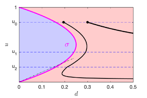
Figure 2. An illustration of typical trajectories with supercritical initial data $(d_{0},u_{0})$. Case 1: blow up happens before the trajectory reaches $u_{1}$. Case 2: the trajectory passes $u_{1}$, but blow up eventually happens in finite time.

To rigorously justify the idea, we first examine the dynamics of $u$ in (22).

Proposition 3.3.

Let $(d,u)$ be a solution of (22) with supercritical initial data $(d_{0},u_{0})$. Then, for any $u_{1}\in(0,u_{0})$, there exists a finite time $t_{1}$ such that, either $d(t)\to\infty$ before $t_{1}$, or $u(t_{1})\leq u_{1}$.

Proof.

Using the bound on the nonlocal term (16), we get

$$\dot{u}\leq-e^{-m}u^{2}(1-u).$$

As long as $(d,u)$ is bounded, the characterstic path stays valid.

The following comparison principle holds. Let $\eta=\eta(t)$ satisfy the ODE

$$\eta^{\prime}=-e^{-m}\eta^{2}(1-\eta),\quad\eta(0)=u_{0}.$$ (28)

Then, $u(t)\leq\eta(t)$. Indeed,

$$\dot{u}(t)-\eta^{\prime}(t)\leq e^{-m}\left(-u^{2}(1-u)+\eta^{2}(1-\eta)\right)\leq 3e^{-m}(u-\eta).$$

This implies

$$u(t)-\eta(t)\leq(u(0)-\eta(0))e^{3e^{-m}t}\leq 0.$$

The dynamics $\eta$ in (28) can be solved explicitly

$$\left.\left(\frac{1}{\eta}+\log\frac{1-\eta}{\eta}\right)\right]_{u_{0}}^{\eta(t)}=e^{-m}t.$$

Therefore, $\eta(t_{1})=u_{1}$ at

$$t_{1}=e^{m}\left(\frac{1}{u_{1}}+\log\frac{1-u_{1}}{u_{1}}-\frac{1}{u_{0}}-\log\frac{1-u_{0}}{u_{0}}\right)<+\infty.$$

Applying the comparison principle, we end up with $u(t_{1})\leq u_{1}$. ∎

Proposition 3.3 distinguishes the two cases illustrated in Figure 2. Either blowup happens before $u$ reaches $u_{1}$, which takes finite time, or the trajectory passes $u_{1}$. We shall focus on the latter case from now on.

Next, we argue that by picking a small enough $u_{1}>0$, the dynamics (22) will lead to a blowup in finite time, as long as $d$ stays away from zero.

Proposition 3.4.

Let $(d,u)$ be a solution of (22). Suppose $d$ is uniformly bounded away from zero, namely there exists a $C_{*}>0$ such that

$$d(t)\geq C_{*},\quad\forall~{}t\geq 0.$$ (29)

Then, there exists a $u_{1}>0$, depending on $C_{*}$, such that, with the initial condition $(d(t_{1}),u(t_{1})=u_{1})$, the solution has to blow up in finite time.

Proof.

As $u(t_{1})=u_{1}$, we know $u(t)\leq u_{1}$ for any $t\geq t_{1}$. Then, we get

$$\dot{d}\geq e^{-\bar{u}}(2d^{2}-3u_{1}d-u_{1}^{3})=2e^{-\bar{u}}(d-d_{-})(d-d_{+}),\quad d_{\pm}=\frac{3\pm\sqrt{9+8u_{1}}}{4}u_{1}.$$

Pick $u_{1}=C_{*}/4$, then

$$d(t_{1})\geq C_{*}=4u_{1}>2d_{+}.$$

This implies $d(t)>2d_{+}$ for all $t\geq t_{1}$. We can then use (16) to bound the nonlocal term and get

$$\dot{d}\geq 2e^{-m}(d-d_{-})(d-d_{+}),\quad\forall~{}t\geq t_{1}.$$ (30)

Then, by a comparison principle (similar as the one used in Proposition 3.3), the solution

$$d(t)\geq\frac{d_{-}e^{2e^{-m}(d_{+}-d_{-})(t-t_{1})}(d(t_{2})-d_{+})-d_{+}(d(t_{1})-d_{-})}{e^{2e^{-m}(d_{+}-d_{-})(t-t_{1})}(d(t_{1})-d_{+})-(d(t_{1})-d_{-})},$$

where the right hand side is the exact solution of the ODE (30) with an equal sign. It blows up at

$$T_{*}=t_{1}+\frac{1}{2e^{-m}(d_{+}-d_{-})}\log\frac{d(t_{1})-d_{-}}{d(t_{1})-d_{+}}<t_{1}+\frac{2e^{m}}{C_{*}}<+\infty.$$

Therefore, $d$ has to blow up no later than $T_{*}$. ∎

We are left to show the uniform lower bound on $d$, i.e. condition (29), for any supercritical initial data. We shall work with trajectories in the phase plane.

Let us denote $d=d(u)$ be the trajectory that go through $(d_{0},u_{0})$. As both $d$ and $\sigma$ satisfy (23), we compute

$$(d(u)-\sigma(u))^{\prime}=\frac{2(d(u)+\sigma(u))-(3u-5u^{2})}{-u^{2}(1-u)}(d(u)-\sigma(u))=:A(u)(d(u)-\sigma(u)).$$

Since $(d_{0},u_{0})$ satisfy (27), we get $d(u_{0})-\sigma(u_{0})>0$. $A(u)$ is bounded as long as $u$ stays away from 0 and 1. Therefore, we obtain

$$d(u)\geq\sigma(u)\geq 0,\quad\forall~{}u\in(0,1).$$

Moreover, for any $u\in(0,u_{0})$, we can estimate $A$ by

$$A(u)\leq\frac{3-5u}{u(1-u)}\leq\frac{3}{u}.$$

Integrating in $[u,u_{0}]$, we get

$$d(u)\geq d(u)-\sigma(u)=(d_{0}-\sigma(u_{0}))\exp\left[-\int_{u}^{u_{0}}A(u)du\right]\geq\frac{(d_{0}-\sigma(u_{0}))}{u_{0}^{3}}u^{3}.$$ (31)

Unfortunately, this bound is not uniform in $(0,u_{0}]$. We need an enhanced estimate.

Let $u_{2}>0$ such that

$$\sigma(u)\geq\frac{3}{4}u,\quad\forall~{}u\in[0,u_{2}].$$ (32)

Note that such $u_{2}$ exists as $\sigma^{\prime}(0)=1$.

For $u\in(0,u_{2}]$, using (32), we obtain an improved estimate on $A$ as follows.

$$A(u)\leq\frac{4\sigma(u)-(3u-5u^{2})}{-u^{2}(1-u)}\leq\frac{3u-(3u-5u^{2})}{-u^{2}(1-u)}=\frac{-5}{1-u}\leq-5.$$

Since $A(u)$ is negative, we immediately get

$$d(u)\geq d(u)-\sigma(u)\geq d(u_{2})-\sigma(u_{2}),\quad\forall~{}u<u_{2},~{}u\in\textnormal{Dom}(d).$$

This, together with (31), shows a uniformly lower bound on $d$

$$d(u)\geq\frac{d_{0}-\sigma(u_{0})}{u_{0}^{3}}u_{2}^{3},\quad\forall~{}u\leq u_{0},~{}u\in\textnormal{Dom}(d).$$

Condition (29) follows immediately, with $C_{*}=(d_{0}-\sigma(u_{0}))u_{2}^{3}u_{0}^{-3}$.

4. Examples and simulations

In this section, we present examples and numerical simulations to illustrate our main critical threshold result, Theorem 1.1.

The numerical method we use is the standard finite volume scheme, with a large enough computational domain. One can consult [16] for an extensive discussion on the numerical implementation.

We shall also compare the numerical results for the three different types of nonlocal interaction kernels. Recall

$$K(x)=\begin{cases}0,&\text{{\color[rgb]{0,0,1}\char 172} LWR model: look-ahead distance }L=0,\\ 1_{[-1,0)}(x),&\text{{\color[rgb]{1,0,1}\char 173} SK model: look-ahead distance }L=1,\\ 1_{(-\infty,0]}(x),&\text{{\color[rgb]{1,0,0}\char 174} Our model: look-ahead distance }L=\infty,\\ 1,&\text{\char 175 LWR model: globally uniform kernel},\\ \end{cases}$$ (33)

Here, $1_{A}$ denotes the indicator function of a set $A$.

4.1. Supercritical initial data

Many smooth initial data $u_{0}$ lie in the supercritical region (11). In particular, we argue that all compactly supported smooth function lies in the supercritical region.

Proposition 4.1.

Let $u_{0}\in C^{1}(\mathbb{R})$ is non-negative and compactly supported. Then, $u_{0}$ satisfies the supercritical condition (11).

Proof.

We argue by contradiction. Suppose $u_{0}$ lies in the subcritical region. Then, we have

$$u_{0}^{\prime}(x)\leq u_{0}(x),\quad\forall~{}x\in\mathbb{R}.$$ (34)

Let $x_{L}$ be the left end point of the support of $u_{0}$, namely

$$x_{L}=\arg\inf_{x}\{u_{0}(x)>0\}.$$

By continuity, we know $u_{0}(x_{L})=0$. Solving the ODE (34) with initial condition at $x_{L}$ yields

$$u_{0}(x)\leq 0,\quad\forall~{}x\geq x_{L}.$$

This contradicts with the definition of $x_{L}$. Hence, $u_{0}$ can not lie in the subcritical region. It must be supercritical. ∎

As an example, let us take the following smooth and compactly supported initial data.

$$u_{0}(x)=\begin{cases}e^{-\frac{1}{1-x^{2}}},&|x|<1,\\ 0,&|x|\geq 1.\end{cases}$$ (35)

Figure 3 shows the contour plot of $(u_{0}^{\prime}(x),u_{0}(x))$ in the phase plane for all $x\in\mathbb{R}$. Clearly, the curve does not lie in the subcritical region. So, $u_{0}$ is supercritical. Theorem 1.1 then implies a finite time wave break-down.

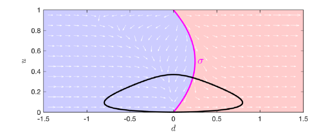
Figure 3. The contour plot of $(u^{\prime}_{0}(x),u_{0}(x))$ in the phase plane where $u_{0}$ is (35). This initial condition lies in the supercritical region.

Figure 4 shows the numerical result for the model with initial data (35), together with other models. The wave break-down can be easily observed, which matches our theoretical result.

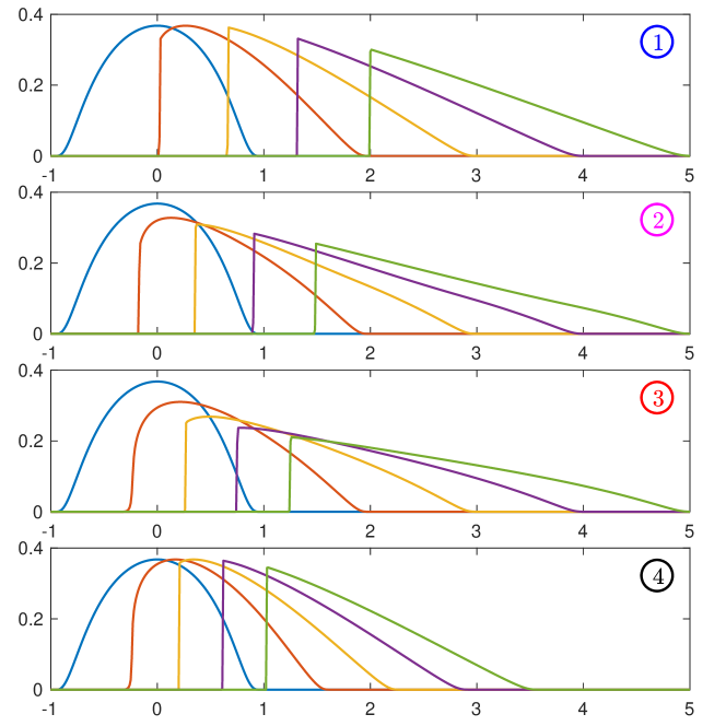
Figure 4. Snapshots of solutions for the dynamics for the four kernels, with supercritical initial condition (35) at time $t=0,1,2,3,4$.

Note that since

$$0\leq 1_{[-1.0)}(x)\leq 1_{(-\infty,0]}(x)\leq 1,\quad\forall~{}x\in\mathbb{R},$$ (36)

model ① has the fastest wave speed, while model ④ has the slowest. This is indeed captured in the numerical result.

4.2. Subcritical initial data

We now construct an initial condition $u_{0}$ that lies in the subcritical region (10).

Due to Proposition 4.1, $u_{0}$ can not be compactly supported. Moreover, we need $u_{0}\in L^{1}(\mathbb{R})$. One valid choice is that $u_{0}$ decays algebraically when $x\to-\infty$, namely $u_{0}(x)\sim(-x)^{-\beta}$ for $\beta>1$. We can check

$$\lim_{x\to-\infty}\frac{u_{0}^{\prime}(x)}{u_{0}(x)}=\lim_{x\to-\infty}\frac{\beta(-x)^{-\beta-1}}{(-x)^{-\beta}}=0<1.$$

Therefore, $(u_{0}^{\prime}(x),u_{0}(x))$ should lie in the subcritical region of the phase plane when $x$ is very negative.

For large $x$, the choice of $u_{0}$ is less critical. As long as $u_{0}^{\prime}(x)\leq 0$, it always lies in the subcritical region. We can either choose $u_{0}$ vanishes for large $x$, or it decays fast as $x\to+\infty$.

Here is a subcritical initial condition

$$u_{0}(x)=\begin{cases}1/x^{2},&x\in(-\infty,-3],\\ (3x^{5}+35x^{4}+123x^{3}+81x^{2}-162x+162)/1458,&x\in(-3,0],\\ e^{-x}/9,&x\in(0,\infty).\end{cases}$$ (37)

The middle part is chosen as a polynomial which smoothly connects the two functions, so that $u\in C^{2}(\mathbb{R})$.

The contour plot of $(u_{0}^{\prime}(x),u_{0}(x))$ is shown in Figure 5, which indicates $u_{0}$ is subcritical. Therefore, as a consequence of Theorem 1.1, the solution should be globally regular.

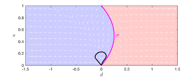
Figure 5. The contour plot of $(u^{\prime}_{0}(x),u_{0}(x))$ in the phase plane where $u_{0}$ is (37). This initial condition lies in the subcritical region.

Figure 6 shows the numerical results for all four models with initial conditon (37). We observe that the solution of our model ③ indeed does not generate shocks.

The wave speeds of the four models behave similar as the supercritical case, due to (36). However, very interestingly, our model ③ is the only model where there is no finite time wave break-down. Indeed, we plot the quantity $\|\partial_{x}u(\cdot,t)\|_{L^{\infty}}/\|u(\cdot,t)\|_{L^{\infty}}$ against time $t$ in Figure 7. The quantity blows up in finite time for models ①, ② and ④, but remains bounded for our model ③.

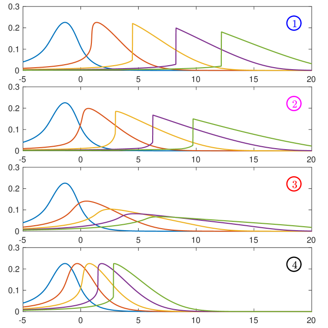
Figure 6. Snapshots of solutions for the dynamics for the four kernels, with subcritical initial condition (37) at time $t=0,5,10,15,20$.

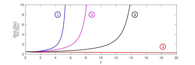
Figure 7. Numerical indicators of finite time blowup versus global regularity. With initial condition (37), only our kernel ③ has a global smooth solution.

5. Further discussion

We have shown a sharp critical threshold for our traffic model (1) with look-ahead kernel (9). We also compare our model with other classical kernels (33) through numerical simulations. Our kernel has a unique feature that the solution remains globally regular for initial conditions like (37).

To understand such behavior, we shall focus on the nonlocal slow down factor $e^{-\bar{u}}$. From (36), we observe that our model has a factor which is neither the largest nor the smallest. Hence, the size of the slow down factor does not matter.

An important feature of our model is that, the slow down factor is monotone increasing. Indeed, we have

$$\partial_{x}e^{-\bar{u}}=ue^{-\bar{u}}>0,\quad\forall~{}x\text{~{}~{}s.t.~{}~{}}u(x)>0.$$

This implies that the front crowd does not slow down as much as the back crowd. This could help avoid the shock formation, as observed in the example.

For general nonlocal look-ahead kernel, it remains open whether there are subcritical initial data which lead to global regularity. If we consider a family of kernel $K_{L}$ in (6), our result indicates that subcritical initial data exist for $L=\infty$. On the other hand, subcritical initial data does not exist for the LWR model, where $L=0$. For $L\in(0,\infty)$, the problem is open. A conjecture is, subcritical initial data exists for $L$ large enough. This will be left for future investigation.

Appendix A Composition estimate

In this section, we show the following estimate on the composition of two functions. The estimate is useful to control the nonlocal weight $e^{-\bar{u}}$ for our system.

Theorem A.1.

Let $s>0$. Suppose $g\in L^{\infty}\cap\dot{H}^{s}(\mathbb{R})$ and $f\in C^{\lceil s\rceil}(\textnormal{Range}(g))$. Then, the composition $f\circ g\in L^{\infty}\cap\dot{H}^{s}(\mathbb{R})$. Moreover, there exists a constant $C>0$, depending on $s,\|f\|_{C^{\lceil s\rceil}}$ and $\|g\|_{L^{\infty}}$, such that

$$\|f\circ g\|_{\dot{H}^{s}}\leq C\|g\|_{\dot{H}^{s}}.$$

Proof.

We first consider the case when $s$ is an integrer. Express $\partial_{x}^{s}(f(g(x)))$ using Faà di Bruno’s formula

$$\partial_{x}^{s}(f(g(x)))=\sum_{\alpha\in S_{s}}C_{\alpha}(x)\prod_{r=1}^{s}(\partial_{x}^{r}g(x))^{\alpha_{r}}.$$

where

$$S_{s}=\left\{\alpha=(\alpha_{1},\cdots,\alpha_{s})~{}:~{}a_{k}\in\mathbb{N},~{}~{}\sum_{r=1}^{s}r\alpha_{r}=s,~{}~{}\sum_{r=1}^{s}\alpha_{r}\leq s.\right\}.$$

and

$$C_{\alpha}(x)=s!\prod_{r=1}^{s}\left(\frac{1}{\alpha_{r}!\cdot(r!)^{\alpha_{r}}}\right)\partial_{x}^{\nu(\alpha)}f(g(x)),\quad\nu(\alpha)=\sum_{r=1}^{s}\alpha_{r}.$$

Then,

$$\|\partial_{x}^{s}(f\circ g)\|_{L^{2}}\leq\sum_{\alpha\in S_{s}}\|C_{\alpha}\|_{L^{\infty}}\left\|\prod_{r=1}^{s}(\partial_{x}^{r}g)^{\alpha_{r}}\right\|_{L^{2}}\lesssim\|f\|_{C^{s}}\sum_{\alpha\in S_{s}}\left\|\prod_{r=1}^{s}(\partial_{x}^{r}g)^{\alpha_{r}}\right\|_{L^{2}}.$$

Now, we estimate the last term. Applying Hölder’s inequality, we get

$$\left\|\prod_{r=1}^{s}(\partial_{x}^{r}g)^{\alpha_{r}}\right\|_{L^{2}}\leq\prod_{r=1}^{s}\|(\partial_{x}^{r}g)^{\alpha_{r}}\|_{L^{p_{r}}}=\prod_{r=1}^{s}\|\partial_{x}^{r}g\|_{L^{\alpha_{r}p_{r}}}^{\alpha_{r}},$$

where $\{p_{r}\}_{r=1}^{s}$ is chosen as $p_{r}=\frac{2s}{r\alpha_{r}}$. So we have

$$\sum_{r=1}^{s}\frac{1}{p_{r}}=\frac{1}{2s}\sum_{r=1}^{s}r\alpha_{r}=\frac{1}{2}.$$

For each term $\|\partial_{x}^{r}g\|_{L^{\alpha_{r}p_{r}}}$, we apply Gagliardo-Nirenberg-Sobolev interpolation inequality

$$\|\partial_{x}^{r}g\|_{L^{\alpha_{r}p_{r}}}=\|\partial_{x}^{r}g\|_{L^{\frac{2s}{r}}}\lesssim\|\partial_{x}^{s}g\|_{L^{2}}^{\frac{r}{s}}\|g\|_{L^{\infty}}^{1-\frac{r}{s}}.$$

Collecting all terms together, we obtain

$$\prod_{r=1}^{s}\|\partial_{x}^{r}g\|_{L^{\alpha_{r}p_{r}}}^{\alpha_{r}}\lesssim\|\partial_{x}^{s}g\|_{L^{2}}^{\sum_{r=1}^{s}\alpha_{r}\frac{r}{s}}\|g\|_{L^{\infty}}^{\sum_{r=1}^{s}\alpha_{r}(1-\frac{r}{s})}=\|\partial_{x}^{s}g\|_{L^{2}}\|g\|_{L^{\infty}}^{\nu(\alpha)-1}.$$

This concludes the proof.

Next, we discuss the case when $s$ is not an integer. For $s\in(0,1)$, one can directly apply the chain rule for fractional derivatives [8, Proposition 3.1]

$$\|f\circ g\|_{\dot{H}^{s}}\leq C\|\partial_{x}f\|_{L^{\infty}}\|g\|_{\dot{H}^{s}}.$$

where $C$ is a constant depending on $s$ and $\|g\|_{L^{\infty}}$.

For $s>1$, we can combine the estimate for $\lfloor s\rfloor$ and the fractional chain rule for $s-\lfloor s\rfloor$. The detail will be left to the readers. ∎

References

- [1] Hajer Bahouri, Jean-Yves Chemin, and Raphaël Danchin. Fourier analysis and nonlinear partial differential equations, volume 343. Springer Science & Business Media, 2011.
- [2] Andrea L Bertozzi, José A Carrillo, and Thomas Laurent. Blow-up in multidimensional aggregation equations with mildly singular interaction kernels. Nonlinearity, 22(3):683, 2009.
- [3] Andrea L Bertozzi, Thomas Laurent, and Jesús Rosado. theory for the multidimensional aggregation equation. Communications on Pure and Applied Mathematics, 64(1):45–83, 2011.
- [4] Fernando Betancourt, Raimund Bürger, Kenneth H Karlsen, and Elmer M Tory. On nonlocal conservation laws modelling sedimentation. Nonlinearity, 24(3):855, 2011.
- [5] Martin Burger, Yasmin Dolak-Struss, Christian Schmeiser, et al. Asymptotic analysis of an advection-dominated chemotaxis model in multiple spatial dimensions. Communications in Mathematical Sciences, 6(1):1–28, 2008.
- [6] José A Carrillo, Young-Pil Choi, Eitan Tadmor, and Changhui Tan. Critical thresholds in 1D Euler equations with nonlocal forces. Mathematical Models and Methods in Applied Sciences, 26(1):185–206, 2016.
- [7] José A Carrillo, Marco DiFrancesco, Alessio Figalli, Thomas Laurent, and Dejan Slepčev. Global-in-time weak measure solutions and finite-time aggregation for nonlocal interaction equations. Duke Mathematical Journal, 156(2):229–271, 2011.
- [8] FM Christ and Michael I Weinstein. Dispersion of small amplitude solutions of the generalized Korteweg-de Vries equation. Journal of functional analysis, 100(1):87–109, 1991.
- [9] Adrian Constantin and Joachim Escher. Wave breaking for nonlinear nonlocal shallow water equations. Acta Mathematica, 181(2):229–243, 1998.
- [10] Yasmin Dolak and Christian Schmeiser. The Keller–Segel model with logistic sensitivity function and small diffusivity. SIAM Journal on Applied Mathematics, 66(1):286–308, 2005.
- [11] Shlomo Engelberg, Hailiang Liu, and Eitan Tadmor. Critical thresholds in Euler-Poisson equations. Indiana University Mathematics Journal, 50:109–157, 2001.
- [12] Darryl D Holm and NW Hone. A class of equations with peakon and pulson solutions (with an appendix by Harry Braden and John Byatt-Smith). Journal of Nonlinear Mathematical Physics, 12(sup1):380–394, 2005.
- [13] John K Hunter. Numerical solutions of some nonlinear dispersive wave equations. Lect. Appl. Math, 26:301–316, 1990.
- [14] Vera Mikyoung Hur. Wave breaking in the Whitham equation. Advances in Mathematics, 317:410–437, 2017.
- [15] Tosio Kato and Gustavo Ponce. Commutator estimates and the Euler and Navier-Stokes equations. Communications on Pure and Applied Mathematics, 41(7):891–907, 1988.
- [16] Alexander Kurganov and Anthony Polizzi. Non-oscillatory central schemes for traffic flow models with Arrhenius look-ahead dynamics. NHM, 4(3):431–451, 2009.
- [17] George J Kynch. A theory of sedimentation. Transactions of the Faraday society, 48:166–176, 1952.
- [18] Yongki Lee. Wave breaking in a class of non-local conservation laws. arXiv preprint arXiv:1812.10406, 2018.
- [19] Yongki Lee and Hailiang Liu. Thresholds in three-dimensional restricted euler–poisson equations. Physica D: Nonlinear Phenomena, 262:59–70, 2013.
- [20] Yongki Lee and Hailiang Liu. Threshold for shock formation in the hyperbolic Keller–Segel model. Applied Mathematics Letters, 50:56–63, 2015.
- [21] Yongki Lee and Hailiang Liu. Thresholds for shock formation in traffic flow models with Arrhenius look-ahead dynamics. Discrete & Continuous Dynamical Systems-A, 35(1):323–339, 2015.
- [22] Dong Li. On Kato-Ponce and fractional leibniz. Revista Matematica Iberoamericana, 35(1):23–100, 2019.
- [23] Hailiang Liu. Wave breaking in a class of nonlocal dispersive wave equations. Journal of Nonlinear Mathematical Physics, 13(3):441–466, 2006.
- [24] Alexandros Sopasakis and Markos A Katsoulakis. Stochastic modeling and simulation of traffic flow: asymmetric single exclusion process with Arrhenius look-ahead dynamics. SIAM Journal on Applied Mathematics, 66(3):921–944, 2006.
- [25] Eitan Tadmor and Hailiang Liu. Critical thresholds in 2D restricted Euler-Poisson equations. SIAM Journal on Applied Mathematics, 63(6):1889–1910, 2003.
- [26] Eitan Tadmor and Changhui Tan. Critical thresholds in flocking hydrodynamics with non-local alignment. Philosophical Transactions of the Royal Society A: Mathematical, Physical and Engineering Sciences, 372(2028):20130401, 2014.
- [27] Changhui Tan. Singularity formation for a fluid mechanics model with nonlocal velocity. arXiv preprint arXiv:1708.09360, 2017.
- [28] Changhui Tan. On the Euler-Alignment system with weakly singular communication weights. arXiv preprint arXiv:1901.02582, 2019.
- [29] VO Vakhnenko and EJ Parkes. The calculation of multi-soliton solutions of the Vakhnenko equation by the inverse scattering method. Chaos, Solitons & Fractals, 13(9):1819–1826, 2002.
- [30] Gerald Beresford Whitham. Linear and nonlinear waves, volume 42. John Wiley & Sons, 2011.
- [31] Kevin Zumbrun. On a nonlocal dispersive equation modeling particle suspensions. Quarterly of Applied Mathematics, 57(3):573–600, 1999.