Pion and Kaon form factors in the perturbative QCD approach

Abstract

We present the most accurate calculation for the pion and kaon electromagnetic form factors in the framework of perturbative QCD, where the power corrections up to twist-4 of the meson distribution amplitudes and the next-to-leading-order QCD corrections up to subleading power are included. In order to guarantee the gauge invariance of the meson to vacuum matrix element, we take into account both assignments with the lowest Fock state and the high Fock state with an additional valence gluon. Our results confirm the power behaviour of the twist expansion and show the chiral enhancement effect at subleading power in the PQCD approach. We also estimate the $\mathrm{SU(3)}$ asymmetry for the kaon and pion form factors and find that it is smaller than $30\%$.

I Introduction

The Quantum chromodynamics (QCD) has two fundamental properties: the quark confinement in the low energy region and the asymptotic freedom in the high energy region. The confinement leads to the formation of the hadrons, while the asymptotic freedom of the strong interaction results in the perturbative QCD calculations. When an energetic photon hit a constituent parton (quark, antiquark or gluon, etc ) inside a hadron, one uses a function ” form factor” to describe the redistribution of the momenta of the parton inside the hadron. The form factor therefore carries both the information of hadron structure and the hard scattering amplitude. In order to calculate the form factor for a given transition process, the factorization theory is developed to help one to separate the pertubative and nonperturbative contributions LepageZA ; LepageFJ ; EfremovQK . The electromagnetic (e.m.) form factor of pion, being the simplest but simultaneously the most fundamental QCD observed quantity, attracts much attention both in theory GoussetYH ; ff-pion-QCDSRs ; ff-pion-LCSRs ; ff-pion-PQCD ; ff-pion-LQCD and in experiments prd9-1229 ; prl95-261803 ; prl97-192001 .

The statements for the form factors are rather different in different theoretical approaches. In the QCD factorization (QCDF) BenekeBR ; BauerEW ; Beneke:2002ph , for example, the form factor is the nonpertuabtive input. In the light-cone sum rules (LCSRs), one believes that the soft dynamics will provide the dominate contribution ff-pion-LCSRs . In the perturbative QCD (PQCD) approach, however, it is described by a hard scattering amplitude LiUN ; ff-pion-PQCD and can be calculated perturbatively. For the pion form factor, for instance, the lattice QCD (LQCD) evaluation is still available at a few points of the momentum transfer squared $Q^{2}$ so far ff-pion-LQCD , while the direct experiment measurements are credible below $3$ GeV² prl95-261803 ; prl97-192001 too. The LCSRs approach is reliable in the intermediate region $1\leq Q^{2}\leq 15$ GeV² BelyaevZK , and the prediction power of the PQCD approach holds well in the large region $Q^{2}\geq 10\,\mathrm{GeV}^{2}$ with the inclusion of the resummation effects. In this paper we calculate the higher power corrections to pion and kaon form factors up to twist-4 of the meson DAs, with the aim to check the power expansion behaviour from one side, and from the other side to improve the theoretical accuracy in the framework of PQCD approach.

The rest of the paper is organized as follows. In Sec.II, the PQCD calculation of the spacelike pion form factor is performed by considering both the quark-antiquark and the quark-antiquark-gluon assignments. In Sec.III, we present the procedure of the PQCD approach to calculate the pion form factor, several important issues are highlighted. Sec.IV contains the numerical results and we conclude in Sec.V.

II Power corrections

The pion form factor is defined by the nonlocal matrix element

$$\langle\pi^{-}(p_{2})|J_{\mu}^{\mathrm{e.m.}}|\pi^{-}(p_{1})\rangle\equiv e_{q}(p_{1}+p_{2})F_{\pi}(Q^{2})\,,$$ (1)

we are interest in the case that the smallness of relative distance is ensured by the ”external reason”, says large momentum transfer between the hadrons, in this case $\overline{z}_{i}\overline{p}_{i}\sim 1$ and the expansion parameter for a given operator is the twist (dimension minus spinor). To separate the amplitude of matrix element contributed from the short- and long-distance interactions, we replace the lines with large virtuality by the free propagators, while retain the lines with small virtuality in the Heisenberg operator. In this way the matrix element can be written in the factorizable form,

$$\langle\pi^{-}(p_{2})|J_{\mu}^{\mathrm{e.m.}}|\pi^{-}(p_{1})\rangle= \oint dz_{1}dz_{2}\,\big{\langle}\pi^{-}(p_{2})\bigg{|}\left\{\overline{d}_{\gamma}(0)\,\mathrm{exp}\left(ig_{s}\int_{z_{2}}^{0}d\sigma_{\nu^{\prime}}A_{\nu^{\prime}}(\sigma)\right)u_{\beta}(z_{2})\right\}_{kj}\bigg{|}0\big{\rangle}_{\mu_{t}}$$ (2)

$$\,\cdot\,H_{\gamma\beta\alpha\delta}^{ijkl}(z_{1},z_{2})\,\cdot\,\big{\langle}0\bigg{|}\left\{\overline{u}_{\alpha}(z_{2})\,\mathrm{exp}\left(ig_{s}\int_{z_{1}}^{z_{2}}d\sigma_{\nu}A_{\nu}(\sigma)\right)d_{\delta}(z_{1})\right\}_{il}\bigg{|}\pi^{-}(p_{1})\big{\rangle}_{\mu_{t}}\,,$$

where $\gamma,\beta,\alpha,\delta$ are the spinor indices, and $i,j,k,l$ are the color indicators. In Eq. (2), the hard kernel associated with the lowest Fock state is

$$H_{\gamma\beta\alpha\delta}^{ijkl}(z_{1},z_{2})=(-1)\left[ig_{s}\gamma_{m}\right]_{\alpha\beta}T^{ij}\left[(ie_{q}\gamma_{\mu})S_{0}(0-z_{1})(ig_{s}\gamma_{n})\right]_{\gamma\delta}T^{kl}\left[-iD_{mn}^{0}(z_{1}-z_{2})\right]\,,$$ (3)

where the factor $(-1)$ comes from the anti-communicativity of the quark operator, and the free propagators are written in the coordinate space as

$$S_{0}(z)=\frac{i}{2\pi}\frac{z/}{z^{4}}\,,\,\,\,\,\,\,D_{mn}^{0}(z)=\frac{1}{4\pi}\frac{g_{mn}}{z^{2}}\,.$$ (4)

The nonlocal matrix elements in Eq. (2) imply the amplitudes of mesons breaking-up into a pair of soft quarks, they receive contributions from different spin structures

$$\big{\langle}0\bigg{|}\left\{\overline{u}_{\alpha}(z_{2})\,\mathrm{exp}\left(ig_{s}\int_{z_{1}}^{z_{2}}d\sigma_{\nu}A_{\nu}(\sigma)\right)d_{\delta}(z_{1})\right\}_{il}\bigg{|}\pi^{-}(p_{1})\big{\rangle}_{\mu_{t}}$$

$$= \frac{\delta_{il}}{3}\left\{\frac{1}{4}\left(\gamma_{5}\gamma^{\rho}\right)_{\delta\alpha}\big{\langle}0\big{|}\overline{u}(z_{2})\,\mathrm{exp}\left(ig_{s}\int_{z_{1}}^{z_{2}}\,d\sigma_{\nu}A_{\nu}(\sigma)\right)\left(\gamma_{\rho}\gamma_{5}\right)d(z_{1})\big{|}\pi^{-}(p_{1})\big{\rangle}_{\mu_{t}}\right.$$ (5)

$$\left.\hskip 14.22636pt+\frac{1}{4}\left(i\gamma_{5}\right)_{\delta\alpha}\big{\langle}0\big{|}\overline{u}(z_{2})\,\mathrm{exp}\left(ig_{s}\int_{z_{1}}^{z_{2}}\,d\sigma_{\nu}A_{\nu}(\sigma)\right)\left(i\gamma_{5}\right)d(z_{1})\big{|}\pi^{-}(p_{1})\big{\rangle}_{\mu_{t}}\right.$$

$$\left.\hskip 14.22636pt+\frac{1}{8}\left(\sigma^{\tau\tau^{\prime}}\gamma_{5}\right)_{\delta\alpha}\big{\langle}0\big{|}\overline{u}(z_{2})\,\mathrm{exp}\left(ig_{s}\int_{z_{1}}^{z_{2}}\,d\sigma_{\nu}A_{\nu}(\sigma)\right)\left(i\sigma_{\tau\tau^{\prime}}\gamma_{5}\right)d(z_{1})\big{|}\pi^{-}(p_{1})\big{\rangle}_{\mu_{t}}\right.$$

$$\left.\hskip 14.22636pt+\cdots\right\}\,.$$

In the above expression, the ellipsis indicate the rest terms in the Fierz transformation, and the truncated scale of the integral $\mu_{t}$ is usually known as the factorizable scale. We quote the definition of Light-cone distribution amplitudes (LCDAs) of light pseudoscalar meson in appendix.A.

Substituting Eqs. (3,5 ) into Eq. (2) and taking into account the definition in Eq. (1), we obtain the pion e.m. form factor at each power with the two-parton-to-two-parton scattering,

$$F_{\pi}^{t2}(Q^{2}) = \frac{8}{9}\alpha_{s}\pi f_{\pi}^{2}Q^{2}\,\int\,\frac{d^{2}\mathbf{k}_{1T}}{(2\pi)^{2}}\,\frac{d^{2}\mathbf{k^{\prime}}_{1T}}{(2\pi)^{2}}\int_{0}^{1}dx\int_{0}^{1}dy\,\varphi_{\pi}(x)\varphi_{\pi}(y)\frac{\bar{y}}{\Delta_{1}^{2}\Delta_{2}^{2}}\,,$$ (6)

$$F_{\pi}^{t3,2p}(Q^{2}) = \frac{16}{9}\alpha_{s}\pi f_{\pi}^{2}m_{0}^{2}\,\int\,\frac{d^{2}\mathbf{k}_{1T}}{(2\pi)^{2}}\,\frac{d^{2}\mathbf{k^{\prime}}_{1T}}{(2\pi)^{2}}\int_{0}^{1}dx\int_{0}^{1}dy\,\frac{1}{\Delta_{1}^{2}\Delta_{2}^{2}}$$ (7)

$$\cdot\left[-y\,\varphi_{\pi}^{P}(x)\varphi_{\pi}^{P}(y)-\frac{1}{6}\varphi_{\pi}^{P}(x)\varphi_{\pi}^{\sigma}(y)\left(\frac{yQ^{2}}{\Delta_{1}^{2}}+\frac{(\bar{x}-\bar{y})Q^{2}}{\Delta_{2}^{2}}+1+\frac{(2-x)\bar{y}Q^{2}}{\Delta_{2}^{2}}\right)\right]\,,$$

$$F_{\pi}^{t2\otimes t4,2p}(Q^{2}) = \frac{16}{9}\alpha_{s}\pi f_{\pi}^{2}\,\int\,\frac{d^{2}\mathbf{k}_{1T}}{(2\pi)^{2}}\,\frac{d^{2}\mathbf{k^{\prime}}_{1T}}{(2\pi)^{2}}\int_{0}^{1}dx\int_{0}^{1}dy\,\Big{\{}\frac{\bar{x}\bar{y}Q^{2}}{\Delta_{1}^{2}\Delta_{2}^{4}}g_{2\pi}(x)\varphi_{\pi}(y)$$ (8)

$$+2\bar{y}Q^{2}\left[\frac{1}{\Delta_{1}^{2}\Delta_{2}^{4}}+\frac{\bar{y}(2-x)Q^{2}}{\Delta_{1}^{4}\Delta_{2}^{4}}+\frac{1}{\Delta_{1}^{4}\Delta_{2}^{2}}\right]\left[\varphi_{\pi}(x)g_{1\pi}(y)-\varphi_{\pi}(x)g^{{\dagger}}_{2\pi}(y)\right]$$

$$+\left[\frac{\bar{y}^{2}Q^{2}}{\Delta_{1}^{2}\Delta_{2}^{4}}+\frac{\bar{y}^{2}Q^{2}}{\Delta_{1}^{4}\Delta_{2}^{2}}\right]\varphi_{\pi}(x)g_{2\pi}(y)\,\Big{\}}\,.$$

The symbols of triangle in the above expressions represent the momentum carried by internal propagator: $\Delta_{1}=\bar{y}p_{2}-p_{1}=(-Q/\sqrt{2},\bar{y}Q/\sqrt{2},\mathbf{k}^{\prime})$, $\Delta_{2}=\bar{x}p_{1}-\bar{y}p_{2}=(\bar{x}Q/\sqrt{2},-\bar{y}Q/\sqrt{2},\mathbf{k}-\mathbf{k}^{\prime})$($\bar{y}=1-y$ and $\bar{x}=1-x$), in which $p_{1}$ and $p_{2}$ are the momentum of initial and final pions, respectively, $x$ and $y$ denote the momentum fraction carried by the quark in hadrons. The twist-2 times twist-4 contribution to the form factor is studied as the first time in the PQCD approach. To obtain Eq. (8), we have defined an auxiliary DA $g^{{\dagger}}_{2}(x)\equiv\int_{0}^{x}dx^{\prime}\,g_{2}(x^{\prime})$ with the bound condition $g^{{\dagger}}_{2}(x=0,1)=0$, and used the following Fourier transformations,

$$\frac{1}{x^{2}}\Leftrightarrow-i4\pi^{2}\frac{1}{p^{2}}\,,\,\,\,\,\,\,\frac{x_{\alpha}}{x^{2}}\Leftrightarrow 8\pi^{2}\frac{p_{\alpha}}{(p^{2})^{2}}\,,\,\,\,\,\,\,\frac{x_{\alpha}}{(x^{2})^{2}}\Leftrightarrow 2\pi^{2}\frac{p_{\alpha}}{p^{2}}\,,\,\,\,\,\,\,$$

$$\frac{x_{\alpha}x_{\beta}}{x^{2}}\Leftrightarrow\frac{-i8\pi^{2}}{(p^{2})^{2}}\left(g_{\alpha\beta}-4\frac{p_{\alpha}p_{\beta}}{p^{2}}\right)\,,\,\,\,\,\,\,\frac{x_{\alpha}x_{\beta}}{(x^{2})^{2}}\Leftrightarrow\frac{-i2\pi^{2}}{p^{2}}\left(g_{\alpha\beta}-2\frac{p_{\alpha}p_{\beta}}{p^{2}}\right)\,.$$ (9)

The Sudakov exponential from $k_{T}$ resummation, which would be discussed in the next section, suppresses the distribution of meson with wide transversal distance. We can omit the transversal momenta terms on the numerator in the large momentum transferred processes, then the second term on the right hand side of Eq. (8) vanishes, and the contributions associated with twist-3 DAs and twist-2 times twist-4 DAs reduce to

$$F_{\pi}^{t3,2p}(Q^{2}) \rightarrow \frac{16}{9}\alpha_{s}\pi f_{\pi}^{2}m_{0}^{2}\,\int\,\frac{d^{2}\mathbf{k}_{1T}}{(2\pi)^{2}}\,\frac{d^{2}\mathbf{k^{\prime}}_{1T}}{(2\pi)^{2}}\int_{0}^{1}dx\int_{0}^{1}dy\,\frac{1}{\Delta_{1}^{2}\Delta_{2}^{2}}\,$$ (10)

$$\cdot\left[-y\,\varphi_{\pi}^{P}(x)\varphi_{\pi}^{P}(y)+\frac{1+y}{6\bar{y}}\varphi_{\pi}^{P}(x)\varphi_{\pi}^{\sigma}(y)\right]\,,$$

$$F_{\pi}^{t2\otimes t4,2p}(Q^{2}) \rightarrow \frac{16}{9}\alpha_{s}\pi f_{\pi}^{2}\,\int\,\frac{d^{2}\mathbf{k}_{1T}}{(2\pi)^{2}}\,\frac{d^{2}\mathbf{k^{\prime}}_{1T}}{(2\pi)^{2}}\int_{0}^{1}dx\int_{0}^{1}dy\,\frac{1}{\Delta_{1}^{2}\Delta_{2}^{2}}\,$$ (11)

$$\cdot\left[g_{2\pi}(x)\varphi_{\pi}(y)+\left(\bar{y}+\frac{\bar{y}}{\bar{x}}\right)\varphi_{\pi}(x)g_{2\pi}(y)\right]\,.$$

The gauge dependence proportional to transversal momenta in two-parton-to-two-parton scattering is cancelled by the gauge dependence emerged in the three-parton-to-three-parton scattteringChenPN , then all the hard kernels in these powers hold the gauge invariance, which in turn guarantees the $k_{T}$ factorization formula for the form factor up to this power correction. We here give a short review for the gauge invariance. Generally speaking, the Feynman diagrams of three-parton-to-three-parton scattering can be divided into four categories by the number of the valence gluon $N_{g}$ attached to the internal hard gluon line. The diagrams in category A with $N_{g}=0$ do not bring the gauge dependence since they can be regarded as being from an effective lowest Fock state. The diagrams in category B contain one valence gluon attached to hard gluon, which is the main source of gauge dependence. Category C collect the diagrams with $N_{g}=2$ in which the configuration with four-gluon vertex is gauge invariant, and the amplitudes of the other configurations with double three-gluon vertexes are also gauge dependent. Besides these, the diagrams with the two valence gluons scatter via a three-gluon vertex are also gauge invariant and their amplitudes diminish by applying the Ward identity, we put them in Category D. The gauge dependence in Categories B and C then cancel with the gauge dependence in two-parton-to-two-parton scattering by using the equation of motion for the quark field. It is also stated that the dominant contribution in the three-parton-to-three-parton scattering comes from the Feynman diagram with a four-gluon vertex ChenPN . One of the reasons is that the nonvanishing hard kernels in other diagrams are power suppressed at least by $\mathcal{O}(1/Q)$, which can be read directly by writing down the hard kernel for each diagrams, as did in appendix B in Ref.ChenPN under the Feynman gauge. Otherwise, in the PQCD approach the momentum fractions of light quarks are usually shrunk into the order $x_{1},y_{1}\sim\mathcal{O}(10^{-1})$ (maybe a litter larger) by the threshold resummation LiNK ; ChengGBA , a valence soft gluon attached to the internal quark propagators introduces a power suppression such as $\mathcal{O}(1/(y_{1}Q^{2}))$, while the gluon attaches to the internal hard gluon introduces, i.e., $\mathcal{O}(1/(x_{1}y_{1}Q^{2}))$, then the naive order analysis of the momentum fractions give another support.

We now consider only the gauge invariant diagram with the four-gluon vertex in three-parton-to-three-parton scattering, whose contribution to the pion e.m. form factor associated with the twist-3 DAs $\varphi_{3\pi}(x_{i})$ is

$$F_{\pi}^{t3,3p}(Q^{2})=\frac{16}{3}\alpha_{s}\pi f_{3\pi}^{2}Q^{2}\int\,\frac{\mathcal{D}^{2}\mathbf{k}_{iT}}{(2\pi)^{2}}\,\frac{\mathcal{D}^{2}\mathbf{k^{\prime}}_{iT}}{(2\pi)^{2}}\int_{0}^{1}\mathcal{D}x_{i}\int_{0}^{1}\mathcal{D}y_{i}\,\varphi_{3\pi}(x_{i})\varphi_{3\pi}(y_{i})\,\frac{1-y_{1}}{\varDelta_{1}^{2}\varDelta_{2}^{2}\varDelta_{3}^{2}}\,.$$ (12)

We denote the momenta in three-parton scattering by the oblique triangles to differentiate with the momenta in two-parton scattering: $\varDelta_{1}=p_{1}-p_{2}+k_{2}$, $\varDelta_{2}=p_{2}-k_{2}-(p_{1}-k_{1})$ and $\varDelta_{3}=\bar{k}_{1}-\bar{k_{2}}$. The momenta carried by the quark lines are $k_{1}=(x_{1}p_{1}^{+},0,k_{1\perp})$ and $k_{2}=(0,y_{1}p_{2}^{-},k^{\prime}_{1\perp})$ for the initial and final mesons, respectively, and the antiquark lines carry momenta $\bar{k}_{1}=(x_{2}p_{1}^{+},0,k_{2\perp})$ and $\bar{k}_{2}=(0,y_{2}p_{2}^{-},k^{\prime}_{2\perp})$. The integral variables $\mathcal{D}x_{i}$ and $\mathcal{D}^{2}\mathbf{k}_{iT}$ in Eq. (12) can be written in the form

$$\mathcal{D}x_{i}=dx_{1}dx_{2}dx_{3}\,\delta(1-x_{1}-x_{2}-x_{3}),\quad\mathcal{D}^{2}\mathbf{k}_{iT}=d^{2}\mathbf{k}_{1T}\,d^{2}\mathbf{k}_{2T}.$$ (13)

It is easy to see that the contribution $F_{\pi}^{t3,3p}(Q^{2})$ is at subleading power ($\mathcal{O}(1/Q^{2})$) when compared with the leading twist contribution as given in Eq. (6). The contribution in the three-parton-to-three-parton scattering associated with twist-4 DAs is also firstly calculated and can be written in the following form:

$$F_{\pi}^{t4,3p}(Q^{2}) =-\frac{8}{3}\alpha_{s}\pi f_{\pi}^{2}\int\,\frac{\mathcal{D}^{2}\mathbf{k}_{iT}}{(2\pi)^{2}}\,\frac{\mathcal{D}^{2}\mathbf{k^{\prime}}_{iT}}{(2\pi)^{2}}\int_{0}^{1}\mathcal{D}x_{i}\int_{0}^{1}\mathcal{D}y_{i}\,\frac{1}{\varDelta_{1}^{2}\varDelta_{2}^{2}\varDelta_{3}^{2}}\,$$ (14)

$$\cdot\Big{\{}\varphi_{\parallel}^{\dagger}(x_{i})\varphi_{\parallel}^{\dagger}(y_{i})\Big{[}\frac{2Q^{2}}{\varDelta_{2}^{2}}\Big{(}-2(1-y_{1})+\frac{y_{2}}{2}\Big{)}+\frac{5Q^{2}y_{2}}{\varDelta_{3}^{2}}+\frac{2Q^{4}}{(\varDelta_{3}^{2})^{2}}(1-y_{1})y_{2}x_{2}$$

$$\hskip 62.59596pt+\frac{4Q^{4}}{\varDelta_{1}^{2}\varDelta_{3}^{2}}(1-y_{1})[y_{2}+2x_{2}(1-y_{1})]-\frac{4Q^{4}}{\varDelta_{1}^{2}\varDelta_{2}^{2}}(1-y_{1})^{2}[1+2(1-x_{1})]$$

$$\hskip 62.59596pt-\frac{2Q^{4}}{\varDelta_{2}^{2}\varDelta_{3}^{2}}(1-y_{1})[5(1-y_{1})x_{2}+5(1-x_{1})y_{2}-(1-y_{1})(1-x_{2})]\Big{]}$$

$$+\varphi_{\parallel}^{\dagger}(y_{i})\varphi_{\perp}(x_{i})\Big{[}4+\frac{Q^{2}}{\varDelta_{1}^{2}}(1-y_{1})-\frac{Q^{2}}{\varDelta_{2}^{2}}(1-y_{1})(1-x_{1})+\frac{Q^{2}}{\varDelta_{3}^{2}}(1-y_{1})x_{2}\Big{]}$$

$$+\varphi_{\perp}(y_{i})\varphi_{\parallel}^{\dagger}(x_{i})\Big{[}-\frac{Q^{2}}{\varDelta_{2}^{2}}(1-y_{1})y_{1}+\frac{Q^{2}}{\varDelta_{3}^{2}}y_{1}y_{2}\Big{]}$$

$$+\varphi_{\perp}(y_{i})\varphi_{\perp}(x_{i})\Big{[}5y_{1}\Big{]}+\Big{[}\varphi\rightarrow\tilde{\varphi}\Big{]}\Big{\}}\,.$$

To obtain $F_{\pi}^{t4,3p}(Q^{2})$, the similar auxiliary DAs $\varphi_{\parallel}^{\dagger}(x_{i})$ and $\varphi_{\parallel}^{\dagger}(y_{i})$ are introduced,

$$\varphi_{\parallel}^{\dagger}(x_{i})\equiv\int_{0}^{x_{1}}\,dx^{\prime}_{1}\,\varphi_{\parallel}(x^{\prime}_{1},x_{2},x_{3}),\qquad\varphi_{\parallel}^{\dagger}(y_{i})\equiv\int_{0}^{y_{2}}\,dy^{\prime}_{2}\,\varphi_{\parallel}(y_{1},y^{\prime}_{2},y_{3}),$$ (15)

with the bound conditions $\varphi_{\parallel}(x_{1}=0/1,x_{2},x_{3})=0$ and $\varphi_{\parallel}(y_{1},y_{2}=0/1,y_{3})=0$ , respectively.

III The PQCD formulae

We would like to start this section by discussing the end-point behaviours of the form factors. The form factor at leading power $F_{\pi}^{t2}(Q^{2})$ in Eq. (6) does not have the end-point problem due to the exchanging symmetry when two valence quarks form a pion in the perturbative limit. The leading contribution with the quark-antiquark-gluon assignment $F_{\pi}^{t3,3p}(Q^{2})$ in Eq. (12) is also end-point safe due to the similar reason. The end-point problems start to emerge at the subleading power $\mathcal{O}(1/Q^{2})$, and appear in terms of the logarithm singularity (i.e., the second term in Eq. (10) and the first term in Eq. (11) ) and the linear singularity (i.e., the first term in Eq. (10) and the $\mathcal{O}(1/Q^{4})$ correction in Eq. (14) ). To overcome the end-point problems, we recall the transversal momentum for each external quark field to regularize the singularity by the off-shellness $k_{i}^{2}$, and make the resummation for the large logarithm $\ln(Q^{2}/k_{T}^{2})$ ( appeared in the high order correction to hard kernel) to get the $k_{T}$ Sudakov factor,

$$S(x_{i},y_{i},b,b^{\prime},\mu)=\sum_{i=1,2}\Big{[}s\Big{(}x_{i}\frac{Q}{\sqrt{2}},b\Big{)}+s_{q}(b,\mu)\Big{]}+\sum_{i=1,2}\Big{[}s\Big{(}y_{i}\frac{Q}{\sqrt{2}},b^{\prime}\Big{)}+s_{q}(b^{\prime},\mu)\Big{]}\,,$$ (16)

where the terms $s(Q,b)$ collect the double and single logarithms in the vertex correction associated with an energetic light quark BottsKF ; LiNU ; CaoEQ , and the terms $s_{q}(b,\mu)$ comes from the resummation of the single logarithms in the quark self-energy correction LiUN ; ChengKHI ,

$$s_{q}(b,\mu)=-\frac{1}{\beta_{1}}\ln\Big{[}\frac{\ln(\mu/\Lambda^{(5)})}{-\ln(b\Lambda^{(5)})}\Big{]}-\frac{\beta_{2}}{2\beta_{1}^{3}}\Big{[}\frac{\ln[2\ln(\mu/\Lambda^{(5)})]+1}{\ln(\mu/\Lambda^{(5)})}-\frac{\ln[-2\ln(b\Lambda^{(5)})]+1}{-\ln(b\Lambda^{(5)})}\Big{]}\,.$$ (17)

Eq. (17) is obtained by considering the strong coupling at the two-loop accuracy, $\beta_{1}=(33-2n_{f})/12$ and $\beta_{2}=(153-19n_{f})/24$. We set the factorization scale at the maximal virtuality in the hard amplitude $\mu=\mathrm{Max}(1/b_{1},1/b_{2},\sqrt{\bar{y}}Q)$. The number of active quarks is chosen as

$$n_{f}(\mu)=\mathrm{Which}\,[\,0<\mu<m_{c},3,m_{c}\leqslant\mu<m_{b},4,m_{b}\leqslant\mu<m_{t},5\,]\,,$$ (18)

the quark pole masses are $m_{c}=1.34$ GeV, $m_{b}=4.2$ GeV and $m_{t}=173$ GeV. For the hadronic scale we take it from PDG in the $\overline{\mathrm{MS}}$ scheme TanabashiOCA with considering the four-loop expression of $\alpha_{s}$ and the three-loop matching at the quark pole masses,

$$\Lambda=\mathrm{Which}\,[\,n_{f}<3,0.332,3\leqslant n_{f}<4,0.292,4\leqslant n_{f}<5,0.210\,]\,.$$ (19)

The longitudinal momentum fractions in the initial and final state mesons also generate large logarithm (i.e., the double logarithm $\alpha_{s}\ln^{2}x$) in the end-point regions, which is resumed in the convariant gauge $\partial\cdot A=0$ to all order to produce a universal jet function StermanAJ ; CataniNE ; LiGI ,

$$J(x)=-\mathrm{exp}\Big{(}\frac{\pi}{4}\alpha_{s}C_{F}\Big{)}\int_{-\infty}^{\infty}\,\frac{dt}{\pi}\,(1-x)^{\mathrm{exp}(t)}\,\mathrm{sin}\Big{(}\frac{\alpha_{s}C_{F}t}{2}\Big{)}\,\mathrm{exp}\Big{(}-\frac{\alpha_{s}}{4\pi}C_{F}t^{2}\Big{)}\,.$$ (20)

The jet function is factorized out from the meson wave functions and be regarded as a part of the hard kernel. For the sake of simplicity, we usually adopt the Sudakov factor $S_{t}(x)$ to parameterize the jet function KeumWI ; KeumPH ,

$$S_{t}(x)=\frac{2^{1+2c}\,\Gamma(\frac{3}{2}+c)}{\sqrt{\pi}\,\Gamma(1+c)}\,[x(1-x)]^{c}\,.$$ (21)

This parametrization satisfies the two fundamental properties of the jet function in Eq. (20) obtained by resolving the running function: (a) it approaches zero at the end-points, and (b) it satisfies the normalization condition in the perturbative limit $\alpha_{s}\to 0$ ($c\to 0$). We remark here that the threshold resummation happens only for the high twist contributions, and the jet function modifies the shapes of the high twist LCDAs, especially in the end-point region, to be proportional to $x(1-x)$ ( as parameterized in Eq. (21) ), which then eliminates effectively the end-point singularity.

Considering the next-to-leading-order (NLO) QCD correction, the mixed logarithm $\ln(\zeta^{2}/k^{2}_{T})\ln x$ appears in the transversal-momentum-dependent (TMD) pion wave function , and the variable $\zeta^{2}\equiv 4(p\cdot n)^{2}/n^{2}$ ( $p$ is the meson momenutm, $n$ is a vector deviated lightly from the light-cone $n^{2}\neq 0$ ) brings the scheme dependence on a typical choice of Wilson line. The joint resummation with off-shell Wilson line has been proposed to resolve this problem, and the joint-resummed TMD pion wave function highlights the moderate $x$ and small $b$ regions for the momentum distribution LiXNA , as an supplement to the conventional $k_{T}$ and threshold resummations. Considering the complicated expression of the joint-resummed wave function brings an minor impact on the pion form factor, in this work we would still adopt the conventional pion wave function to estimate the different power contributions with setting $\zeta^{2}=Q^{2}$.

The formulas in Eqs.(16,20) are derived specially for the two-parton-to-two-parton scattering, and they are not available any more for the three-parton-to-three-parton scattering since the Sudakov factor associated with a valence gluon must differ from that associated with a valence quark. To evade the Sudakov factor for the valence gluon which is still missing in the factorization theorem, we consider only the effective Sudakov factor associated with the most energetic quarks in the quark-antiquark-gluon Fock state, and neglect the Sudakov factors associated with the gluon and the soft quarks ChenPN . The approximation is taken as,

$$S^{3}(x_{i},y_{i},b_{i},\mu) = s\Big{(}(1-x_{1})\frac{Q}{\sqrt{2}},b_{1}\Big{)}+s\Big{(}x_{2}\frac{Q}{\sqrt{2}},b_{2}\Big{)}+s\Big{(}(1-y_{1})\frac{Q}{\sqrt{2}},b^{\prime}_{1}\Big{)}+s\Big{(}y_{2}\frac{Q}{\sqrt{2}},b^{\prime}_{2}\Big{)}\,,$$ (22)

and the factorization scale is modified to

$$\mu=\mathrm{Max}[1/b_{1},1/b_{2},1/{b^{\prime}_{1}},\sqrt{(1-y_{1})}Q]\,.$$ (23)

For the transversal component of the momentum integral, it is more convenient to do in the coordinate space, and the Fourier transformation with two propagators reads

$$\int d\mathbf{b}^{2}_{1}\,d\mathbf{b^{\prime}}^{2}_{1}\,\mathrm{exp}\Big{(}-i\mathbf{k}_{1}\cdot\mathbf{b}_{1}-i\mathbf{k^{\prime}}_{1}\cdot\mathbf{b^{\prime}}_{1}\Big{)}\,\int\frac{\,d^{2}\mathbf{k}_{1T}}{(2\pi)^{2}}\,\frac{\,d^{2}\mathbf{k^{\prime}}_{1T}}{(2\pi)^{2}}\frac{1}{\alpha+\mathbf{k^{\prime}}_{1}^{2}}\,\frac{1}{\beta+(\mathbf{k^{\prime}}_{1}-\mathbf{k}_{1})^{2}}$$ (24)

$$= \int_{0}^{\infty}\,b_{1}db_{1}b^{\prime}_{1}db^{\prime}_{1}\,K_{0}(\sqrt{\beta}b^{\prime}_{1})\Big{[}\Theta(b_{1}-b^{\prime}_{1})I_{0}(\sqrt{\alpha}b^{\prime}_{1})\,K_{0}(\sqrt{\alpha}b_{1})-[b_{1}\leftrightarrow b^{\prime}_{1}]\Big{]}\,.$$

$I_{0}$ and $K_{0}$ are the modified Bessel functions of the first and second kind, respectively, $K_{0}$ is also called as Basset function. For the contribution with three internal propagators, the transversal integral is revised to

$$\int d\mathbf{b}^{2}_{1}\,d\mathbf{b^{\prime}}^{2}_{1}\,d\mathbf{b}^{2}_{2}\,d\mathbf{b^{\prime}}^{2}_{2}\,\mathrm{exp}\Big{(}-i\mathbf{k}_{1}\cdot\mathbf{b}_{1}-i\mathbf{k^{\prime}}_{1}\cdot\mathbf{b^{\prime}}_{1}-i\mathbf{k}_{2}\cdot\mathbf{b}_{2}-i\mathbf{k^{\prime}}_{2}\cdot\mathbf{b^{\prime}}_{2}\Big{)}$$ (25)

$$\cdot\int\frac{\,d^{2}\mathbf{k}_{1T}}{(2\pi)^{2}}\,\frac{\,d^{2}\mathbf{k^{\prime}}_{1T}}{(2\pi)^{2}}\,\frac{\,d^{2}\mathbf{k}_{2T}}{(2\pi)^{2}}\,\frac{\,d^{2}\mathbf{k^{\prime}}_{2T}}{(2\pi)^{2}}\frac{1}{\alpha+\mathbf{k^{\prime}}_{1}^{2}}\,\frac{1}{\beta+(\mathbf{k^{\prime}}_{1}-\mathbf{k}_{1})^{2}}\,\frac{1}{\gamma+(\mathbf{k^{\prime}}_{2}-\mathbf{k}_{2})^{2}}$$

$$= \int_{0}^{\infty}\,b_{1}db_{1}b^{\prime}_{1}db^{\prime}_{1}\,K_{0}(\sqrt{\beta}b^{\prime}_{1})\Big{[}\Theta(b_{1}-b^{\prime}_{1})I_{0}(\sqrt{\alpha}b^{\prime}_{1})\,K_{0}(\sqrt{\alpha}b_{1})-[b_{1}\leftrightarrow b^{\prime}_{1}]\Big{]}\,\int_{0}^{\infty}\,b_{2}^{2}db_{2}\,K_{0}(\sqrt{\gamma}b_{2})\,.$$

In the past twenty years, the PQCD factorization approach has made many progresses in the calculation for the NLO QCD corrections . Here we give a brief summary about the major progresses for light meson form factors. The NLO calculation for pion e.m form factor associated with two-parton twist-2 and twist-3 DAs are carried out in Ref. LiNK and Ref. ChengGBA , respectively, following which, the NLO correction to timelike pion form factor is obtained by the analytical continuum technology HuCP ; ChengQRA . Another important correction is for the scalar pion form factor appeared in the factorizable annihilation diagrams ChengRKA , which provides the dominate strong phase in PQCD approach to deal with two-body nonleptonic charmless $B$ decays. Recently the NLO calculation has been done for the $\rho\pi$ transition process to determine the strong coupling $g_{\rho\pi\gamma}$ HuaKHO , and for the $\rho$ form factors ZhangBHJ . All the calculations turn out that the convergency of perturbative expansion is good in the considered energy regions, which examines the prediction power of PQCD at the NLO level. We would include the QCD corrections in the following numerical analysis for the two-parton-to-two-parton scattering, and here we quote the NLO correction functions LiNK ; ChengGBA ,

$$F_{t2}^{(1)}(x_{i},t,Q^{2}) = \frac{\alpha_{s}C_{F}}{4\pi}\Big{[}-\frac{3}{4}\ln\frac{t^{2}}{Q^{2}}-\ln^{2}x_{1}-\ln^{2}x_{2}+\frac{45}{8}\ln x_{1}\ln x_{2}+\frac{5}{4}\ln x_{1}+\frac{77}{16}\ln x_{2}$$ (26)

$$\hskip 28.45274pt+\frac{\ln 2}{2}+\frac{5}{48}\pi^{2}+\frac{53}{4}\Big{]}\,,$$

$$F_{t3}^{(1)}(x_{i},t,Q^{2}) = \frac{\alpha_{s}C_{F}}{4\pi}\Big{[}-\frac{9}{4}\ln\frac{t^{2}}{Q^{2}}-\frac{53}{16}\ln(x_{1}x_{2})-\frac{1}{8}\ln^{2}x_{2}-\frac{23}{16}\ln x_{1}-\frac{2}{9}\ln x_{2}$$ (27)

$$\hskip 28.45274pt-\frac{137}{96}\pi^{2}+\frac{\ln 2}{4}+\frac{337}{64}\Big{]}\,.$$

IV Numerical results

The contributions to the pion form factor from the two-parton-to-two-parton scattering and the three-parton-to-three-parton scattering are rewritten compactly as the following forms,

$$F^{2p}_{\pi}(Q^{2})= \frac{8}{9}\alpha_{s}\pi f_{\pi}^{2}Q^{2}\int_{0}^{1}dx\int_{0}^{1}dy\,\int_{0}^{1/\Lambda}\,b_{1}db_{1}b^{\prime}_{1}db^{\prime}_{1}\,e^{-S(x_{i},y_{i},b,b^{\prime},\mu)}$$ (28)

$$\cdot\Big{\{}\bar{y}\varphi_{\pi}(x)\varphi_{\pi}(y)\,\Big{[}1+F_{t2}^{(1)}(x,y,t,Q^{2})\Big{]}\,\mathcal{H}$$

$$+\frac{2m_{0}^{2}}{Q^{2}}\Big{[}-y\varphi_{\pi}^{P}(x)\varphi_{\pi}^{P}(y)\left[1+F_{t3}^{(1)}(x,y,t,Q^{2})\right]\,\mathcal{H}$$

$$\hskip 34.14322pt+\frac{1}{6}\varphi_{\pi}^{P}(x)\varphi_{\pi}^{\sigma}(y)\left[-yQ^{2}\,\mathcal{H}_{1}-(\bar{x}-\bar{y}-2\bar{y}+x\bar{y})Q^{2}\,\mathcal{H}_{2}-1\right]\Big{]}\,S_{t}(\bar{y})$$

$$+\frac{2}{Q^{2}}\Big{[}\,g_{2\pi}(x)\varphi_{\pi}(y)\,\bar{x}\bar{y}Q^{2}\,\mathcal{H}_{2}+\varphi_{\pi}(x)g_{2\pi}(y)\,\bar{y}^{2}Q^{2}\,\left[\mathcal{H}_{1}+\mathcal{H}_{2}\right]$$

$$\hskip 17.07182pt+\big{[}\varphi_{\pi}(x)g_{1\pi}(y)-\varphi_{\pi}(x)g_{2\pi}^{{\dagger}}(y)\big{]}\left[2\bar{y}Q^{2}(\mathcal{H}_{1}+\mathcal{H}_{2}+\bar{y}(2-x)Q^{2}\,\mathcal{H}_{3})\right]\Big{]}\,S_{t}(\bar{y})\Big{\}}\,,$$

$$F^{3p}_{\pi}(Q^{2})= \frac{16}{3}\alpha_{s}\pi f_{\pi}^{2}Q^{2}\int_{0}^{1}\mathcal{D}x_{i}\int_{0}^{1}\mathcal{D}y_{i}\,\int_{0}^{1/\Lambda}\,b_{1}db_{1}b^{\prime}_{1}db^{\prime}_{1}b_{2}^{2}db_{2}\,e^{-S^{3}(x_{i},y_{i},b_{i},\mu)}$$ (29)

$$\cdot\Big{\{}\frac{f_{3\pi}^{2}}{f_{\pi}^{2}}(1-y_{1})\varphi_{3\pi}(x_{i})\varphi_{3\pi}(y_{i})\,\mathcal{H}^{\prime}$$

$$+\frac{1}{2Q^{2}}\Big{[}\varphi_{\parallel}^{\dagger}(x_{i})\varphi_{\parallel}^{\dagger}(y_{i})\big{[}\left(-4(1-y_{1})+(1-y_{1})y_{2}\right)Q^{2}\,\mathcal{H}^{\prime}_{2}+5(1-y_{1})y_{2}Q^{2}\,\mathcal{H}^{\prime}_{3}\big{]}$$

$$\hskip 19.91684pt+\varphi_{\parallel}^{\dagger}(y_{i})\varphi_{\perp}(x_{i})\big{[}4\,\mathcal{H}^{\prime}+(1-y_{1})Q^{2}\,\mathcal{H}^{\prime}_{1}-(1-x_{1})(1-y_{1})Q^{2}\,\mathcal{H}^{\prime}_{2}+(1-x_{1})(1-y_{1})x_{2}Q^{2}\,\mathcal{H}^{\prime}_{3}\big{]}$$

$$\hskip 19.91684pt+\varphi_{\perp}(y_{i})\varphi_{\parallel}^{\dagger}(x_{i})\big{[}-y_{1}(1-y_{1})Q^{2}\,\mathcal{H}^{\prime}_{2}+y_{1}(1-y_{1})y_{2}Q^{2}\,\mathcal{H}^{\prime}_{3}\big{]}$$

$$\hskip 19.91684pt+\varphi_{\perp}(y_{i})\varphi_{\perp}(x_{i})5y_{1}\,\mathcal{H}^{\prime}+[\varphi\rightarrow\tilde{\varphi}]\Big{]}\Big{\}}\,.$$

The hard functions appeared in Eq. (28) and Eq. (29) can be written in terms of the Bessel functions,

$$\mathcal{H}(\alpha,\beta,b_{1},b^{\prime}_{1})=K_{0}(\sqrt{\beta}b^{\prime}_{1})\Big{[}\Theta(b_{1}-b^{\prime}_{1})I_{0}(\sqrt{\alpha}b^{\prime}_{1})\,K_{0}(\sqrt{\alpha}b_{1})-[b_{1}\leftrightarrow b^{\prime}_{1}]\Big{]}\,,$$ (30)

$$\mathcal{H}_{1}(\alpha,\beta,b_{1},b^{\prime}_{1})=K_{0}(\sqrt{\beta}b^{\prime}_{1})\Big{[}\frac{b_{1}}{2\sqrt{\alpha}}\Theta(b_{1}-b^{\prime}_{1})I_{0}(\sqrt{\alpha}b^{\prime}_{1})\,K_{1}(\sqrt{\alpha}b_{1})-[b_{1}\leftrightarrow b^{\prime}_{1}]\Big{]}\,,$$ (31)

$$\mathcal{H}_{2}(\alpha,\beta,b_{1},b^{\prime}_{1})=\frac{b^{\prime}_{1}}{2\sqrt{\beta}}K_{1}(\sqrt{\beta}b^{\prime}_{1})\Big{[}\Theta(b_{1}-b^{\prime}_{1})I_{0}(\sqrt{\alpha}b^{\prime}_{1})\,K_{0}(\sqrt{\alpha}b_{1})-[b_{1}\leftrightarrow b^{\prime}_{1}]\Big{]}\,,$$ (32)

$$\mathcal{H}_{3}(\alpha,\beta,b_{1},b^{\prime}_{1})=\frac{b^{\prime}_{1}}{2\sqrt{\beta}}K_{1}(\sqrt{\beta}b^{\prime}_{1})\Big{[}\frac{b_{1}}{2\sqrt{\alpha}}\Theta(b_{1}-b^{\prime}_{1})I_{0}(\sqrt{\alpha}b^{\prime}_{1})\,K_{1}(\sqrt{\alpha}b_{1})-[b_{1}\leftrightarrow b^{\prime}_{1}]\Big{]}\,,$$ (33)

$$\mathcal{H}^{\prime}(\alpha^{\prime},\beta^{\prime},\gamma,b_{1},b^{\prime}_{1},b_{2})=K_{0}(\sqrt{\gamma}b_{2})K_{0}(\sqrt{\beta^{\prime}}b^{\prime}_{1})\Big{[}\Theta(b_{1}-b^{\prime}_{1})I_{0}(\sqrt{\alpha^{\prime}}b^{\prime}_{1})\,K_{0}(\sqrt{\alpha^{\prime}}b_{1})-[b_{1}\leftrightarrow b^{\prime}_{1}]\Big{]}\,,$$ (34)

$$\mathcal{H}^{\prime}_{1}(\alpha^{\prime},\beta^{\prime},\gamma,b_{1},b^{\prime}_{1},b_{2})=K_{0}(\sqrt{\gamma}b_{2})K_{0}(\sqrt{\beta^{\prime}}b^{\prime}_{1})\Big{[}\frac{b_{1}}{2\sqrt{\alpha^{\prime}}}\Theta(b_{1}-b^{\prime}_{1})I_{0}(\sqrt{\alpha^{\prime}}b^{\prime}_{1})\,K_{1}(\sqrt{\alpha^{\prime}}b_{1})-[b_{1}\leftrightarrow b^{\prime}_{1}]\Big{]}\,,$$ (35)

$$\mathcal{H}^{\prime}_{2}(\alpha^{\prime},\beta^{\prime},\gamma,b_{1},b^{\prime}_{1},b_{2})=\frac{b^{\prime}_{1}}{2\sqrt{\beta^{\prime}}}K_{0}(\sqrt{\gamma}b_{2})K_{1}(\sqrt{\beta^{\prime}}b^{\prime}_{1})\Big{[}\Theta(b_{1}-b^{\prime}_{1})I_{0}(\sqrt{\alpha^{\prime}}b^{\prime}_{1})\,K_{0}(\sqrt{\alpha^{\prime}}b_{1})-[b_{1}\leftrightarrow b^{\prime}_{1}]\Big{]}\,,$$ (36)

$$\mathcal{H}^{\prime}_{3}(\alpha^{\prime},\beta^{\prime},\gamma,b_{1},b^{\prime}_{1},b_{2})=\frac{b_{2}}{2\sqrt{\gamma}}K_{1}(\sqrt{\gamma}b_{2})K_{0}(\sqrt{\beta^{\prime}}b^{\prime}_{1})\Big{[}\Theta(b_{1}-b^{\prime}_{1})I_{0}(\sqrt{\alpha^{\prime}}b^{\prime}_{1})\,K_{0}(\sqrt{\alpha^{\prime}}b_{1})-[b_{1}\leftrightarrow b^{\prime}_{1}]\Big{]}\,.$$ (37)

To obtain the above expressions, we have defined the following denotation for the internal virtuality,

$$\alpha\equiv\bar{y}Q^{2}\,,\quad\beta\equiv\bar{x}\bar{y}Q^{2}\,,$$

$$\alpha^{\prime}\equiv(1-y_{1})Q^{2}\,,\quad\beta^{\prime}\equiv(1-x_{1})(1-y_{1})Q^{2}\,,\quad\gamma\equiv x_{2}y_{2}Q^{2}\,.$$ (38)

For the form factor of kaon, we simply make the replacements $f_{\pi}\rightarrow f_{K},\,m_{0}^{\pi}\rightarrow m_{0}^{K}$ and also for the nonperturbative parameters in meson DAs. The power expansion is shown explicitly in Eqs. (28,29), which reads $\mathcal{O}(1):\mathcal{O}(\frac{m_{0}^{2}}{Q^{2}}):\mathcal{O}(\frac{\delta_{P}^{2}}{Q^{2}}):\mathcal{O}(\frac{f_{3\mathcal{P}}^{2}}{f_{\mathcal{P}}^{2}Q^{2}}):\mathcal{O}(\frac{\delta_{\mathcal{P}}^{4}}{Q^{4}})$ corresponding to the contributions associated with leading twist, two-parton twist-3, twist-2 times twist-4, three-parton twist-3 and twist-4 DAs, respectively.

Table 1: Hadronic parameters for $\pi$ and $K$ meson DAs in our evaluation.

$\pi$	$\mu=1\,\mathrm{GeV}$	$K$	$\mu=1\,\mathrm{GeV}$	$\mathrm{Remarks/Refs}$
$f_{\pi}$	$0.13$	$f_{K}$	$0.16$	$\mathrm{in\,unit\,of\,GeV}$, TanabashiOCA
$m_{0}^{\pi}$	$1.9$	$m_{0}^{K}$	$1.9$	$\mathrm{in\,unit\,of\,GeV}$, LeutwylerQG ; KhodjamirianYS
$a_{1}^{\pi}$	$0$	$a_{1}^{K}$	$0.064\pm 0.0041$	BaliDQC
$a_{2}^{\pi}$	$0.13\pm 0.028$	$a_{2}^{K}$	$0.12\pm 0.025$	$a_{n\geqslant 2}=0$, BaliDQC
$f_{3\pi}$	$\,\,\,0.0045\pm 00015$	$f_{3K}$	$0.0045\pm 0.0015$	$\mathrm{in\,unit\,of\,GeV}^{2}$, BraunIV ; BallWN
$\omega_{3\pi}$	$-1.5\pm 0.7$	$\omega_{3K}$	$-1.2\pm 0.7$	BallWN
$\lambda_{3\pi}$	$0$	$\lambda_{3K}$	$1.6\pm 0.4$	BallWN
$\delta_{\pi}^{2}$	$0.18\pm 0.06$	$\delta_{K}^{2}$	$0.20\pm 0.06$	$\mathrm{in\,unit\,of\,GeV}^{2}$, BallWN ; NovikovJT ; BakulevUC
$\omega_{4\pi}$	$0.20\pm 0.10$	$\omega_{4K}$	$0.20\pm 0.10$	BallWN ; KhodjamirianYS
$\kappa_{4\pi}$	$0$	$\kappa_{4K}$	$-0.12\pm 0.01$	BallWN ; KhodjamirianYS

We take the PDG value $\overline{m}_{s}(2\,\mathrm{GeV})=96^{+8}_{-4}\,\mathrm{MeV}$ corresponding to $\overline{m}_{s}(1\,\mathrm{GeV})=125^{+10}_{-5}\,\mathrm{MeV}$. The well-known chiral perturbative theory (ChPT) relations LeutwylerQG

$$\mathcal{R}\equiv\frac{2m_{s}}{m_{u}+m_{d}}=24.4\pm 1.5\,,\,\,\,\,\,\,\mathcal{Q}^{2}\equiv\frac{m_{s}^{2}-(m_{u}+m_{d})^{2}/4}{m_{d}^{2}-m_{u}^{2}}=(22.7\pm 0.8)^{2}$$ (39)

is used to determine the chiral masses of light mesons

$$m_{0}^{\pi}=\frac{m_{\pi}^{2}\mathcal{R}}{2m_{s}}\,,\,\,\,\,\,\,m_{0}^{K}=\frac{m_{K}^{2}}{m_{s}\left[1+\frac{1}{\mathcal{R}}\left(1-\frac{\mathcal{R}^{2}-1}{4\mathcal{Q}^{2}}\right)\right]}\,,$$ (40)

without involving the light quark masses $m_{u}$ and $m_{d}$ because we neglect them elsewhere besides in $m_{0}^{\pi}$ and $m_{0}^{K}$. The parameters for meson DAs chosen for the numerical evaluation are listed in Table.1, in which the Gegenbauer moments $a_{2}^{\pi},a_{1}^{K},a_{2}^{K}$ are evaluated from LQCD with the new developed momentum smearing technique BaliUDE , all others are calculated from QCD sum rules.

Our prediction of pion and kaon form factors is illustrated in Figure. 1, where the contributions from different powers are shown separately. The contributions at leading (Red dashed-curves) and subleading twists (Blue dotted-curves) with two-parton-to-two-parton scattering have been included the the NLO QCD corrections LiNK ; ChengGBA . The chiral enhancement at twist-3 is shown evidently, and this effect for kaon form factor is stronger than that for the pion form factor. We define a ratio between the subleading and the leading twist contributions as $\mathrm{R_{P}(Q^{2})\equiv F_{P}^{T2}(Q^{2})/F_{P}^{T3-2P}(Q^{2})}$ with the notation $\mathrm{P}=\pi$ and K, and take the deviation of their relative magnitude from the unit $\mathrm{A\equiv 1-R_{\pi}(Q^{2})/R_{K}(q^{2})}$ to estimate the $\mathrm{SU(3)}$ asymmetry. The result shows that this asymmetry does not exceed $30\%$ in the considered energy region and vanishes in the perturbative limit. Figure. 1 also indicates explicitly the power behavior as we claimed below Eq. (38): the contributions from three-parton Fock states is at least one order lower than the leading contribution from lowest Fock state in the larger energy regions $Q^{2}\geqslant 10\mathrm{GeV}^{2}$, while the twist-2 times twist-4 contribution in the two-parton-to-two-parton scattering is a litter bit larger than the contribution from three-parton-to-three-parton scattering, but they are still in the same order.

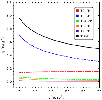
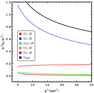
Figure 1: Pion (left) and Kaon (right) form factors calculated in the PQCD approach.

As listed in Table 2, we compare our PQCD predictions with the LCSRs results ff-pion-LCSRs ; BijnensMG at the energy point $Q^{2}=10\,\mathrm{GeV}^{2}$, where the theoretical error in our calculation mainly comes from the input of the DAs, the two sources of uncertainty in LCSRs approach are the DAs inputs and the parameters of the approach itself. The choice of the scale for the nonperturative parameters affects weakly in the larger energy regions so we do not consider it here. We find that the prediction of the pion and kaon form factors is comparable in the chosen energy point within the uncertainty, and the difference between the numerical results obtained in these two approaches becomes smaller when $Q^{2}$ is increasing.

Table 2: The PQCD and LCSRs predictions for the values of $Q^{2}F_{\pi,K}(Q^{2})$ at the point $Q^{2}=10\,\mathrm{GeV}^{2}$.

$Q^{2}(\mathrm{GeV^{2}})$	$Q^{2}F^{\mathrm{PQCD}}_{\pi}(Q^{2})$	$Q^{2}F_{\pi}^{\mathrm{LCSRs}}(Q^{2})$	$Q^{2}F_{K}^{\mathrm{PQCD}}(Q^{2})$	$Q^{2}F^{\mathrm{LCSRs}}_{K}(Q^{2})$
$10$	$0.75(10)$	$0.51(15)$	$1.08(15)$	$0.76(22)$

V Conclusion

We study the pion and kaon electromagnetic form factors with the inclusion of the high power contributions up to twist-4 of the meson DAs, the PQCD calculation confirms the convergence behaviour of the twist expansion, which shows that the contribution from the three-parton Fock state is at least one order of magnitude smaller than that from the lowest Fock state. The chiral enhancement of the subleading power contribution depends strongly on the corresponding DAs, and this effect is quite obvious in our choice of the conformal expansion of twist-3 DAs. The direct comparison between the contributions to the pion and kaon form factors from the two-parton-to-two-parton scattering indicates that the $\mathrm{SU(3)}$ asymmetry is no more than $30\%$ in the considered energy region. Because the current lattice QCD evaluation and experiment measurement of the meson form factors are still in the small $Q^{2}$ region, our calculation can not interplay directly with them now, we look forward to see more data in the intermediate energy regions at Jefferson Lab with the $12\,\mathrm{GeV}$ upgrade program, with which the precise PQCD predictions presented in this paper can be forwarded to extract the nonperturbative parameters of meson DAs, i.e., the moments in Gegenbauer expansion. We compare our results with the predictions from the LCSRs approach at the fixed energy point, and find the parallel prediction power of these two approaches. The further improvement in this project is to combine the precise measurement of the time-like pion and kaon form factors in the resonance energy regions with the PQCD calculation at the large energy regions, in order to determine the meson distribution amplitudes.

VI ACKNOWLEDGEMENTS

We are grateful to Hsiang-nan Li, Yu-ming Wang, Zhen-jun Xiao and Yi-bo Yang for helpful discussions, and especially to Hsiang-nan Li and Zhen-jun Xiao for the careful reading of the manuscript. This work is supported by the National Science Foundation of China under No. 11805060 and ”the Fundamental Research Funds for the Central Universities” under No. 531118010176.

Appendix A Definition of the distribution amplitudes

Light-cone distribution amplitudes (LCDAs) for pseudoscalar meson with quark-antiquark assignment is defined by the nonlocal matrix element sandwiched between the meson state and vacuum BallWN ; BallJE ,

$$\big{\langle}0\big{|}\overline{u}(z_{2})(\gamma_{\rho}\gamma_{5})q(z_{1})\big{|}\mathcal{P}^{-}(p)\big{\rangle}$$

$$= f_{\mathcal{P}}\int_{0}^{1}dx\,e^{-ixpz_{1}-i\overline{x}pz_{2}}\Big{\{}ip_{\rho}\left[\varphi_{\mathcal{P}}(x)+(z_{1}-z_{2})^{2}g_{1\mathcal{P}}(x)\right]+\left[(z_{1}-z_{2})_{\rho}-\frac{p_{\rho}(z_{1}-z_{2})^{2}}{p(z_{1}-z_{2})}\right]g_{2\mathcal{P}}(x)\Big{\}}\,,$$

$$\big{\langle}0\big{|}\overline{u}(z_{2})(\sigma_{\tau\tau^{\prime}}\gamma_{5})q(z_{1})\big{|}\mathcal{P}^{-}(p)\big{\rangle}$$

$$= f_{\mathcal{P}}m_{0}^{\mathcal{P}}\int_{0}^{1}dx\,e^{-ixpz_{1}-i\overline{x}pz_{2}}\left(1-\frac{m_{\pi}^{2}}{(m^{0}_{\mathcal{P}})^{2}}\right)\left[p^{\tau}(z_{1}-z_{2})_{\tau^{\prime}}-p^{\tau^{\prime}}(z_{1}-z_{2})_{\tau}\right]\,\varphi_{\mathcal{P}}^{\sigma}(x)\,,$$ (43)

$$\big{\langle}0\big{|}\overline{u}(z_{2})(i\gamma_{5})q(z_{1})\big{|}\mathcal{P}^{-}(p)\big{\rangle}=f_{\mathcal{P}}m_{0}^{\mathcal{P}}\int_{0}^{1}dx\,e^{-ixpz_{1}-i\overline{x}pz_{2}}\varphi_{\mathcal{P}}^{P}(x)\,,$$

where $f_{\mathcal{P}}$ is the decay constant, $m_{0}^{\mathcal{P}}$ is the chiral mass of the pseudoscalar meson, $\varphi_{\mathcal{P}}$, $\varphi^{P,\sigma}_{\mathcal{P}}$ and $g_{1\mathcal{P},2\mathcal{P}}$ corresponds to the DAs at twist-2, twist-3 and twist-4, respectively.

For the quark-antiquark-gluon assignment, the DAs are defined with the matrix element with the gluon field strength tensor operator $G_{\kappa\kappa^{\prime}}=g_{s}G_{\kappa\kappa^{\prime}}^{a}\lambda^{a}/2$,

$$p^{+}\big{\langle}0\big{|}\overline{u}(z_{2})(\sigma_{\tau\tau^{\prime}}\gamma_{5})G_{\kappa\kappa^{\prime}}(z_{0})q(z_{1})\big{|}\mathcal{P}^{-}(p)\big{\rangle}$$

$$= if_{3\mathcal{P}}\int\mathcal{D}x_{i}\,e^{-ix_{1}pz_{1}-ix_{2}pz_{2}-ix_{3}z_{0}}\left[\left(p_{\kappa}p_{\tau}g_{\kappa^{\prime}\tau^{\prime}}-p_{\kappa^{\prime}}p_{\tau}g_{\kappa\tau^{\prime}}\right)-\left(p_{\kappa}p_{\tau^{\prime}}g_{\kappa^{\prime}\tau}-p_{\kappa^{\prime}}p_{\tau^{\prime}}g_{\kappa\tau}\right)\right]\varphi_{3\mathcal{P}}(x_{i})\,,$$

$$p^{+}\big{\langle}0\big{|}\overline{u}(z_{2})(\gamma_{\rho}\gamma_{5})G_{\kappa\kappa^{\prime}}(z_{0})q(z_{1})\big{|}\mathcal{P}^{-}(p)\big{\rangle}$$

$$= f_{\mathcal{P}}\int\mathcal{D}x_{i}\,e^{-ix_{1}pz_{1}-ix_{2}pz_{2}-ix_{3}z_{0}}\left[p_{\rho}\frac{p_{\kappa}(z_{1}-z_{2})_{\kappa^{\prime}}-p_{\kappa^{\prime}}(z_{1}-z_{2})_{\kappa}}{p(z_{1}-z_{2})}\varphi_{\parallel}(x_{i})+(g^{\perp}_{\rho\kappa}p_{\kappa^{\prime}}-g^{\perp}_{\rho\kappa^{\prime}}p_{\kappa})\varphi_{\perp}(x_{i})\right]\,,$$

$$p^{+}\big{\langle}0\big{|}\overline{u}(z_{2})(\gamma_{\rho})\tilde{G}_{\kappa\kappa^{\prime}}(z_{0})q(z_{1})\big{|}\mathcal{P}^{-}(p)\big{\rangle}$$

$$= f_{\mathcal{P}}\int\mathcal{D}x_{i}\,e^{-ix_{1}pz_{1}-ix_{2}pz_{2}-ix_{3}z_{0}}\left[p_{\rho}\frac{p_{\kappa}(z_{1}-z_{2})_{\kappa^{\prime}}-p_{\kappa^{\prime}}(z_{1}-z_{2})_{\kappa}}{p(z_{1}-z_{2})}\tilde{\varphi}_{\parallel}(x_{i})+(g^{\perp}_{\rho\kappa}p_{\kappa^{\prime}}-g^{\perp}_{\rho\kappa^{\prime}}p_{\kappa})\tilde{\varphi}_{\perp}(x_{i})\right]\,,$$ (46)

where $\tilde{G}_{\kappa\kappa^{\prime}}=1/2\,\epsilon_{\kappa\kappa^{\prime}\eta\eta^{\prime}}G^{\eta\eta^{\prime}}$, the location of gluon file strength is at $z_{0}=vz_{1}+\overline{v}z_{2}$ with the free variable $v\in[0,1]$, $\varphi_{3\mathcal{P}}$ is the twist-3 DA, and $\varphi_{\parallel,\perp},\tilde{\varphi}_{\parallel,\perp}$ are twist-4 DAs. When $q=d,s$, the meson $\mathcal{P}=\pi,K$, respectively.

Appendix B Expressions of the distribution amplitudes

LCDAs can be obtained by using the conformal partial expansion, and the most familiar expression is the leading twist DAs written in terms of the Gegenbauer polynomials,

$$\varphi_{\mathcal{P}}(x,\mu)=6x\bar{x}\sum_{n=0}\,a_{n}(\mu)\,C_{n}^{3/2}(2x-1)\,.$$ (47)

Two-particle twist-3 DAs are related to the three-particle DA $\varphi_{3\mathcal{P}}(x_{i})$ and also to the leading twist DA $\varphi_{\mathcal{P}}$ by the QCD equation of motion (EOM), the parameter $\rho^{\mathcal{P}}=(m_{u}+m_{q})/m_{0}^{\mathcal{P}}$ is introduced to reflect the quark masses terms in the EOM, in our calacultion we only take into account the strange quark mass, with neglecting the $u,d$ quark masses unless in the chiral masses $m_{0}^{\mathcal{P}}$. To next-to-leading order in conformal spin and to the second moments in truncated conformal expansion of $\varphi_{\mathcal{P}}$, we get

$$\varphi_{\mathcal{P}}^{P}(x,\mu) = 1+3\rho^{\mathcal{P}}\Big{(}1-3a_{1}^{\mathcal{P}}+6a_{2}^{\mathcal{P}}\Big{)}(1+\ln x)-\frac{\rho^{\mathcal{P}}}{2}\Big{(}3-27a_{1}^{\mathcal{P}}+54a_{2}^{\mathcal{P}}\Big{)}\,C_{1}^{1/2}(2x-1)$$ (48)

$$+ 3\Big{(}10\eta_{3\mathcal{P}}-\rho^{\mathcal{P}}(a_{1}^{\mathcal{P}}-5a_{2}^{\mathcal{P}})\Big{)}\,C_{2}^{1/2}(2x-1)+\Big{(}10\eta_{3\mathcal{P}}\lambda_{3\mathcal{P}}-\frac{9}{2}\rho^{\mathcal{P}}a_{2}^{\mathcal{P}}\Big{)}\,C_{3}^{1/2}(2x-1)$$

$$- 3\eta_{3\mathcal{P}}\omega_{3\mathcal{P}}\,C_{4}^{1/2}(2x-1)\,,$$

$$\varphi_{\mathcal{P}}^{\sigma}(x,\mu) = 6x(1-x)\Big{\{}1+\frac{\rho^{\mathcal{P}}}{2}\Big{(}2-15a_{1}^{\mathcal{P}}+30a_{2}^{\mathcal{P}}\Big{)}+\rho^{\mathcal{P}}\Big{(}3a_{1}^{\mathcal{P}}-\frac{15}{2}a_{2}^{\mathcal{P}}\Big{)}\,C_{1}^{3/2}(2x-1)$$ (49)

$$+ \frac{1}{2}\Big{(}\eta_{3\mathcal{P}}(10-\omega_{3\mathcal{P}})+3\rho^{\mathcal{P}}a_{2}^{\mathcal{P}}\Big{)}\,C_{2}^{3/2}(2x-1)+\eta_{3\mathcal{P}}\lambda_{3\mathcal{P}}\,C_{3}^{3/2}(2x-1)$$

$$+ 3\rho^{\mathcal{P}}\Big{(}1-3a_{1}^{\mathcal{P}}+6a_{2}^{\mathcal{P}}\Big{)}\,\ln x\Big{\}}\,,$$

$$\varphi_{3\mathcal{P}}(x_{i}) = 360x_{1}x_{2}x_{3}^{2}\Big{\{}1+\lambda_{3\mathcal{P}}(x_{1}-x_{2})+\omega_{3\mathcal{P}}\frac{1}{2}(7x_{3}-3)\Big{\}}\,,$$ (50)

where the contributions from the three-particle and from the two-particle by EOM are separated clearly, the three parameters $f_{3\mathcal{P}},\lambda_{3\mathcal{P}},\omega_{3\mathcal{P}}$ can be defined by the matrix element of local twist-3 operators, and their evolution have the mixing terms with the quark mass BallWN .

For the two-particle twist-4 DAs, the definition considered in the strictly light-cone expansion in Eq. (A) is more convenient to be used in the QCD calculation, and their relations to the invariant amplitudes $\psi_{4\mathcal{P}},\phi_{4\mathcal{P}}$ defined in the Lorentz structure are,

$$g_{2\mathcal{P}}(x)=-\frac{1}{2}\int_{0}^{x}dx^{\prime}\psi_{4\mathcal{P}}(x^{\prime})\,,\,\,\,\,\,g_{1\mathcal{P}}(x)=\frac{1}{16}\phi_{4\mathcal{P}}(x)+\int_{0}^{x}dx^{\prime}g_{2\mathcal{P}}(x^{\prime})\,.$$ (51)

The relations between different operators by EOM indicate that these Lorentz invariant amplitudes are written in terms of the ”genuine” twist-4 contribution from the three-particle DAs $\varphi_{\parallel}(x_{i}),\varphi_{\perp}(x_{i})$ and the Wandzura-Wilczek-type mass corrections from the two-particle lower twist DAs, distinguishing by parameters $\delta_{\mathcal{P}}^{2}$ and $m_{\mathcal{P}}^{2}$, respectively. The corrected expressions are KhodjamirianYS

$$\psi_{4\mathcal{P}}(x) = \delta_{\mathcal{P}}^{2}\Big{[}\frac{20}{3}\,C_{2}^{1/2}(2x-1)+\frac{49}{2}a_{1}^{\mathcal{P}}\,C_{3}^{1/2}(2x-1)\Big{]}$$ (52)

$$+ m_{\mathcal{P}}^{2}\Big{\{}6\rho^{\mathcal{P}}\Big{(}1-3a_{1}^{\mathcal{P}}+6a_{2}^{\mathcal{P}}\Big{)}\,C_{0}^{1/2}(2x-1)$$

$$- \Big{[}\frac{18}{5}a_{1}^{\mathcal{P}}+3\rho^{\mathcal{P}}\Big{(}1-9a_{1}^{\mathcal{P}}+18a_{2}^{\mathcal{P}}\Big{)}+12\kappa_{4\mathcal{P}}\Big{]}\,C_{1}^{1/2}(2x-1)$$

$$+ \Big{[}2-6\rho^{\mathcal{P}}\Big{(}a_{1}^{\mathcal{P}}-5a_{2}^{\mathcal{P}}\Big{)}+60\eta_{3\mathcal{P}}\Big{]}\,C_{2}^{1/2}(2x-1)$$

$$+ \Big{(}\frac{18}{5}a_{1}^{\mathcal{P}}-9\rho^{\mathcal{P}}a_{2}^{\mathcal{P}}+\frac{16}{3}\kappa_{4\mathcal{P}}+20\eta_{3\mathcal{P}}\lambda_{3\mathcal{P}}\Big{)}\,C_{3}^{1/2}(2x-1)$$

$$+ \Big{(}\frac{9}{4}a_{2}^{\mathcal{P}}-6\eta_{3\mathcal{P}}\omega_{3\mathcal{P}}\Big{)}\,C_{4}^{1/2}(2x-1)\Big{\}}$$

$$+ 6m_{q}^{2}\Big{(}1-3a_{1}^{\mathcal{P}}+6a_{2}^{\mathcal{P}}\Big{)}\,\ln x\,,$$

$$\phi_{4\mathcal{P}}(x) = \delta_{\mathcal{P}}^{2}\Big{\{}\Big{(}\frac{200}{3}+196(2x-1)a_{1}^{\mathcal{P}}\Big{)}x^{2}\bar{x}^{2}$$ (53)

$$+ 21\omega_{4\mathcal{P}}\Big{(}x\bar{x}(2+13x\bar{x})+[2x^{3}(6x^{2}-15x+10)\ln x]+[x\leftrightarrow\bar{x}]\Big{)}$$

$$- 14a_{1}^{\mathcal{P}}\Big{(}x\bar{x}(2x-1)(2-3x\bar{x})-[2x^{3}(x-2)\ln x]+[x\leftrightarrow\bar{x}]\Big{)}\Big{\}}$$

$$+ m_{\mathcal{P}}^{2}\Big{\{}\frac{16}{3}\kappa_{4\mathcal{P}}\Big{(}x(2x-\bar{x})(1-2x\bar{x})+[5(x-2)x^{3}\ln x]-[x\leftrightarrow\bar{x}]\Big{)}$$

$$+ 4\eta_{3\mathcal{P}}x\bar{x}\Big{[}60\bar{x}+10\lambda_{3\mathcal{P}}\Big{(}(2x-1)(1-x\bar{x})-(1-5x\bar{x})\Big{)}$$

$$- \omega_{3\mathcal{P}}\Big{(}3-21x\bar{x}+28x^{2}\bar{x}^{2}+3(2x-1)(1-7x\bar{x})\Big{)}\Big{]}$$

$$- \frac{36}{5}a_{2}^{\mathcal{P}}\Big{(}\frac{1}{4}x\bar{x}(4-9x\bar{x}+110x^{2}\bar{x}^{2})+[x^{3}(10-15x+6x^{2})\ln x]+[x\leftrightarrow\bar{x}]\Big{)}$$

$$+ 4x\bar{x}(1+3x\bar{x})\Big{(}1+\frac{9}{5}(2x-1)a_{1}^{\mathcal{P}}\Big{)}\Big{\}}\,,$$

with $\eta_{3\mathcal{P}}=f_{3\mathcal{P}}/(f_{\mathcal{P}}m_{0}^{\mathcal{P}})$. It is noticed in Eq. (52) that $\psi_{4\mathcal{P}}(x)$ has a logarithm end-point singularity for the finite quark mass, while this singularity is not existed in $\phi_{4\mathcal{P}}(x)$. The conformal expansion of three-particle twist-4 DAs reads:

$$\psi_{\parallel}(x_{i}) = 120x_{1}x_{2}x_{3}\Big{\{}\delta_{\mathcal{P}}^{2}\Big{[}\frac{21}{8}(x_{1}-x_{2})\omega_{4\mathcal{P}}+\frac{7}{20}a_{1}^{\mathcal{P}}(1-3x_{3})\Big{]}$$ (54)

$$\hskip 42.67912pt+m_{\mathcal{P}}^{2}\Big{[}-\frac{9}{20}(x_{1}-x_{2})a_{2}^{\mathcal{P}}+\frac{1}{3}\kappa_{4\mathcal{P}}\Big{]}\Big{\}}\,,$$

$$\psi_{\perp}(x_{i}) = 30x^{2}_{3}\Big{\{}\delta_{\mathcal{P}}^{2}\Big{[}\frac{1}{3}(x_{1}-x_{2})+\frac{7}{10}a_{1}^{\mathcal{P}}\Big{(}-x_{3}(1-x_{3})+3(x_{1}-x_{2})^{2}\Big{)}+\frac{21}{4}\omega_{4\mathcal{P}}(x_{1}-x_{2})(1-2x_{3})\Big{]}$$ (55)

$$\hskip 17.07182pt+m_{\mathcal{P}}^{2}(1-x_{3})\Big{[}\frac{9}{40}(x_{1}-x_{2})-\frac{1}{3}\kappa_{4\mathcal{P}}\Big{]}\Big{\}}\,,$$

$$\tilde{\psi}_{\parallel}(x_{i}) = -120x_{1}x_{2}x_{3}\delta_{\mathcal{P}}^{2}\Big{\{}\frac{1}{3}+\frac{7}{4}a_{1}^{\mathcal{P}}(x_{1}-x_{2})+\frac{21}{8}\omega_{4\mathcal{P}}(1-3x_{3})\Big{\}}\,,$$ (56)

$$\tilde{\psi}_{\perp}(x_{i}) = 30x_{3}^{2}\Big{\{}\delta_{\mathcal{P}}^{2}\Big{[}\frac{1}{3}(1-x_{3})-\frac{7}{10}a_{1}^{\mathcal{P}}(x_{1}-x_{2})(4x_{3}-3)+\frac{21}{4}\omega_{4\mathcal{P}}(1-x_{3})(1-2x_{3})\Big{]}$$ (57)

$$\hskip 17.07182pt+m_{\mathcal{P}}^{2}\Big{[}\frac{9}{40}a_{2}^{\mathcal{P}}(x_{1}^{2}-4x_{1}x_{2}+x_{2}^{2})-\frac{1}{3}(x_{1}-x_{2})\kappa_{4\mathcal{P}}\Big{]}\Big{\}}\,,$$

in which three nonperturbative parameters $\delta_{\mathcal{P}}^{2},\omega_{4\mathcal{P}},\kappa_{4\mathcal{P}}$ are introduced. We close this section by noticing that all parameters in the conformal expansion of DAs have the scale dependence and the behaviours of their evolutions can be found in Ref. BallWN .

References

• (1) G. P. Lepage and S. J. Brodsky, Phys. Rev. Lett.  43, 545 (1979), Erratum: [Phys. Rev. Lett.  43, 1625 (1979)].
• (2) G. P. Lepage and S. J. Brodsky, Phys. Rev. D 22, 2157 (1980).
• (3) A. V. Efremov and A. V. Radyushkin, Phys. Lett.  94B, 245 (1980).
• (4) T. Gousset and B. Pire, Phys. Rev. D 51, 15 (1995).
• (5) A.P. Bakulev, K. Passek-Kumericki, W. Schroers and N.G. Stefanis, Phys. Rev. D 70, 033014(2004); V.A. Nesterenko and A.V. Radyushkin, Phys. Lett. B 115, 410(1982); C.E. Carlson and J. Milana, Phys. Rev. Lett. 65, 1717(1990); B. Melic, B. Nizic and K. Passek, Phys. Rev. D 60, 074004(1999).
• (6) V. Braum and I. Halperin, Phys. Lett. B 328, 457(1994); A. Khodjamirian, arXiv:hep-ph/9909450, WUE-ITP-99-021; V.M. Braun, A. Khodjamirian and M. Maul, Phys. Rev. D 61, 073004(2000).
• (7) U. Raha and A. Aste, Phys. Rev. D 79, 034015(2009); H.N. Li, Y.L. Shen, Y.M. Wang and H. Zou, Phys. Rev. D 83, 054029(2011); S. Cheng, Y.Y. Fan and Z.J. Xiao, Phys. Rev. D 89, 054015(2014).
• (8) F.D.R. Bonnet, R.G. Edwards, G.T. Fleming, R. Lewis and D.G. Richards, Phys. Rev. D 72,054506(2005); G.T. Fleming, F.D.R. Bonnet, R.G.Edwards, R. Lewis and D.G. Richards, Nucl. Phys. B (Proc.Suppl)140,302(2005).
• (9) C.J. Bebek, et al., (Harvard $\&$ Cornell), Phys. Rev. D 9, 1229(1974);   Phys. Rev. D 17, 1693(1978).
• (10) T.K. Pedlar, et al., (CLEO Collaboration), Phys. Rev. Lett. 95, 261803(2005).
• (11) T. Horn, et al., (Jefferson Lab $F_{\pi}$ Collaboration), Phys. Rev. Lett. 97, 192001(2006);
• (12) M. Beneke, G. Buchalla, M. Neubert and C. T. Sachrajda, Phys. Rev. Lett.  83, 1914 (1999); Nucl. Phys. B 591, 313 (2000); Nucl. Phys. B 606, 245 (2001).
• (13) C. W. Bauer, S. Fleming and M. E. Luke, Phys. Rev. D 63, 014006 (2000); C. W. Bauer, S. Fleming, D. Pirjol and I. W. Stewart, Phys. Rev. D 63, 114020 (2001).
• (14) M. Beneke, A. P. Chapovsky, M. Diehl and T. Feldmann, Nucl. Phys. B 643, 431 (2002); M. Beneke and T. Feldmann, Phys. Lett. B 553, 267 (2003).
• (15) H. n. Li and H. L. Yu, Phys. Rev. D 53, 2480 (1996); H. n. Li, Phys. Rev. D 52, 3958 (1995); T. W. Yeh and H. n. Li, Phys. Rev. D 56, 1615 (1997); H. n. Li and B. Tseng, Phys. Rev. D 57, 443 (1998); C. D. Lu, K. Ukai and M. Z. Yang, Phys. Rev. D 63, 074009 (2001); A. Ali, G. Kramer, Y. Li, C. D. Lu, Y. L. Shen, W. Wang and Y. M. Wang, Phys. Rev. D 76, 074018 (2007); Q. Qin, Z. T. Zou, X. Yu, H. n. Li and C. D. Lü, Phys. Lett. B 732, 36 (2014); W. Bai, M. Liu, Y. Y. Fan, W. F. Wang, S. Cheng and Z. J. Xiao, Chin. Phys. C 38, 033101 (2014).
• (16) V. M. Belyaev, V. M. Braun, A. Khodjamirian and R. Ruckl, Phys. Rev. D 51, 6177 (1995).
• (17) J. Bijnens and A. Khodjamirian, Eur. Phys. J. C 26, 67 (2002).
• (18) Y. C. Chen and H. n. Li, Phys. Rev. D 84, 034018 (2011).
• (19) H. n. Li, Y. L. Shen and Y. M. Wang, Phys. Rev. D 85, 074004 (2012).
• (20) S. Cheng, Y. Y. Fan and Z. J. Xiao, Phys. Rev. D 89, 054015 (2014).
• (21) J. Botts and G. F. Sterman, Nucl. Phys. B 325, 62 (1989).
• (22) H. n. Li and G. F. Sterman, Nucl. Phys. B 381, 129 (1992).
• (23) F. g. Cao, T. Huang and C. w. Luo, Phys. Rev. D 52, 5358 (1995).
• (24) S. Cheng and Q. Qin, Phys. Rev. D 99, 016019 (2019).
• (25) M. Tanabashi et al. [Particle Data Group], Phys. Rev. D 98, 030001 (2018).
• (26) G. F. Sterman, Nucl. Phys. B 281, 310 (1987).
• (27) S. Catani and L. Trentadue, Nucl. Phys. B 327, 323 (1989).
• (28) H. n. Li, Phys. Rev. D 55, 105 (1997).
• (29) Y. Y. Keum, H. N. Li and A. I. Sanda, Phys. Rev. D 63, 054008 (2001).
• (30) Y. Y. Keum, H. n. Li and A. I. Sanda, Phys. Lett. B 504, 6 (2001).
• (31) H. n. Li and Y. M. Wang, JHEP 1506, 013 (2015).
• (32) Y. M. Wang, EPJ Web Conf.  112, 01021 (2016).
• (33) J. Collins, Foundations of Perturbative QCD, Cambridge Monographs on Particle Physics, Nuclear Physics, and Cosmology, 32, ISBN: 9780521855334.
• (34) H. N. Li, Y. L. Shen and Y. M. Wang, JHEP 1401, 004 (2014).
• (35) Y. L. Shen, Z. T. Zou and Y. Li, [arXiv:1901.05244 [hep-ph]].
• (36) H. C. Hu and H. n. Li, Phys. Lett. B 718, 1351 (2013).
• (37) S. Cheng and Z. J. Xiao, Phys. Lett. B 749, 1 (2015).
• (38) S. Cheng, Z. J. Xiao and Y. L. Zhang, Nucl. Phys. B 896, 255 (2015).
• (39) J. Hua, S. Cheng, Y. l. Zhang and Z. J. Xiao, Phys. Rev. D 97, 113002 (2018).
• (40) Y. L. Zhang, J. Hua, Z. C. Ji and Z. J. Xiao, [arXiv:1811.10204 [hep-ph]].
• (41) H. Leutwyler, Phys. Lett. B 378, 313 (1996).
• (42) A. Khodjamirian, C. Klein, T. Mannel and N. Offen, Phys. Rev. D 80, 114005 (2009).
• (43) G. S. Bali et al., [RQCD Collaboration] [arXiv:1903.08038 [hep-lat]].
• (44) V. M. Braun and I. E. Filyanov, Z. Phys. C 48, 239 (1990), [Sov. J. Nucl. Phys.  52, 126 (1990)], [Yad. Fiz.  52, 199 (1990)].
• (45) P. Ball, V. M. Braun and A. Lenz, JHEP 0605, 004 (2006).
• (46) V. A. Novikov, M. A. Shifman, A. I. Vainshtein, M. B. Voloshin and V. I. Zakharov, Nucl. Phys. B 237, 525 (1984).
• (47) A. P. Bakulev, S. V. Mikhailov and N. G. Stefanis, Phys. Rev. D 67, 074012 (2003).
• (48) G. S. Bali et al. [RQCD Collaboration], Phys. Lett. B 774, 91 (2017).
• (49) G. S. Bali et al. [RQCD Collaboration], Eur. Phys. J. C 78, 217 (2018).
• (50) G. S. Bali et al. [RQCD Collaboration], Phys. Rev. D 98, 094507 (2018).
• (51) P. Ball, JHEP 9901, 010 (1999).