Soft X-ray heating as a mechanism of optical continuum generation in solar-type star superflares

Abstract

Superflares on the solar type stars observed by Kepler demonstrate the contrast in the optical continuum of the order 0.1–1 per cent. The mechanism of formation of this radiation is not firmly established. We consider a model where the stellar atmosphere is irradiated by the soft X rays emitted from the flaring loop filled with the hot plasma. This radiation heats a large area beneath the loop. Subsequent cooling due to h^- and hydrogen free-bound emission can contribute to the observed enhanced continuum. We solve the equations of radiative transfer, statistical equilibrium, ionization balance and radiative equilibrium in the model atmosphere illuminated by the soft X rays, compute the temperature and the electron density in the atmosphere and find the emergent radiation. We found that a flare loop of the length $\sim 10^{10}$ cm and plasma density $10^{12}$ cm^-3 at the temperature $T=20$ MK can provide the contrast in the Kepler bandpass of 0.1 and 0.8 per cent if the heated region covers $\sim$ 1 and 10 per cent of the visible stellar surface respectively. The required emission measure is of the order $10^{55}$ cm^-3.

1 Introduction

Flaring stars are observed across HR diagram (Pettersen, 1989; Balona, 2015). Among main sequence stars, flares are most commonly observed on UV Cet type stars which are M dwarfs with emission lines (dMe type). Flares on hotter stars, in particular G stars, have been reported more rarely. This can be attributed to the fact that, on brighter stars, only sufficiently powerful flares can be detected. Moreover, such stars probably flare less frequently.

Observations of flares on G stars were hugely enriched by the Kepler mission (Borucki et al., 2010) which continuously observed more than 150000 stars for four years with exceptional photometric accuracy. Maehara et al. (2012) reported on 365 superflares on 148 solar-type stars observed in 120 days. Shibayama et al. (2013) extended this result to 1547 flares. The spectral band of Kepler is from 4000 to 9000 Å and the contrast of the flares in such a wide range (essentially, in white light) is itself striking: the typical value is 1 per cent of the average non-flaring brightness, but sometimes it can reach even 10 per cent. Solar white light flares can provide a contrast of only 0.01 per cent when integrated over the disc (Haisch et al., 1991). On the other hand, flares on M dwarfs can easily increase the brightness of the star by many times, e.g., two flares on UV Cet had $U$-band contrast of 8.2 and 127.1 (Bopp & Moffett, 1973), a flare on EV Lac had $\Delta U=3.62$, i.e. the $U$-band contrast 28 (Alekseev et al., 1994). Pettersen (2016) observed a $\Delta U=7.2$ flare on EV Lac and Hawley & Pettersen (1991) observed a $\Delta U=4.5$ flare on AD Leo. See also multiwavelength observations of a giant flare on CN Leo by Fuhrmeister et al. (2008) and a comprehensive overview by Gershberg (2005).

However, M dwarfs differ from solar-type stars in that they are fainter (hence flares are relatively more prominent), smaller (hence flare photospheric filling factor can be larger) and have somewhat different structure of the atmosphere due to lower $T_{\mathrm{eff}}$ and larger $\log g$. Therefore one can ask whether and to what extent the mechanisms of radiation are common for superfalres on dMe and solar-type stars. As Heinzel & Shibata (2018) noted in regard to the results of Maehara et al. (2012), ‘only a limited attention was devoted to understanding the mechanisms of the superflare emission’.

Since the beginning of the study of solar and stellar flares, there have been proposed a number of mechanisms of heating the lower atmosphere which can result in the optical continuum emission. Najita & Orrall (1970) considered the heating of the solar atmosphere by non-thermal electrons and protons. Aboudarham & Henoux (1989) argued that the white light emission in solar flares results from heating the photosphere by the enhanced radiation of the chromosphere which in turn is heated by non-thermal electron beams. Analogous conclusions are drawn by Machado et al. (1989), but they argue that the chromospheric heating by protons is more preferable. Direct heating of the upper photosphere by non-thermal electrons and protons in case of stellar flares was discussed by Grinin & Sobolev (1977, 1988, 1989). Heating of the stellar photosphere by soft X rays from the flare loop was considered by Mullan & Tarter (1977) and, more thoroughly, by Hawley & Fisher (1992) (hereafter HF92). Livshits et al. (1981) calculated the gasdynamic response of the atmosphere to the bombardment by non-thermal electrons and proposed that the so-called low-temperature condensation can account for the optical continuum of stellar flares. The model was refined by the authors in a subsequent paper Katsova et al. (1997); the radiation hydrodynamics approach was also developed by Fisher et al. (1985); Abbett & Hawley (1999); Allred et al. (2005). Mullan (1976) proposed that the photosphere can be heated by the thermal conduction from the flaring loop filled with the hot plasma. Heinzel & Shibata (2018) argue that the continuum radiation of stellar superflares can be dominated by the flare loop radiation, especially hydrogen free-free radiation.

The mechanisms mentioned above are usually invoked to explain either impulsive or gradual phase of the flare. The light curves of the flares reported by Maehara et al. (2012) show gradual decay. In fact, these observations were conducted in the Kepler’s long cadence mode (30 min time resolution), so each flare containing several data points lasted for several hours and was gradual in nature (although the presence of an impulsive phase cannot be excluded) and the most energy in the optical range was apparently emitted in the gradual phase. In this paper we will consider heating of the photosphere by the soft X rays from the flare loop as a possible cause to the optical continuum to emerge in the gradual phase of superflares on solar-type stars. As was noted above, this mechanism has been discussed in a number of papers, but, in case of stellar flares, to our knowledge, they were always assumed to occur on M dwarfs. On the other hand, it was also considered in the context of solar flares, but for flare energies typical for the Sun. Our aim is to apply strong heating by the soft X rays to an atmosphere of a solar-type star and find out the parameters of the hot plasma which can account for the observed contrast of G-type star supeflares in the Kepler bandpass.

2 Problem setup

The general picture of stellar flares is qualitatively analogous to the standard model of solar flares. First, the energy of the non-potential magnetic field is rapidly released. Some large portion of this energy is thought to be transferred to non-thermal particles, electrons or protons. The particles travel along the magnetic field lines and impact the chromosphere. This process is usually thought to account for the impulsive phase of a flare. The impact results in a strong heating and evaporation of the chromospheric material which expands drastically at the temperature of $10^{7}-10^{8}$ K and fills the magnetic loop. Thus, the loop becomes a source of soft X rays (SXR) which irradiate the stellar surface. Our aim is to find the properties of the SXR plasma which could provide irradiation of a solar-type star so that the disc-integrated brightness in the white light increased by $\sim 1$ per cent. We do this by solving the set of the equations of radiative transfer, statistical equilibrium, ionization balance and radiative equilibrium in a stellar atmosphere irradiated by the SXR. Since we are interested in flares on solar-type stars, we use the Harvard Smithsonian reference atmosphere (Gingerich et al., 1971), or HSRA, which is a semi-empirical model of the solar photosphere and the chromosphere up to the height of 1850 km above the point $\tau_{5000}=1$.

The irradiation by SXR is included as the upper boundary condition in the equations of radiative transfer. The intensity of SXR is computed with the chianti package (Del Zanna et al., 2015).

The equations of statistical equilibrium are solved with the method of accelerated lambda iteration as implemented by Rybicki & Hummer (1992), hereafter RH92. The equation of radiative equilibrium in its simplest form reads

$$4\pi\int(\chi_{\nu}J_{\nu}-\eta_{\nu})d\nu=0$$ (1)

where $\chi_{\nu}$ is the opacity, $\eta_{\nu}$ is the emissivity and $J_{\nu}$ is the mean (i.e. angle averaged) intensity. However, as discussed by Kubát et al. (1999), this form can be not appropriate in the outer layers of the atmosphere because of decoupling of the radiation from the thermal energy reservoir of the atmospheric material. One possible solution proposed by Kubát et al. (1999) is to use the so called thermal electron balance, i.e. to write the energy conservation law as applied to the thermal energy of free electrons rather than to the energy of the radiation. However, when we applied this method in the case of strong external heating by SXR, we could not reach convergence. Therefore, we used the equation of radiative equilibrium. To avoid the difficulty of strong line scattering mentioned above, we applied the technique of the approximate lambda operator in a manner similar to that of RH92, see appendix A for details.

The whole set of equations is solved iteratively in the following way.

1. The atomic level populations and electron number densities at all the depths were assigned LTE values and the formal solution of the equation of radiative transfer was found.

2. With the radiation intensity, electron number density and the temperature fixed, the atomic level populations are found iteratively following the procedure of RH92.

3. All the equations (statistical equilibrium, ionization balance and the radiative equilibrium) are linearized with respect to the corresponding variables (atomic level populations, electron number density and temperature) and the corrections are found. However, the corrections to the level populations are discarded at this step and only electron number density and temperature are corrected. Such a strategy was reported to have a stabilizing effect by Mihalas & Auer (1970); Auer & Mihalas (1969), see also Kubat (1997).

4. With the temperature and electron density updated, opacity is recalculated and a new formal solution for the radiation is found.

5. Move to the step (ii).

This algorithm was repeated until the corrections of the level populations, electron number density and temperature were small.

In our calculations we included a 6 level + continuum H i atom, a 5 level + continuum Ca ii atom and a 6 level + continuum Mg ii atom. The oscillator strengths for hydrogen were taken from Wiese & Fuhr (2009), the bound-free opacity was calculated according to the Kramers formula with the Gaunt factors taken from Karzas & Latter (1961). The free-free opacity for hydrogen was calculated with the classical formula and a constant Gaunt factor. For Mg ii and Ca ii, oscillator strengths were taken from the VALD database (Ryabchikova et al., 2015) and the photoionization cross sections from the TOPbase project (Cunto & Mendoza, 1992; Cunto et al., 1993). Free-free opacity for Ca ii and Mg ii was calculated analogously to H i. This rough approximation is applicable because free-free processes for these atoms contribute very little to the overall opacity. The abundance of the negative hydrogen ion was calculated in LTE relative to the ground state of neutral hydrogen. Bound-free and free-free opacities for it were calculated according to Kurucz (1970).

In this work we only took into account collisions with electrons. Electron impact excitation rates were taken from Przybilla & Butler (2004) for H i, Meléndez et al. (2007) for Ca ii and Sigut & Pradhan (1995) for Mg ii. The data for the impact ionization were taken from Mihalas (1967) for H i and the Seaton formula was used for Ca ii and Mg ii (Seaton, 1962).

When calculating the electron density from the charge conservation equation, we take into account that the ionization of H i, Mg ii and Ca ii obeys the equation of statistical equilibrium; also, we include the LTE ionization of the neutral helium, carbon, oxygen, silicon and iron.

The SXR heating is enabled via ionization of hydrogen and K-shell photoionization of helium, carbon, oxygen, magnesium and silicon. The absorption cross sections in this spectral range are taken from Karzas & Latter (1961) for hydrogen and computed with the code mucal which uses the compilation of X-ray cross sections from McMaster et al. (1969) for heavy atoms. While the ionization of hydrogen is treated self-consistently, this is not the case for heavier atoms: we did not take into account the cascade transitions after K-shell ionization and corresponding radiative losses. Therefore, when computing the heating due to K-shell ionization of non-hydrogenic atoms, we only took into account the energy of the escaping electron, so that the term in the energy balance equation corresponding to the K-shell ionization reads

$$Q_{\mathrm{SXR}}=4\pi n\int_{h\nu_{0}}^{\infty}\alpha_{\nu}J_{\nu}(1-\frac{h\nu_{0}}{h\nu})d\nu$$ (2)

where $n$ is the number density of atoms of a certain element, $h\nu_{0}$ is the threshold of the K-shell ionization, $\alpha_{\nu}$ is the ionization cross section.

The intensity of the SXR was calculated in the chianti package. We chose the constant temperature of plasma to be $T=20$ MK which is quite typical for stellar flares.

Three values of the emission measure were tried: $\log\mathrm{EM}=33,34,34.5$. Note that chianti computes the column emission measure, which implies that in our model calculations, the source of SXR is represented by a box on the top of the model atmosphere homogeneously filled with the hot plasma. The height of the box $h$ and the plasma density in it $n$ are such that $n^{2}h=\mathrm{EM}$ where EM has the values indicated above. The horizontal extent of the box should be chosen so that the corresponding volume emission measure is comparable to the observed values. Our important assumption is that, if the plasma within the box is condensed into a flare loop (conserving the temperature and the volume emission measure), the irradiation and heating of the stellar surface below it does not change radically. The relation between the box size and the flare loop parameters is discussed in the next section.

HF92 found that the X rays with the wavelengths $\gtrsim 25$ Å are absorbed in the highest levels of the chromosphere. In our model, the chromosphere extends up to 1850 km and we also see that the longer wavelength X rays are absorbed at the highest levels. These levels do not contribute to the heating of the photosphere and do not produce considerable optical continuum. Moreover, strong heating of these layers makes the calculation unstable so that it can fail to converge. Therefore we assumed the SXR emission to span from 0.1 to 25 Å. Since the high resolution spectrum in this region is not of much importance to us, we smoothed it with an instrumental profile of FWHM = 3 Å to keep the frequency grid relatively coarse.

In principle, our method of solution is close to that of HF92 (except that we do not model the flaring loop itself and the transition region). The important difference is that we apply the strong heating to the solar atmosphere model and assume that it is not only the footpoint of the flaring loop which is heated by SXR, but a large area below the loop. Also, we use more detailed SXR spectrum and solve the equation of radiative equilibrium within the global iterative procedure.

3 Results and discussion

Using the techniques described in the previous section, we calculated the temperature and electron density in the atmosphere heated by the external SXR. We should note that we did not solve the equation of hydrostatic equilibrium and the heavy particle stratification was fixed. We assume that this simplification does not affect our results significantly. The temperature and electron density in the heated models are shown in Figs. 1 and 2. In these and following figures, $m$ is the mass column density in g cm^-2.

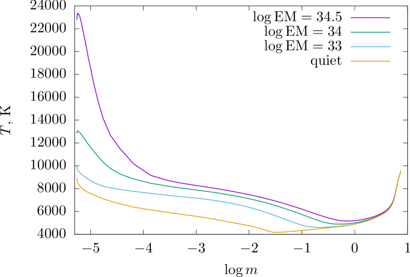
Figure 1: The temperature in the quiescent model and heated models

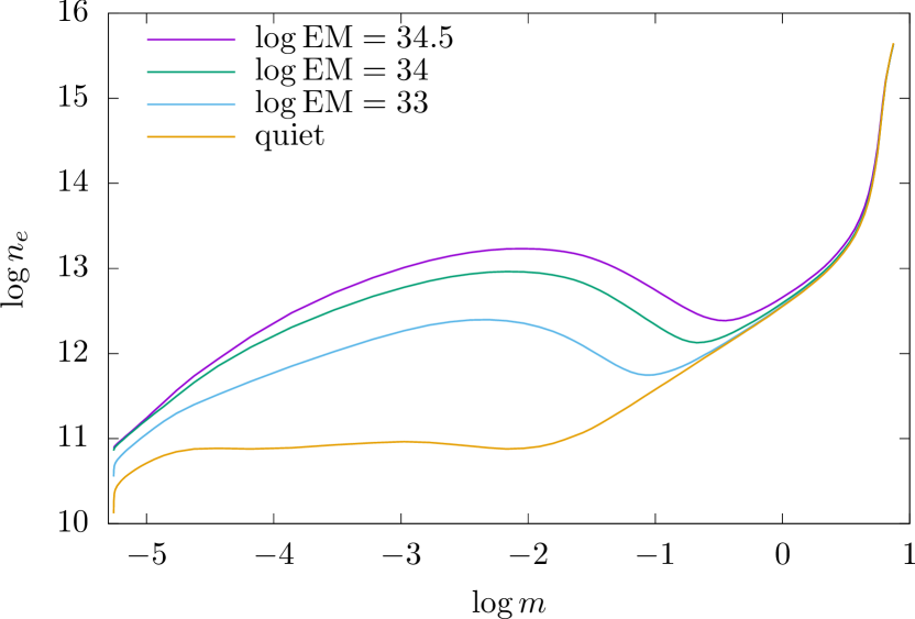
Figure 2: The electron density in the quiescent model and heated models.

One can see that all the three models can provide quite strong heating below the temperature minimum, but the maximum column depth where heating is present increases with the emission measure of the hot plasma. In the following, we will refer to the results obtained for the strongest heating ($\log\mathrm{EM}=34.5$) as the most representative case.

Fig. 3 shows the processes responsible for the heating and cooling of the irradiated atmosphere.

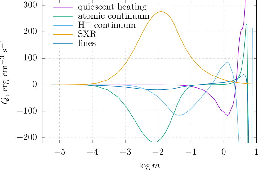
Figure 3: The contributions of various atomic processes to the overall heating (positive values) and cooling (negative values) in the model atmosphere.

Positive values correspond to heating and negative ones to cooling. The heating by SXR has a broad maximum around $\log m=-2$. Note however that the $x$ scale is logarithmic; in linear scale, the SXR heating shows abrupt rise and much slower decline with the depth. The heating shown in Fig. 3 is calculated per unit volume. Therefore, although the heating at the top of the model atmosphere is low, the temperature rise in this region is high due to the low density as can be seen in Fig. 1. Recall once again that we restricted the SXR spectrum by the limits 0.1 – 25 Å. Radiation at longer wavelengths would be absorbed in the highest levels of the atmosphere which would result in even stronger heating. Our test calculations in case of low emission measure show that this increased heating of the outer layers has small effect on the temperature of the underlying material and the overall amount of the optical continuum.

The SXR heating is balanced by the cooling due to the line emission, atomic continuum and h^- continuum. In case of relatively weak heating ($\log\mathrm{EM}=33$), the cooling is realized by the line emission (peaks at $\log m=-2.2$) and h^- emission (peaks at $\log m=-1.2$), while the contribution from the atomic continua is weak. When the emission measure and SXR heating increase, the cooling rate due to h^- increases accordingly, while the line cooling grows slowly and cooling due to atomic continuum processes becomes more important. In case of $\log\mathrm{EM}=34.5$ (Fig. 3) line cooling is about one tenth of atomic continuum cooling. The main components of this continuum are Balmer and, to a lesser extent, Paschen continua. The cooling feature arises because, due to the enhanced temperature, spontaneous bound-free emission dominates over the photoabsorption. In deeper layers, the temperature goes down, and both hydrogen second level population and ionization degree become lower, so that both heating and cooling decrease. In these layers cooling is due to h^- bound-free emission.

HF92 found that the atmosphere is heated not only directly by the SXR, but also by the hydrogen free-bound emission arising from the regions heated by SXR, the effect predicted for the Sun by Avrett et al. (1986). In our calculations, we do not see significant heating below the temperature minimum region due to hydrogen free-bound emission. This heating is still caused by the shortest wavelength SXR penetrating to such deep layers.

In figure 1 of HF92, one can see that the quiescent heating is not zero, but has a minimum around $\log m=0$ followed by a larger maximum. The authors attribute this maximum to the fact that the model they used included convective heating, while they took into account only radiative heating and cooling. Our model has similar features, but they are larger in absolute value. We suppose that the interpretation of HF92 is applicable in our case since Gingerich et al. (1971) tried to take the convection into account when constructing HSRA.

External heating of the atmosphere affects the emergent radiation spectrum. We found that the contrast, i.e. the ratio of the emergent intensity from the heated atmosphere to that of the quiescent atmosphere, strongly depends on the viewing angle. In other words, it depends on the location of the heated region on the stellar disc: in the center of the disc, the contrast is smaller while near the limb it is larger. Spectra of the heated and quiescent models for the two locations of the flaring region are shown in Fig. 4.

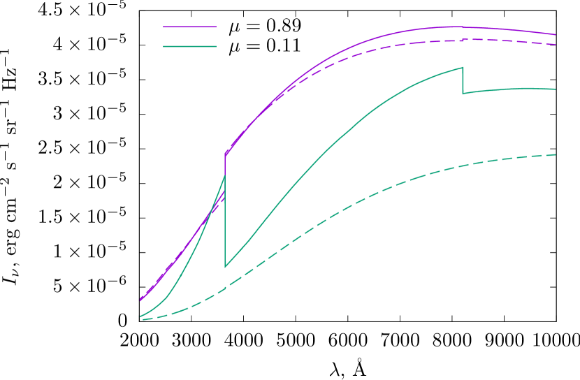
Figure 4: The continuum spectra of the radiation from the heated model atmosphere for the two viewing angles. Dashed lines represent the quiescent spectrum. The hot plasma emission measure is $\log\mathrm{EM}=34.5$.

We computed the contribution functions for Paschen continuum and h^- free-bound emission at the reference wavelength of 5000 Å according to Magain (1986):

$$C=\frac{\ln 10}{\mu}\frac{\eta}{\chi}\tau_{5000}e^{-\tau_{5000}/\mu}$$ (3)

where $\eta$ is the h^- or Paschen free-bound emissivity, $\chi$ is the total absorption (both taken at 5000 Å), $\tau_{5000}$ is the optical depth at 5000 Å, $\mu=\cos\theta$ is the cosine of the viewing angle. Fig. 5 shows the contribution functions for the more representative case of $\mu=0.11$ (close to the limb).

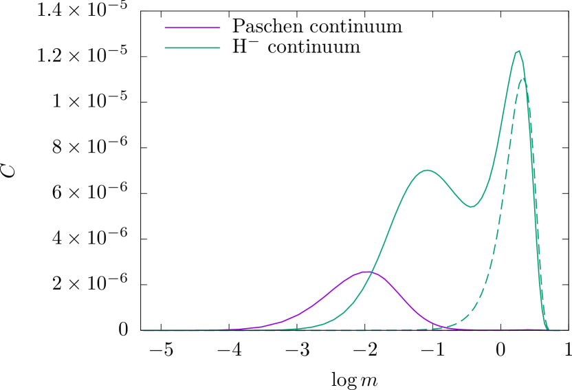
Figure 5: Contribution functions for Paschen and h^- free-bound emission. Dashed lines correspond to the quiet atmosphere. The hot plasma emission measure is $\log\mathrm{EM}=34.5$ and the viewing angle cosine is $\mu=0.11$

Dashed lines correspond to the quiescent atmosphere. One can see that Paschen continuum does contribute to the overall intensity, but the main contribution is due to h^- and comes from deeper layers. However, the significant enhancement of the h^- emission around $\log m=-1$ is located substantially higher in the atmosphere than the region from which the bulk optical continuum emerges. This allows to explain the dependence of the contrast on the viewing angle on the basis of the Eddington-Barbier relation [see Mihalas (1978)]. At the disk center we see the bright radiation of the photosphere and the excess radiation of the heated region is lost in it. When approaching the limb, the photospheric radiation becomes suppressed and the heated region contributes relatively more to the overall intensity.

For decades of observations of stellar flares and solar white light flares (WLFs) there has been a debate about the depth and mechanism of the optical continuum formation. Avrett et al. (1986) argue that the optical continuum can be due to the hydrogen free-bound emission from the overheated upper chromosphere. However they note that this same emission can also heat temperature minimum region and cause the h^- radiation to emerge. The idea of backwarming was used by Isobe et al. (2007) to interpret the morphology of white light emitting patches in an X class solar flare. They found that the region of backwarming is located 100 km below (i.e. very close to) the region of the primary heating. The latter is associated with the region where non-thermal electrons deposit their energy. In the model atmosphere we used, 20 keV electrons stop at $\log m=-4$ (Syrovatskii & Shmeleva, 1972), high above the temperature minimum region. 100 keV electrons stop at $\log m=-2.5$, close to the depth where we obtained the maximum hydrogen continuum cooling. However, the electron spectrum should be rather hard in order for the bulk energy to be contained in such energetic particles. Or, alternatively, heating by protons should be invoked. Note also that the region heated by non-thermal electrons emits in extreme ultraviolet while we considered irradiation by soft X rays. Therefore the two models are probably not directly comparable. Also, to interpret the gradual decay phase with the backwarming mechanism, one has to assume continuous precipitation of the non-thermal particles as is the case in solar two-ribbon flares. In our model, we assume that there is no sustained heating when the loop is filled with the hot plasma.

In a recent work, Heinzel et al. (2017) report the observations of a white light emission in an off-limb solar flare coming from the height of $\sim 1000$ km which they attribute to the Paschen continuum. On the other hand, Martínez Oliveros et al. (2012) report the observations of white light emission from as low as 200–400 km above the photosphere. Moreover, there are observations of WLFs with weak Balmer continuum (Hiei, 1982; Boyer et al., 1985); Fang & Ding (1995) discuss the two types of solar WLFs supporting either hydrogenic or h^- origin of the optical continuum. In case of stellar flares, the identification of the optical continuum origin is even harder. To our knowledge, photometric and spectral observations are available only for flares on dMe stars [see e.g. Kowalski et al. (2013) and references therein] and for solar-type stars we only have to rely on the models. In our calculations we see that the cooling of the region above the temperature minimum (at $\log m\sim-2$) due to the hydrogen recombination is partly responsible for the optical continuum generation, but the main contribution is from h^- free-bound radiation emerging from below the temperature minimum region ($\log m\sim-1$). One should also remember that Kepler is completely insensitive to the Balmer continuum which therefore is excluded from possible causes of the flare contrasts reported by Maehara et al. (2012).

As was mentioned above, the contrast in the specific intensity grows from the disc center to the limb. However, in order for the observed contrast (which is the contrast in the flux) to be sufficiently large, one has to assume fairly large flare areas. If the heated region has an area $A$ and is located at an angle $\theta$ from the disc center, its projected area equals $A\mu$ where $\mu=\cos\theta$. Therefore, when approaching the limb, the flux contrast drops due to the small projected area of the heated region. We found that the flux contrast is largest when the heated region is located close to the disc center.

Finally, let us discuss the flaring loop properties. In a recent work, Guarcello et al. (2019) report simultaneous observations of stellar superflares with Kepler and XMM Newton. Apart from a number of M stars, they observed one F9 star HII 405 and one G8 star HII 345 and the maximum flare emission measure on them were $\log\mathrm{EM}=53$ and $\log\mathrm{EM}=53.6$ respectively. They also estimated the flare loop length and obtained values of the order $10^{10}$ cm.

Consider a cylindrical volume of hot plasma with the column emission measure of $3\times 10^{34}$ cm^-5. To have the volume emission measure of $10^{54}$ cm^-3 its radius should be $3\times 10^{9}$ cm which is close to the radius of a loop inferred from the observations of Guarcello et al. (2019). With a reference stellar radius of $7\times 10^{10}$ cm (the Solar value), such a circular region covers approximately 0.2 per cent of the visible stellar disk. If we assume such an area of the heated region in our calculations, we obtain the contrast of only 0.02 per cent whereas Guarcello et al. (2019) observed the contrast of 1 per cent. However, HII 345 is not a Solar twin: it has a radius of $0.77R_{\sun}$ and the effective temperature $T_{\mathrm{eff}}=5150$ K, therefore our calculations made for a solar twin should underestimate the visible contrast. If we assume that the heated region covers 1 per cent or 10 per cent of the visible disk, the contrast becomes 0.1 per cent and 0.8 per cent respectively (recall that Maehara et al. (2012) report typical contrast of 0.1–1 per cent). This might imply still larger volume emission measures than that reported by Guarcello et al. (2019), up to several times $10^{55}$ cm^-3. Pye et al. (2015) observed $\sim 130$ flares on F-M stars and one can see from their figure 18 that emission measure in excess of $10^{54}$ cm^-3 is rarely observed. On the other hand, Aulanier et al. (2013) argue that a significant portion of the stellar surface should be involved in flares of energies $\gtrsim 10^{35}$ erg (see their figure 4). Recent results from Doppler imaging by Kriskovics et al. (2019) (see also references therein) show that spots covering order of 10 per cent of the visible surface of young solar analogs are observed. Moreover, there are observations (Osten et al., 2010; Drake et al., 2008) which indicate the presence of the fluorescent iron K $\alpha$ line which forms when SXR remove an electron from the inner shell of the iron atom. Figure 8 of Osten et al. (2010) shows that the area illuminated by SXR is much larger than the footpoints of the flaring loops which are usually supposed to be the sources of the optical continuum. It is this area which we suppose to be heated by SXR and produce the optical continuum in solar-type star superflares.

What are the loop parameters which can provide the volume emission measure of $10^{54}$ cm^-3? First, the loop size is constrained at least by the size of the star. Shibata & Yokoyama (2002) report loop lengths between $10^{10}$ and $10^{12}$ cm based on the observations of stellar flares with ASCA and Chandra. Tsuboi et al. (2016) report loop lengths significantly larger than the solar radius based on the observations with MAXI, although their results may be overestimation. According to Namekata et al. (2017), the upper bound of the loop length is of order $10^{11}$ cm.

Second, the electron density is constrained by the plasma cooling time which equals (van den Oord & Mewe, 1989)

$$\tau=\frac{3n_{e}kT}{n_{e}^{2}\Psi(T)}$$ (4)

with $\Psi(T)=10^{-24.73}T^{1/4}$ erg cm³ s^-1. We see that very high density leads to very short cooling time which may not be observed. The duration of flares in X rays and optics reported by Guarcello et al. (2019) is of order $10^{3}$ s. Tsuboi et al. (2016) observed a number of flares on stars of various types with the MAXI instrument and report X-ray duration of several thousands of seconds on dMe stars. Pye et al. (2015) report the X-ray rise and fall times between $\sim 200$ and $\sim 20000$ s. Therefore, we can expect the cooling time to be of the order $10^{3}$ s.

Third, we take into account that the loop can expand upwards. Schrijver et al. (1989) modeled coronal loops on Capella and $\sigma^{2}$ CrB. They argue that there exist two populations of loops (cool and hot) both of which expand towards the apex. The ratio of the cross sections at the top and the footpoint $\Gamma$ appears to be $\sim 20$ for cool loops and $\sim 4$ for hot loops or $\sim 10$ if the same value holds for both populations. Some researchers analyzed distributions of the differential emission measure [DEM($T$)] in stellar coronae and obtained steep dependencies which can be explained with expanding loops (Scelsi et al., 2005; Testa et al., 2005).

To summarize the above considerations, let us take the loop length $L=3\times 10^{10}$ cm, the loop cross-section at the footpoint $A_{\mathrm{f}}=10^{19}$ cm², the expansion factor $\Gamma=5$ and the electron number density $n_{e}=10^{12}$ cm^-3. Then the volume emission measure equals (van den Oord & Mewe, 1989)

$$\mathrm{EM}=n_{e}^{2}(\Gamma+1)A_{\mathrm{f}}\frac{L}{2}\approx 10^{54}\text{cm}^{-3}.$$ (5)

and the cooling time $\tau\approx 700$ s which is in accordance with the results of Namekata et al. (2017). Moreover, according to Namekata et al. (2017) and Schrijver et al. (1989), the values of $L$ and $\Gamma$ which we adopted are not extreme and can be further increased probably providing the values of EM as high as $10^{55}$ cm^-3.

In order for the hot plasma to be confined inside the loop, the magnetic field should be sufficiently strong. Equating the gas pressure to the magnetic field energy density, we find

$$B\gtrsim\sqrt{8\pi\times 2n_{e}kT}=370\text{G}$$ (6)

which agrees with the data of Namekata et al. (2017) and Mullan et al. (2006).

A remark on the duration of the white light emission can be made. Namekata et al. (2017) analyzed a set of solar WLFs and Kepler superflares from the viewpoint of the scaling between the flare energy and the duration of the white light emission. They found that both sets obey the scaling with the same slope [$\tau\propto E^{1/3}$, this scaling was earlier used by Maehara et al. (2015)], but with different prefactors. The authors explain this by finding a new scaling $\tau\propto E^{1/3}B^{-5/3}$ and proposing that the magnetic field in superflare stars is stronger than that in the Sun. Our analysis cannot confirm or rule out this argument, but we would like to note that the reconnection timescale used by Maehara et al. (2015) and Namekata et al. (2017) is essentially the timescale of energy release, i.e. the heating timescale. On the other hand, when analyzing stellar flare observations, different models are used: some models interpret the decay phase as a cooling process [which can be slowed down by some sustained heating, see (Reale, 2007)] which does not depend on the reconnection while the others assume that the heating is strong enough to actually control the decay like in the model of two-ribbon flares (Kopp & Poletto, 1984; Livshits & Livshits, 2002). In our model the decay time is attributed to the radiative cooling. Landini et al. (1986) observed a strong flare in SXR on a young solar-type star $\pi^{1}$ UMa and found parameters quite close to ours (they derived smaller emission measure of $7\times 10^{52}$ cm^-3, but the flare energy of $2\times 10^{33}$ erg is also rather small for superflares) and they interpreted the flare decay time ($10^{3}$ s) as due to pure cooling. Therefore the relation between solar and stellar flare characteristics may not be straightforward. Probably larger statistics on X-ray observations of superflares on solar-type stars is needed to understand the result of Maehara et al. (2015) and Namekata et al. (2017).

Interestingly, the plasma density value of $10^{12}$ – $10^{13}$ cm^-3 appears in the work of Heinzel & Shibata (2018) who take it as a condition for the optical continuum to emerge directly from the flare loops due to the hydrogen free-free and free-bound emission. This is supported by the observations of the famous X8.2 solar flare on 2017 September 10 (Jejčič et al., 2018) where the authors interpret the white light emission from the coronal loops by the Balmer and Paschen continua and hydrogen free-free emission at the electron density of $10^{13}$ cm^-3.

Superflares are rare on solar-type stars. For example, Maehara et al. (2012) found them on 148 out of 83000 observed G-type stars. In general, one should be cautious about the term ’solar-type star’. Notsu et al. (2019) carried out a spectroscopic study of the superflare stars studied earlier by the group using newer stellar parameters, in particular stellar radii from GAIA-DR2 (Berger et al., 2018). They found that 40 per cent of the stars reported by Shibayama et al. (2013) are subgiants. The rest 60 per cent, although being main sequence stars having fundamental parameters close to the solar ones, are in fact much younger than the Sun and have ages less than 1 Gyr. Most of them rotate much faster than the Sun [see figure 12 of Notsu et al. (2019)]. Notsu et al. (2019) also found that the maximum spot coverage of the superflare stars is constant at rotation periods less than 12 days and decreases for slower rotators. The authors argue that this can be compared with the saturation of the coronal X ray activity discussed by Wright et al. (2011). We believe that it is the high level of activity of young stars that ultimately makes possible flaring plasma parameters which we used in our study.

4 Conclusions

We investigated the possibility of the optical continuum generation in Kepler superflares. Our hypothesis is that the hot plasma in the flaring loop irradiates a large portion of the stellar surface underneath the loop by soft X rays. This leads to the heating of the lower layers of the atmosphere. The heating is balanced by the cooling due to h^- and partly hydrogen free-bound emission. This emission creates the continuum contrast which approaches that observed in the Kepler superflares. The hot plasma parameters which we found to provide significant continuum enhancement are the temperature $T=20$ MK, the column emission measure $\log\mathrm{EM}=34.5$ which we relate to the volume emission measure of $\log\mathrm{EM}\sim 54-55$ at the density of $10^{12}$ cm^-3. We assumed that the region of the lower atmosphere heated by SXR spans up to $\sim 0.1$ of the visible stellar surface providing the contrast of up to 0.8 per cent. Such values of the physical parameters have observational support [e.g., (Guarcello et al., 2019; Kriskovics et al., 2019)] and discussed by other authors in the context of other possible mechanisms of the optical continuum formation [e.g., (Heinzel & Shibata, 2018)].

Appendix A Radiative equilibrium with approximate lambda operator

Here we show how the formalism developed by RH92 for the equations of statistical equilibrium can be applied to the equation of radiative equilibrium so that the equation becomes linear in atomic level populations. Using the expressions for the opacity $\chi_{\nu}$ and emissivity $\eta_{\nu}$ from RH92, one can write the equation of radiative equilibrium as

$$4\pi\int(\chi_{\nu}J_{\nu}-\eta_{\nu})d\nu=\\ =4\pi\int\left[\sum_{l\succ l^{\prime}}(n_{l^{\prime}}V_{l^{\prime}l}-n_{l}V_{ll^{\prime}})J_{\nu}-\sum_{l\succ l^{\prime}}n_{l}U_{ll^{\prime}}\right]d\nu+F=0$$ (7)

where $F$ stands for the free-free processes, h^- emission and absorption and heating by SXR. The mean intensity is expressed as

$$J_{\nu}=J_{\nu}^{\dagger}-\Psi_{\nu}^{*}\eta_{\nu}^{\dagger}+\Psi_{\nu}^{*}\eta_{\nu}.$$ (8)

where the ^† symbol means that the quantity is taken from the previous iteration (the ‘old’ value) and $\Psi_{\nu}^{*}$ is the analog of the approximate lambda operator. With this substitution, equation (7) reads

$$4\pi\int\left[\sum_{l\succ l^{\prime}}(n_{l^{\prime}}V_{l^{\prime}l}-n_{l}V_{ll^{\prime}})\left(J_{\nu}^{\dagger}-\Psi_{\nu}^{*}\sum_{m\succ m^{\prime}}n_{m}^{\dagger}U_{mm^{\prime}}+\right.\right.\\ \left.\left.+\Psi_{\nu}^{*}\sum_{m\succ m^{\prime}}n_{m}U_{mm^{\prime}}\right)-\sum_{l\succ l^{\prime}}n_{l}U_{ll^{\prime}}\right]d\nu+F=0.$$ (9)

As with the equations of statistical equilibrium, we get a nonlinearity due to the ‘critical’ summation $\sum_{m\succ m^{\prime}}n_{m}U_{mm^{\prime}}$. Analogously to the logic of RH92, we substitute ‘new’ populations with the ‘old’ ones in the following way:

$$4\pi\int\left[\sum_{l\succ l^{\prime}}(n_{l^{\prime}}V_{l^{\prime}l}-n_{l}V_{ll^{\prime}})J_{\nu}^{\dagger}-\right.\\ \left.-\sum_{l\succ l^{\prime}}(n_{l^{\prime}}V_{l^{\prime}l}-n_{l}V_{ll^{\prime}})\Psi_{\nu}^{*}\sum_{m\succ m^{\prime}}n_{m}^{\dagger}U_{mm^{\prime}}+\right.\\ \left.+\sum_{l\succ l^{\prime}}(n_{l^{\prime}}^{\dagger}V_{l^{\prime}l}-n_{l}^{\dagger}V_{ll^{\prime}})\Psi_{\nu}^{*}\sum_{m\succ m^{\prime}}n_{m}U_{mm^{\prime}}-\sum_{l\succ l^{\prime}}n_{l}U_{ll^{\prime}}\right]d\nu+F=0.$$ (10)

Now, using preconditioning within the same transition and taking into account that summations are over ordered pairs ($m\succ m^{\prime}$) we can set $m=l,m^{\prime}=l^{\prime}$, i.e.

$$4\pi\int\left[\sum_{l\succ l^{\prime}}(n_{l^{\prime}}V_{l^{\prime}l}-n_{l}V_{ll^{\prime}})J_{\nu}^{\dagger}-\sum_{l\succ l^{\prime}}(n_{l^{\prime}}V_{l^{\prime}l}-\underline{n_{l}V_{ll^{\prime}}})\Psi_{\nu}^{*}n_{l}^{\dagger}U_{ll^{\prime}}+\right.\\ \left.+\sum_{l\succ l^{\prime}}(n_{l^{\prime}}^{\dagger}V_{l^{\prime}l}-\underline{n_{l}^{\dagger}V_{ll^{\prime}}})\Psi_{\nu}^{*}n_{l}U_{ll^{\prime}}-\sum_{l\succ l^{\prime}}n_{l}U_{ll^{\prime}}\right]d\nu+F=0.$$ (11)

One can see that the underlined terms cancel out leaving us with the resulting equation:

$$4\pi\int\left[\sum_{l\succ l^{\prime}}(n_{l^{\prime}}V_{l^{\prime}l}-n_{l}V_{ll^{\prime}})J_{\nu}^{\dagger}-\sum_{l\succ l^{\prime}}n_{l^{\prime}}V_{l^{\prime}l}\Psi_{\nu}^{*}n_{l}^{\dagger}U_{ll^{\prime}}+\right.\\ +\left.\sum_{l\succ l^{\prime}}n_{l^{\prime}}^{\dagger}V_{l^{\prime}l}\Psi_{\nu}^{*}n_{l}U_{ll^{\prime}}-\sum_{l\succ l^{\prime}}n_{l}U_{ll^{\prime}}\right]d\nu+F=0.$$ (12)

References

- Abbett & Hawley (1999) Abbett W. P., Hawley S. L., 1999, ApJ, 521, 906
- Aboudarham & Henoux (1989) Aboudarham J., Henoux J. C., 1989, Sol. Phys., 121, 19
- Alekseev et al. (1994) Alekseev I. Y., et al., 1994, A&A, 288, 502
- Allred et al. (2005) Allred J. C., Hawley S. L., Abbett W. P., Carlsson M., 2005, ApJ, 630, 573
- Auer & Mihalas (1969) Auer L. H., Mihalas D., 1969, ApJ, 158, 641
- Aulanier et al. (2013) Aulanier G., Démoulin P., Schrijver C. J., Janvier M., Pariat E., Schmieder B., 2013, A&A, 549, A66
- Avrett et al. (1986) Avrett E. H., Machado M. E., Kurucz R. L., 1986, in Neidig D. F., Machado M. E., eds, The lower atmosphere of solar flares, p. 216 - 281. pp 216–281
- Balona (2015) Balona L. A., 2015, MNRAS, 447, 2714
- Berger et al. (2018) Berger T. A., Huber D., Gaidos E., van Saders J. L., 2018, ApJ, 866, 99
- Bopp & Moffett (1973) Bopp B. W., Moffett T. J., 1973, ApJ, 185, 239
- Borucki et al. (2010) Borucki W. J., et al., 2010, Science, 327, 977
- Boyer et al. (1985) Boyer R., Sotirovsky P., Machado M. E., Rust D. M., 1985, Sol. Phys., 98, 255
- Cunto & Mendoza (1992) Cunto W., Mendoza C., 1992, Rev. Mex. Astron. Astrofis., 23
- Cunto et al. (1993) Cunto W., Mendoza C., Ochsenbein F., Zeippen C. J., 1993, A&A, 275, L5
- Del Zanna et al. (2015) Del Zanna G., Dere K. P., Young P. R., Landi E., Mason H. E., 2015, A&A, 582, A56
- Drake et al. (2008) Drake J. J., Ercolano B., Swartz D. A., 2008, ApJ, 678, 385
- Fang & Ding (1995) Fang C., Ding M. D., 1995, A&AS, 110, 99
- Fisher et al. (1985) Fisher G. H., Canfield R. C., McClymont A. N., 1985, ApJ, 289, 414
- Fuhrmeister et al. (2008) Fuhrmeister B., Liefke C., Schmitt J. H. M. M., Reiners A., 2008, A&A, 487, 293
- Gershberg (2005) Gershberg R. E., 2005, Solar-Type Activity in Main-Sequence Stars, doi:10.1007/3-540-28243-2.
- Gingerich et al. (1971) Gingerich O., Noyes R. W., Kalkofen W., Cuny Y., 1971, Sol. Phys., 18, 347
- Grinin & Sobolev (1977) Grinin V. P., Sobolev V. V., 1977, Astrophysics, 13, 348
- Grinin & Sobolev (1988) Grinin V. P., Sobolev V. V., 1988, Astrophysics, 28, 208
- Grinin & Sobolev (1989) Grinin V. P., Sobolev V. V., 1989, Astrophysics, 31, 729
- Guarcello et al. (2019) Guarcello M. G., et al., 2019, A&A, 622, A210
- Haisch et al. (1991) Haisch B., Strong K. T., Rodono M., 1991, ARA&A, 29, 275
- Hawley & Fisher (1992) Hawley S. L., Fisher G. H., 1992, ApJS, 78, 565
- Hawley & Pettersen (1991) Hawley S. L., Pettersen B. R., 1991, ApJ, 378, 725
- Heinzel & Shibata (2018) Heinzel P., Shibata K., 2018, ApJ, 859, 143
- Heinzel et al. (2017) Heinzel P., Kleint L., Kašparová J., Krucker S., 2017, ApJ, 847, 48
- Hiei (1982) Hiei E., 1982, Sol. Phys., 80, 113
- Howell et al. (2014) Howell S. B., et al., 2014, PASP, 126, 398
- Isobe et al. (2007) Isobe H., Tripathi D., Archontis V., 2007, ApJ, 657, L53
- Jejčič et al. (2018) Jejčič S., Schwartz P., Heinzel P., Zapiór M., Gunár S., 2018, A&A, 618, A88
- Karzas & Latter (1961) Karzas W. J., Latter R., 1961, ApJS, 6, 167
- Katsova et al. (1997) Katsova M. M., Boiko A. Y., Livshits M. A., 1997, A&A, 321, 549
- Kopp & Poletto (1984) Kopp R. A., Poletto G., 1984, Sol. Phys., 93, 351
- Kowalski et al. (2013) Kowalski A. F., Hawley S. L., Wisniewski J. P., Osten R. A., Hilton E. J., Holtzman J. A., Schmidt S. J., Davenport J. R. A., 2013, ApJS, 207, 15
- Kriskovics et al. (2019) Kriskovics L., Kővári Z., Vida K., Oláh K., Carroll T. A., Granzer T., 2019, arXiv e-prints,
- Kubat (1997) Kubat J., 1997, A&A, 326, 277
- Kubát et al. (1999) Kubát J., Puls J., Pauldrach A. W. A., 1999, A&A, 341, 587
- Kurucz (1970) Kurucz R. L., 1970, SAO Special Report, 309
- Landini et al. (1986) Landini M., Monsignori Fossi B. C., Pallavicini R., Piro L., 1986, A&A, 157, 217
- Livshits & Livshits (2002) Livshits I. M., Livshits M. A., 2002, Astronomy Reports, 46, 327
- Livshits et al. (1981) Livshits M. A., Badalian O. G., Kosovichev A. G., Katsova M. M., 1981, Sol. Phys., 73, 269
- Machado et al. (1989) Machado M. E., Emslie A. G., Avrett E. H., 1989, Sol. Phys., 124, 303
- Maehara et al. (2012) Maehara H., et al., 2012, Nature, 485, 478
- Maehara et al. (2015) Maehara H., Shibayama T., Notsu Y., Notsu S., Honda S., Nogami D., Shibata K., 2015, Earth, Planets, and Space, 67, 59
- Magain (1986) Magain P., 1986, A&A, 163, 135
- Martínez Oliveros et al. (2012) Martínez Oliveros J.-C., et al., 2012, ApJ, 753, L26
- McMaster et al. (1969) McMaster W., Del Grande N., Mallett J., Hubbell J., 1969, Technical report, COMPILATION OF X-RAY CROSS SECTIONS.. California Univ., Livermore. Lawrence Radiation Lab.
- Meléndez et al. (2007) Meléndez M., Bautista M. A., Badnell N. R., 2007, A&A, 469, 1203
- Mihalas (1967) Mihalas D., 1967, ApJ, 149, 169
- Mihalas (1978) Mihalas D., 1978, Stellar atmospheres /2nd edition/
- Mihalas & Auer (1970) Mihalas D., Auer L. H., 1970, ApJ, 160, 1161
- Mullan (1976) Mullan D. J., 1976, ApJ, 207, 289
- Mullan & Tarter (1977) Mullan D. J., Tarter C. B., 1977, ApJ, 212, 179
- Mullan et al. (2006) Mullan D. J., Mathioudakis M., Bloomfield D. S., Christian D. J., 2006, ApJS, 164, 173
- Najita & Orrall (1970) Najita K., Orrall F. Q., 1970, Sol. Phys., 15, 176
- Namekata et al. (2017) Namekata K., et al., 2017, ApJ, 851, 91
- Notsu et al. (2019) Notsu Y., et al., 2019, ApJ, 876, 58
- Osten et al. (2010) Osten R. A., et al., 2010, ApJ, 721, 785
- Pettersen (1989) Pettersen B. R., 1989, Sol. Phys., 121, 299
- Pettersen (2016) Pettersen B. R., 2016, in 19th Cambridge Workshop on Cool Stars, Stellar Systems, and the Sun (CS19). p. 117, doi:10.5281/zenodo.59128
- Przybilla & Butler (2004) Przybilla N., Butler K., 2004, ApJ, 609, 1181
- Pye et al. (2015) Pye J. P., Rosen S., Fyfe D., Schröder A. C., 2015, A&A, 581, A28
- Reale (2007) Reale F., 2007, A&A, 471, 271
- Ryabchikova et al. (2015) Ryabchikova T., Piskunov N., Kurucz R. L., Stempels H. C., Heiter U., Pakhomov Y., Barklem P. S., 2015, Phys. Scr., 90, 054005
- Rybicki & Hummer (1992) Rybicki G. B., Hummer D. G., 1992, A&A, 262, 209
- Scelsi et al. (2005) Scelsi L., Maggio A., Peres G., Pallavicini R., 2005, A&A, 432, 671
- Schrijver et al. (1989) Schrijver C. J., Lemen J. R., Mewe R., 1989, ApJ, 341, 484
- Seaton (1962) Seaton M. J., 1962, Proceedings of the Physical Society, 79, 1105
- Shibata & Yokoyama (2002) Shibata K., Yokoyama T., 2002, ApJ, 577, 422
- Shibayama et al. (2013) Shibayama T., et al., 2013, ApJS, 209, 5
- Sigut & Pradhan (1995) Sigut T. A. A., Pradhan A. K., 1995, Journal of Physics B Atomic Molecular Physics, 28, 4879
- Syrovatskii & Shmeleva (1972) Syrovatskii S. I., Shmeleva O. P., 1972, Soviet Ast., 16, 273
- Testa et al. (2005) Testa P., Peres G., Reale F., 2005, ApJ, 622, 695
- Tsuboi et al. (2016) Tsuboi Y., et al., 2016, PASJ, 68, 90
- Wiese & Fuhr (2009) Wiese W. L., Fuhr J. R., 2009, Journal of Physical and Chemical Reference Data, 38, 565
- Wright et al. (2011) Wright N. J., Drake J. J., Mamajek E. E., Henry G. W., 2011, ApJ, 743, 48
- van den Oord & Mewe (1989) van den Oord G. H. J., Mewe R., 1989, A&A, 213, 245