A Fitted Multi-Point Flux Approximation Method for Pricing two options

Abstract

In this paper, we develop novel numerical methods based on the Multi-Point Flux Approximation (MPFA) method to solve the degenerated partial differential equation (PDE) arising from pricing two-assets options. The standard MPFA is used as our first method and is coupled with a fitted finite volume in our second method to handle the degeneracy of the PDE and the corresponding scheme is called fitted MPFA method. The convection part is discretized using the upwinding methods (first and second order) that we have derived on non uniform grids. The time discretization is performed with $\theta$- Euler methods. Numerical simulations show that our new schemes can be more accurate than the current fitted finite volume method proposed in the literature.

1 Introduction

Pricing multi-assets options is of great interest in the financial industry (see Persson and Sydow [2007]). Multi-asset options are options based on more than one underlying. There are several kinds of multi-assets options, few of them are exchange options, rainbow options, baskets options, best or worst options, quotient options, foreign exchange options, quanto options, spread options, dual-strike options and out-performance options. Pricing these options lead to the resolution of the following second order degenerated Black-Scholes Partial Differential Equations (PDE)(see Persson and Sydow [2007])

$$\frac{\partial U}{\partial\tau}=\frac{1}{2}\sum_{i,j=1}^{n}\sigma_{i}\sigma_{j}\rho_{ij}S_{i}S_{j}\frac{\partial^{2}U}{\partial S_{i}\partial S_{j}}+r\sum_{i=1}^{n}S_{i}\frac{\partial U}{\partial S_{i}}-rU$$ (1)

where $r$ is the risk free interest, $U$ is the option value at time $\tau$, $\tau=T-t$ with $t$ and $T$ respectively the instantaneous and maturity time, $\,S_{i}\leavevmode\nobreak\$ represents the asset $i$ price, $\sigma_{i}$ represents the volatility of asset $i$, $\rho_{ij}$ represents the correlation between the assets $i$ and $j$, where $i,j=1,...,n$. The main difference between multi-assets options is their payoff functions which represent the initial condition of the corresponding backward PDE. The spatial domain of the PDE is infinite, but for its numerical resolution, a truncation is required (see Duffy [2013],Chapter 3). It has been observed that when the stock price $S$ approaches the region near to zero, the Black Scholes PDE is degenerated (see Duffy [2013], chapter 30.3). Moreover, the initial condition of the PDE has a discontinuity in its first derivative when the stock price is equal to the strike $K$. This discontinuity has an adverse impact on the accuracy when the finite difference method is used (see Wilmott [2005], chapter 26). Therefore, for the spatial discretization of the PDE, it is suitable to use non-uniform grids with more points in the region around $S=0$ and $S=K$ in order to handle the degeneracy and the discontinuity. To overcome the above challenges, many methods have been proposed in the literature. Thereby, Wang [2004] proposed a fitted finite volume method for one dimensional Black Scholes PDE and the rigorous convergence proof is provided by Angermann and Wang [2007]. Besides, Huang et al. [2006] adapted the fitted finite volume discretization method for the two-dimensional Black-Scholes PDE and its rigorous convergence proof is analysed by Huang et al. [2009]. Although these two fitted finite volume methods are stable, they are only order 1 with respect to asset price variables.

In this paper, we present two novel discretization methods for the two-dimensional Black Scholes PDE based on a special kind of finite volume method, the so-called Multi-Point Flux Approximation (MPFA) method. This method was introduced by Aavatsmark [2002] and has been used in fluid dynamics for flow and transport equations (see Sandve et al. [2012] and references therein). Actually, the MPFA was designed to give a correct discretization of the flow equation for general grids including fractures (see Aavatsmark [2002], Sandve et al. [2012]). The MPFA method is essentially based on the approximation of a linear function gradient over a triangle, the calculation and the continuity of flux through edges of this triangle. The convergence of MPFA method is usually second order in space domain on rough grids (see Aavatsmark [2007], Stephansen [2012]). Our first numerical method here is the standard MPFA , which is fully used to approximate the second order operator. To the best of our knowledge, this method was not yet used to solve degenerated Black Scholes PDE in finance. To build our new fitted MPFA method, we couple the standard MPFA with the upwind methods (first and second order) to approximate two dimensional options pricing. Besides, the fitted finite volume proposed by Wang [2004] is used to handle the degeneracy of the PDE in the region where the stocks price approach zero (degeneracy region). In the region, where the PDE in not degenerated, we apply the MPFA method. The novel numerical technique from this combination is called fitted MPFA method and will obviously improve the accuracy of the current fitted finite volume in the literature, since more approximations involving are second order in space. Naturally, these two methods are applicable to other types of multi-asset options and also to financial models such as Heston [1993] model and Bates [1996] model on non-uniform grids. Another advantage of our novel fitted MPFA is that it can easily be adapted to more structured commercial or open-source softwares as the standard MPFA (see Lie et al. [2012]).
The rest of the paper is organized as follows. In section 2, we start by introducing the Black Scholes model for option with 2 stocks and the corresponding partial differential equation. Afterwards, we set the frame of the numerical domain of study suitable for the finite volume method application. Section 3 is devoted to the spatial discretization of the PDE. We describe the Multi-Point Flux Approximation method for the discretization of the diffusion term of the PDE. The upwind methods (first and second order) are used for the the convection term discretization. We end the section 3 with the fitted MPFA which is a combination of a fitted finite volume method and the MPFA method. The time discretization is performed using the $\theta-$Euler methods in the section 4. In section 5, we perform numerical experiments. Those numerical simulations show that the two proposed schemes (the standard MPFA method and fitted MPFA method ) can be more accurate than the current fitted finite volume method proposed in the literature. General conclusion is given in section 6.

2 Formulation of the problem

2.1 Black-Scholes model with 2 underlying assets

An option with two underlying assets modeled by the Black Scholes equation is formulated as follows

$$\left\{\begin{array}[]{l}dx(t)\leavevmode\nobreak\ \leavevmode\nobreak\ \leavevmode\nobreak\ \leavevmode\nobreak\ =\leavevmode\nobreak\ \mu_{1}xdt+\sigma_{1}xdW_{1}\\ \\ dy(t)\leavevmode\nobreak\ \leavevmode\nobreak\ \leavevmode\nobreak\ \leavevmode\nobreak\ =\leavevmode\nobreak\ \mu_{2}ydt+\sigma_{2}ydW_{2}\\ \\ dW_{1}(t)dW_{2}(t)=\leavevmode\nobreak\ \rho dt\end{array}\right.$$ (7)

where $\mu_{i},\sigma_{i},W_{i}$ are respectively the drift, the volatility and the Wiener process governing the stocks $x,y$ and $\rho$ is the correlation coefficient between the two Wiener processes. By applying the Ito’s formula and using the standard arbitrage argument, it is well known ( see Hull [2003], Kwok [2008], Wilmott et al. [1993] ) that the value of the option $U$ follows the following two-dimensional Black-Scholes Partial differential equation on the domain $D=[0,+\infty)\times[0,+\infty)\times[0,T]$

$$\frac{\partial U}{\partial\tau}=\frac{1}{2}\sigma^{2}_{1}x^{2}\frac{\partial^{2}U}{\partial x^{2}}+\rho\sigma_{1}\sigma_{2}xy\frac{\partial^{2}U}{\partial x\partial y}+\frac{1}{2}\sigma_{2}^{2}y^{2}\frac{\partial^{2}U}{\partial y^{2}}+rx\frac{\partial U}{\partial x}+ry\frac{\partial U}{\partial y}-rU$$ (8)

where $\tau=T-t$, $T$ is the maturity time, $t$ the current time and $r$ is the risk-free interest. For European rainbow option price on maximum of two risky assets, the following initial and boundary conditions are used

$$\left\{\begin{array}[]{l}U(x,y,0)=\max\left(\max(x,y)-K,0\right)\\ \\ U(0,y,\tau)=0\\ \\ U(x,0,\tau)=0\\ \end{array}\right.$$ (14)

with $K$ the strike price. But to compare our numerical solution with the existing fitted finite volume method, the exact solution will be used at the boundary. In order to apply the finite volume method, it is convenient to re-write the Partial Differential Equation (8) in the following divergence form

$$\frac{\partial U}{\partial\tau}=\nabla\cdot(\mathbf{M}\nabla U)+\nabla(fU)+\lambda U$$ (15)

where

$$\mathbf{M}=\frac{1}{2}\left(\begin{array}[]{lr}\sigma_{1}^{2}x^{2}&\rho\sigma_{1}\sigma_{2}xy\\ &\\ \rho\sigma_{1}\sigma_{2}xy&\sigma_{2}^{2}y^{2}\end{array}\right),f=\left(\begin{array}[]{c}(r-\sigma_{1}^{2}-\frac{1}{2}\rho\sigma_{1}\sigma_{2})x\\ \\ (r-\sigma_{2}^{2}-\frac{1}{2}\rho\sigma_{1}\sigma_{2})y\end{array}\right)$$

$$\leavevmode\nobreak\ \leavevmode\nobreak\ \leavevmode\nobreak\ \leavevmode\nobreak\ \leavevmode\nobreak\ \leavevmode\nobreak\ \leavevmode\nobreak\ \leavevmode\nobreak\ \leavevmode\nobreak\ \leavevmode\nobreak\ \leavevmode\nobreak\ \leavevmode\nobreak\ \leavevmode\nobreak\ \leavevmode\nobreak\ \leavevmode\nobreak\ \leavevmode\nobreak\ \leavevmode\nobreak\ \leavevmode\nobreak\ \leavevmode\nobreak\ \leavevmode\nobreak\ \leavevmode\nobreak\ \leavevmode\nobreak\ \leavevmode\nobreak\ \lambda=-3r+\sigma_{1}^{2}+\sigma^{2}_{2}+\rho\sigma_{1}\sigma_{2}$$

Note that $\mathbf{M}$ does not satisfying the standard ellipticity condition (see [Tambue, 2016, (3)]), so the PDE (15) is degenerated.

We will assume Dirichlet boundary condition in the entire domain.

2.2 Finite volume method

Let us consider the new domain $\Omega$ of study by truncating $D$ such that $\Omega=I_{x}\times I_{y}\times[0,T]$ where $I_{x}=[0,x_{\max}]$ and $I_{y}=[0,y_{\max}]$. In the sequel of this work, the Black-Scholes partial differential equation (8) is considered over the truncated domain $\Omega$. At $x=x_{\max}$ and $y=y_{\max}$, the linear boundary condition will be applied (see Huang et al. [2006]). The intervals $I_{x}$ and $I_{y}$ will be subdivided into $N$ part in the following way (see Huang et al. [2006, 2009]) without loss the generality as irregular grids such as triangular grids can be used.

$$I_{x_{i}}=[x_{i-1};x_{i}],\,\,I_{y_{j}}=[y_{j-1};y_{j}]\quad i,j=1,...,N+1.$$ (17)

Let us set the mid-points $x_{i-\frac{1}{2}}$ and $y_{j-\frac{1}{2}}$ as follows

$$x_{i-\frac{1}{2}}=\frac{x_{i-1}+x_{i}}{2},\,\,\,y_{j-\frac{1}{2}}=\frac{y_{j-1}+y_{j}}{2}\qquad i,j=1,...,N,$$ (18)

with $h_{i}=x_{i+\frac{1}{2}}-x_{i-\frac{1}{2}},\leavevmode\nobreak\ \leavevmode\nobreak\ \leavevmode\nobreak\ l_{j}=y_{j+\frac{1}{2}}-y_{j-\frac{1}{2}}$     and

$$x_{-\frac{1}{2}}=x_{0}=0,\qquad x_{N+\frac{3}{2}}=x_{N+1}=x_{\max},\,y_{-\frac{1}{2}}=y_{0}=0\,,\;\,y_{N+\frac{3}{2}}=y_{N+1}=y_{\max}.$$

For $i,j=1,\ldots,N$, we denote by $\mathcal{C}_{ij}=[x_{i-\frac{1}{2}};x_{i+\frac{1}{2}}]\times[y_{j-\frac{1}{2}};y_{j+\frac{1}{2}}]$ a control volume associated to our subdivision.

Figure 1: The control volume $\mathcal{C}_{i,j}$

Note that the control volume $\mathcal{C}_{ij}$ is the area surrounding the grid point $(x_{i},y_{j})$. Our goal is to approximate the option function $U$ at $(x_{i},y_{j})$ by a function denoted $\mathcal{U}$. The matrix $\mathbf{M}$ in (15) will be replaced by its average value within each control volume

$$\mathbf{M}^{ij}=\frac{1}{\mathrm{meas}(\mathcal{C}_{i,j})}\int_{\mathcal{C}_{i,j}}\mathbf{M}dxdy,\,\,\,i,j=1,...,N.$$ (19)

where $\leavevmode\nobreak\ \mathrm{meas}(\mathcal{C}_{ij})$ is the measure of $\mathcal{C}_{ij}$. Thereby, we have

$$M^{i,j}=\left[\begin{array}[]{lcr}\frac{\sigma_{1}^{2}}{6}\frac{x_{i+\frac{1}{2}}^{3}-x_{i-\frac{1}{2}}^{3}}{x_{i+\frac{1}{2}}-x_{i-\frac{1}{2}}}&&\frac{\rho\sigma_{1}\sigma_{2}}{8}(x_{i+\frac{1}{2}}+x_{i-\frac{1}{2}})(y_{j+\frac{1}{2}}+y_{j-\frac{1}{2}})\\ &&\\ \frac{\rho\sigma_{1}\sigma_{2}}{8}(x_{i+\frac{1}{2}}+x_{i-\frac{1}{2}})(y_{j+\frac{1}{2}}+y_{j-\frac{1}{2}})&&\frac{\sigma_{2}^{2}}{6}\frac{y_{j+\frac{1}{2}}^{3}-y_{j-\frac{1}{2}}^{3}}{y_{j+\frac{1}{2}}-y_{j-\frac{1}{2}}}\end{array}\right].$$

Now let us consider the divergence form given in (15). Following the finite volume method’s principle, we integrate the partial differential equation (15) over each control volume $\mathcal{C}_{ij}$ and we have

$$\int_{\mathcal{C}_{ij}}\frac{\partial{U}}{\partial{\tau}}d\mathcal{C}=\int_{\mathcal{C}_{ij}}\nabla\cdot(\mathbf{M}\nabla U)d\mathcal{C}+\int_{\mathcal{C}_{ij}}\nabla(fU)d\mathcal{C}+\int_{\mathcal{C}_{ij}}\lambda Ud\mathcal{C}.$$ (20)

The next section will be dedicated to spatial discretization of equation (20). For the term in the left hand side of (20) and for the last term in its right hand side, we use the mid-point quadrature rule for their approximations. More precisely

$$\int_{{\mathcal{C}}_{ij}}\frac{\partial{U}}{\partial{\tau}}d\mathcal{C}\approx\mathrm{meas}(\mathcal{C}_{ij})\frac{d\mathcal{U}}{d\tau}(x_{i},y_{j},\tau)$$ (21)

$$\int_{{\mathcal{C}}_{ij}}\lambda Ud\mathcal{C}\approx meas(\mathcal{C}_{ij})\lambda\mathcal{U}(x_{i},y_{j},\tau).$$ (22)

The diffusion term

$$\int_{\mathcal{C}_{ij}}\nabla\cdot(\mathbf{M}\nabla\mathcal{U})d\mathcal{C}$$ (23)

of (20) will be approximated using the Multi-point flux approximation (MPFA) method or our novel fitted Multi-point flux approximation. More details will be given in the next section. Besides, the convection term

$$\int_{\mathcal{C}_{ij}}\nabla(f\mathcal{U})d\mathcal{C}$$ (24)

of (20) will be approximated using the upwind methods (first or second order). Note that the standard two -point flux approximation in Tambue [2016] can only be consistent in the approximation of (23) if and only if the grid is $\mathbf{M}-$orthogonal.

3 Space discretization

The spatial discretization of (15) consists of approximating all terms in (20) over the control volumes of the study domain.

3.1 Discretization of the diffusion term

Let us start by applying the divergence theorem to the diffusion term (23) as follows, for $\leavevmode\nobreak\ \leavevmode\nobreak\ i,j=1,...,N$

$$\mathcal{F}^{ij}=\int_{\mathcal{C}_{ij}}\nabla\cdot(\mathbf{M}^{ij}\nabla\mathcal{U})=\int_{\partial\mathcal{C}_{ij}}(\mathbf{M}^{ij}\nabla\mathcal{U})\cdot\vec{n}d\partial\mathcal{C}$$ (25)

where $\vec{n}$ is the outward vector from the control volume.

Now, we can apply the so-called Multi-Point Flux Aprroximation(MPFA) to approximate the integral defined in (25).

3.1.1 Multi-Point Flux Approximation (MPFA) method

There exists several types of Multi-Point Flux Approximation methods. The most known of MPFA methods are the O-method and the L-method. In our study, we focus on the O-method because it is the classical MPFA method and it is more intuitive comparing to the L-method which is fairly new and less intuitive (see Aavatsmark [2002]). Here, we follow the description of the O-method developed by Aavatsmark [2002].
We will start by giving an approximation of the gradient in the integral expression (25).

• Let us consider a triangle $x_{1}x_{2}x_{3}$, $\nu_{i}$ the outer normal vector of the edge located opposite of vertex $x_{i},\leavevmode\nobreak\ i=1,2,3$ and $f$ a linear function over this triangle (see Figure 2a). The length of $\nu_{i}$ is equal to the length of the edge to which it is normal.

  (a) Triangle and corresponding normal vectors

  (b) A triangle in a control volume

  Figure 2:

  The gradient expression of the function $f$ in the triangle may be written in the form

  $$\nabla f=-\frac{1}{2\mathcal{A}}\left[\Big{(}f(x_{2})-f(x_{1})\Big{)}\nu_{2}+\Big{(}f(x_{3})-f(x_{1})\Big{)}\nu_{3}\right]$$ (26)

  where $\mathcal{A}$ is the area of the triangle.

  Thereby, assuming that our solution $\mathcal{U}$ is linear over the control volume $\mathcal{C}_{ij}$ with center $x_{1}(x_{i},y_{j})$, and applying (26) in the triangle $x_{1}\bar{x}_{1}\bar{x}_{2}$ (see Figure 2b), we have

  $$\nabla\mathcal{U}=\frac{1}{2\mathcal{A}}\left[(\bar{\mathcal{U}}_{1}-\mathcal{U}_{ij})\omega_{1}+(\bar{\mathcal{U}}_{2}-\mathcal{U}_{ij})\omega_{2}\right]$$ (27)

  where $\mathcal{U}_{ij}=\mathcal{U}(x_{1})=\mathcal{U}(x_{i},y_{j}),\bar{\mathcal{U}}_{1}=\mathcal{U}(\bar{x}_{1}),\bar{\mathcal{U}}_{2}=\mathcal{U}(\bar{x}_{2})$ and the vectors $\omega_{1}$ and $\omega_{2}$ are respectively inner normal vector to the edge $x_{1}\bar{x}_{1}$ and $x_{1}\bar{x}_{2}$ with the same length with those vectors, and $\mathcal{A}$ is the area of the triangle $x_{1}\bar{x}_{2}\bar{x}_{2}$.
  Let us called interaction volume $\mathcal{R}_{ij}$ a cell grid defined as follows

  $$\leavevmode\nobreak\ \leavevmode\nobreak\ \leavevmode\nobreak\ \mathcal{R}_{ij}=[x_{i-1};x_{i}]\times[y_{j-1};y_{j}],\,\,i,j=1,\ldots,N+1.$$ (28)

  We may notice that an interaction volume $\mathcal{R}_{ij}$ is covering an area in the intersection of the control volumes $\mathcal{C}_{i-1,j-1},\mathcal{C}_{i-1,j},\mathcal{C}_{i,j-1}$ and $\mathcal{C}_{ij}$. Here, we follow closely Aavatsmark [2007].

• We denote respectively by $x_{1}(x_{i-1},y_{j-1}),x_{2}(x_{i},y_{j-1}),x_{3}(x_{i-1},y_{j})$  and $x_{4}(x_{i},y_{j})$ the centre of the control volume $\mathcal{C}_{i-1,j-1},\mathcal{C}_{i,j-1},\mathcal{C}_{i-1,j}$ and $\mathcal{C}_{i,j}$. We denote also by $\bar{x}_{1},\bar{x}_{2},\bar{x}_{3}\leavevmode\nobreak\ and\leavevmode\nobreak\ \bar{x}_{4}$ the midpoints of the segment $x_{1}x_{2}$, $x_{3}x_{4},x_{1}x_{3}\leavevmode\nobreak\ \text{and}\leavevmode\nobreak\ x_{2}x_{4}$

  Figure 3: Interaction volume

  Our goal in an interaction volume is to compute the flux through the half edges $1,2,3\leavevmode\nobreak\ and\leavevmode\nobreak\ 4$ inside the interaction volume (see Figure 3). The flux through the half edge p seen from the centre $x_{1}=(x_{i-1},y_{j-1})$ of the control volume $\mathcal{C}_{i-1,j-1}$ is denoted $f_{p}^{i-1,j-1}$. By using the expression (25), we have

  $$f_{p}^{i-1,j-1}=\Gamma_{p}\vec{n}_{p}^{T}\mathbf{M}^{i-1,j-1}\nabla\mathcal{U}$$ (29)

  where $\Gamma_{p}$ is the length of half edge p, $\vec{n}_{p}$ is the outward unit normal vector to the half edge p. It is convenient to let $\vec{n}_{p}$ point in the direction of increasing global cell indices. In that case, we have two kinds of inner normal vectors. The vertical ones denoted $\omega_{1}$ and the horizontal ones denoted $\omega_{2}$.
  By considering the triangle $x_{1}\bar{x}_{1}\bar{x}_{3}$ (Figure 3) in the control volume $\mathcal{C}_{i-1,j-1}$, using the expression of gradient (27) and the flux expression (29), we have for $i,j=1,...,N$

  $$\left[\begin{array}[]{c}f_{1}^{i-1,j-1}\\ \\ f_{3}^{i-1,j-1}\end{array}\right]=G^{i-1,j-1}\left[\begin{array}[]{c}\bar{\mathcal{U}}_{1}-\mathcal{U}_{i-1,j-1}\\ \\ \bar{\mathcal{U}}_{3}-\mathcal{U}_{i-1,j-1}\end{array}\right]$$ (30)

  with

  $$G^{i-1,j-1}=\begin{bmatrix}\Gamma_{1}n_{1}^{T}M^{i-1,j-1}\omega_{1}&&&&\Gamma_{1}n_{1}^{T}M^{i-1,j-1}\omega_{2}\\ &&&&\\ \Gamma_{2}n_{1}^{T}M^{i-1,j-1}\omega_{2}&&&&\Gamma_{2}n_{2}^{T}M^{i-1,j-1}\omega_{2}\end{bmatrix}$$

  By applying (30) in the triangles $x_{2}\bar{x}_{1}\bar{x}_{4},x_{3}\bar{x}_{2}\bar{x}_{3}$ and $x_{4}\bar{x}_{4}\bar{x}_{2}$ (see Figure 3), we have

  $$\left[\begin{array}[]{c}f_{1}^{i,j-1}\\ \\ f_{4}^{i,j-1}\end{array}\right]=G^{i,j-1}\left[\begin{array}[]{c}\mathcal{U}_{i,j-1}-\bar{\mathcal{U}}_{1}\\ \\ \bar{\mathcal{U}}_{4}-\mathcal{U}_{i,j-1}\end{array}\right]\leavevmode\nobreak\ \leavevmode\nobreak\ \leavevmode\nobreak\ \leavevmode\nobreak\ \leavevmode\nobreak\ \leavevmode\nobreak\ \leavevmode\nobreak\ \leavevmode\nobreak\ \leavevmode\nobreak\ \leavevmode\nobreak\ \leavevmode\nobreak\ \leavevmode\nobreak\ \leavevmode\nobreak\ \left[\begin{array}[]{c}f_{2}^{i-1,j}\\ \\ f_{3}^{i-1,j}\end{array}\right]=G^{i-1,j}\left[\begin{array}[]{c}\bar{\mathcal{U}}_{2}-\mathcal{U}_{i-1,j}\\ \\ \mathcal{U}_{i-1,j}-\bar{\mathcal{U}}_{3}\end{array}\right]$$ (43)

  (44)

  $$\left[\begin{array}[]{c}f_{2}^{ij}\\ \\ f_{4}^{ij}\end{array}\right]=G^{ij}\left[\begin{array}[]{c}\mathcal{U}_{ij}-\bar{\mathcal{U}}_{2}\\ \\ \mathcal{U}_{ij}-\bar{\mathcal{U}}_{4}\end{array}\right]\leavevmode\nobreak\ \leavevmode\nobreak\ \leavevmode\nobreak\ \leavevmode\nobreak\ \leavevmode\nobreak\ \leavevmode\nobreak\ \leavevmode\nobreak\ \leavevmode\nobreak\ \leavevmode\nobreak\ \leavevmode\nobreak\ \leavevmode\nobreak\ \leavevmode\nobreak\ \leavevmode\nobreak\ \leavevmode\nobreak\ \leavevmode\nobreak\ \leavevmode\nobreak\ \leavevmode\nobreak\ \leavevmode\nobreak\ \leavevmode\nobreak\ \leavevmode\nobreak\ \leavevmode\nobreak\ \leavevmode\nobreak\ \leavevmode\nobreak\ \leavevmode\nobreak\ \leavevmode\nobreak\ \leavevmode\nobreak\ \leavevmode\nobreak\ \leavevmode\nobreak\ \leavevmode\nobreak\ \leavevmode\nobreak\ \leavevmode\nobreak\ \leavevmode\nobreak\ \leavevmode\nobreak\$$ (51)

  Since the flux through an edge is continuous, from (30) and (43) we have

  $$\begin{array}[]{ccccc}f_{1}&=&f_{1}^{i-1,j-1}&=&f_{1}^{i-1,j}\\ &&&&\\ f_{2}&=&f_{2}^{ij}&=&f_{2}^{i-1,j}\\ &&&&\\ f_{3}&=&f_{3}^{i-1,j}&=&f_{3}^{i-1,j-1}\\ &&&&\\ f_{4}&=&f_{4}^{i,j-1}&=&f_{4}^{ij}.\end{array}$$ (52)

  It follows that

  $$f_{1} = g_{11}^{i-1,j-1}(\bar{\mathcal{U}}_{1}-\mathcal{U}_{i-1,j-1})+g_{12}^{i-1,j-1}(\bar{\mathcal{U}}_{3}-\mathcal{U}_{i-1,j-1})=-g_{11}^{i,j-1}(\bar{\mathcal{U}_{1}}-\mathcal{U}_{i,j-1})+g_{12}^{i,j-1}(\bar{\mathcal{U}}_{4}-\mathcal{U}_{i,j-1})$$

  $$f_{2} = -g_{11}^{ij}(\bar{\mathcal{U}}_{2}-\mathcal{U}_{ij})-g_{12}^{ij}(\bar{\mathcal{U}}_{4}-\mathcal{U}_{ij})=g_{11}^{i-1,j}(\bar{\mathcal{U}}_{2}-\mathcal{U}_{i-1,j})-g_{12}^{i-1,j}(\bar{\mathcal{U}}_{3}-\mathcal{U}_{i-1,j})$$

  $$f_{3} = g_{21}^{i-1,j}(\bar{\mathcal{U}}_{2}-\mathcal{U}_{i-1,j})-g_{22}^{i-1,j}(\bar{\mathcal{U}}_{3}-\mathcal{U}_{i-1,j})=g_{21}^{i-1,j-1}(\bar{\mathcal{U}}_{1}-\mathcal{U}_{i-1,j-1})+g_{22}^{i-1,j-1}(\bar{\mathcal{U}}_{3}-\mathcal{U}_{i-1,j-1})$$

  $$f_{4} = -g_{21}^{i,j-1}(\bar{\mathcal{U}}_{1}-\mathcal{U}_{i,j-1})+g_{22}^{i,j-1}(\bar{\mathcal{U}}_{4}-\mathcal{U}_{i,j-1})=-g_{21}^{ij}(\bar{\mathcal{U}}_{2}-\mathcal{U}_{ij})-g_{22}^{ij}(\bar{\mathcal{U}}_{4}-\mathcal{U}_{ij})$$

  Let us set

  $$f=\left[\begin{array}[]{c}f_{1}\\ f_{2}\\ f_{3}\\ f_{4}\end{array}\right],\leavevmode\nobreak\ \leavevmode\nobreak\ \leavevmode\nobreak\ \leavevmode\nobreak\ \leavevmode\nobreak\ \leavevmode\nobreak\ \leavevmode\nobreak\ \leavevmode\nobreak\ \leavevmode\nobreak\ \leavevmode\nobreak\ \mathcal{U}=\left[\begin{array}[]{c}\mathcal{U}_{i-1,j-1}\\ \mathcal{U}_{i,j-1}\\ \mathcal{U}_{i-1,j}\\ \mathcal{U}_{ij}\end{array}\right],\leavevmode\nobreak\ \leavevmode\nobreak\ \leavevmode\nobreak\ \leavevmode\nobreak\ \leavevmode\nobreak\ \leavevmode\nobreak\ \leavevmode\nobreak\ \mathcal{V}=\left[\begin{array}[]{c}\bar{\mathcal{U}}_{1}\\ \bar{\mathcal{U}}_{2}\\ \bar{\mathcal{U}}_{3}\\ \bar{\mathcal{U}}_{4}\end{array}\right]$$ (54)

  The equation (3.1.1) allows to have

  $$f=C^{ij}\mathcal{V}+F^{ij}\mathcal{U}$$ (55)

  where

  $$C^{ij} = \left[\begin{array}[]{ccccccc}g_{11}^{i-1,j-1}&&0&&g_{12}^{i-1,j-1}&&0\\ &&&&&&\\ 0&&-g_{11}^{ij}&&0&&-g_{12}^{ij}\\ &&&&&&\\ 0&&g_{21}^{i-1,j}&&-g_{22}^{i-1,j}&&0\\ &&&&&&\\ -g_{21}^{i,j-1}&&0&&0&&g_{22}^{i,j-1}\end{array}\right]$$

  $$F^{ij}=\left[\begin{array}[]{ccccccc}-g_{11}^{i-1,j-1}-g_{12}^{i-1,j-1}&&0&&0&&0\\ &&&&&&\\ 0&&0&&0&&g_{11}^{ij}+g_{12}^{ij}\\ &&&&&&\\ 0&&0&&-g_{21}^{i-1,j}+g_{22}^{i-1,j}&&0\\ \\ &&&&&&\\ 0&&g_{21}^{i,j-1}-g_{22}^{i,j-1}&&0&&0\end{array}\right]$$

  From (3.1.1), we can also have

  $$A^{ij}\mathcal{V}=B^{ij}\mathcal{U}$$ (58)

  where

  $$A^{ij} = \left[\begin{array}[]{ccccccc}g_{11}^{i-1,j-1}+g_{11}^{i,j-1}&&0&&g_{12}^{i-1,j-1}&&-g_{12}^{i,j-1}\\ &&&&&&\\ 0&&-g_{11}^{ij}-g_{11}^{i-1,j}&&g_{12}^{i-1,j}&&-g_{12}^{ij}\\ &&&&&&\\ -g_{21}^{i-1,j-1}&&g_{21}^{i-1,j}&&-g_{22}^{i-1,j}-g_{22}^{i-1,j-1}&&0\\ &&&&&&\\ -g_{21}^{i,j-1}&&g_{21}^{ij}&&0&&g_{22}^{i,j-1}+g_{22}^{ij}\end{array}\right]$$

  $$B^{ij} = \left[\begin{array}[]{ccccccc}g_{11}^{i-1,j-1}+g_{12}^{i-1,j-1}&&g_{11}^{i,j-1}-g_{12}^{i,j-1}&&0&&0\\ &&&&&&\\ 0&&0&&-g_{11}^{i-1,j}+g_{12}^{i-1,j}&&-g_{11}^{ij}-g_{12}^{ij}\\ &&&&&&\\ -g_{21}^{i-1,j-1}-g_{22}^{i-1,j-1}&&0&&g_{21}^{i-1,j}-g_{22}^{i-1,j}&&0\\ &&&&&&\\ 0&&-g_{21}^{i,j-1}+g_{22}^{i,j-1}&&0&&g_{21}^{ij}+g_{22}^{ij}\end{array}\right]$$

  Thereby, $\mathcal{V}$ can be eliminated from (55) by solving (58) with respect to $\mathcal{V}$. This gives the following the expression of the flux through the 4 half edges inside the interaction volume $\mathcal{R}_{ij}$

  $$f=T^{ij}\mathcal{U},\;\;\;\,\,\,\,i,j=1,...,N+1.$$ (61)

  where

  $$T^{ij}=C^{ij}\left[A^{ij}\right]^{-1}B^{ij}+F^{ij}$$ (62)

  $T^{ij}$ is called transmissibility matrix of the interaction volume $\mathcal{R}_{ij}$.
  From (61), we are now able to get the flux through the half edges 1,2,3 and 4 inside the interaction volume $\mathcal{R}_{ij}$.
  Let us recall that to approximate the integral in (25), we need to compute the flux through the edges on a control volume $\mathcal{C}_{ij}$. We might notice that we need four interaction volume with centres the four vertices of the control volumes in order to cover all the edges of the considered control volume (see Figure 4).

  Figure 4:

  For the volume control $\mathcal{C}_{ij}$, we denote by ${}_{\mathcal{E}}f_{l}^{ij}$ the flux through lower half eastern edge, by ${}_{\mathcal{E}}f_{u}^{ij}$ the flux through the upper half eastern edge. The flux ${}_{\mathcal{E}}f^{ij}$ through the east edge of the control volume $\mathcal{C}_{ij}$ is calculated as follows: The lower half eastern edge is contained in the interaction volume $\mathcal{R}_{i+1,j}$ and it is in position 2 in the interaction of volume (see Figure 4). So by using (61) we have:

  $${}_{\mathcal{E}}f_{l}^{ij}=T_{21}^{i+1,j}\mathcal{U}_{i,j-1}+T_{22}^{i+1,j}\mathcal{U}_{i+1,j-1}+T_{23}^{i+1,j}\mathcal{U}_{ij}+T_{24}^{i+1,j}\mathcal{U}_{i+1,j}.$$

  Similarly, the upper half eastern edge is contained in the interaction volume $\mathcal{R}_{i+1,j+1}$ and it is in position 1 in the interaction volume. So by using (61) we have:

  $${}_{\mathcal{E}}f_{u}^{ij}=T_{11}^{i+1,j+1}\mathcal{U}_{ij}+T_{12}^{i+1,j+1}\mathcal{U}_{i+1,j}+T_{13}^{i+1,j+1}\mathcal{U}_{i,j+1}+T_{14}^{i+1,j+1}\mathcal{U}_{i+1,j+1}.$$

  Finally the flux through the east edge of the control volume $\mathcal{C}_{i+1,j+1}$ will be the addition of ${}_{\mathcal{E}}f_{l}^{ij}$ and ${}_{\mathcal{E}}f_{u}^{ij}$. Thereby we have

  $${}_{\mathcal{E}}f^{ij} = {}_{\mathcal{E}}f_{l}^{ij}+{}_{\mathcal{E}}f_{u}^{ij}$$

  $$= T_{21}^{i+1,j}\mathcal{U}_{i,j-1}+T_{22}^{i+1,j}\mathcal{U}_{i+1,j-1}+T_{23}^{i+1,j}\mathcal{U}_{ij}+T_{24}^{i+1,j}\mathcal{U}_{i+1,j}+T_{11}^{i+1,j+1}\mathcal{U}_{ij}$$

  $$+T_{12}^{i+1,j+1}\mathcal{U}_{i+1,j}+T_{13}^{i,j}\mathcal{U}_{i,j+1}+T_{14}^{i,j}\mathcal{U}_{i+1,j+1}$$

  $${}_{\mathcal{E}}f^{ij} = (T_{11}^{i+1,j+1}+T_{23}^{i+1,j})\mathcal{U}_{ij}+(T_{12}^{i+1,j+1}+T_{24}^{i+1,j})\mathcal{U}_{i+1,j}+T_{14}^{i+1,j+1}\mathcal{U}_{i+1,j+1}$$

  $$+T_{13}^{i+1,j+1}\mathcal{U}_{i,j+1}+T_{21}^{i+1,j}\mathcal{U}_{i,j-1}+T_{22}^{i+1,j}\mathcal{U}_{i+1,j-1}.$$

  Similarly, we compute the flux through the northern, western and southern edge of the control volume $\mathcal{C}_{ij}$. Afterwards, we sum up the flux through the 4 edges of the control to get the outflux $\mathcal{F}^{ij}$ through the edges of the control volume $\mathcal{C}_{ij}$. Therefore we have for $i,j=1,...,N$

  $$\mathcal{F}^{ij} = a_{ij}\mathcal{U}_{ij}+b_{ij}\mathcal{U}_{i+1,j}+c_{ij}\mathcal{U}_{i+1,j+1}+d_{ij}\mathcal{U}_{i,j+1}+e_{ij}\mathcal{U}_{i-1,j+1}+\alpha_{ij}\mathcal{U}_{i-1,j}+\beta_{ij}\mathcal{U}_{i-1,j-1}$$ (63)

  $$+\gamma_{ij}\mathcal{U}_{i,j-1}+\lambda_{ij}\mathcal{U}_{i+1,j-1}.$$

  where

  $$a_{ij}=T_{11}^{i+1,j+1}+T_{23}^{i+1,j}+T_{31}^{i+1,j+1}+T_{42}^{i,j+1}-T_{12}^{i,j+1}-T_{24}^{ij}-T_{33}^{i+1,j}-T_{44}^{ij};$$

  $$b_{ij}=T_{12}^{i+1,j+1}+T_{24}^{i+1,j}+T_{32}^{i+1,j+1}-T_{34}^{i+1,j}$$

  $$c_{ij}=T_{14}^{i+1,j+1}+T_{34}^{i+1,j+1};d_{ij}=T_{13}^{i+1,j+1}+T_{33}^{i+1,j+1}+T_{44}^{i,j+1}-T_{14}^{i,j+1};e_{ij}=T_{43}^{i,j+1}-T_{13}^{i,j+1};$$

  $$\alpha_{ij}=T_{41}^{i,j+1}-T_{11}^{i,j+1}-T_{23}^{ij}-T_{43}^{ij};\beta_{ij}=-T_{21}^{ij}-T_{41}^{ij};$$

  $$\gamma_{ij}=T_{21}^{i+1,j}-T_{22}^{ij}-T_{31}^{i+1,j}-T_{42}^{ij};$$

  $$\lambda_{ij}=T_{22}^{i+1,j}-T_{32}^{i+1,j}.$$

  Let us notice that for the control volumes near to the boundary of the our domain, some terms from the boundary conditions will be involved in (63) .
  Hence (25) becomes

  $$\mathcal{F}=A_{mp}\mathcal{U}+F_{mp}$$ (64)

  where $A_{mp}$ is a $N^{2}\times N^{2}$ matrix and

  $$\mathcal{F}=\begin{bmatrix}\mathcal{F}_{11}\\ \mathcal{F}_{12}\\ \vdots\\ \mathcal{F}_{1N}\\ \mathcal{F}_{21}\\ \mathcal{F}_{22}\\ \vdots\\ \vdots\\ \mathcal{F}_{NN}\end{bmatrix},\leavevmode\nobreak\ \leavevmode\nobreak\ \leavevmode\nobreak\ \mathcal{U}=\begin{bmatrix}\mathcal{U}_{11}\\ \mathcal{U}_{12}\\ \vdots\\ \mathcal{U}_{1N}\\ \mathcal{U}_{21}\\ \mathcal{U}_{22}\\ \vdots\\ \vdots\\ \mathcal{U}_{NN}\end{bmatrix},\leavevmode\nobreak\ \leavevmode\nobreak\ \leavevmode\nobreak\ A_{mp}=\begin{bmatrix}W_{1}&X_{1}&0_{N}&\ldots&\ldots&\ldots&\ldots&0_{N}\\ Y_{2}&W_{2}&X_{2}&\ddots&&&&\vdots\\ 0_{N}&Y_{3}&W_{3}&X_{3}&\ddots&&&\vdots\\ \vdots&\ddots&Y_{4}&W_{4}&X_{4}&\ddots&&\vdots\\ \vdots&&\ddots&\ddots&\ddots&\ddots&\ddots&\vdots\\ \vdots&&&\ddots&\ddots&\ddots&\ddots&0_{N}\\ \vdots&&&&\ddots&Y_{N-1}&W_{N-1}&X_{N-1}\\ 0_{N}&\ldots&\ldots&\ldots&\ldots&0_{N}&Y_{N}&W_{N}\end{bmatrix}$$

  with $0_{N}$ is $N\times N$ null matrix , $W_{i},Y_{i},X_{i}$ are tridiagonal matrices, and $F_{mp}$ is a $N^{2}$ vector coming from the boundary conditions. The structure of the diffusion matrix $A_{mp}$ can be viewed in Figure 5

  

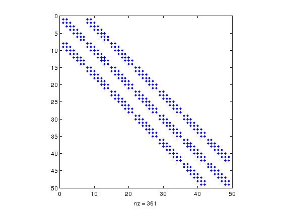
  Figure 5: Structure of diffusion matrix coming from standard MPFA

3.2 Discretization of the convection term

In this section, the convection term

$$\int_{\mathcal{C}_{ij}}\nabla(f\mathcal{U})d\mathcal{C}$$

with

$$f=\left(\begin{array}[]{c}(r-\sigma_{1}^{2}-\frac{1}{2}\rho\sigma_{1}\sigma_{2})x\\ \\ (r-\sigma_{2}^{2}-\frac{1}{2}\rho\sigma_{1}\sigma_{2})y\end{array}\right)=\left(\begin{array}[]{c}p\\ \\ q\end{array}\right)$$

will be approximated by the upwind methods (first and second order).

3.2.1 First order upwind

The first order upwind method discussed by [LeVeque, 2004, chapter 4.8] or Tambue [2016] will be applied to approximate the second term of (20). Using the divergence theorem, we have for $i,j=2,...,N$

$$I^{ij}=\int_{\mathcal{C}_{ij}}\nabla(f\mathcal{U})d\mathcal{C}=\int_{\partial\mathcal{C}_{ij}}(f\cdot\mathcal{U})\cdot\vec{n}d\partial\mathcal{C}.$$ (65)

Note that $I^{ij}$ is calculated by summing up the flux through the edges of the control volume $\mathcal{C}_{ij}$. The flux through an edge using the first order upwind will depend on the sign of $f\cdot\vec{n}$ on this edge. If the sign of $f\cdot\vec{n}$ is positive, $\mathcal{U}_{ij}$ will be used to approximate $\mathcal{U}$ in the expression $(f\cdot\vec{n}\mathcal{U})$ otherwise we will use the value of $\mathcal{U}$ in other side of the edge. Note that an edge may be the interface of two control volumes. By doing so, we have for $i,j=1,...,N$

$$I^{ij} = \epsilon_{ij}\mathcal{U}_{i-1,j}+\mu_{ij}\mathcal{U}_{i,j-1}+\Omega_{ij}\mathcal{U}_{ij}+\phi_{ij}\mathcal{U}_{i,j+1}+\Psi_{ij}\mathcal{U}_{i+1,j}.$$ (66)

where

$$\epsilon_{ij}=-l_{j}f_{x}^{i-1}\max(f_{x}^{i-1},0);\leavevmode\nobreak\ \leavevmode\nobreak\ \leavevmode\nobreak\ \leavevmode\nobreak\ \leavevmode\nobreak\ \mu_{ij}=-h_{i}f_{y}^{j-1}\max(f_{y}^{j-1},0)$$

$$\Omega_{ij}=l_{j}\Bigg{(}f_{x}^{i}\max(f_{x}^{i},0)-f_{x}^{i-1}\min(f_{x}^{i-1},0)\Bigg{)}+h_{i}\Bigg{(}f_{y}^{j}\max(f_{y}^{j},0)-f_{y}^{j-1}\min(f_{y}^{j-1},0)\Bigg{)}$$

$$\phi_{ij}=h_{i}f_{y}^{j}\min(f_{y}^{j},0);\leavevmode\nobreak\ \leavevmode\nobreak\ \leavevmode\nobreak\ \leavevmode\nobreak\ \leavevmode\nobreak\ \leavevmode\nobreak\ \leavevmode\nobreak\ \leavevmode\nobreak\ \Psi_{ij}=l_{j}f_{x}^{i}\min(f_{x}^{i},0).$$

with

$$f_{x}^{i}=(r-\sigma_{1}-\frac{1}{2}\rho\sigma_{1}\sigma_{2})x_{i+1}\leavevmode\nobreak\ \leavevmode\nobreak\ \leavevmode\nobreak\ \leavevmode\nobreak\ \leavevmode\nobreak\ \leavevmode\nobreak\ \leavevmode\nobreak\ \leavevmode\nobreak\ \leavevmode\nobreak\ \leavevmode\nobreak\ \leavevmode\nobreak\ \leavevmode\nobreak\ \leavevmode\nobreak\ \leavevmode\nobreak\ \leavevmode\nobreak\ \leavevmode\nobreak\ f_{y}^{j}=(r-\sigma_{2}-\frac{1}{2}\rho\sigma_{1}\sigma_{2})x_{j+1}$$

Let us notice that for the control volumes near to the boundary of the our domain, some terms from the boundary conditions will be involved in (66). Hence, (66) gives

$$I=A_{up}\mathcal{U}+F_{up}$$ (67)

where $A_{up}$ is a $N^{2}\times N^{2}$ matrix

$$I=\begin{bmatrix}I^{11}\\ I^{12}\\ \vdots\\ I^{1N}\\ I^{21}\\ I^{22}\\ \vdots\\ \vdots\\ I^{NN}\\ \end{bmatrix},\leavevmode\nobreak\ \leavevmode\nobreak\ \leavevmode\nobreak\ \leavevmode\nobreak\ \leavevmode\nobreak\ \leavevmode\nobreak\ \mathcal{U}=\begin{bmatrix}\mathcal{U}_{11}\\ \mathcal{U}_{12}\\ \vdots\\ \mathcal{U}_{1N}\\ \mathcal{U}_{21}\\ \mathcal{U}_{22}\\ \vdots\\ \vdots\\ \mathcal{U}_{NN}\\ \end{bmatrix},A_{up}=\begin{bmatrix}H_{1}&P_{1}&0_{N}&\ldots&\ldots&\ldots&0_{N}\\ Q_{2}&H_{2}&P_{2}&\ddots&&&\vdots\\ 0_{N}&Q_{3}&H_{3}&P_{3}&\ddots&&\vdots\\ \vdots&\ddots&\ddots&\ddots&\ddots&\ddots&\vdots\\ \vdots&&\ddots&Q_{N-2}&H_{N-2}&P_{N-2}&0_{N}\\ \vdots&&&\ddots&Q_{N-1}&H_{N-1}&P_{N-1}\\ 0_{N}&\dots&\ldots&\ldots&0_{N}&Q_{N}&H_{N}\end{bmatrix}$$

with $0_{N}$ is $N\times N$ null matrix, $H_{i}$ is a tridiagonal matrix, $P_{i},Q_{i}$ are diagonal matrices and $F_{up}$ is a vector coming from the boundary conditions. Therefore, combining the MPFA method (64) and the first order upwind (67), we have

$$\frac{d\mathcal{U}}{d\tau}=A\mathcal{U}+F$$ (68)

with

$$A=L^{-1}\Bigg{(}A_{mp}+A_{up}+A_{L}\Bigg{)}\leavevmode\nobreak\ \leavevmode\nobreak\ \leavevmode\nobreak\ \leavevmode\nobreak\ \leavevmode\nobreak\ \leavevmode\nobreak\ F=L^{-1}\Bigg{(}F_{mp}+F_{up}\Bigg{)}$$

where $A_{L}$ is a diagonal matrix of size $N^{2}\times N^{2}$ coming from the discretisation of (22). The diagonal elements of $A_{L}$ are $A_{ii}=h_{i}l_{i}\lambda$ for $i=1,...,N$ with $\lambda$ given in (15). The matrix $L$ is also a diagonal matrix of size $N^{2}\times N^{2}$ whose diagonal elements are $L_{ii}=h_{i}l_{i}$ for $i=1,\ldots,N$

3.2.2 Upwind second order

We start by applying the mid-quadrature rule as follows.

$$J^{ij}=\int_{\mathcal{C}_{ij}}\nabla(f\mathcal{U})d\mathcal{C} = mes(\mathcal{C}_{ij})\nabla(f\mathcal{U})|_{(x_{i},y_{j})}$$ (69)

$$= (x_{i+\frac{1}{2}}-x_{i-\frac{1}{2}})(y_{j+\frac{1}{2}}-y_{j-\frac{1}{2}})\Bigg{[}p_{i}\frac{\partial\mathcal{U}_{ij}}{\partial x}+q_{j}\frac{\partial\mathcal{U}_{ij}}{\partial y}+\Bigg{(}\frac{\partial p_{i}}{\partial x}+\frac{\partial q_{j}}{\partial y}\Bigg{)}\mathcal{U}_{ij}\Bigg{]}$$

$$= h_{i}l_{j}\Bigg{[}\Bigg{(}p_{i}\frac{\partial\mathcal{U}_{ij}}{\partial x}+q_{j}\frac{\partial\mathcal{U}_{ij}}{\partial y}\Bigg{)}+\omega\mathcal{U}_{ij}\Bigg{]},\;\;\,i,j=1,\ldots,N.$$

where $\leavevmode\nobreak\ \leavevmode\nobreak\ \leavevmode\nobreak\ \leavevmode\nobreak\ \leavevmode\nobreak\ p_{i}=(r-\sigma_{1}^{2}-\frac{1}{2}\rho\sigma_{1}\sigma_{2})x_{i},\leavevmode\nobreak\ \leavevmode\nobreak\ \leavevmode\nobreak\ q_{j}=(r-\sigma_{2}^{2}-\frac{1}{2}\rho\sigma_{1}\sigma_{2})y_{j}$ and $\omega=2r-\sigma_{1}^{2}-\sigma_{2}^{2}-\rho\sigma_{1}\sigma_{2}$. Let us use the second order upwind to approximate the first derivatives in (69) at the point $(x_{i},y_{j})$.

Approximation of the first derivative using a 3 points stencil

Here, we want to express the first derivative $\frac{\partial\mathcal{U}_{ij}}{\partial x}$ in terms of $\mathcal{U}_{i+2,j},\mathcal{U}_{i+1,j}$ and $\mathcal{U}_{ij}$. Set $h=\underset{1\leq i\leq N}{\max}h_{i}$. Let us find $a,b$ and $c$ such that

$$\frac{\partial\mathcal{U}_{ij}}{\partial x}=a\mathcal{U}_{i+2,j}+b\mathcal{U}_{i+1,j}+c\mathcal{U}_{ij}$$ (70)

Thereby, using a $2^{nd}$ order Taylor expansion at the point $(x_{i},y_{j})$ on $\mathcal{U}_{i+2,j}$ and $\mathcal{U}_{i+1,j}$, we have

$$\frac{\partial\mathcal{U}_{ij}}{\partial x} = a\mathcal{U}_{i+2,j}+b\mathcal{U}_{i+1,j}+c\mathcal{U}_{ij}$$

$$= a\Bigg{(}\mathcal{U}_{ij}+(h_{i+1}+h_{i+2})\frac{\partial\mathcal{U}_{ij}}{\partial x}+\frac{1}{2}(h_{i+1}+h_{i+2})^{2}\frac{\partial^{2}\mathcal{U}_{ij}}{\partial x^{2}}+\mathcal{O}(h^{3})\Bigg{)}+b\Bigg{(}\mathcal{U}_{ij}+h_{i+1}\frac{\partial\mathcal{U}_{ij}}{\partial x}+\frac{1}{2}h_{i+1}^{2}\frac{\partial^{2}\mathcal{U}_{ij}}{\partial x^{2}}+\mathcal{O}(h^{3})\Bigg{)}$$

$$+c\mathcal{U}_{ij}.$$

$$\frac{\partial\mathcal{U}_{ij}}{\partial x} = \Big{(}a+b+c\Big{)}\mathcal{U}_{ij}+\Bigg{(}a(h_{i+1}+h_{i+2})+bh_{i+1}\Bigg{)}\frac{\partial\mathcal{U}_{ij}}{\partial x}+\Bigg{(}\frac{1}{2}a\Big{(}h_{i+1}+h_{i+2}\Big{)}^{2}+\frac{1}{2}bh_{i+1}^{2}\Bigg{)}\frac{\partial^{2}\mathcal{U}_{ij}}{\partial x^{2}}+\mathcal{O}(h^{3}).$$

By matching, we have

$$\left\{\begin{array}[]{l}a+b+c=0\\ \\ a(h_{i+1}+h_{i+2})+bh_{i+1}\leavevmode\nobreak\ =1\\ \\ \frac{1}{2}a\Big{(}h_{i+1}+h_{i+2}\Big{)}^{2}+\frac{1}{2}bh_{i+1}^{2}=0\end{array}\right.$$ (76)

Solving (76), we have

$$a=-\frac{h_{i+1}}{h_{i+2}(h_{i+1}+h_{i+2})}\leavevmode\nobreak\ \leavevmode\nobreak\ \leavevmode\nobreak\ \leavevmode\nobreak\ \leavevmode\nobreak\ \leavevmode\nobreak\ \leavevmode\nobreak\ \leavevmode\nobreak\ \leavevmode\nobreak\ \leavevmode\nobreak\ \leavevmode\nobreak\ \leavevmode\nobreak\ \leavevmode\nobreak\ \leavevmode\nobreak\ \leavevmode\nobreak\ \leavevmode\nobreak\ b=\frac{h_{i+1}+h_{i+2}}{h_{i+1}h_{i+2}}\leavevmode\nobreak\ \leavevmode\nobreak\ \leavevmode\nobreak\ \leavevmode\nobreak\ \leavevmode\nobreak\ \leavevmode\nobreak\ \leavevmode\nobreak\ \leavevmode\nobreak\ \leavevmode\nobreak\ \leavevmode\nobreak\ \leavevmode\nobreak\ \leavevmode\nobreak\ \leavevmode\nobreak\ \leavevmode\nobreak\ \leavevmode\nobreak\ c=\frac{h_{i+1}^{2}-\Big{(}h_{i+1}+h_{i+2}\Big{)}^{2}}{h_{i+1}+h_{i+2}}.$$ (77)

Therefore we have

$$\frac{\partial\mathcal{U}_{ij}}{\partial x}\approx\frac{-h_{i+1}^{2}\mathcal{U}_{i+2,j}+(h_{i+1}+h_{i+2})^{2}\mathcal{U}_{i+1,j}+(h_{i+1}^{2}-(h_{i+1}+h_{i+2})^{2})\mathcal{U}_{ij}}{h_{i+1}h_{i+2}(h_{i+1}+h_{i+2})}.\\$$ (78)

Application to the $2^{nd}$ order upwind method on non uniform grids
By analogy with the procedure to get the expression in (78), the term $p_{i}\frac{\partial\mathcal{U}_{ij}}{\partial x}$ is approximated as follows:

• $p_{i}>0$ then

  $$p_{i}\frac{\partial\mathcal{U}_{ij}}{\partial x}\approx p_{i}\frac{(h_{i+1}+h_{i+2})^{2}\mathcal{U}_{i+1,j}+\Big{[}h_{i+1}^{2}-(h_{i+1}+h_{i+2})^{2}\Big{]}\mathcal{U}_{ij}-h_{i+1}^{2}\mathcal{U}_{i+2,j}}{h_{i+1}h_{i+2}(h_{i+1}+h_{i+2})}$$

• $p_{i}<0$ then

  $$p_{i}\frac{\partial\mathcal{U}_{ij}}{\partial x}\approx p_{i}\frac{-(h_{i}+h_{i-1})^{2}\mathcal{U}_{i-1,j}+\Big{[}(h_{i}+h_{i-1})^{2}-h_{i}^{2}\Big{]}\mathcal{U}_{ij}+h_{i}^{2}\mathcal{U}_{i-2,j}}{h_{i}h_{i-1}(h_{i}+h_{i-1})}$$

Similarly for the first derivative $\frac{\partial\mathcal{U}_{ij}}{\partial y}$, we have

• when $q_{j}>0$ then

  $$q_{j}\frac{\partial\mathcal{U}_{ij}}{\partial y}\approx q_{j}\frac{(l_{j+1}+l_{j+2})^{2}\mathcal{U}_{i,j+1}+\Big{[}l_{j+1}^{2}-(l_{j+1}+l_{j+2})^{2}\Big{]}\mathcal{U}_{ij}-l_{j+1}^{2}\mathcal{U}_{i,j+2}}{l_{j+1}l_{j+2}(l_{j+1}+l_{j+2})}$$

• when $q_{j}<0$

  $$q_{j}\frac{\partial\mathcal{U}_{ij}}{\partial y}\approx q_{j}\frac{-(l_{j}+l_{j-1})^{2}\mathcal{U}_{i,j-1}+\Big{[}(l_{j}+l_{j-1})^{2}-l_{j}^{2}\Big{]}\mathcal{U}_{ij}+l_{j}^{2}\mathcal{U}_{i,j-2}}{l_{j}l_{j-1}(l_{j}+l_{j-1})}.$$

By combining $(i),(ii),(iii),(iv)$ in (69), for $i,j=2,\ldots,N-1$, we have

(79)

$$J^{ij} = \epsilon_{ij}\mathcal{U}_{i-2,j}+\eta_{ij}\mathcal{U}_{i-1,j}+\kappa_{ij}\mathcal{U}_{i,j-2}+\mu_{ij}\mathcal{U}_{i,j-1}+\Omega_{ij}\mathcal{U}_{ij}+\phi_{ij}\mathcal{U}_{i,j+1}+\Psi_{ij}\mathcal{U}_{i,j+2}+\Delta_{ij}\mathcal{U}_{i+1,j}+\Pi_{ij}\mathcal{U}_{i+2,j}$$

where

$$\epsilon_{ij}=\frac{h_{i}^{2}}{h_{i}h_{i-1}(h_{i}+h_{i-1})}\min(p_{i},0)\leavevmode\nobreak\ \leavevmode\nobreak\ \leavevmode\nobreak\ \leavevmode\nobreak\ \leavevmode\nobreak\ \leavevmode\nobreak\ \leavevmode\nobreak\ \leavevmode\nobreak\ \leavevmode\nobreak\ \eta_{ij}=-\frac{(h_{i}+h_{i-1})^{2}}{h_{i}h_{i-1}(h_{i}+h_{i-1})}\min(p_{i},0)\leavevmode\nobreak\ \leavevmode\nobreak\ \leavevmode\nobreak\ \leavevmode\nobreak\ \leavevmode\nobreak\ \leavevmode\nobreak\ \leavevmode\nobreak\ \leavevmode\nobreak\ \kappa_{ij}=\frac{l_{j}^{2}}{l_{j}l_{j-1}(l_{j}+l_{j-1})}\min(q_{j},0)$$

$$\leavevmode\nobreak\ \leavevmode\nobreak\ \leavevmode\nobreak\ \leavevmode\nobreak\ \leavevmode\nobreak\ \leavevmode\nobreak\ \leavevmode\nobreak\ \leavevmode\nobreak\ \leavevmode\nobreak\ \mu_{ij}=-\frac{(l_{j}+l_{j-1})^{2}}{l_{j}l_{j-1}(l_{j}+l_{j-1})}\min(q_{j},0)$$

$$\Omega_{ij}=\omega+\frac{(h_{i}+h_{i-1})^{2}-h_{i}^{2}}{h_{i}h_{i-1}(h_{i}+h_{i-1})}\min(p_{i},0)+\frac{h_{i+1}^{2}-(h_{i+1}+h_{i+2})^{2}}{h_{i+1}h_{i+2}(h_{i+1}+h_{i+2})}\max(p_{i},0)+\frac{(l_{j}+l_{j-1})^{2}-l_{j}^{2}}{l_{j}l_{j-1}(l_{j}+l_{j-1})}\min(q_{j},0)$$

$$\leavevmode\nobreak\ \leavevmode\nobreak\ \leavevmode\nobreak\ \leavevmode\nobreak\ \leavevmode\nobreak\ \leavevmode\nobreak\ \leavevmode\nobreak\ +\frac{l_{j+1}^{2}-(l_{j+1}+l_{j+2})^{2}}{l_{j+1}l_{j+2}(l_{j+1}+l_{j+2})}\max(q_{j},0)$$

$$\phi_{ij}=\frac{(l_{j+1}+l_{j+2})^{2}}{l_{j+1}l_{j+2}(l_{j+1}+l_{j+2})}\max(q_{j},0)\leavevmode\nobreak\ \leavevmode\nobreak\ \leavevmode\nobreak\ \leavevmode\nobreak\ \leavevmode\nobreak\ \leavevmode\nobreak\ \leavevmode\nobreak\ \Psi_{ij}=-\frac{l_{j+1}^{2}}{l_{j+1}l_{j+2}(l_{j+1}+l_{j+2})}\max(q_{j},0)\leavevmode\nobreak\ \leavevmode\nobreak\ \leavevmode\nobreak\ \leavevmode\nobreak\ \leavevmode\nobreak\ \leavevmode\nobreak\ \leavevmode\nobreak\$$

$$\Delta_{ij}=\frac{(h_{i+1}+h_{i+2})^{2}}{h_{i+1}h_{i+2}(h_{i+1}+h_{i+2})}\max(p_{i},0)\leavevmode\nobreak\ \leavevmode\nobreak\ \leavevmode\nobreak\ \leavevmode\nobreak\ \leavevmode\nobreak\ \leavevmode\nobreak\ \leavevmode\nobreak\ \leavevmode\nobreak\ \leavevmode\nobreak\ \leavevmode\nobreak\ \Pi_{ij}=-\frac{h_{i+1}^{2}}{h_{i+1}h_{i+2}(h_{i+1}+h_{i+2})}\max(p_{i},0).$$

For the control volumes near the boundary of the study domain, two ghost points or the first order upwind method can be used. Finally, we have the following matrix form

$$J=A_{2up}\mathcal{U}+F_{2up}$$ (80)

where

$$J=\begin{bmatrix}J^{11}\\ J^{12}\\ \vdots\\ J^{1N}\\ J^{21}\\ J^{22}\\ \vdots\\ J^{2N}\\ \vdots\\ \vdots\\ J^{NN}\\ \end{bmatrix},F_{2up}=\begin{bmatrix}F^{11}_{up}\\ F^{12}_{up}\\ \vdots\\ F^{1N}_{up}\\ F^{21}_{up}\\ F^{22}_{up}\\ \vdots\\ F^{2N}_{up}\\ \vdots\\ \vdots\\ F^{NN}_{up}\end{bmatrix},\leavevmode\nobreak\ \leavevmode\nobreak\ \leavevmode\nobreak\ \leavevmode\nobreak\ \leavevmode\nobreak\ \leavevmode\nobreak\ \mathcal{U}=\begin{bmatrix}\mathcal{U}_{11}\\ \mathcal{U}_{12}\\ \vdots\\ \mathcal{U}_{1N}\\ \mathcal{U}_{21}\\ \mathcal{U}_{22}\\ \vdots\\ \mathcal{U}_{2N}\\ \vdots\\ \vdots\\ \mathcal{U}_{NN}\\ \end{bmatrix}$$

and

$$A_{2up}=\begin{bmatrix}H_{1}&P_{1}&0_{N}&0&\ldots&\ldots&\ldots&&0_{N}&0_{N}\\ Q_{2}&H_{2}&P_{2}&R_{2}&0_{N}&&&&&0_{N}\\ W_{3}&Q_{3}&H_{3}&P_{3}&R_{3}&0_{N}&&&&\vdots\\ 0_{N}&W_{4}&Q_{4}&H_{4}&P_{4}&R_{4}&\ddots\\ 0_{N}&0_{N}&\ddots&\ddots&\ddots&\ddots&\ddots&\ddots\\ \vdots&&\ddots&\ddots&\ddots&\ddots&\ddots&\ddots&\ddots\\ \vdots&&&\ddots&\ddots&\ddots&\ddots&\ddots&\ddots&0_{N}\\ &&&&\ddots&W_{N-2}&Q_{N-2}&H_{N-2}&P_{N-2}&R_{N-2}\\ \vdots&&&&&\ddots&W_{N-1}&Q_{N-1}&H_{N-1}&P_{i,N-1}\\ 0_{N}&\dots&\ldots&\ldots&&\ldots&0_{N}&0_{N}&Q_{N}&H_{N}\\ \end{bmatrix}$$

where $H_{1},H_{N}$ are tridiagonal matrices, for $i=2,\ldots,N-1,\leavevmode\nobreak\ H_{i}$ are penta-diagonal matrices and $P_{i},R_{i},W_{i},Q_{i}$ are diagonal matrices, and $F_{up}$ is a vector coming from the boundary conditions. A structure of the advection matrix using the second order upwind method can be viewed in Figure 6.

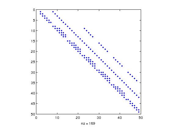
Figure 6: A structure of the advection matrix using 2nd order upwind method.

As for the first order upwinding, combining the MPFA method (64) and the second order upwind method (80), we have

$$\frac{d\mathcal{U}}{d\tau}=A\mathcal{U}+F$$ (81)

$$A=L^{-1}\Bigg{(}A_{mp}+A_{2up}+A_{L}\Bigg{)}\leavevmode\nobreak\ \leavevmode\nobreak\ \leavevmode\nobreak\ \leavevmode\nobreak\ \leavevmode\nobreak\ \leavevmode\nobreak\ F=L^{-1}\Bigg{(}F_{mp}+F_{2up}\Bigg{)},$$

where $A_{L}$ is a diagonal matrix of size $N^{2}\times N^{2}$ coming from the discretisation of (22). The elements of $A_{L}$ are $h_{i}l_{j}\lambda$ for $i,j=1,...,N$ with $\lambda$ given in (15). The matrix $L$ is also a diagonal matrix of size $N^{2}\times N^{2}$ whose diagonal elements are $L_{ii}=h_{i}l_{i}$ for $i=1,\ldots,N$

Actually, the PDE (8) is degenerated when the stock price is approaching zero $(x\rightarrow 0,y\rightarrow 0)$ which has an adverse impact on the accuracy of the numerical method. However, to overcome the degeneracy, we are going to apply a fitted finite volume method in the degeneracy region $(x\rightarrow 0,y\rightarrow 0)$. More details about this fitted method is given in the next section.

3.3 Fitted Multi-Point Flux Approximation

The fitted Multi-Point Flux Approximation is a combination of the fitted finite volume method ( see Huang et al. [2006, 2009]) and the Multi-Point Flux Approximation method. The fitted finite volume helps to deal with the degeneracy of the PDE (8). We approximate simultaneously the diffusion term and the convection term in the degeneracy region by solving a two-points boundary problem. In the region where the PDE is not degenerated, we apply the standard Multi-point flux approximation to the diffusion term as described in the previous section.
Let us set

$$k(\mathcal{U})=\nabla\cdot(\mathbf{M}\nabla\mathcal{U}+f\mathcal{U})$$ (82)

where $\mathbf{M}$ and $f$ are defined in (15). Thereby, we have the following decomposition over a control volume $\mathcal{C}_{ij}$, for $\leavevmode\nobreak\ \leavevmode\nobreak\ i,j=1,...,N$

$$\int_{\mathcal{C}_{ij}}\nabla k(\mathcal{U})d\mathcal{C} = \int_{\mathcal{C}_{ij}}\nabla\cdot(M\nabla\mathcal{U}+f\mathcal{U})d\mathcal{C}$$

$$= \int_{\partial\mathcal{C}_{ij}}(M\nabla\mathcal{U}+f\mathcal{U})\cdot\vec{n}d\partial\mathcal{C}$$

$$= \int_{(x_{i+\frac{1}{2}},y_{j-\frac{1}{2}})}^{(x_{i+\frac{1}{2}},y_{j+\frac{1}{2}})}\Bigg{(}m_{11}\frac{\partial\mathcal{U}}{\partial x}+m_{12}\frac{\partial\mathcal{U}}{\partial y}+p\mathcal{U}\Bigg{)}dy$$

$$-\int_{(x_{i-\frac{1}{2}},y_{j-\frac{1}{2}})}^{(x_{i-\frac{1}{2}},y_{j+\frac{1}{2}})}\Bigg{(}m_{11}\frac{\partial\mathcal{U}}{\partial x}+m_{12}\frac{\partial\mathcal{U}}{\partial y}+p\mathcal{U}\Bigg{)}dy$$

$$+\int_{(x_{i-\frac{1}{2}},y_{j+\frac{1}{2}})}^{(x_{i+\frac{1}{2}},y_{j+\frac{1}{2}})}\Bigg{(}m_{21}\frac{\partial\mathcal{U}}{\partial x}+m_{22}\frac{\partial\mathcal{U}}{\partial y}+q\mathcal{U}\Bigg{)}dx$$

$$-\int_{(x_{i-\frac{1}{2}},y_{j-\frac{1}{2}})}^{(x_{i+\frac{1}{2}},y_{j-\frac{1}{2}})}\Bigg{(}m_{21}\frac{\partial\mathcal{U}}{\partial x}+m_{22}\frac{\partial\mathcal{U}}{\partial y}+q\mathcal{U}\Bigg{)}dx$$

with $\vec{n}$ is the outward unit normal vector, $m_{11},m_{12},m_{21},m_{22}$ the coefficients of the matrix $\mathbf{M}$ and $p,q$ coefficients of vector $f$ defined in (15).
In their work, Huang et al. [2006, 2009] showed how the fitted finite method is used to approximate each of the integral in (3.3).

3.3.1 Fitted Finite volume method in the degeneracy region

Following Huang et al. [2006], the fitted finite volume method is used to approximate the flux through the edges which are effectively in the degeneracy region notably the western edge of the control volume $\mathcal{C}_{1,j}$ for $j=1,\ldots,N$ and the southern edge of the control volume $\mathcal{C}_{i,1}$ for $i=1,\ldots,N$ .
Thereby, the flux through the southern edge of the control volume $\mathcal{C}_{i,1}$ for $i=1,\ldots,N$ is calculated as follows.

Figure 7:

The fitted finite volume method is applied to approximate the integral along the southern edge of control volume $\mathcal{C}_{i,1}$. The idea is to approximate the integral over $[x_{i-\frac{1}{2}};x_{i+\frac{1}{2}}]$ by a constant. We start by applying the mid-quadrature rule as follows:

$$\int_{(x_{i-\frac{1}{2}},y_{\frac{1}{2}})}^{(x_{i+\frac{1}{2}},y_{\frac{1}{2}})}\Bigg{(}m_{21}\frac{\partial\mathcal{U}}{\partial x}+m_{22}\frac{\partial\mathcal{U}}{\partial y}+q\mathcal{U}\Bigg{)}dx\approx\Bigg{(}m_{21}\frac{\partial\mathcal{U}}{\partial x}+m_{22}\frac{\partial\mathcal{U}}{\partial y}+q\mathcal{U}\Bigg{)}_{|_{x_{i},y_{\frac{1}{2}}}}\cdot h_{i}$$ (84)

Besides we have

$$m_{21}\frac{\partial\mathcal{U}}{\partial x}+m_{22}\frac{\partial\mathcal{U}}{\partial y}+q\mathcal{U}=y\Bigg{(}ey\frac{\partial\mathcal{U}}{\partial y}+h^{\prime}\frac{\partial\mathcal{U}}{\partial x}+k\mathcal{U}\Bigg{)}$$ (85)

with $e=\frac{1}{2}\sigma_{2}^{2},\leavevmode\nobreak\ \leavevmode\nobreak\ \leavevmode\nobreak\ k=r-\sigma_{2}^{2}-\frac{1}{2}\rho\sigma_{1}\sigma_{2}$ and $h^{\prime}=\frac{1}{2}\rho\sigma_{1}\sigma_{2}x$.

We want to approximate

$$f(\mathcal{U})=ey\frac{\partial\mathcal{U}}{\partial y}+k\mathcal{U}$$

by a linear function over $I_{y_{1}}=(0,y_{1})$ satisfying the following two-points boundary value problem

$$\left\{\begin{array}[]{l}f^{\prime}(\mathcal{U})\leavevmode\nobreak\ \leavevmode\nobreak\ \leavevmode\nobreak\ \leavevmode\nobreak\ =\Bigg{(}ey\frac{\partial\mathcal{U}}{\partial y}+k\mathcal{U}\Bigg{)}^{\prime}=K_{1}\\ \\ \mathcal{U}(x_{i},0)=\mathcal{U}_{i,0}\leavevmode\nobreak\ \leavevmode\nobreak\ \leavevmode\nobreak\ \leavevmode\nobreak\ \leavevmode\nobreak\ \leavevmode\nobreak\ \leavevmode\nobreak\ \leavevmode\nobreak\ \leavevmode\nobreak\ \mathcal{U}(x_{i},y_{1})=\mathcal{U}_{i,1}\end{array}\right.$$ (89)

By solving this problem we get

$$\mathcal{U}=\mathcal{U}_{i,0}+(\mathcal{U}_{i,1}-\mathcal{U}_{i,0})\frac{y}{y_{1}}$$ (90)

Thereby, by using (84), (89), (90) and the forward difference for approximating the first partial derivative $\frac{\partial\mathcal{U}}{\partial x}$ we get

$$\int_{(x_{i-\frac{1}{2}},y_{\frac{1}{2}})}^{(x_{i+\frac{1}{2}},y_{\frac{1}{2}})}\Bigg{(}m_{21}\frac{\partial\mathcal{U}}{\partial x}+m_{22}\frac{\partial\mathcal{U}}{\partial y}+q\mathcal{U}\Bigg{)}dx\approx\frac{1}{2}y_{1}\Big{[}\frac{1}{2}h_{i}(e+k)-h_{i}^{\prime}\Big{]}\mathcal{U}_{i,1}+\frac{1}{2}h_{i}^{\prime}y_{1}\mathcal{U}_{i+1,1}-\frac{1}{4}y_{1}h_{i}(e-k)\mathcal{U}_{i,0}$$ (91)

where

$$e=\frac{1}{2}\sigma_{2}^{2},\leavevmode\nobreak\ \leavevmode\nobreak\ \leavevmode\nobreak\ \leavevmode\nobreak\ \leavevmode\nobreak\ \leavevmode\nobreak\ \leavevmode\nobreak\ \leavevmode\nobreak\ \leavevmode\nobreak\ k=r-\sigma_{2}^{2}-\frac{1}{2}\rho\sigma_{1}\sigma_{2}\leavevmode\nobreak\ \leavevmode\nobreak\ \leavevmode\nobreak\ \leavevmode\nobreak\ \leavevmode\nobreak\ \leavevmode\nobreak\ \leavevmode\nobreak\ h_{i}^{\prime}=\frac{1}{2}\rho\sigma_{1}\sigma_{2}x_{i}\leavevmode\nobreak\ \leavevmode\nobreak\ \leavevmode\nobreak\ \leavevmode\nobreak\ \leavevmode\nobreak\ \leavevmode\nobreak\ h_{i}=x_{i+\frac{1}{2}}-x_{i-\frac{1}{2}}$$

Similarly, for the western edge of the control volume $\mathcal{C}_{1,j},\leavevmode\nobreak\ \leavevmode\nobreak\ for\leavevmode\nobreak\ \leavevmode\nobreak\ j=1,...,N$, we have

$$\int_{(x_{\frac{1}{2}},y_{j-\frac{1}{2}})}^{(x_{\frac{1}{2}},y_{j+\frac{1}{2}})}\Bigg{(}m_{11}\frac{\partial\mathcal{U}}{\partial x}+m_{12}\frac{\partial\mathcal{U}}{\partial y}+p\mathcal{U}\Bigg{)}dy\approx\frac{1}{2}x_{1}\Big{[}\frac{1}{2}l_{j}(a+b)-d_{j}\Big{]}\mathcal{U}_{1,j}+\frac{1}{2}d_{j}x_{1}\mathcal{U}_{1,j+1}-\frac{1}{4}l_{j}x_{1}(a-b)\mathcal{U}_{0,j}$$ (92)

with

$$a=\frac{1}{2}\sigma_{1}^{2}\leavevmode\nobreak\ \leavevmode\nobreak\ \leavevmode\nobreak\ \leavevmode\nobreak\ \leavevmode\nobreak\ \leavevmode\nobreak\ \leavevmode\nobreak\ \leavevmode\nobreak\ \leavevmode\nobreak\ b=r-\sigma_{1}^{2}-\frac{1}{2}\rho\sigma_{1}\sigma_{2}\leavevmode\nobreak\ \leavevmode\nobreak\ \leavevmode\nobreak\ \leavevmode\nobreak\ \leavevmode\nobreak\ \leavevmode\nobreak\ \leavevmode\nobreak\ \leavevmode\nobreak\ \leavevmode\nobreak\ d_{j}=\frac{1}{2}\rho\sigma_{1}\sigma_{2}y_{j}\leavevmode\nobreak\ \leavevmode\nobreak\ \leavevmode\nobreak\ \leavevmode\nobreak\ \leavevmode\nobreak\ \leavevmode\nobreak\ \leavevmode\nobreak\ \leavevmode\nobreak\ l_{j}=y_{j+\frac{1}{2}}-y_{j-\frac{1}{2}}$$

3.3.2 Fitted Multi-Point Flux Approximation

The fitted Multi-Point Approximation method consists of calculating the flux through the edges which are totally in the degeneracy region using the fitted finite volume method as described in the previous paragraph. For the edges which are not totally in the degeneracy region, the flux is approximated using simultaneously the Multi-point flux approximation and the upwind methods (first order or second order). In the other hand, the MPFA method and the upwind methods are used to approximate respectively the diffusion term and the convection term over the control volumes which are not in the degeneracy region.
Considering (3.3), in fact, in the control volume $\mathcal{C}_{11}$, the southern and western edges are in the degeneracy region, the northern and the eastern edges are not in the degeneracy region. Thereby, the flux through the southern and western edges are approximated using the fitted finite volume method, while the flux through the eastern and northern edges are approximated using simultaneously of the MPFA method and the upwind method. This gives

$$\int_{{\mathcal{C}}_{11}}\nabla k(\mathcal{U}) \approx a_{11}^{1}\mathcal{U}_{11}+b_{11}^{1}\mathcal{U}_{21}+c_{11}^{1}\mathcal{U}_{22}+d_{11}^{1}\mathcal{U}_{12}+\omega_{11}^{1}\mathcal{U}_{02}+\phi_{11}^{1}\mathcal{U}_{01}$$ (93)

$$+r_{11}^{1}\mathcal{U}_{10}+s_{11}^{1}\mathcal{U}_{20}$$

with

$$a_{11}^{1}=T_{11}^{22}+T_{23}^{21}+T_{31}^{22}+T_{42}^{12}+l_{1}\max(f_{x}^{2},0)+h_{1}\max(f_{y}^{2},0)-\frac{1}{2}x_{1}\Big{[}\frac{1}{2}l_{1}(a+b)-d_{1}\Big{]}$$

$$\leavevmode\nobreak\ \leavevmode\nobreak\ \leavevmode\nobreak\ \leavevmode\nobreak\ \leavevmode\nobreak\ \leavevmode\nobreak\ \leavevmode\nobreak\ \leavevmode\nobreak\ \leavevmode\nobreak\ -\frac{1}{2}y_{1}\Big{[}\frac{1}{2}h_{1}(e+k)-h_{1}^{\prime}\Big{]}$$

$$b_{11}^{1}=T_{12}^{22}+T_{24}^{21}+T_{32}^{22}+l_{1}\min(f_{x}^{2},0)-\frac{1}{2}h_{1}^{\prime}y_{1};\leavevmode\nobreak\ \leavevmode\nobreak\ \leavevmode\nobreak\ \leavevmode\nobreak\ \leavevmode\nobreak\ \leavevmode\nobreak\ \leavevmode\nobreak\ \leavevmode\nobreak\ c^{1}_{11}=T_{14}^{22}+T_{34}^{22}$$

$$d_{11}^{1}=T_{13}^{22}+T_{33}^{22}+T_{44}^{12}+h_{1}\min(f_{y}^{2},0)-\frac{1}{2}d_{1}x_{1};\leavevmode\nobreak\ \leavevmode\nobreak\ \leavevmode\nobreak\ \leavevmode\nobreak\ \leavevmode\nobreak\ \leavevmode\nobreak\ \leavevmode\nobreak\ \leavevmode\nobreak\ \omega_{11}^{1}=T_{43}^{12}\leavevmode\nobreak\ \leavevmode\nobreak\ \leavevmode\nobreak\ \leavevmode\nobreak\ \leavevmode\nobreak\ \leavevmode\nobreak\ \leavevmode\nobreak\ \leavevmode\nobreak\ \leavevmode\nobreak\ \leavevmode\nobreak\ \leavevmode\nobreak\$$

$$\phi_{11}^{1}=T_{41}^{12}+\frac{1}{4}l_{1}x_{1}(a-b)\leavevmode\nobreak\ \leavevmode\nobreak\ \leavevmode\nobreak\ \leavevmode\nobreak\ \leavevmode\nobreak\ \leavevmode\nobreak\ \leavevmode\nobreak\ \leavevmode\nobreak\ \leavevmode\nobreak\ \leavevmode\nobreak\ \leavevmode\nobreak\ r_{11}^{1}=T_{21}^{21}+\frac{1}{4}h_{1}y_{1}(e-k)\leavevmode\nobreak\ \leavevmode\nobreak\ \leavevmode\nobreak\ \leavevmode\nobreak\ \leavevmode\nobreak\ \leavevmode\nobreak\ \leavevmode\nobreak\ s_{11}^{1}=T_{22}^{21}$$

Similarly, for the control volume $\mathcal{C}_{1,j}\leavevmode\nobreak\ \leavevmode\nobreak\ \leavevmode\nobreak\ \leavevmode\nobreak\ j=1,\ldots,N$, we have

$$\int_{{\mathcal{C}}_{1,j}}\nabla k(\mathcal{U}) \approx a_{1,j}^{1}\mathcal{U}_{1,j}+bb_{1,j}\mathcal{U}_{2,j}+c_{1,j}^{1}\mathcal{U}_{2,j+1}+d_{1,j}^{1}\mathcal{U}_{1,j+1}+\gamma_{1,j}^{1}\mathcal{U}_{1,j-1}+\lambda_{1,j}^{1}\mathcal{U}_{2,j-1}$$ (94)

$$\omega_{1,j}^{1}\mathcal{U}_{0,j+1}+\phi_{1,j}^{1}\mathcal{U}_{0,j}+\Upsilon_{1,j}^{1}\mathcal{U}_{0,j-1}$$

$$a_{1,j}^{1}=T_{11}^{2,j+1}+T_{23}^{2,j}+T_{31}^{2,j+1}+T_{42}^{1,j+1}-T_{33}^{2,j}-T_{44}^{1,j}-\frac{1}{2}x_{1}\Big{(}\frac{1}{2}l_{j}(a+b)-d_{j}\Big{)}$$

$$\leavevmode\nobreak\ \leavevmode\nobreak\ \leavevmode\nobreak\ \leavevmode\nobreak\ \leavevmode\nobreak\ \leavevmode\nobreak\ \leavevmode\nobreak\ \leavevmode\nobreak\ \leavevmode\nobreak\ +l_{j}\max(f_{x}^{2},0)+h_{1}\max(f^{j+1}_{y},0)-h_{1}\min(f^{j}_{y},0)$$

$$b_{1,j}^{1}=T_{12}^{2,j+1}+T_{24}^{2,j}+T_{32}^{2,j+1}-T_{34}^{2,j}+l_{j}\min(f_{x}^{2},0);\leavevmode\nobreak\ \leavevmode\nobreak\ \leavevmode\nobreak\ \leavevmode\nobreak\ \leavevmode\nobreak\ \leavevmode\nobreak\ \leavevmode\nobreak\ \leavevmode\nobreak\ \leavevmode\nobreak\ \leavevmode\nobreak\ \leavevmode\nobreak\ \leavevmode\nobreak\ c_{1,j}^{1}=T_{14}^{2,j+1}+T_{34}^{2,j+1};$$

$$d_{1,j}^{1}=T_{13}^{2,j+1}+T_{33}^{2,j+1}+T_{44}^{1,j+1}+h_{1}\min(f_{y}^{j+1},0)-\frac{1}{2}d_{j}x_{1}+$$

$$\gamma_{1,j}^{1}=T_{21}^{2,j}-T_{31}^{2,j}-T_{42}^{1,j}-h_{1}\max(f_{y}^{j},0);\leavevmode\nobreak\ \leavevmode\nobreak\ \leavevmode\nobreak\ \leavevmode\nobreak\ \leavevmode\nobreak\ \leavevmode\nobreak\ \leavevmode\nobreak\ \leavevmode\nobreak\ \leavevmode\nobreak\ \leavevmode\nobreak\ \leavevmode\nobreak\ \leavevmode\nobreak\ \leavevmode\nobreak\ \lambda_{1,j}^{1}=T_{22}^{2,j}-T_{32}^{2,j};$$

$$\omega_{1,j}^{1}=T_{43}^{1,j+1};\leavevmode\nobreak\ \leavevmode\nobreak\ \leavevmode\nobreak\ \leavevmode\nobreak\ \leavevmode\nobreak\ \leavevmode\nobreak\ \leavevmode\nobreak\ \leavevmode\nobreak\ \leavevmode\nobreak\ \leavevmode\nobreak\ \leavevmode\nobreak\ \leavevmode\nobreak\ \leavevmode\nobreak\ \leavevmode\nobreak\ \phi_{1,j}^{1}=T_{41}^{1,j+1}-T_{43}^{1,j}+\frac{1}{4}l_{j}x_{1}(a-b);\leavevmode\nobreak\ \leavevmode\nobreak\ \leavevmode\nobreak\ \leavevmode\nobreak\ \leavevmode\nobreak\ \leavevmode\nobreak\ \leavevmode\nobreak\ \leavevmode\nobreak\ \Upsilon_{1,j}^{1}=-T_{41}^{1,j};$$

For the control $\mathcal{C}_{i,1}\leavevmode\nobreak\ \leavevmode\nobreak\ \leavevmode\nobreak\ \leavevmode\nobreak\ i=2,\ldots,N$, we have:

$$\int_{{\mathcal{C}}_{i,1}}\nabla k(\mathcal{U}) \approx a_{i,1}^{1}\mathcal{U}_{i,1}+b_{i,1}^{1}\mathcal{U}_{i+1,1}+c_{i,1}^{1}\mathcal{U}_{i+1,2}+d_{i,1}^{1}\mathcal{U}_{i,2}+e_{i,1}^{1}\mathcal{U}_{i-1,2}+\alpha_{i,1}^{1}\mathcal{U}_{i-1,1}+t_{i,1}^{1}\mathcal{U}_{i-1,0}$$ (95)

$$+r_{i,1}^{1}\mathcal{U}_{i,0}+s_{i,1}^{1}\mathcal{U}_{i+1,0}$$

with

$$a_{i,1}^{1}=T_{11}^{i+1,2}+T_{23}^{i+1,1}+T_{31}^{i+1,2}+T_{42}^{i,2}-T_{12}^{i,2}-T_{24}^{i,1}-\frac{1}{2}y_{1}\Big{[}\frac{1}{2}h_{i}(e+k)-h_{i}^{\prime}\Big{]}$$

$$\leavevmode\nobreak\ \leavevmode\nobreak\ \leavevmode\nobreak\ \leavevmode\nobreak\ \leavevmode\nobreak\ \leavevmode\nobreak\ \leavevmode\nobreak\ \leavevmode\nobreak\ \leavevmode\nobreak\ \leavevmode\nobreak\ \leavevmode\nobreak\ +l_{1}\max(f_{x}^{i+1},0)+h_{i}\max(f_{y}^{2},0)\Big{)}-l_{1}\min(f_{x}^{i},0)$$

$$b_{i,1}^{1}=T_{12}^{i+1,2}+T_{24}^{i+1,1}+T_{32}^{i+1,2}+l_{i}\min(f_{x}^{i+1},0)-\frac{1}{2}h_{i}^{\prime}y_{1};\leavevmode\nobreak\ \leavevmode\nobreak\ \leavevmode\nobreak\ \leavevmode\nobreak\ \leavevmode\nobreak\ \leavevmode\nobreak\ \leavevmode\nobreak\ \leavevmode\nobreak\ \leavevmode\nobreak\ \leavevmode\nobreak\ \leavevmode\nobreak\ \leavevmode\nobreak\ \leavevmode\nobreak\ \leavevmode\nobreak\ \leavevmode\nobreak\ c_{i,1}^{1}=T_{14}^{i+1,2}+T_{34}^{i+1,2}$$

$$d_{i,1}^{1}=T_{13}^{i+1,2}+T_{33}^{i+1,2}+T_{44}^{i,2}-T_{14}^{i,2}+h_{i}\min(f_{y}^{2},0);\leavevmode\nobreak\ \leavevmode\nobreak\ \leavevmode\nobreak\ \leavevmode\nobreak\ \leavevmode\nobreak\ \leavevmode\nobreak\ \leavevmode\nobreak\ \leavevmode\nobreak\ \leavevmode\nobreak\ \leavevmode\nobreak\ \leavevmode\nobreak\ \leavevmode\nobreak\ \leavevmode\nobreak\ \leavevmode\nobreak\ \leavevmode\nobreak\ \leavevmode\nobreak\ \leavevmode\nobreak\ \leavevmode\nobreak\ \leavevmode\nobreak\ \leavevmode\nobreak\ \leavevmode\nobreak\ \leavevmode\nobreak\ e_{i,1}^{1}=T_{43}^{i,2}-T_{13}^{i,2}$$

$$\alpha_{i,1}^{1}=T_{41}^{i,2}-T_{11}^{i,2}-T_{23}^{i,1}-l_{1}\max(f_{x}^{i},0);\leavevmode\nobreak\ \leavevmode\nobreak\ \leavevmode\nobreak\ \leavevmode\nobreak\ \leavevmode\nobreak\ \leavevmode\nobreak\ \leavevmode\nobreak\ \leavevmode\nobreak\ \leavevmode\nobreak\ \leavevmode\nobreak\ \leavevmode\nobreak\ t_{i,1}^{1}=-T_{21}^{i,1};$$

$$r_{i,1}^{1}=T_{21}^{i+1,1}-T_{22}^{i,1}+\frac{1}{4}y_{1}h_{i}(e-k)\leavevmode\nobreak\ \leavevmode\nobreak\ \leavevmode\nobreak\ \leavevmode\nobreak\ \leavevmode\nobreak\ \leavevmode\nobreak\ \leavevmode\nobreak\ \leavevmode\nobreak\ s_{i,1}^{1}=T_{22}^{i+1,1}$$

As we already mentioned, for the control volumes which are not in the degeneracy region, we use the multi-Point flux approximation to approximate the diffusion term and the upwind methods (first and second order) to approximate the convection term. So by combining as before, we obtain the following ODE

$$\frac{d\mathcal{U}}{d\tau}=A\mathcal{U}+F$$ (96)

where

$$\mathcal{U}=\begin{bmatrix}\mathcal{U}_{11}\\ \mathcal{U}_{12}\\ \vdots\\ \mathcal{U}_{1N}\\ \mathcal{U}_{21}\\ \mathcal{U}_{22}\\ \vdots\\ \mathcal{U}_{2N}\\ \vdots\\ \vdots\\ \mathcal{U}_{N,1}\\ \mathcal{U}_{N,2}\\ \vdots\\ \mathcal{U}_{NN}\end{bmatrix}\leavevmode\nobreak\ \leavevmode\nobreak\ \leavevmode\nobreak\ \leavevmode\nobreak\ A=L^{-1}\Big{(}Z+A_{L}\Big{)}\leavevmode\nobreak\ \leavevmode\nobreak\$$

with $F$ the vector of boundary conditions, $A_{L}$ is a diagonal matrix of size $N^{2}\times N^{2}$ coming from the discretisation of (22). The elements of $A_{L}$ are $h_{i}l_{j}\lambda$ for $i,j=1,...,N$ with $\lambda$ given in (15). The matrix $L$ is also a diagonal matrix of size $N^{2}\times N^{2}$ whose diagonal elements are $h_{i}l_{j}$ for $i,j=1,\ldots,N$ and

$$Z=\begin{bmatrix}D_{1}&K_{1}&0_{N}&\ldots&\ldots&\ldots&\ldots&0_{N}\\ L_{2}&D_{2}&K_{2}&\ddots&&&&\vdots\\ 0_{N}&L_{3}&D_{3}&K_{3}&\ddots&&&\vdots\\ \vdots&\ddots&L_{4}&D_{4}&K_{4}&\ddots&&\vdots\\ \vdots&&\ddots&\ddots&\ddots&\ddots&\ddots&\vdots\\ \vdots&&&\ddots&\ddots&\ddots&\ddots&0_{N}&\\ \vdots&&&&\ddots&L_{N-1}&D_{N-1}&K_{N-1}\\ 0_{N}&\ldots&\ldots&\ldots&\ldots&0_{N}&L_{N}&D_{N}\end{bmatrix}$$

The fitted matrix $Z$ uses the first order upwind method. The matrices $D_{i},K_{i},L_{i}$ are tri-diagonal matrices defined as follows. For $i=1,N$

$$k=1,\ldots,N\leavevmode\nobreak\ \leavevmode\nobreak\ (D_{i})_{kk}=a_{1,k}^{1}\leavevmode\nobreak\ \leavevmode\nobreak\ \leavevmode\nobreak\ \leavevmode\nobreak\ \leavevmode\nobreak\ \leavevmode\nobreak\ \leavevmode\nobreak\ \leavevmode\nobreak\ \leavevmode\nobreak\ k=1,\ldots,N-1\leavevmode\nobreak\ \leavevmode\nobreak\ (D_{i})_{k,k+1}=d_{1,k}^{1},\leavevmode\nobreak\ \leavevmode\nobreak\ \leavevmode\nobreak\ \leavevmode\nobreak\ \leavevmode\nobreak\ \leavevmode\nobreak\ \leavevmode\nobreak\ \leavevmode\nobreak\ \leavevmode\nobreak\ \leavevmode\nobreak\ \leavevmode\nobreak\ \leavevmode\nobreak\ k=2,\ldots,N\leavevmode\nobreak\ \leavevmode\nobreak\ (D_{i})_{k,k-1}=\gamma_{1,k}^{1}$$

$$k=1,\ldots,N\leavevmode\nobreak\ \leavevmode\nobreak\ (K_{1})_{kk}=b_{1,k}^{1}\leavevmode\nobreak\ \leavevmode\nobreak\ \leavevmode\nobreak\ \leavevmode\nobreak\ \leavevmode\nobreak\ \leavevmode\nobreak\ \leavevmode\nobreak\ \leavevmode\nobreak\ \leavevmode\nobreak\ k=1,\ldots,N-1\leavevmode\nobreak\ \leavevmode\nobreak\ (K_{1})_{k,k+1}=c_{1,k}^{1},\leavevmode\nobreak\ \leavevmode\nobreak\ \leavevmode\nobreak\ \leavevmode\nobreak\ \leavevmode\nobreak\ \leavevmode\nobreak\ \leavevmode\nobreak\ \leavevmode\nobreak\ \leavevmode\nobreak\ \leavevmode\nobreak\ \leavevmode\nobreak\ \leavevmode\nobreak\ k=2,\ldots,N\leavevmode\nobreak\ \leavevmode\nobreak\ (K_{1})_{k,k-1}=\lambda_{1,k}^{1}$$

$$(L_{N})_{11}=\alpha_{N,1}^{1}\leavevmode\nobreak\ \leavevmode\nobreak\ \leavevmode\nobreak\ (L_{N})_{12}=e_{N,1}^{1}\leavevmode\nobreak\ \leavevmode\nobreak\ \leavevmode\nobreak\ \leavevmode\nobreak\ \leavevmode\nobreak\ \leavevmode\nobreak\ \leavevmode\nobreak\ \leavevmode\nobreak\ \leavevmode\nobreak\ \leavevmode\nobreak\ \leavevmode\nobreak\ \leavevmode\nobreak\ \leavevmode\nobreak\ \leavevmode\nobreak\ \leavevmode\nobreak\ \leavevmode\nobreak\ \leavevmode\nobreak\ \leavevmode\nobreak\ \leavevmode\nobreak\ \leavevmode\nobreak\ \leavevmode\nobreak\ \leavevmode\nobreak\ \leavevmode\nobreak\ \leavevmode\nobreak\ \leavevmode\nobreak\ \leavevmode\nobreak\ \leavevmode\nobreak\ \leavevmode\nobreak\ \leavevmode\nobreak\ \leavevmode\nobreak\ \leavevmode\nobreak\ \leavevmode\nobreak\ \leavevmode\nobreak\ \leavevmode\nobreak\ \leavevmode\nobreak\ \leavevmode\nobreak\ \leavevmode\nobreak\ \leavevmode\nobreak\ \leavevmode\nobreak\ \leavevmode\nobreak\ \leavevmode\nobreak\ \leavevmode\nobreak\ \leavevmode\nobreak\ \leavevmode\nobreak\ \leavevmode\nobreak\ \leavevmode\nobreak\ \leavevmode\nobreak\ \leavevmode\nobreak\ \leavevmode\nobreak\ \leavevmode\nobreak\ \leavevmode\nobreak\ \leavevmode\nobreak\ \leavevmode\nobreak\ \leavevmode\nobreak\ \leavevmode\nobreak\ \leavevmode\nobreak\ \leavevmode\nobreak\ \leavevmode\nobreak\ \leavevmode\nobreak\ \leavevmode\nobreak\ \leavevmode\nobreak\$$

$$k=2,\ldots,N\leavevmode\nobreak\ \leavevmode\nobreak\ (L_{N})_{kk}=\alpha_{N,k}+\epsilon_{N,k}\leavevmode\nobreak\ \leavevmode\nobreak\ \leavevmode\nobreak\ \leavevmode\nobreak\ \leavevmode\nobreak\ \leavevmode\nobreak\ \leavevmode\nobreak\ \leavevmode\nobreak\ \leavevmode\nobreak\ k=1,\ldots,N-1\leavevmode\nobreak\ \leavevmode\nobreak\ (L_{N})_{k,k+1}=e_{N,k},\leavevmode\nobreak\ \leavevmode\nobreak\ \leavevmode\nobreak\ \leavevmode\nobreak\ \leavevmode\nobreak\ \leavevmode\nobreak\ \leavevmode\nobreak\ \leavevmode\nobreak\ \leavevmode\nobreak\ k=2,\ldots,N\leavevmode\nobreak\ \leavevmode\nobreak\ (L_{N})_{k,k-1}=\beta_{N,k}$$

For $i=2,\ldots,N-1$

$$\leavevmode\nobreak\ (D_{i})_{11}=a_{i,1}^{1}\leavevmode\nobreak\ ;\leavevmode\nobreak\ (D_{i})_{12}=d_{i,1}^{1};\leavevmode\nobreak\ \leavevmode\nobreak\ \leavevmode\nobreak\ \leavevmode\nobreak\ \leavevmode\nobreak\ (K_{i})_{11}=b_{i,1}^{1}\leavevmode\nobreak\ ;\leavevmode\nobreak\ (K_{i})_{12}=c_{i,1}^{1}\leavevmode\nobreak\ \leavevmode\nobreak\ \leavevmode\nobreak\ \leavevmode\nobreak\ (L_{i})_{11}=\alpha_{i,1}\leavevmode\nobreak\ ;\leavevmode\nobreak\ (L_{i})_{12}=e_{i,1}^{1}$$

$$k=2,\ldots,N\leavevmode\nobreak\ \leavevmode\nobreak\ \leavevmode\nobreak\ \leavevmode\nobreak\ \leavevmode\nobreak\ (D_{i})_{kk}=a_{i,k}+\Omega_{i,k};\leavevmode\nobreak\ \leavevmode\nobreak\ \leavevmode\nobreak\ \leavevmode\nobreak\ \leavevmode\nobreak\ \leavevmode\nobreak\ \leavevmode\nobreak\ (K_{i})_{kk}=b_{i,k}+\psi_{i,k};\leavevmode\nobreak\ \leavevmode\nobreak\ \leavevmode\nobreak\ \leavevmode\nobreak\ \leavevmode\nobreak\ \leavevmode\nobreak\ \leavevmode\nobreak\ \leavevmode\nobreak\ (L_{i})_{kk}=\alpha_{i,k}+\epsilon_{i,k}$$

$$k=2,\ldots,N-1\leavevmode\nobreak\ \leavevmode\nobreak\ \leavevmode\nobreak\ \leavevmode\nobreak\ \leavevmode\nobreak\ (D_{i})_{k,k+1}=d_{i,k}+\phi_{i,k};\leavevmode\nobreak\ \leavevmode\nobreak\ \leavevmode\nobreak\ \leavevmode\nobreak\ \leavevmode\nobreak\ \leavevmode\nobreak\ \leavevmode\nobreak\ (K_{i})_{k,k+1}=c_{i,k};\leavevmode\nobreak\ \leavevmode\nobreak\ \leavevmode\nobreak\ \leavevmode\nobreak\ \leavevmode\nobreak\ \leavevmode\nobreak\ \leavevmode\nobreak\ \leavevmode\nobreak\ (L_{i})_{k,k+1}=e_{i,k}$$

$$k=2,\ldots,N\leavevmode\nobreak\ \leavevmode\nobreak\ \leavevmode\nobreak\ \leavevmode\nobreak\ \leavevmode\nobreak\ (D_{i})_{k,k-1}=\gamma_{i,k}+\mu_{i,k};\leavevmode\nobreak\ \leavevmode\nobreak\ \leavevmode\nobreak\ \leavevmode\nobreak\ \leavevmode\nobreak\ \leavevmode\nobreak\ \leavevmode\nobreak\ (K_{i})_{k,k-1}=\lambda_{i,k};\leavevmode\nobreak\ \leavevmode\nobreak\ \leavevmode\nobreak\ \leavevmode\nobreak\ \leavevmode\nobreak\ \leavevmode\nobreak\ \leavevmode\nobreak\ \leavevmode\nobreak\ (L_{i})_{k,k-1}=\beta_{i,k}$$

where all the elements $a_{i,j}^{1},b_{i,j}^{1},c_{i,j}^{1},d_{i,j}^{1},e_{i,j}^{1},\gamma_{i,j}^{1},\lambda_{i,j}^{1}$ are defined in (93),(94),(95) and the others elements are defined in (63) and (66).

Similarly, combining the fitted finite volume method, the MPFA and the second order upwind method we have

$$\frac{d\mathcal{U}}{d\tau}=A\mathcal{U}+F$$ (97)

where

$$\mathcal{U}=\begin{bmatrix}\mathcal{U}_{11}\\ \mathcal{U}_{12}\\ \vdots\\ \mathcal{U}_{1N}\\ \mathcal{U}_{21}\\ \mathcal{U}_{22}\\ \vdots\\ \mathcal{U}_{2N}\\ \vdots\\ \vdots\\ \mathcal{U}_{N,1}\\ \mathcal{U}_{N,2}\\ \vdots\\ \mathcal{U}_{NN}\end{bmatrix}\leavevmode\nobreak\ \leavevmode\nobreak\ \leavevmode\nobreak\ \leavevmode\nobreak\ A=L^{-1}\Big{(}Y+A_{L}\Big{)}\leavevmode\nobreak\ \leavevmode\nobreak\$$

with $G$ the vector of boundary conditions, $A_{L}$ is a diagonal matrix of size $N^{2}\times N^{2}$ coming from the discretisation of (22). The elements of $A_{L}$ are $h_{i}l_{j}\lambda$ for $i,j=1,...,N$ with $\lambda$ given in (15). The matrix L is also a diagonal matrix of size $N^{2}\times N^{2}$ whose elements are $h_{i}l_{j}$ for $i,j=1,\ldots,N$ and

$$Y=\begin{bmatrix}H_{1}&P_{1}&0_{N}&0&\ldots&\ldots&\ldots&&0_{N}&0_{N}\\ Q_{2}&H_{2}&P_{2}&R_{2}&0_{N}&&&&&0_{N}\\ W_{3}&Q_{3}&H_{3}&P_{3}&R_{3}&0_{N}&&&&\vdots\\ 0_{N}&W_{4}&Q_{4}&H_{4}&P_{4}&R_{4}&\ddots\\ 0_{N}&0_{N}&\ddots&\ddots&\ddots&\ddots&\ddots&\ddots\\ \vdots&&\ddots&\ddots&\ddots&\ddots&\ddots&\ddots&\ddots\\ \vdots&&&\ddots&\ddots&\ddots&\ddots&\ddots&\ddots&0_{N}\\ &&&&\ddots&W_{N-2}&Q_{N-2}&H_{N-2}&P_{N-2}&R_{N-2}\\ \vdots&&&&&\ddots&W_{N-1}&Q_{N-1}&H_{N-1}&P_{i,N-1}\\ 0_{N}&\dots&\ldots&\ldots&&\ldots&0_{N}&0_{N}&Q_{N}&H_{N}\\ \end{bmatrix}$$

The elements of matrix Y are matrices. Indeed $0_{N}$ is a zeros matrix of size $N\times N$. The matrices $H_{i},P_{i},Q$ are tri-diagonal matrices and $W_{i},R_{i}$ are diagonal matrices defined as follows:

$$(H_{1})_{11}=a_{11}^{1}\leavevmode\nobreak\ ;\leavevmode\nobreak\ (H_{1})_{12}=d_{11}^{1}\leavevmode\nobreak\ \leavevmode\nobreak\ \leavevmode\nobreak\ \leavevmode\nobreak\ \leavevmode\nobreak\ \leavevmode\nobreak\ (P_{1})_{11}=b_{11}^{1}\leavevmode\nobreak\ ;\leavevmode\nobreak\ (P_{1})_{12}=c_{11}^{1}$$

$$k=2,\ldots,N\leavevmode\nobreak\ \leavevmode\nobreak\ (H_{1})_{kk}=a_{1,k}^{1};\leavevmode\nobreak\ \leavevmode\nobreak\ \leavevmode\nobreak\ \leavevmode\nobreak\ \leavevmode\nobreak\ k=2,\ldots,N-1\leavevmode\nobreak\ \leavevmode\nobreak\ (H_{1})_{k,k+1}=d_{1,k}^{1};\leavevmode\nobreak\ \leavevmode\nobreak\ \leavevmode\nobreak\ \leavevmode\nobreak\ \leavevmode\nobreak\ \leavevmode\nobreak\ k=2,\ldots,N\leavevmode\nobreak\ \leavevmode\nobreak\ (H_{1})_{k,k-1}=\gamma_{1,k}^{1}$$

$$k=2,\ldots,N\leavevmode\nobreak\ \leavevmode\nobreak\ (P_{1})_{kk}=b_{1,k}^{1};\leavevmode\nobreak\ \leavevmode\nobreak\ \leavevmode\nobreak\ \leavevmode\nobreak\ \leavevmode\nobreak\ k=2,\ldots,N-1\leavevmode\nobreak\ \leavevmode\nobreak\ (P_{1})_{k,k+1}=c_{1,k}^{1};\leavevmode\nobreak\ \leavevmode\nobreak\ \leavevmode\nobreak\ \leavevmode\nobreak\ \leavevmode\nobreak\ \leavevmode\nobreak\ k=2,\ldots,N\leavevmode\nobreak\ \leavevmode\nobreak\ (P_{1})_{k,k-1}=\lambda_{1,k}^{1}$$

For $i=2,\ldots,N-1$

$$\leavevmode\nobreak\ (H_{i})_{11}=a_{i,1}^{1}\leavevmode\nobreak\ ;\leavevmode\nobreak\ (H_{i})_{12}=d_{i,1}^{1};\leavevmode\nobreak\ \leavevmode\nobreak\ \leavevmode\nobreak\ \leavevmode\nobreak\ \leavevmode\nobreak\ (P_{i})_{11}=b_{i,1}^{1}+\Delta_{i,1}\leavevmode\nobreak\ ;\leavevmode\nobreak\ (P_{i})_{12}=c_{i,1}^{1}\leavevmode\nobreak\ \leavevmode\nobreak\ \leavevmode\nobreak\ \leavevmode\nobreak\ (Q_{i})_{11}=\alpha_{i,1}+\eta_{i,1}\leavevmode\nobreak\ ;\leavevmode\nobreak\ (Q_{i})_{12}=e_{i,1}^{1}$$

$$k=2,\ldots,N,\leavevmode\nobreak\ \leavevmode\nobreak\ \leavevmode\nobreak\ (H_{i})_{kk}=a_{i,k}+\Omega_{i,k};\leavevmode\nobreak\ \leavevmode\nobreak\ \leavevmode\nobreak\ \leavevmode\nobreak\ \leavevmode\nobreak\ \leavevmode\nobreak\ \leavevmode\nobreak\ \leavevmode\nobreak\ (P_{i})_{kk}=b_{i,k}+\Delta_{i,k};\leavevmode\nobreak\ \leavevmode\nobreak\ \leavevmode\nobreak\ \leavevmode\nobreak\ \leavevmode\nobreak\ \leavevmode\nobreak\ \leavevmode\nobreak\ \leavevmode\nobreak\ \leavevmode\nobreak\ (Q_{i})_{kk}=\alpha_{i,k}+\eta_{i,k}\leavevmode\nobreak\ \leavevmode\nobreak\ \leavevmode\nobreak\ \leavevmode\nobreak\ \leavevmode\nobreak\ \leavevmode\nobreak\$$

$$k=2,\ldots,N-1,\leavevmode\nobreak\ \leavevmode\nobreak\ \leavevmode\nobreak\ \leavevmode\nobreak\ \leavevmode\nobreak\ (H_{i})_{k,k+1}=d_{i,k}+\phi_{i,k};\leavevmode\nobreak\ \leavevmode\nobreak\ \leavevmode\nobreak\ \leavevmode\nobreak\ \leavevmode\nobreak\ \leavevmode\nobreak\ \leavevmode\nobreak\ (P_{i})_{k,k+1}=c_{i,k};\leavevmode\nobreak\ \leavevmode\nobreak\ \leavevmode\nobreak\ \leavevmode\nobreak\ \leavevmode\nobreak\ \leavevmode\nobreak\ \leavevmode\nobreak\ \leavevmode\nobreak\ (Q_{i})_{k,k+1}=e_{i,k}$$

$$k=2,\ldots,N,\leavevmode\nobreak\ \leavevmode\nobreak\ \leavevmode\nobreak\ \leavevmode\nobreak\ \leavevmode\nobreak\ (H_{i})_{k,k-1}=\lambda_{i,k}+\mu_{i,k};\leavevmode\nobreak\ \leavevmode\nobreak\ \leavevmode\nobreak\ \leavevmode\nobreak\ \leavevmode\nobreak\ \leavevmode\nobreak\ \leavevmode\nobreak\ (P_{i})_{k,k-1}=\lambda_{i,k};\leavevmode\nobreak\ \leavevmode\nobreak\ \leavevmode\nobreak\ \leavevmode\nobreak\ \leavevmode\nobreak\ \leavevmode\nobreak\ \leavevmode\nobreak\ \leavevmode\nobreak\ (Q_{i})_{k,k-1}=\beta_{i,k}$$

$$k=2,\ldots,N-2,\leavevmode\nobreak\ \leavevmode\nobreak\ \leavevmode\nobreak\ \leavevmode\nobreak\ \leavevmode\nobreak\ (H_{i})_{k,k+2}=\Psi_{i,k};\leavevmode\nobreak\ \leavevmode\nobreak\ \leavevmode\nobreak\ \leavevmode\nobreak\ \leavevmode\nobreak\ \leavevmode\nobreak\ \leavevmode\nobreak\ \leavevmode\nobreak\ \leavevmode\nobreak\ \leavevmode\nobreak\ \leavevmode\nobreak\ \leavevmode\nobreak\ \leavevmode\nobreak\ \leavevmode\nobreak\ \leavevmode\nobreak\ \leavevmode\nobreak\ \leavevmode\nobreak\ k=3,\ldots,N\leavevmode\nobreak\ \leavevmode\nobreak\ \leavevmode\nobreak\ (H_{i})_{k,k-2}=\kappa_{i,k}$$

and

$$\leavevmode\nobreak\ \leavevmode\nobreak\ (R_{i})_{kk}=\Pi_{ik},\leavevmode\nobreak\ \leavevmode\nobreak\ i=2,\ldots,N-2,\,\,k=2,\ldots,N-1$$

$$\leavevmode\nobreak\ (W_{i})_{kk}=\epsilon_{ik},\leavevmode\nobreak\ \leavevmode\nobreak\ \leavevmode\nobreak\ i=3,\ldots,N-1,\leavevmode\nobreak\ \leavevmode\nobreak\ =2,\ldots,N-1,$$

where all the elements $a_{i,j}^{1},b_{i,j}^{1},c_{i,j}^{1},d_{i,j}^{1},e_{i,j}^{1},\gamma_{i,j}^{1},\lambda_{i,j}^{1}$ are defined (93),(94),(95), and the others elements are defined in (63) and (79).

4 Time discretization

Let us consider the ODE stemming from the spatial dicretization and given by (68),(81),(96) and (97)

$$\frac{d\mathcal{U}}{d\tau}=A\mathcal{U}+F$$

Using the $\theta$-method for the time discretization, we have

$$\frac{\mathcal{U}^{n+1}-\mathcal{U}^{n}}{\Delta\tau}=\theta\Big{(}A\mathcal{U}^{n+1}+F^{n+1}\Big{)}+(1-\theta)\Big{(}A\mathcal{U}^{n}+F^{n}\Big{)}$$ (98)

Hence

$$\mathcal{U}^{n+1}=\Big{(}I-\theta\Delta\tau A\Big{)}^{-1}\Bigg{[}\Big{(}I+(1-\theta)\Delta\tau A\Big{)}\mathcal{U}^{n}+\theta\Delta\tau F^{n+1}+(1-\theta)\Delta\tau F^{n}\Bigg{]}$$ (99)

with

$$\mathcal{U}^{n}=\begin{bmatrix}\mathcal{U}_{11}(\tau_{n})\leavevmode\nobreak\ \leavevmode\nobreak\ \mathcal{U}_{12}(\tau_{n})\leavevmode\nobreak\ \leavevmode\nobreak\ \ldots\leavevmode\nobreak\ \leavevmode\nobreak\ \mathcal{U}_{1N}(\tau_{n})\leavevmode\nobreak\ \leavevmode\nobreak\ \mathcal{U}_{21}(\tau_{n})\leavevmode\nobreak\ \leavevmode\nobreak\ \mathcal{U}_{22}(\tau_{m})\leavevmode\nobreak\ \leavevmode\nobreak\ \ldots\leavevmode\nobreak\ \leavevmode\nobreak\ \mathcal{U}_{2N}(\tau_{n})\leavevmode\nobreak\ \leavevmode\nobreak\ \ldots\leavevmode\nobreak\ \leavevmode\nobreak\ \mathcal{U}_{N,1}(\tau_{n})\leavevmode\nobreak\ \leavevmode\nobreak\ \mathcal{U}_{N,2}(\tau_{n})\leavevmode\nobreak\ \ldots\ldots\leavevmode\nobreak\ \mathcal{U}_{NN}(\tau_{n})\end{bmatrix}^{T}$$

$$F^{n}=F(\tau_{n}),\,\,\;\;\tau_{n}=n\Delta\tau.$$

5 Numerical experiments

In this section, we perform some numerical simulations and compare different numerical schemes developed in this work. More precisely, we compare the novel fitted MPFA method combined to the upwind methods, first method (fitted MPFA-$1^{st}$ upw) and second order (fitted MPFA-$2^{nd}$ upw), with the fitted finite volume method by Huang et al. [2006] (fitted FV) and the standard MPFA method combined to the upwind methods, first (MPFA-$1^{st}$ upw) and second order (MPFA-$2^{nd}$ upw). The analytical solution of the PDE (8) is well known (see Haug [2007] ) and given as

$$C(x,y,K,T) = xe^{-rT}M(y_{1},d;\rho_{1})+ye^{-rT}M(y_{2},-d+\sigma\sqrt{T},\rho_{2})$$

$$-Ke^{-rT}\times\left(1-M(-y_{1}+\sigma_{1}\sqrt{T},-y_{2}+\sigma_{2}\sqrt{T},\rho)\right)\$$

where

$$d=\frac{\ln(x/y)+(b_{1}-b_{2}+\sigma_{1}^{2}/2)T}{\sigma\sqrt{T}},$$

$$y_{1}=\frac{\ln(x/K)+(b_{1}+\sigma_{1}^{2}/2)T}{\sigma_{1}\sqrt{T}},\leavevmode\nobreak\ \leavevmode\nobreak\ \leavevmode\nobreak\ \leavevmode\nobreak\ \leavevmode\nobreak\ \leavevmode\nobreak\ y_{2}=\frac{\ln(y/K)+(b_{1}+\sigma_{2}^{2}/2)T}{\sigma_{2}\sqrt{T}},$$

$$\sigma=\sqrt{\sigma_{1}^{2}+\sigma_{2}^{2}-2\rho\sigma_{1}\sigma_{2}},\leavevmode\nobreak\ \leavevmode\nobreak\ \leavevmode\nobreak\ \leavevmode\nobreak\ \leavevmode\nobreak\ \rho_{1}=\frac{\sigma_{1}-\rho\sigma_{2}}{\sigma}\leavevmode\nobreak\ \leavevmode\nobreak\ \leavevmode\nobreak\ \leavevmode\nobreak\ \leavevmode\nobreak\ \leavevmode\nobreak\ \leavevmode\nobreak\ \rho_{2}=\frac{\sigma_{2}-\rho\sigma_{1}}{\sigma},$$

and

$$M(a,b,\rho)=\frac{1}{2\pi\sqrt{1-\rho^{2}}}\int_{-\infty}^{a}\int_{-\infty}^{b}\exp\left(-\frac{u^{2}-2\rho uv+v^{2}}{2(1-\rho^{2})}\right)dudv.$$

Note that in all our numerical schemes, the Dirichlet Boundary condition is used with the value equal to the analytical solution.

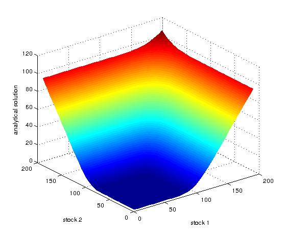
Figure 8: Analytical solution for option price at final time $T$. The computational domain of the problem is $\Omega=[0;300]\times[0;300]\times[0;T]$ with $T=1/12$, $K=100$, the volatilities $\sigma_{1}=\sigma_{2}=0.3$. The correlation coefficient is $\rho=0.5$, the risk free interest $r=0.03$ and $\Delta\tau=1/100$.

The graphs of option price with different methods are given in Figure 8,Figure 9 and Figure 10

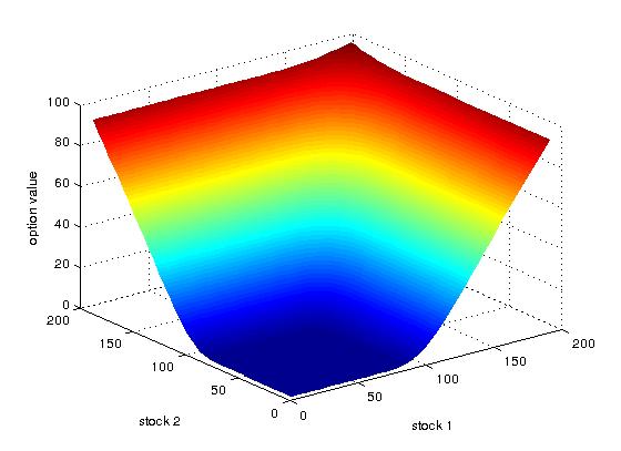
(a) MPFA-upwind 1st order

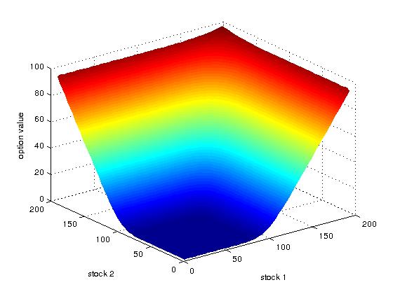
(b) MPFA-upwind 2nd order

Figure 9: Option price for MPFA-upwind methods at final time $T$. The computational domain of the problem is $\Omega=[0;300]\times[0;300]\times[0;T]$ with $T=1/12$, $K=100$, the volatilities $\sigma_{1}=\sigma_{2}=0.3$. The correlation coefficient is $\rho=0.5$, the risk free interest $r=0.03$ and $\Delta\tau=1/100$.

(a) fitted MPFA-upwind 1st order

(b) fitted MPFA-upwind 2nd order

Figure 10: Option price for fitted MPFA-upwind methods at final time $T$.The computational domain of the problem is $\Omega=[0;300]\times[0;300]\times[0;T]$ with $T=1/12$, $K=100$, the volatilities $\sigma_{1}=\sigma_{2}=0.3$. The correlation coefficient is $\rho=0.5$, the risk free interest $r=0.03$ and $\Delta\tau=1/100$.

In this paragraph, we consider the four numerical methods illustrated in the previous sections and the fitted finite volume method Huang et al. [2006]. We evaluate the error of these numerical method with respect to the analytical solution (5). The $L^{2}$-norm is used to compute the error as follows:

$$err=\frac{\sqrt{\sum_{i,j=1}^{N}meas(\mathcal{C}_{ij})\big{(}\mathcal{U}_{ij}-U_{ij}^{ana}\big{)}^{2}}}{\sqrt{\sum_{i,j=1}^{n}meas(\mathcal{C}_{ij})\big{(}U_{ij}^{ana}\big{)}^{2}}}$$ (101)

where $\mathcal{U}$ is the numerical solution, $U^{ana}$ the analytical solution and $meas(\mathcal{C}_{i,j})$ is the measure of the control volume $\mathcal{C}_{ij}$. This gives the following table:

	Fitted fin vol	MPFA-$1^{st}$ upw	MPFA-$2^{nd}$ upw	fitted MPFA-$1^{st}$ upw	fitted MPFA -$2^{nd}$ upw
$50\times 50$	0.0134	0.0060	0.0059	0.0060	0.0060
$70\times 70$	0.0133	0.0044	0.0044	0.0044	0.0044
$85\times 85$	0.0132	0.0037	0.0037	0.0037	0.0037
$100\times 100$	0.0132	0.0032	0.0032	0.0032	0.0032
$150\times 150$	0.0131	0.0024	0.0023	0.0023	0.0023

Table 1: Table of errors. The computational domain of the problem is $\Omega=[0;300]\times[0;300]\times[0;T]$ with $T=1/6$, $K=100$, the volatilities $\sigma_{1}=\sigma_{2}=0.3$. The correlation coefficient is $\rho=0.5$, the risk free interest $r=0.1$ and $\Delta\tau=1/100$.

	Fitted fin vol	MPFA-$1^{st}$ upw	MPFA-$2^{nd}$ upw	fitted MPFA-$1^{st}$ upw	fitted MPFA -$2^{nd}$ upw
$50\times 50$	0.0134	0.0060	0.0059	0.0060	0.0060
$100\times 100$	0.0104	0.0064	0.0063	0.0064	0.0063
$150\times 150$	0.0131	0.0056	0.0055	0.0056	0.0055

Table 2: Table of errors. The computational domain of the problem is $\Omega=[0;300]\times[0;300]\times[0;T]$ with $T=1/6$, $K=100$, the volatilities $\sigma_{1}=\sigma_{2}=0.3$. The correlation coefficient is $\rho=0.5$, the risk free interest $r=0.08$ and $\Delta\tau=1/100$.

	Fitted fin vol	MPFA-$1^{st}$ upw	MPFA-$2^{nd}$ upw	fitted MPFA-$1^{st}$ upw	fitted MPFA -$2^{nd}$ upw
$100\times 100$	0.0152	0.0239	0.0235	0.0240	0.0229
$150\times 150$	0.0151	0.0231	0.0228	0.0232	0.0229

Table 3: Table of errors. The computational domain of the problem is $\Omega=[0;300]\times[0;300]\times[0;T]$ with $T=1/6$, $K=100$, the volatilities $\sigma_{1}=\sigma_{2}=0.3$. The correlation coefficient is $\rho=0.5$ , the risk free interest $r=0$ and $\Delta\tau=1/100$.

	Fitted fin vol	MPFA-$1^{st}$ upw	MPFA-$2^{nd}$ upw	fitted MPFA-$1^{st}$ upw	fitted MPFA -$2^{nd}$ upw
$50\times 50$	0.1208	0.0631	0.0669	0.0623	0.0659
$100\times 100$	0.1203	0.0572	0.0648	0.0559	0.0629

Table 4: Table of errors. The computational domain of the problem is $\Omega=[0;4]\times[0;4]\times[0;T]$ with $T=2$, $K=1$, the volatilities $\sigma_{1}=\sigma_{2}=1$. The correlation coefficient is $\rho=0.3$, the risk free interest $r=0.5$ and $\Delta\tau=1/100$.

	Fitted fin vol	MPFA-$1^{st}$ upw	MPFA-$2^{nd}$ upw	fitted MPFA-$1^{st}$ upw	fitted MPFA -$2^{nd}$ upw
$50\times 50$	0.1196	0.0562	0.0643	0.0555	0.0624
$100\times 100$	0.1201	0.0626	0.0664	0.0618	0.0654

Table 5: Table of errors. The computational domain of the problem is $\Omega=[0;4]\times[0;4]\times[0;T]$ with $T=2$, $K=1$, the volatilities $\sigma_{1}=\sigma_{2}=1$. The correlation coefficient is $\rho=0.3$, the risk free interest $r=0.5$ and $\Delta\tau=1/10$.

As we can observe in Table 1-Table 5, the errors from our fitted MPFA and MPFA methods are smaller compared to those of fitted finite volume in Huang et al. [2006]. We can also note that when $r$ become smaller, the gaps between the errors of the fitted finite volume in Huang et al. [2006] and our fitted MPFA and MPFA methods reduce.

6 Conclusion

In this paper, we have presented the Multi-Point Flux Approximation (MPFA) to approximate the diffusion term of Black-Scholes Partial Differential Equation in its divergence form. The MPFA method coupled with the upwind methods (first and second order) have been used to solve numerically the Black-Scholes PDE. To handle the degeneracy of Black Scholes PDE, we have proposed a novel method based on a combination of the MPFA method and fitted finite volume by Huang et al. [2006]. We have performed some numerical simulations, which show that our fitted MPFA method coupled with first or second order upwinding methods are more accurate than the fitted finite volume method by Huang et al. [2006]. Rigorous convergence proof of the fitted MPFA will be our nearest future work.

References

- Aavatsmark [2002] Aavatsmark, I.(2002). An introduction to multipoint flux approximations for quadrilateral grids. Computational Geosciences, 6(3-4):405–432.
- Aavatsmark [2007] Aavatsmark, I. (2007) Multipoint flux approximation methods for quadrilateral grids. In 9th International forum on reservoir simulation, Abu Dhabi, pages 9–13.
- Angermann and Wang [2007] Angermann, L. & Wang, S.(2007). Convergence of a fitted finite volume method for the penalized black–scholes equation governing european and american option pricing. Numerische Mathematik, 106(1):1–40.
- Bates [1996] Bates, D. S.(1996). Jumps and stochastic volatility: Exchange rate processes implicit in deutsche mark options. The Review of Financial Studies, 9(1):69–107.
- Duffy [2013] Duffy, D. J. (2013) Finite Difference methods in financial engineering: A Partial Differential Equation approach. John Wiley & Sons.
- Haug [2007] Haug., E. G. (2007). The complete guide to option pricing formulas, volume 2. McGraw-Hill New York.
- Heston [1993] Heston, S. L. (1993). A closed-form solution for options with stochastic volatility with applications to bond and currency options. The review of financial studies, 6(2):327–343.
- Huang et al. [2006] Huang, C-S., Hung,C-H., & Wang, S.(2006). A fitted finite volume method for the valuation of options on assets with stochastic volatilities. Computing, 77(3):297–320.
- Huang et al. [2009] Huang, C-S., Hung,C-H., & Wang, S.(2009). On convergence of a fitted finite-volume method for the valuation of options on assets with stochastic volatilities. IMA journal of numerical analysis, 30(4):1101–1120.
- Hull [2003] Hull, J. C. (2003) Options, futures and others. Derivative (Fifth Edition), Prentice Hall.
- Kwok [2008] Kwok, Y.-K.(2008). Mathematical models of financial derivatives. Springer.
- LeVeque [2004] LeVeque, R. J. (2004). Finite volume methods for hyperbolic problems. Cambridge Texts in Applied Mathematics, 39(1):88–89.
- Lie et al. [2012] Lie K.-A., Krogstad, S., Ligaarden I., S. , Natvig ,J. R., Nilsen, H. M., & Bård Skaflestad, B.(2012). Open-source matlab implementation of consistent discretisations on complex grids. Computational Geosciences, 16(2):297–322.
- Persson and Sydow [2007] Persson, J., & Sydow, L. V. (2007). Pricing European multi-asset options using a space-time adaptive FD-method. Computing and Visualization in Science, 10(4):173–183.
- Sandve et al. [2012] Sandve, T. H., Berre, I., & Nordbotten, J. M.(2012) An efficient multi-point flux approximation method for discrete fracture–matrix simulations. Journal of Computational Physics, 231(9):3784–3800.
- Stephansen [2012] Stephansen, A. F.(2012). Convergence of the multipoint flux approximation l-method on general grids. SIAM Journal on Numerical Analysis, 50(6):3163–3187.
- Tambue [2016] Tambue, A. (2016). An exponential integrator for finite volume discretization of a reaction–advection–diffusion equation. Computers & Mathematics with Applications, 71(9):1875–1897.
- Wang [2004] Wang, S.(2004). A novel fitted finite volume method for the black–scholes equation governing option pricing. IMA Journal of Numerical Analysis, 24(4):699–720.
- Wilmott [2005] Wilmott, P. (2005) The Best of Wilmott 1: Incorporating the Quantitative Finance Review. John Wiley & Sons.
- Wilmott et al. [1993] Wilmott, P., Dewynne, J., & Howison , S. (1993). Option pricing: mathematical models and computation. Oxford financial press.