Scalable and Efficient Comparison-based Search without Features

Abstract

We consider the problem of finding a target object $t$ using pairwise comparisons, by asking an oracle questions of the form “Which object from the pair $(i,j)$ is more similar to $t$?”. Objects live in a space of latent features, from which the oracle generates noisy answers. First, we consider the non-blind setting where these features are accessible. We propose a new Bayesian comparison-based search algorithm with noisy answers; it has low computational complexity yet is efficient in the number of queries. We provide theoretical guarantees, deriving the form of the optimal query and proving almost sure convergence to the target $t$. Second, we consider the blind setting, where the object features are hidden from the search algorithm. In this setting, we combine our search method and a new distributional triplet embedding algorithm into one scalable learning framework called Learn2Search. We show that the query complexity of our approach on two real-world datasets is on par with the non-blind setting, which is not achievable using any of the current state-of-the-art embedding methods. Finally, we demonstrate the efficacy of our framework by conducting an experiment with users searching for movie actors.

1 Introduction

Finding a target object among a large collection of $n$ objects is the central problem addressed in information retrieval (IR). For example, in web search, one finds relevant web pages through a query expressed as one or several keywords. Of course, the form of the query depends on the object type; other forms of search queries in the literature include finding images similar to a query image (Datta et al., 2008), and finding subgraphs of a large network isomorphic to a query graph (Sun et al., 2012). A common feature of this classic formulation of the search problem is the need to express a meaningful query. However, this is often a non-trivial task for a human user. For example, most people would struggle to draw the face of a friend accurately enough that it could be used as a query image. But they would be able to confirm with near-total certainty whether a photograph is of their friend—we have no real doppelgängers in the world. In other words, comparing is cognitively much easier than formulating a query. This is true for many complex or unstructured types of data, such as music, abstract concepts, images, videos, flavors, etc.

In this work, we develop models and algorithms for searching a large database by comparing a sequence of sample objects relative to the target, thereby obviating the need for any explicit query. The central problem concerns the choice of the sequence of samples (e.g., pairs of faces that the user compares with a target face she remembers). These query objects have to be chosen in such a way that we learn as much as possible about the target, i.e., shrink the set of potential targets as quickly as possible. This is closely related to a classic problem in active learning (Settles, 2012; MacKay, 1992), assuming we have a meaningful set of features available for each object in the database.

It is natural to assume that the universe of objects lives in some low-dimensional latent feature space, even though the raw objects might be high-dimensional (images, videos, sequences of musical notes, etc.). For example, a human face, for the purposes of a similarity comparison, could be quite accurately described by a few tens of features, capturing head shape, eye color, fullness of lips, gender, age, and the like (Chang & Tsao, 2017).

The key component of our framework is a noisy oracle model that describes how a user responds to comparison queries relative to a target, based on the objects’ embedding in the latent feature space. The noise model implicitly determines which queries are likely to extract useful information from the user; it is similar to pairwise comparison models such as those of Thurstone (1927) or Bradley & Terry (1952), but here the comparison is always relative to a target. The compared samples and the target are all represented as points in the feature space. Our contributions in this context are threefold. First, we develop an efficient search algorithm, which (a) generates query pairs and (b) navigates towards the target. This algorithm is provably guaranteed to converge to the target, due to the specific form of our comparison model and key properties of the search algorithm. In contrast with prior adaptive search methods, where generating a query pair is typically expensive, our algorithm is also computationally efficient.

We also consider the more difficult, but realistic, scenario where the objects still live in a low-dimensional feature space, but the search algorithm does not have access to their embedding. In this blind setting, the latent features of an object manifest themselves only through the comparison queries. Although this assumption clearly makes the problem challenging, it also has the advantage of yielding a completely generic approach. We develop a method to generate a latent embedding of the objects from past searches, in order to make future searches more efficient. The goal of the method is to minimize the number of queries to locate a target; this is achieved by gradually improving the latent embedding of all the objects based on past searches. Unlike with previous triplet embedding approaches that use low-dimensional point estimates to represent objects, we embed each object as a Gaussian distribution, which captures the uncertainty in the exact position of the object given the data. We show that our approach leads to significant gains in a real-world application, where users search for movie actors by comparing faces: Our framework learns useful low-dimensional representations based on comparison outcomes that lead to decreasing search cost as more data is collected.

The rest of the paper is structured as follows. In Section 2, we give an overview of related work. In Section 3, we define the problem of comparison-based search and define our user (oracle) model. In Section 4, we describe our interactive search method in the non-blind setting, establish its favorable scalability, and prove its convergence properties. In Section 5, we focus on the blind setting, and introduce our distributional embedding method GaussEmbed and its integration into the combined Learn2Search framework. We demonstrate the performance of our algorithms on synthetic and real world datasets in Section 6 in both non-blind and blind settings, and also present the results of an experiment invloving human oracles searching for movie. Finally, we give our concluding remarks in Section 7. For conciseness, we defer the full proofs of our theorems to the supplementary material.

2 Related Work

Comparison-Based Search.

For the general active learning problem, where the goal is to identify a target hypothesis by making queries, the Generalized Binary Search method (Dasgupta, 2005; Nowak, 2008) is known to be near-optimal in the number of queries if the observed outcomes are noiseless. In the noisy case, Nowak (2009) and Golovin et al. (2010) propose objectives that are greedily minimized over all possible queries and outcomes in a Bayesian framework with a full posterior distribution over the hypothesis. We adapt the method suggested by Golovin et al. (2010) to our setting and investigate its performance in comparison to the one proposed in this paper later in Section 6.

Adaptive search through relevance feedback by using preprocessed features was studied in the context of image retrieval systems by Cox et al. (2000); Fang & Geman (2005); Ferecatu & Geman (2009); Suditu & Fleuret (2012) in a Bayesian framework and by using different user answer models.

When the features are hidden, finding a target in a set of objects by making similarity queries is explored by Tschopp et al. (2011) and Karbasi et al. (2012) in the noiseless case. To deal with erroneous answers, Kazemi et al. (2018) consider an augmented user model that allows a third outcome to the query, “?”; it can be used by a user to indicate that they do not know the answer confidently. With this model, they propose several new search techniques under different assumptions on the knowledge of relative object distances. Karbasi et al. (2012) also briefly discussed the case of a noisy oracle with a constant mistake probability and proposed to treat it with repeated queries. Haghiri et al. (2017) consider the problem of nearest-neighbor search using comparisons in the noiseless setting.

Brochu et al. (2008) study the comparison-based search problem in continuous space. Their approach relies on maximizing a surrogate GP model of the valuation function. In contrast to their work, our approach is restricted to a specific valuation function (based on the distance to the target), but our search algorithm is backed by theoretical guarantees, its running time is independent of the number of queries and scales better with the number of objects. Chu & Ghahramani (2005) and Houlsby et al. (2011) study a similar problem where the entire valuation function needs to be estimated. Our approach is inspired from this line of work and also uses the expected information gain to drive the search algorithm. However, our exact setup enables finding a near-optimal query pair simply by evaluating a closed-form expression, as opposed to searching exhaustively over all pairs of objects. Comparison-based search under noise is also explored in Canal et al. (2019); the authors independently propose an oracle model similar to ours.

Triplet Embedding.

The problem of learning objects embedding based on triplet comparisons has been studied extensively in recent years. Jamieson & Nowak (2011) provides a lower bound on the number of triplets needed to uniquely determine an embedding that satisfies all $O(n^{3})$ relational constraints and describe an adaptive scheme that builds an embedding by sequentially selecting triplets of objects to compare.

More general algorithms for constructing ordinal embeddings from a given set of similarity triplets, under different triplet probability models, are proposed by Agarwal et al. (2007), Tamuz et al. (2011) and Van Der Maaten & Weinberger (2012). Amid & Ukkonen (2015) modify the optimization problem of Van Der Maaten & Weinberger (2012) to learn at once multiple low-dimensional embeddings, each corresponding to a single latent feature of an object. Theoretical properties for a general maximum likelihood estimator with an assumed probabilistic generative data model are studied by Jain et al. (2016).

An alternative approach to learning ordinal data embedding is suggested in Kleindessner & von Luxburg (2017), where the authors explicitly construct kernel functions to measure similarities between pairs of objects based on the set of triplet comparisons. Finally, Heim et al. (2015) adapt the kernel version of Van Der Maaten & Weinberger (2012) for an online setting, when the set of observable triplets is expanding over time. The authors use stochastic gradient descent to learn the kernel matrix and to exploit sparsity properties of the gradient. Although this work is closely related to our scenario, the kernel decomposition, which is $O(n^{3})$ in time, would be too computationally expensive to perform in the regimes of interest to us.

Finally, Ghosh et al. (2019) and Anderton & Aslam (2019) both propose landmark-based triplet embedding methods that scale well for large values of $n$ but assume direct access to the oracle in order to ask to compare adaptively selected triplets.

3 Preliminaries

Let us consider $n$ objects denoted by integers $[n]=\{1,2,\dots,n\}$. Our goal is to build an interactive comparison-based search engine that would assist users in finding their desired target object $t\in[n]$ by sequentially asking questions of the form “among the given pair of objects $(i,j)$, which is closer to your target?” and observing their answers $y\in\{i,j\}$. Formally, at each step of this search, we collect an answer $y$ to the query $(i,j)$. We then use this information to decide on the next pair of objects $(i^{\prime},j^{\prime})$ to show to the user, until one of the elements in the query is recognized as the desired target.

We assume that the objects have associated latent feature vectors $\mathcal{X}=\{{\bm{x}}_{1},{\bm{x}}_{2},\dots,{\bm{x}}_{n}\},{\bm{x}}_{i}\in\mathbb{R}^{d}$, that reflect their individual properties and that are intuitively used by users when answering the queries. In fact, each user response $y$ can be viewed as an outcome of a perceptual judgement on the similarity between objects that is based on these representations. A natural choice of quantifying similarities between objects is the Euclidean distance between hidden vectors in $\mathbb{R}^{d}$:

$$y(i,j\leavevmode\nobreak\ |\leavevmode\nobreak\ t)=i\leavevmode\nobreak\ \leavevmode\nobreak\ \iff\leavevmode\nobreak\ \leavevmode\nobreak\ ||{\bm{x}}_{i}-{\bm{x}}_{t}||<||{\bm{x}}_{j}-{\bm{x}}_{t}||.$$

Different users might have slightly different perceptions of similarity. Even for a single user, it might be difficult to answer every comparison confidently, and as such we might observe inconsistencies across their replies. We postulate that this happens when two objects ${\bm{x}}_{i}$ and ${\bm{x}}_{j}$ are roughly equidistant from the target ${\bm{x}}_{t}$, and less likely when the distances are quite different. In other words, answers are most noisy when the target is close to the decision boundary, i.e., the bisecting normal hyperplane to the segment between ${\bm{x}}_{i}$ and ${\bm{x}}_{j}$, and less noisy when it is far away from it.

We consider the following probabilistic model that captures the possible uncertainty in users’ answers (probit model):

$$p(y(i,j\leavevmode\nobreak\ |\leavevmode\nobreak\ t)=i) =p({\bm{x}}_{t}^{T}{\bm{w}}_{ij}+b_{ij}+\varepsilon>0)$$

$$=\Phi\left(\frac{{\bm{x}}_{t}^{T}{\bm{w}}_{ij}+b_{ij}}{\sigma_{\varepsilon}}\right),$$ (1)

where ${\bm{x}}_{i},{\bm{x}}_{j},{\bm{x}}_{t}\in\mathbb{R}^{d}$ are the coordinates of the query points and the target, respectively,

$$h_{ij}=({\bm{w}}_{ij},b_{ij})=\left(\frac{{\bm{x}}_{i}-{\bm{x}}_{j}}{\lVert{\bm{x}}_{i}-{\bm{x}}_{j}\rVert},\frac{\|{\bm{x}}_{j}\rVert^{2}-\lVert{\bm{x}}_{i}\rVert^{2}}{2\lVert{\bm{x}}_{i}-{\bm{x}}_{j}\rVert}\right)$$

is the bisecting normal hyperplane to the segment between ${\bm{x}}_{i}$ and ${\bm{x}}_{j}$, $\varepsilon\sim\mathcal{N}(0,\sigma_{\varepsilon}^{2})$ is additive Gaussian noise, and $\Phi$ is the Standard Normal CDF. Indeed, if ${\bm{x}}_{t}$ is on the hyperplane $h_{ij}$, the answers to queries are pure coin flips, as the target point is equally far from both query points. Everywhere else answers are biased toward the correct answer, and the probability of the correct answer depends only on the distance of ${\bm{x}}_{t}$ to the hyperplane $h_{ij}$.

This model is reminiscent of pairwise comparison models such as those of Thurstone (1927) or Bradley & Terry (1952), e.g., where $p(y(i,j\leavevmode\nobreak\ |\leavevmode\nobreak\ t)=i)=\Phi[s({\bm{x}}_{i})-s({\bm{x}}_{j})]$ and $s({\bm{x}})=-\lVert{\bm{x}}-{\bm{x}}_{t}\rVert_{2}^{2}$ (Agarwal et al., 2007; Jain et al., 2016). These models have the undesirable property of favoring distant query points: given any ${\bm{x}}_{i},{\bm{x}}_{j}\neq\bm{0}$, it is easy to verify that the pair $(2{\bm{x}}_{i},2{\bm{x}}_{j})$ is strictly more discriminative for any target that does not lie on the bisecting hyperplane. Our comparison model is different: in (1), the outcome probability depends on ${\bm{x}}_{i}$ and ${\bm{x}}_{j}$ only through their bisecting hyperplane.

4 Search with Known Features

In this section, we describe our algorithm for interactive search in a set of objects $[n]$ when we have access to the features $\mathcal{X}$. We are interested in methods that are (a) efficientin the average number of queries per search, and (b) scalablein the number of objects. Scalability requires low computational complexity of the procedure for choosing the next query. As we expect users to make mistakes in their answers, we also require our algorithms to be robust to noise in the human feedback.

Gaussian Model.

Due to the sequential and probabilistic nature of the problem, we take a Bayesian approach in order to model the uncertainty about the location of the target. In particular, we maintain a $d$-dimensional Gaussian distribution $\mathcal{N}(\hat{{\bm{x}}};{\bm{\mu}},{\bm{\Sigma}})$ that reflects our current belief about the position of the target point ${\bm{x}}_{t}$ in $\mathbb{R}^{d}$. We model user answers with the probit likelihood (1), and we apply approximate inference techniques for updating ${\bm{\mu}}$ and ${\bm{\Sigma}}$ every time we observe a query outcome. The space requirement of the model is $O(d^{2})$.

The motivation behind such a choice of parametrization is that (a) the size of the model does not depend on $n$, guaranteeing scalability, (b) one can characterize a general pair of points in $\mathbb{R}^{d}$ that maximizes the expected information gain, and (c) the sampling scheme that chooses the next pair of query points informed by (b) is simple and works extremely well in practice.

4.1 Choosing the Next Query

To generate the next query, we follow a classical approach from information-theoretic active learning (MacKay, 1992): find the query that minimizes the expected posterior uncertainty of our estimate $\hat{{\bm{x}}}$, as given by its entropy. More specifically, we find a pair of points $({\bm{x}}_{i},{\bm{x}}_{j})$ that maximizes the expected information gain for our current estimation of ${\bm{x}}_{t}$ at step $m$:

$$I[\hat{{\bm{x}}};y\mid({\bm{x}}_{i},{\bm{x}}_{j})]=H(\hat{{\bm{x}}})-\mathbb{E}_{y\mid\hat{{\bm{x}}},{\bm{x}}_{i},{\bm{x}}_{j}}[H(\hat{{\bm{x}}}\mid y)],$$

where $\hat{{\bm{x}}}\sim\mathcal{N}({\bm{\mu}},{\bm{\Sigma}})$ is the current belief about the target position and $y\sim p(y\mid\hat{{\bm{x}}},{\bm{x}}_{i},{\bm{x}}_{j})$ is the current belief over the answer to the comparison between ${\bm{x}}_{i}$ and ${\bm{x}}_{j}$.

Exhaustively evaluating the expected information gain over all $O(n^{2})$ pairs for each query (e.g., as done in Chu & Ghahramani, 2005) is prohibitively expensive. Instead, we propose a more efficient approach. Recall from equation (1) that the comparison outcome probability $p(y\mid\hat{{\bm{x}}},{\bm{x}}_{i},{\bm{x}}_{j})$ depends on $({\bm{x}}_{i},{\bm{x}}_{j})$ only through the corresponding bisecting normal hyperplane $h_{ij}$. Therefore, instead of looking for the optimal pair of points from $\mathcal{X}$, we first find the hyperplane $h$ that maximizes the expected information gain. Following Houlsby et al. (2011), it can be rewritten as:

$$I[\hat{{\bm{x}}};y\mid h] =H(\hat{{\bm{x}}})-\mathbb{E}_{y\mid\hat{{\bm{x}}},h}[H(\hat{{\bm{x}}}\mid y)]$$

$$=H(y\mid\hat{{\bm{x}}},h)-\mathbb{E}_{\hat{{\bm{x}}}}[H(y\mid\hat{{\bm{x}}},h)].$$ (2)

The following theorem gives us the key insight about the general form of a hyperplane $h=({\bm{w}},b)$ that optimizes this utility function by splitting the Gaussian distribution into two equal “halves”:

Theorem 1.

Let $\hat{{\bm{x}}}\sim\mathcal{N}({\bm{\mu}},{\bm{\Sigma}})$, and let $\mathcal{H}=\{({\bm{w}},b)\mid\lVert{\bm{w}}\rVert=1,{\bm{w}}^{T}{\bm{\mu}}+b=0\}$ be the set of all hyperplanes passing through ${\bm{\mu}}$. Then,

$$\operatorname*{arg\,max}_{h\in\mathcal{H}}I[\hat{{\bm{x}}};y\mid h]=\operatorname*{arg\,max}_{({\bm{w}},b)\in\mathcal{H}}{\bm{w}}^{T}{\bm{\Sigma}}{\bm{w}}.$$

Proof sketch.

Let $h^{\star}=({\bm{w}}^{\star},b^{\star})$ be an optimal hyperplane. Since ${\bm{w}}^{T}{\bm{\mu}}+b=0$, we have $p(y\mid\hat{{\bm{x}}},h)\equiv 1/2$ and $H(y\mid\hat{{\bm{x}}},h)\equiv 1$. Thus, $h^{\star}$ is such that $\mathbb{E}_{\hat{{\bm{x}}}}[H(y\mid\hat{{\bm{x}}},h)]$ is minimal. We show that

$$\mathbb{E}_{\hat{{\bm{x}}}}[H(y\mid\hat{{\bm{x}}},h)]=\mathbb{E}_{z}[H(\Phi(z))],$$

where $z\sim\mathcal{N}(0,{\bm{w}}^{T}{\bm{\Sigma}}{\bm{w}})$. As the binary entropy function has a single maximum in $1/2$, the expectation on the r.h.s. is minimized when the variance of $z$ is maximized. ∎

In other words, Theorem 1 states that any optimal hyperplane is orthogonal to a direction that maximizes the variance of $\hat{{\bm{x}}}$.

Consequently, we find a hyperplane $h$ that maximizes the expected information gain via an eigenvalue decomposition of ${\bm{\Sigma}}$. However, we still need to find a pair of objects $(i,j)$ to form the next query. We propose a sampling strategy based on Theorem 1, which we describe in Algorithm 1. After computing the optimal hyperplane $h^{\star}$, we sample a point ${\bm{z}}_{1}$ from the current Gaussian belief over the location of the target, and reflect it across $h^{\star}$ to give the second point ${\bm{z}}_{2}$. Then our query is the closest pair of (distinct) unused points $({\bm{x}}_{i},{\bm{x}}_{j})$ from the dataset to $({\bm{z}}_{1},{\bm{z}}_{2})$.

Assuming that the feature vectors $\mathcal{X}$ are organized into a $k$-d tree (Bentley, 1975) at a one-time computational cost of $O(n\log{n})$ for a given $\mathcal{X}$, Algorithm 1 runs in time $O(\log{n}+d^{3})$. This includes $O(d^{3})$ for the eigenvalue decomposition, $O(d^{2})$ for sampling from a $d$-dimensional Gaussian distribution, $O(d)$ for mirroring the sample, and $O(\log{n})$ on average for finding the closest pair of points from the dataset using the $k$-d tree.

If needed, computing the eigenvector that corresponds to the largest eigenvalue can be well approximated via the power method with $O(d^{2})$ complexity (assuming a constant number of iterations). This will bring down the total complexity of Algorithm 1 to $O(\log{n}+d^{2})$.

Algorithm 1 SampleMirror

0:  current belief $\mathcal{N}({\bm{\mu}},{\bm{\Sigma}})$, $\mathcal{X}$, $\mathcal{U}$

0:  query pair $({\bm{x}}_{i},{\bm{x}}_{j})$

1:  Compute optimal hyperplane $h^{\star}$ for $({\bm{\mu}},{\bm{\Sigma}})$.

2:  Sample a point ${\bm{z}}_{1}$ from $\mathcal{N}({\bm{\mu}},{\bm{\Sigma}})$.

3:  Obtain ${\bm{z}}_{2}$, as the reflection of ${\bm{z}}_{1}$ across $h^{\star}$.

4:  Find objects $i$ and $j$, s.t. $i\neq j$ and $i,j\not\in\mathcal{U}$, with the closest representations ${\bm{x}}_{i}$ and ${\bm{x}}_{j}$ to ${\bm{z}}_{1}$ and ${\bm{z}}_{2}$, respectively.

Note that the actual hyperplane defined by the obtained pair $({\bm{x}}_{i},{\bm{x}}_{j})$ in Algorithm 1 does not, in general, coincide with the optimal one. Nevertheless, the hyperplane $h_{ij}$ approximates $h^{\star}$ increasingly better as $n$ grows.

4.2 Updating the Model

Finally, after querying the pair $(i,j)$ and observing outcome $\bar{y}$, we update our belief on the location of target $\hat{{\bm{x}}}$. Suppose that we are at the $m$-th step of the search, and denote the belief before observing $\bar{y}$ by $p_{m-1}(\hat{{\bm{x}}})=\mathcal{N}(\hat{{\bm{x}}};{\bm{\mu}}_{m-1},{\bm{\Sigma}}_{m-1})$. Ideally, we would like to update it using

$$p^{\star}_{m}(\hat{{\bm{x}}})\propto p(y=\bar{y}\mid{\bm{x}}_{i},{\bm{x}}_{j},\hat{{\bm{x}}})\cdot p_{m-1}(\hat{{\bm{x}}}).$$

However, this distribution is no longer Gaussian. Therefore, we approximate it by the “closest” Gaussian distribution $p_{m}(\hat{{\bm{x}}})\doteq\mathcal{N}(\hat{{\bm{x}}};{\bm{\mu}}_{m},{\bm{\Sigma}}_{m})$. We use a method known as assumed density filtering (Minka, 2001), which solves the following program:

$$\min_{{\bm{\mu}}_{m},{\bm{\Sigma}}_{m}}D_{\mathrm{KL}}\left[p^{\star}_{m}(\hat{{\bm{x}}})\ \|\ p_{m}(\hat{{\bm{x}}})\right],$$

where $D_{\mathrm{KL}}[p\|q]$ is the Kullback-Leibler divergence from $p$ to $q$. This can be done in closed form by computing the first two moments of the distribution $p^{\star}_{m}$, with running time $O(d^{2})$. Formally, at each step of the search, we perform the following computations (referred to further as the Update routine):

$$\begin{aligned} {\bm{\Sigma}}_{m}&=\left({\bm{\Sigma}}_{m-1}^{-1}+\tau{\bm{w}}{\bm{w}}^{T}\right)^{-1},\\ {\bm{\mu}}_{m}&={\bm{\Sigma}}_{m}[{\bm{\Sigma}}_{m-1}^{-1}{\bm{\mu}}_{m-1}+(\nu-b\tau){\bm{w}}],\end{aligned}$$

$$\tau=\frac{-\beta}{1+\beta{\bm{w}}^{T}{\bm{\Sigma}}_{m-1}{\bm{w}}},\quad\nu=\frac{\alpha-\beta({\bm{\mu}}_{m-1}^{T}{\bm{w}}+b)}{1+\beta{\bm{w}}^{T}{\bm{\Sigma}}_{m-1}{\bm{w}}},$$

where $\alpha$ and $\beta$ are the first and second derivatives with respect to $\mu={\bm{\mu}}_{m-1}^{T}{\bm{w}}_{ij}$ of the log-marginal likelihood

$$\log\int_{\mathbb{R}^{d}}p(\bar{y})p(\hat{{\bm{x}}})d\hat{{\bm{x}}}=\log\Phi\left(\frac{{\bm{\mu}}_{m-1}^{T}{\bm{w}}+b}{\sqrt{{\bm{w}}^{T}{\bm{\Sigma}}_{m-1}{\bm{w}}+\sigma_{\varepsilon}^{2}}}\right).$$

We summarize the full active search procedure in Algorithm 2.

Algorithm 2 GaussSearch

0:  Objects $[n]$, feature vectors $\mathcal{X}$.

0:  target object $t$

1:  Initialize ${\bm{\mu}}_{0}$ and ${\bm{\Sigma}}_{1}$

2:  $\mathcal{U}\leftarrow\emptyset$

3:  $m\leftarrow 1$

4:  repeat

5:     ${\bm{x}}_{i},{\bm{x}}_{j}\leftarrow\textsc{SampleMirror}({\bm{\mu}}_{m-1},{\bm{\Sigma}}_{m-1},\mathcal{X},\mathcal{U})$

6:     $\mathcal{U}\leftarrow\mathcal{U}\cup\{i,j\}$

7:     $\bar{y}\leftarrow$ noisy comparison outcome as per (1)

8:     ${\bm{\mu}}_{m},{\bm{\Sigma}}_{m}\leftarrow\textsc{Update}({\bm{x}}_{i},{\bm{x}}_{j},\bar{y},{\bm{\mu}}_{m-1},{\bm{\Sigma}}_{m-1}$)

9:     $m\leftarrow m+1$

10:  until $t\in\{i,j\}$

4.3 Convergence of GaussSearch

For finite $n$, GaussSearch is guaranteed to terminate because samples are used without repetition. However, in a scenario where $n$ is effectively infinite because the feature space is dense, i.e., $\mathcal{X}=\mathbb{R}^{d}$, we are able to show a much stronger result. The following theorem asserts that, for any initial Gaussian prior distribution over the target with full-rank covariance matrix, the GaussSearch posterior asymptotically concentrates at the target.

Theorem 2.

If the answers follow (1), then for any initial $\bm{\mu}_{0}$ and $\bm{\Sigma}_{0}\succ 0$, as $m\to\infty$ we have

1. $\operatorname{Tr}({\bm{\Sigma}}_{m})\to 0$,

2. ${\bm{\mu}}_{m}\to{\bm{x}}_{t}$

almost surely.

Proof sketch.

We obtain crucial insights on the asymptotic behavior by studying the case $d=1$, when ${\bm{x}}_{t}$, ${\bm{\mu}}_{m}$ and ${\bm{\Sigma}}_{m}$ become scalars $x_{t}$, $\mu_{m}$ and $\sigma^{2}_{m}$, respectively. We first show that $\sigma^{2}_{m}=\Theta(1/m)$. Next, we are able to recast $\{\mu_{m}\}_{m=0}^{\infty}$ as a random walk biased towards $x_{t}$, with step size $\sigma^{2}_{m}$. By drawing on results from stochastic approximation theory (Robbins & Monro, 1951; Blum et al., 1954), we can show that $\mu_{m}\to x_{t}$ almost surely. The extension to $d>1$ follows by noticing that, in the dense case $\mathcal{X}=\mathbb{R}^{d}$, we can assume (without loss of generality) that the search sequentially iterates over each dimension in a round-robin fashion. ∎

This result is not a priori obvious, especially in light of the model for the oracle: answers become coin flips as the sample points ${\bm{x}}_{i}$ and ${\bm{x}}_{j}$ get closer. Nevertheless, Theorem 2 guarantees that the algorithm continues making progress towards the target.

5 Search with Latent Features

In this section, we relax the assumption that the feature vectors $\mathcal{X}$ are available; instead, we consider the blind scenario, where $\mathcal{X}$ is only used implicitly by the oracle to generate answers to queries. As a consequence, we need to generate an estimated feature embedding $\hat{\mathcal{X}}=\{\hat{{\bm{x}}}_{1},\ldots,\hat{{\bm{x}}}_{n}\}$ from comparison data collected from past searches. As we collect more data, the embedding $\hat{\mathcal{X}}$ should gradually approximate the true embedding $\mathcal{X}$ (up to rotation and reflection), improving the performance of future searches.

In a given dataset of triplet comparison outcomes, one item might be included in few triplets while another might be included in many (e.g., due to the latter being a popular search target), thus we could have more information about one item and less information about another. This suggests that when approximating $\mathcal{X}$, an uncertainty about the item’s position should be taken into account. The latest should also affect the operation of the search algorithm: After observing the outcome of oracle’s comparison between two objects $i$ and $j$, whose positions $\hat{{\bm{x}}}_{i}$ and $\hat{{\bm{x}}}_{j}$ in our estimated embedding space are noisy, the target posterior distribution should have higher entropy than if $\hat{{\bm{x}}}_{i}$ and $\hat{{\bm{x}}}_{j}$ were exact (as we had assumed so far).

We incorporate this dependence by generating a distributional embedding, where each estimate $\hat{{\bm{x}}}_{i}$ is endowed with a distribution, thus capturing the uncertainty about its true position ${\bm{x}}_{i}$. We also slightly modify the posterior update step (line 8 in Algorithm 2) in the search algorithm, in order to reflect the embedding uncertainty in the belief about the target. We refer to this combined learning framework as Learn2Search. It combines GaussSearch, our search method from the previous section, with a new triplet embedding technique called GaussEmbed. We now describe our distributional embedding method, then give a brief description of the combined framework.

5.1 Distributional Embedding

As before, suppose we are given a set of objects $[n]=\{1,2,\dots,n\}$, known to have representations $\mathcal{X}\subset\mathbb{R}^{d}$ in a hidden feature space. Although we do not have access to $\mathcal{X}$, we observe a set of noisy triplet-based relative similarities of these objects: $\mathcal{T}=\{(i,j;k)\mid\text{object $i$ is closer to $k$ than $j$ is}\},$ obtained w.r.t. probabilistic model (1). The goal is to learn a $d$-dimensional Gaussian distribution embedding

$$q(\hat{{\bm{x}}}_{1},\hat{{\bm{x}}}_{2},\dots,\hat{{\bm{x}}}_{n})\doteq\prod_{i}\mathcal{N}(\hat{{\bm{x}}}_{i};{\bm{\nu}}_{i},{\bm{\Psi}}_{i})$$

where ${\bm{\nu}}_{i}\in\mathbb{R}^{d}$, ${\bm{\Psi}}_{i}\in\mathbb{R}^{d\times d}$ and diagonal, such that objects that are similar w.r.t. their “true” representations $\{{\bm{x}}_{i}\}_{i=1}^{n}$ (reflected by $\mathcal{T}$) are also similar in the learned embedding. Here for each object, ${\bm{\nu}}_{i}$ represents the mean guess on the location of object $i$ in $\mathbb{R}^{d}$, and ${\bm{\Psi}}_{i}$ represents the uncertainty about its position.

We learn this Gaussian embedding via maximizing the Evidence Lower Bound (ELBO),

$$\mathcal{L}=\mathbb{E}_{q}\left[\log{p(\mathcal{T},\hat{{\bm{x}}}_{1},\ldots,\hat{{\bm{x}}}_{n})}-\log{q(\hat{{\bm{x}}}_{1},\ldots,\hat{{\bm{x}}}_{n})}\right],$$ (3)

where the joint distribution $p(\mathcal{T},\hat{{\bm{x}}}_{1},\ldots,\hat{{\bm{x}}}_{n})$ is the product of the prior $p(\hat{{\bm{x}}}_{1},\ldots,\hat{{\bm{x}}}_{n})=\prod_{i}\mathcal{N}(\hat{{\bm{x}}}_{i};\bm{0},{\bm{I}})$ and the likelihood $p(\mathcal{T}\mid\hat{{\bm{x}}}_{1},\ldots,\hat{{\bm{x}}}_{n})$ given w.r.t. the probabilistic model (1) with $\sigma_{\varepsilon}=1$. We optimize the ELBO by using stochastic backpropagation with the reparametrization trick (Kingma & Welling, 2014; Rezende et al., 2014). The total complexity of executing one epoch is $O(|\mathcal{T}|d)$.

5.2 Learning to Search

We now describe our joint embedding and search framework, Learn2Search. We begin by initializing $\hat{\mathcal{X}}$ to its prior distribution, $\prod_{i}\mathcal{N}(\hat{{\bm{x}}}_{i};\bm{0},{\bm{I}})$. Then we alternate between searching and updating the embedding, based on all the comparison triplets collected in previous searches, by (a) running GaussSearch on the estimated embedding $\hat{\mathcal{X}}$, and (b) running GaussEmbed to refine $\hat{\mathcal{X}}$ based on all triplets observed so far. The distributional embedding requires the following modifications in GaussSearch.

1. in SampleMirror, we use the Mahalanobis distance $({\bm{\nu}}-{\bm{z}})^{T}{\bm{\Psi}}^{-1}({\bm{\nu}}-{\bm{z}})$ when finding the closest objects $i,j$ to the sampled points ${\bm{z}}_{1},{\bm{z}}_{2}$.

2. in the Update step, we combine the variance of the noisy outcome $\sigma^{2}_{\varepsilon}$ with the uncertainty over the location of $\hat{{\bm{x}}}_{i}$ and $\hat{{\bm{x}}}_{j}$ along the direction perpendicular to the hyperplane, resulting in an effective noise variance $\sigma_{\text{eff}}^{2}=\sigma_{\varepsilon}^{2}+{\bm{w}}^{T}{\bm{\Psi}}_{i}{\bm{w}}+{\bm{w}}^{T}{\bm{\Psi}}_{j}{\bm{w}}$.

Both modifications results in a natural tradeoff between exploration and exploitation: At first, we tend to sample uncertain points more frequently, and the large effective noise variance restricts the speed at which the covariance of the belief decreases. After multiple searches, as we get more confident about the embedding, we start exploiting the structure of the space more assertively.

6 Experiments

In this section, we evaluate our approach empirically and compare it to competing methods. In Section 6.1 we focus on the query complexity and computational performance of comparison-based search algorithms under the assumption that the feature vectors $\mathcal{X}$ are known. We then turn to the blind setting. In Section 6.2 we evaluate our joint search & embedding framework on two real world datasets and compare it against state-of-the-art embedding methods. In Section 6.3 we describe the results of applying our framework in an experiment on searching for movie actors involving real users.

6.1 Non-Blind Setting

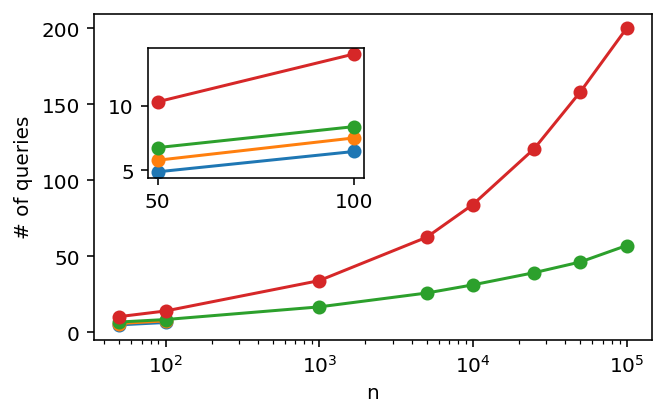
(a) Query complexity

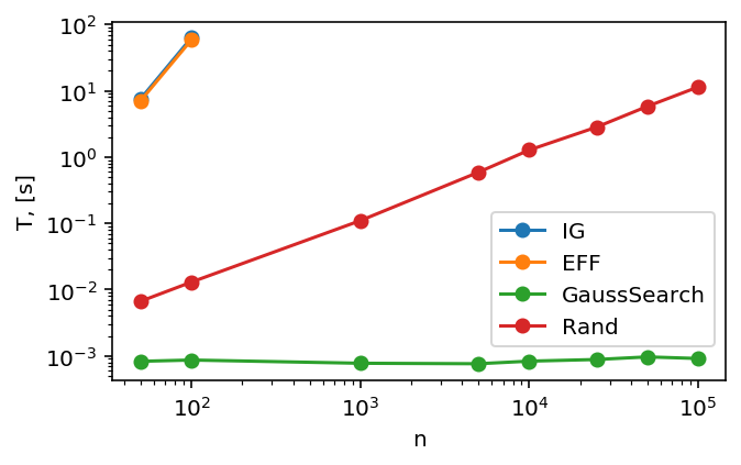
(b) Computational complexity

Figure 1: Average (a) query complexity and (b) computational complexity of four search algorithms in the non-blind setting for $d=5$ and increasing $n$. Search success is declared when $\arg\max_{i\in[n]}P({\bm{x}}_{i})=t$.

The main difference between GaussSearch and previous methods is the way the uncertainty about the target object is modeled. As outlined in Section 2, all previous approaches consider a discrete posterior distribution $P=\{p_{1},p_{2},\dots,p_{n}\}$ over all objects from $[n]$, which is updated after each step using Bayes’ rule. We compared GaussSearch to the baselines that operate on the full discrete distribution and that use different rules to choose the next query: (1) IG: the next query $(i,j)$ is chosen to maximize the expected information gain, (2) Eff: a fast approximation of the EC² active learning algorithm (Golovin et al., 2010) and (3) Rand: the pair of query points is chosen uniformly at random from $[n]$.

In order to assess how well GaussSearch scales in terms of both query and computational complexities in comparison to the other baselines, we run simulations on synthetically generated data of $n$ points uniformly sampled from a $d=5$ dimensional hypercube. We vary the number of points $n$ from 50 to 100000. For each value of $n$, we run 1000 searches, each with a new target sampled independently and uniformly at random among all objects. During the search, comparison outcomes are sampled from the probit model (1), using a value of $\sigma_{\varepsilon}^{2}$ chosen such that approximately 10% of the queries’ outcomes are flipped. In order not to give an undue advantage to our algorithm (which never uses an object in a comparison pair more than once), we change the stopping criterion, and declare that a search is successful as soon as the target $t$ becomes the point with the highest probability mass under a given method’s target model $P$ (ties are broken at random). For the GaussSearch procedure, we take $P({\bm{x}}_{i})$ to be proportional to the density of the Gaussian posterior at ${\bm{x}}_{i}$. We use two performance metrics.

Query complexity

The average number of queries until $\arg\max_{i\in[n]}P({\bm{x}}_{i})=t$, i.e., the true target point has the highest posterior probability.

Computational complexity

The total time needed for an algorithm to decide which query to make next and to update the posterior upon receiving a comparison outcome.

Fig 1a and Fig 1b show the results averaged over 1000 experiments. Both IG and Eff require $O(n^{3})$ operations to choose the next query, as they perform a greedy search over all possible combinations of query pair and target. For these two methods, we report results only for $n=50$ and $n=100$, as the time required for finding the optimal query and updating the posterior for $n>100$ takes over a minute per one step. For $n\in\{50,100\}$, IG performs best in terms of query complexity, with 4.9 and 6.47 queries per search on average for $n=50$ and $n=100$, respectively. However, the running time is prohibitively long already for $n=100$. In constrast, GaussSearch has a favorable tradeoff between query complexity and computational complexity: in comparison to IG, it requires only 1.8 (for $n=50$) or 2 (for $n=100$) additional queries on average, while the running time is improved by several orders of magnitude. We observe that, even though in theory the running time of GaussSearch is not independent of $n$, in practice it is almost constant throughout the range of values of $n$ that we investigate. Finally, we note that Rand performs worst in terms of average number of queries, despite having a higher running time per search step (due to maintaining a discrete posterior).

6.2 Blind Setting

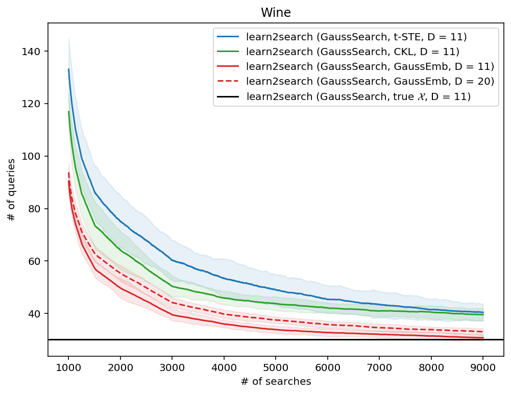
(a)

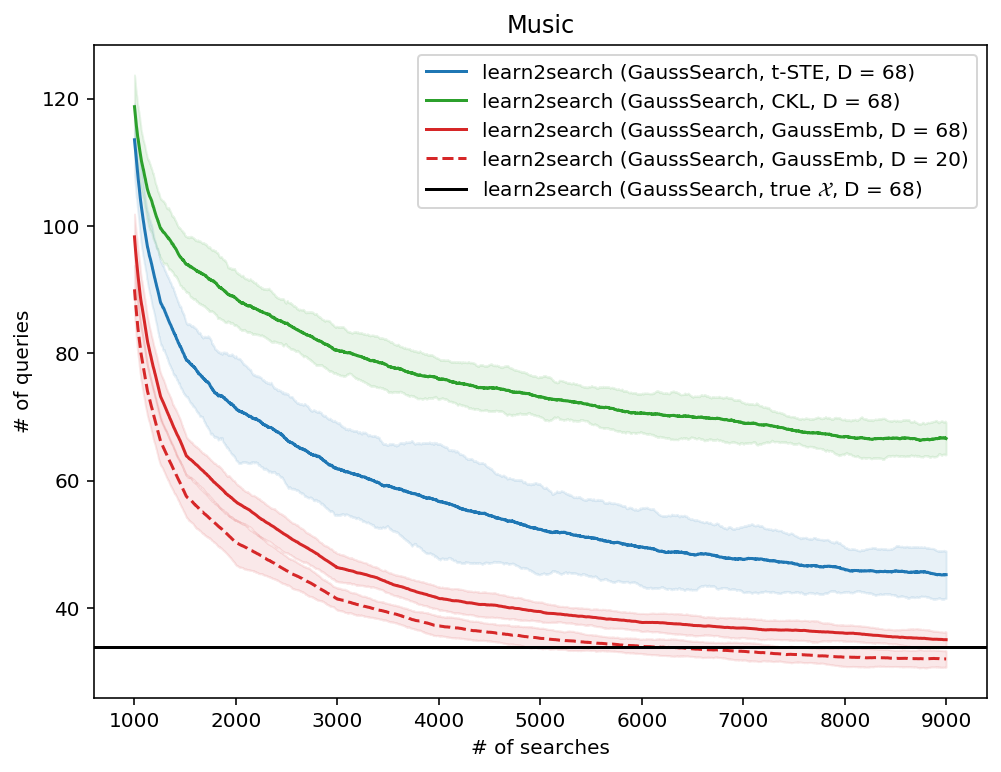
(b)

Figure 2: Combined search and embedding framework learn2search on two datasets with different embedding techniques and choices of $D$. Results are reported over a sliding window of size 1000.

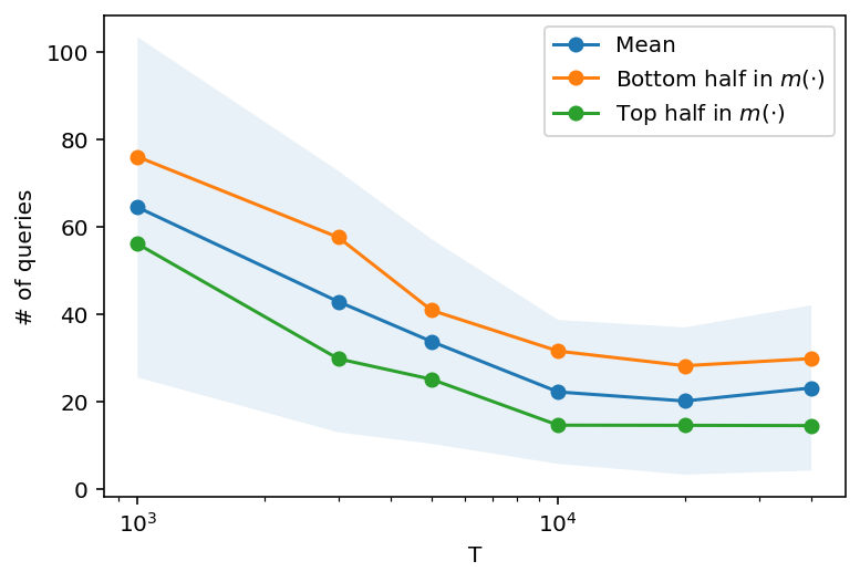
(a)

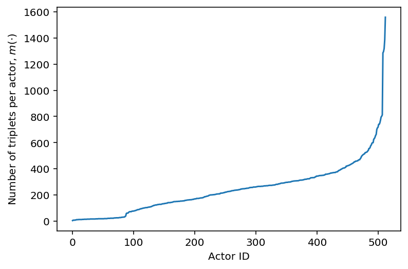
(b)

Figure 3: (a) Empirical search cost, averaged over $5$ human subjects, for a database with $n=513$ faces of movie actors. The averages in the top and bottom group of targets (in terms of number of triplets) are shown individually as well: clearly, the denser group (green) has lower search cost. The blue shaded area shows one std around the average search cost. Note that the $y$-axis is the number of queries (each query features four pictures). Each choice is broken down into 3 pairwise comparison outcomes. (b) Distribution of the number of collected triplets per actor, $m(\cdot)$. The actor with the highest number of triplets is Halle Berry with $m(\mbox{Halle Berry})=1567$ and the actor with the least number of triplets is Kumail Nanjiani with $m(\mbox{Kumail Nanjiani})=16$. The median number of triplets per actor is 227.

We now turn our attention to the blind setting and study the performance of Learn2Search on two real world datasets: the red wine dataset (Cortez et al., 2009) and the music dataset (Zhou et al., 2014). These datasets were studied in the context of comparison-based search by Kazemi et al. (2018). We assume that the feature vectors $\{{\bm{x}}_{1},\ldots,{\bm{x}}_{n}\}$ are latent: they are used to generate comparison outcomes, but they are not available to the search algorithm. We compare different approaches to learning an estimate of the feature vectors from comparison outcomes. In addition to our distributional embedding method GaussEmbed, we consider two state-of-the-art embedding algorithms: $t$-STE (Van Der Maaten & Weinberger, 2012) and CKL (Tamuz et al., 2011) (both of which produce point estimates of the feature vectors), as well as the ground-truth vectors $\mathcal{X}$.

We run 9000 searches in total, starting from a randomly initialized $\hat{\mathcal{X}}$ and updating the embedding on the $k$-th search for $k\in[2^{0},2^{1},\ldots,2^{13}]$ For each search, the target object is chosen uniformly at random among all objects. The outcomes of the comparisons queried by GaussSearch are sampled from the probit model (1) based on the ground-truth feature vectors $\mathcal{X}$. A search episode ends when the target appears as one of the two objects in the query. As before, the noise level $\sigma_{\varepsilon}^{2}$ is set to corrupt approximately 10% of the answers on average. As we jointly perform searches and learn the embedding, we measure the number of queries needed for GaussSearch to find the target using the current version of $\hat{\mathcal{X}}$ for each search, and then we average these numbers over a moving window of size 1000.

We present the results, averaged over 100 experiments, in Fig. 2. The combination of GaussSearch and GaussEmbed manages to learn object representations that give rise to search episodes that are as query-efficient as they would have been using the ground-truth vectors $\mathcal{X}$, and significantly outperforms variants using $t$-STE and CKL for generating embeddings. It appears that taking into account the uncertainty over the points’ locations, as is done by GaussEmbed, helps to make fewer mistakes in early searches and thus leads to a lower query complexity in comparison to using point-estimates of vector embeddings. As the number of searches grows, GaussEmbed learns better and better representations $\hat{\mathcal{X}}$ and enables GaussSearch to ask fewer and fewer queries in order to find the target. In the final stages, our blind search method is as efficient as if it had access to the true embedding on both wine and music datasets.

One of the challenges that arises when learning an embedding in the blind setting is the choice of $D$. In the case when the true $d$ is not known, we estimated it by first conservatively setting $D=100$, and then, after collecting around 10000 triplets, picking the smallest value of $D$ with 98% of the energy in the eigenvalue decomposition of the covariance matrix of the mean vectors $\hat{{\bm{X}}_{\mu}}$. This number for both datasets was $20$, and $D=20$ was used as the approximation of the actual $d$. The results of running our Learn2Search with the estimated $d$ is shown in Fig. 2 as the dashed lines. For the wine dataset, we achieved almost the same query complexity as for true $d$. For the music dataset, after 4000 searches our scheme with estimated $d$ actually outperformed the true features ${\bm{X}}$: on average, when the search is run on $\hat{{\bm{X}}}$, GaussSearch needs fewer queries than when it is performed on ${\bm{X}}$. This suggests that Learn2Search is not only robust to the choice of $D$, but is also capable of learning useful object representations for the comparison-based search independent of the true features of the objects.

6.3 Movie Actors Face Search Experiment

We present the results of an experiment involving human oracles, in order to validate the practical relevance of the model and search algorithm developed in this paper. We collected $n=513$ photographs of the faces of well-known actors and actresses, and we built a web-based search interface implementing the Learn2Search method over this dataset. In this system, a user can look for an actor by comparing faces: at each search iteration, the user is shown $4$ pictures of faces, and can then click on the face that looks the most like the target; this process repeats until the target is among the $4$ samples. Once it is, the user clicks on a button to see details about the target, which ends the search. We have collected slightly more than $40\,000$ comparison triplets from users of the site (which include both project participants as well as outside users, who explored the service out of curiosity). The system is blind, in that we do not extract any explicit features of the faces (shape, eye color, etc.)

We try to answer the following two questions: (i) how efficient are searches? and (ii) how does the search cost depend on the size of the training set? For this, we recruited $5$ subjects, whose task it was to find the face of an actor, which has been sampled uniformly from the $n$ possible targets. For each search, we first sampled $T\in\{1000,3000,5000,10k,20k,40k\}$ triplets, uniformly from the source $40k+$ triplets, and then generated the embedding as described in Section 5. For each value of $T$, each subject performed $10$ searches. The results are shown in Fig. 3a. Observe that for the smallest $T$, the average search cost is essentially equal to the random strategy (which has expected cost $\frac{1}{2}\cdot\frac{n}{4}$). As $T$ increases, the embedding becomes more meaningful, and the search cost drops significantly. In our experiments, the median time-to-answer is around 5 seconds. Thus, once we have ~10k triplets, the time until the target is found is ~2 minutes. We observe small differences in the time-to-answer as a function of the quality of the embedding: with random embeddings, users tend to answer slightly faster (probably because the images are very different to the target).

An additional comment on the variance in search cost is in order. Call $m(i)$ the number of triplets in $T$ that object $i$ is part of (in any position). In our full experimental dataset, $m(i)$ is heavily skewed, see Fig. 3b, because (a) objects were added to the system gradually over time, and (b) the distribution over targets follows popularity, which is heavily skewed itself. Concretely, this ranges from $m(\mbox{Halle Berry})=1567$ to $m(\mbox{Kumail Nanjiani})=16$. It is natural to suspect that a target $t$ with larger $m(t)$ is easier to find, because its embedding is more precise relative to other objects. Indeed, our results bear this out: in Fig. 3a, we break out the search cost for the top and bottom half of targets separately. This suggests that if we could collect further data, including for the sparse targets (low $m(t)$), the asymptotic search cost would be reduced further. In summary, our experiment shows that Learn2Search is able to extract an embedding in the blind setting that appears to align with visual features that human oracles rely on to find a face, and is able to navigate through this embedding to locate a target efficiently.

7 Conclusion

In this work, we introduce a probablistic model of triplet comparisons, a search algorithm for finding a target among a set of alternatives, and a Bayesian embedding algorithm for triplet data. Our search algorithm is backed by theoretical guarantees and strikes a favorable computational vs. query complexity trade-off. By combining the search and embedding algorithms, we design a system that learns to search efficiently without a-priori access to object features. We observe that the search cost successfully decreases as the number of search episodes increases. This is achieved by iteratively refining a distributional, latent, and low-dimensional representation of the objects. Our framework is scalable in the number of objects $n$, tolerates noisy answers, and performs well on synthetic and real-world experiments.

Appendix A Supplementary Material

This supplementary material contains:

1. Proofs of Theorem 1 and Theorem 2.

2. Additional experiments on comparing different embedding techniques.

3. Additional plot of the 2-PCA of the learned embedding in the movie actors face search experiment.

Appendix B Proof of Theorem 1

Proof.

Without loss of generality, assume that $\sigma_{\varepsilon}=1$. Let $y$ be a binary random variable such that $p(y=1|{\bm{w}},b,{\bm{x}})=\Phi({\bm{x}}^{T}{\bm{w}}+b)$. Then,

$$\operatorname*{arg\,max}_{({\bm{w}},b)\in\mathcal{H}}I[{\bm{x}};y\mid({\bm{w}},b)]$$

$$\quad=\operatorname*{arg\,max}_{({\bm{w}},b)\in\mathcal{H}}\left\{1-\mathbb{E}_{\hat{{\bm{x}}}}[H(y\mid{\bm{w}},b,{\bm{x}})]\right\}$$ (4)

$$\quad=\operatorname*{arg\,min}_{({\bm{w}},b)\in\mathcal{H}}\int_{\mathbb{R}^{d}}H\left[\Phi({\bm{x}}^{T}{\bm{w}}+b)\right]\mathcal{N}({\bm{x}};{\bm{\mu}},{\bm{\Sigma}})d{\bm{x}}$$

$$\quad=\operatorname*{arg\,min}_{({\bm{w}},b)\in\mathcal{H}}\int_{\mathbb{R}}H\left[\Phi(t)\right]\mathcal{N}(t;0,{\bm{w}}^{T}{\bm{\Sigma}}{\bm{w}})dt$$ (5)

$$\quad=\operatorname*{arg\,max}_{({\bm{w}},b)\in\mathcal{H}}{\bm{w}}^{T}{\bm{\Sigma}}{\bm{w}}.$$ (6)

In (4), we use (2) and the fact that, as the hyperplane is passing through ${\bm{\mu}}$,

$$H\left[\int_{\mathbb{R}^{d}}p(y=1|{\bm{w}},b,{\bm{x}})\mathcal{N}({\bm{x}};{\bm{\mu}},{\bm{\Sigma}})d{\bm{x}}\right]=H(1/2)=1.$$

In (5), we use the fact that ${\bm{x}}^{T}{\bm{w}}+b\sim\mathcal{N}(\bm{0},{\bm{w}}^{T}{\bm{\Sigma}}{\bm{w}})$, by properties of the Gaussian distribution. Finally, in (6), we start by noting that, for all $c_{1},c_{2}$ such that $c_{1}/c_{2}>1$, $H\left[\Phi(c_{1}t)\right]\leq H\left[\Phi(c_{2}t)\right]$ for all $t$ with equality iff $t=0$. Hence, if $\tilde{\sigma}^{2}>\sigma^{2}$, then

$$\int_{\mathbb{R}}H\left[\Phi(t)\right]\mathcal{N}(t;0,\tilde{\sigma}^{2})dt=\int_{\mathbb{R}}H\left[\Phi(\tilde{\sigma}t)\right]\mathcal{N}(t;0,1)dt$$

$$<\int_{\mathbb{R}}H\left[\Phi(\sigma t)\right]\mathcal{N}(t;0,1)dt=\int_{\mathbb{R}}H\left[\Phi(t)\right]\mathcal{N}(t;0,\sigma^{2})dt.$$

Therefore, maximizing ${\bm{w}}^{T}{\bm{\Sigma}}{\bm{w}}$ minimizes the expected entropy of $y$. ∎

Appendix C Proof of Theorem 2

For simplicity, we will assume that $d=1$; Section C.1 explains how to generalize the result to any $d>1$. Denote by $x_{t}$ the location of the target object, and let $\mathcal{N}(\hat{x};\mu_{m},\sigma_{m})$ be the belief about the target’s location after $m$ observations. Without loss of generality, let $\sigma_{\varepsilon}^{2}=1$. In this case, the updates have the following form.

$$\sigma^{2}_{m+1} =\sigma^{2}_{m}+\beta_{m}\sigma^{4}_{m},$$ (7)

$$\mu_{m+1} =\mu_{m}+\alpha_{m}\sigma^{2}_{m}\cdot z_{m},$$

where $z_{m}\in\{\pm 1\}$ with $\mathbf{P}(z_{m}=1)=\Phi(x_{t}-\mu_{m})$, and

$$\alpha_{m} =c/\sqrt{\sigma_{m}^{2}+1},$$

$$\beta_{m} =-c^{2}/(\sigma_{m}^{2}+1),$$

$$c =\sqrt{2/\pi}.$$

We start with a lemma that essentially states that $\sigma_{m}^{2}$ decreases as $1/m$.

Lemma 1.

For any initial $\sigma_{0}^{2}>0$ and for all $m\geq 0$, the posterior variance $\sigma_{m}^{2}$ can be bounded as

$$\frac{\min\{0.1,\sigma_{0}^{2}\}}{m+1}\leq\sigma_{m}^{2}\leq\frac{\max\{10,\sigma_{0}^{2}\}}{m+1}.$$

Proof.

From (7), we know that

$$\sigma_{m+1}^{2}=\left(1-c^{2}\frac{\sigma_{m}^{2}}{\sigma_{m}^{2}+1}\right)\sigma_{m}^{2}$$

First, we need to show that

$$f(x)=\left(1-c^{2}\frac{x}{x+1}\right)x$$

is increasing on $\mathbf{R}_{>0}$. This is easily verified by checking that

$$f^{\prime}(x)=\left(1-c^{2}\frac{x}{x+1}\right)+x\left(1-c^{2}\frac{1}{(x+1)^{2}}\right)\geq 0,$$

for all $x\in\mathbf{R}_{>0}$ Next, we consider the upper bound. Let $b=\max\{10,\sigma_{0}^{2}\}$. We will show that $\sigma_{m}^{2}\leq b/(m+1)$ by induction. The basis step is immediate: by definition, $\sigma_{0}^{2}\leq b$. The induction step is as follows, for $m\geq 1$.

$$\sigma_{m}^{2}=\left(1-c^{2}\frac{\sigma_{m-1}^{2}}{\sigma_{m-1}^{2}+1}\right)\sigma_{m-1}^{2}$$

$$\qquad\leq\left(1-c^{2}\frac{b}{b+m}\right)\frac{b}{m}\leq\frac{b}{m+1}$$

$$\iff 1-c^{2}\frac{b}{b+m}-\frac{m}{m+1}\leq 0$$

$$\iff b+m-c^{2}(bm+b)\leq 0$$

$$\iff m(1-c^{2}b)+b(1-c^{2})\leq 1-b(\underbrace{2c^{2}-1}_{\approx 0.27})\leq 0,$$

where the first inequality holds because $f(x)$ is increasing. The lower bound can be proved in a similar way. ∎

For completeness, we restate Theorem 2 for $d=1$.

Theorem 2 (Case $d=1$).

If the answers follow equation 1, then for any initial $\mu_{0}$ and $\sigma_{0}^{2}>0$ and as $m\to\infty$,

$$\sigma_{m}^{2} \to 0,$$

$$\mu_{m} \to x_{t}$$

almost surely.

Proof.

The first part of the theorem ($\sigma_{m}^{2}\to 0$) is a trivial consequence of Lemma 1. The second part follows from the fact that our update procedure can be cast as the Robbins-Monro algorithm (Robbins & Monro, 1951) applied to $g(\mu)\doteq 2\Phi(x_{t}-\mu)-1$, which has a unique root in $\mu=x_{t}$. Indeed, $z_{m}$ is a stochastic estimate of the function $g$ at $\mu_{m}$, i.e., $\mathbf{E}(z_{m})=2\Phi(\mu_{m}-x_{t})-1$. The remaining conditions to check are as follows.

• the learning rate $\gamma_{m}=\alpha_{m}\sigma_{m}^{2}$ satisfies

  $$\sum_{m=0}^{\infty}\gamma_{m} \geq\frac{c\cdot\min\{\sigma_{0}^{2},0.1\}}{\sqrt{\sigma_{0}^{2}+1}}\sum_{m}^{\infty}\frac{1}{m}=\infty,$$

  $$\sum_{m=0}^{\infty}\gamma_{m}^{2} \leq(c\cdot\max\{\sigma_{0}^{2},10.0\})^{2}\sum_{m}^{\infty}\frac{1}{m^{2}}<\infty$$

• $\lvert z_{m}\rvert\leq 1$ for all $m$

Almost sure convergence then follows directly from the results derived in (Robbins & Monro, 1951) and (Blum et al., 1954). ∎

C.1 Extending the proof to $d>1$

In order to understand how to extend the argument of the proof given above to $d>1$, the following observation is key: Every query made during a search gives information on the position of the target along a single dimension, i.e., the one perpendicular to the bisecting hyperplane. This can be seen, e.g., from the update rule

$${\bm{\Sigma}}_{m+1} =\left({\bm{\Sigma}}_{m}+\tau{\bm{w}}_{i_{m},j_{m}}\otimes{\bm{w}}_{i_{m},j_{m}}^{T}\right)^{-1},$$

which reveals that the precision matrix (i.e., the inverse of the covariance matrix) is affected only in the subspace spanned by ${\bm{w}}_{i_{m},j_{m}}$.

Therefore, if we start with $\bm{\Sigma}_{0}=\sigma_{0}^{2}\bm{I}$, we can (without loss of generality) assume that the search procedure sequentially iterates over the dimensions. At each iteration, the variance shrinks along that dimension only, leaving the other dimensions untouched. Conceptually, we can think of the case $d>1$ as interleaving $d$ independent one-dimensional search procedures. Each of these one-dimensional searches converges to the corresponding coordinate of the target vector $\bm{x}_{t}$, and the variance along the corresponding dimension shrinks to $0$.

In general, one should consider the fact that the optimal hyperplane is not always unique, and the chosen hyperplane might not align with the current basis of the space. This case can be taken care of by re-parametrizing the space by using a rotation matrix. However, these technical details do not bring any new insight as to why the result holds.

Appendix D Performance of Embedding Methods

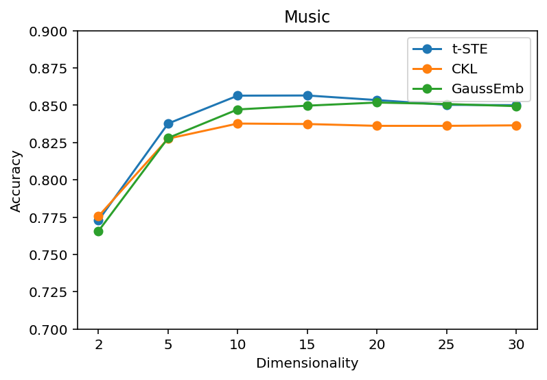
(a)

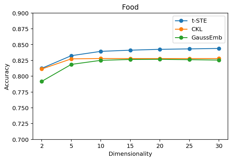
(b)

Figure 4: Evaluating embedding methods on two real world datasets: Music artists, $n=400$ music artists with $9090$ triplet comparisons after removing repeating and inconsistent triplets, and Food, $n=100$ images of food with $190376$ collected unique triplets.

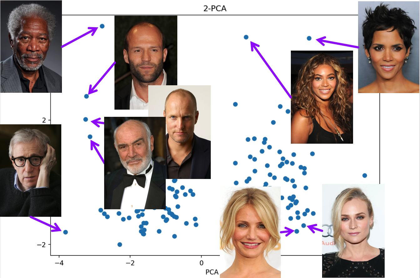
Figure 5: 2-PCA on learned embedding.

We evaluated the quality of the object embedding learned by our embedding technique GaussEmb on two real world datasets with crowdsourced triplet comparisons: Music artists (Ellis et al., 2002) and Food (Wilber et al., 2014).

We compared our model to the state-of-the-art baselines, CKL and t-STE. We measured accuracy—the percentage of satisfied triplets in the learned embeddings on a holdout set using 10-fold cross validation. Since the “true” dimensionality of the feature space is not known a priori, we also vary the dimensionality $D$ of the estimated embedding between 2 and 30. The results are presented in Fig. 4.

Overall, on both datasets, GaussEmb showed similar performance to t-STE, correctly modeling between 83% and 85% of triplets, and outperformed CKL. We can conclude that the noise model considered in this paper reflects the real user behaviour on the comparison-like tasks well.

Appendix E Movie Actors Face Search Experiment

We illustrate the results of performing 2-PCA on the learned embedding from the movie actors face search experiment in Fig. 5. It appears that the two principal components align well with gender and race. Note that this embedding was obtained solely from the triplet comparisons collected prior to the experiment (slightly more than 40000 triplets in total).

References

- Agarwal et al. (2007) Agarwal, S., Wills, J., Cayton, L., Lanckriet, G., Kriegman, D., and Belongie, S. Generalized non-metric multidimensional scaling. In Artificial Intelligence and Statistics, pp. 11–18, 2007.
- Amid & Ukkonen (2015) Amid, E. and Ukkonen, A. Multiview triplet embedding: Learning attributes in multiple maps. In International Conference on Machine Learning, pp. 1472–1480, 2015.
- Anderton & Aslam (2019) Anderton, J. and Aslam, J. Scaling up ordinal embedding: A landmark approach. In International Conference on Machine Learning, pp. 282–290, 2019.
- Bentley (1975) Bentley, J. L. Multidimensional binary search trees used for associative searching. Communications of the ACM, 18(9):509–517, 1975.
- Blum et al. (1954) Blum, J. R. et al. Approximation methods which converge with probability one. The Annals of Mathematical Statistics, 25(2):382–386, 1954.
- Bradley & Terry (1952) Bradley, R. A. and Terry, M. E. Rank analysis of incomplete block designs: I. The method of paired comparisons. Biometrika, 39(3/4):324–345, 1952.
- Brochu et al. (2008) Brochu, E., de Freitas, N., and Ghosh, A. Active preference learning with discrete choice data. In Advances in neural information processing systems, pp. 409–416, 2008.
- Canal et al. (2019) Canal, G., Massimino, A., Davenport, M., and Rozell, C. Active embedding search via noisy paired comparisons. In Proceedings of the 36th International Conference on Machine Learning (ICML), 2019.
- Chang & Tsao (2017) Chang, L. and Tsao, D. Y. The code for facial identity in the primate brain. Cell, 169(6):1013–1028, 2017.
- Chu & Ghahramani (2005) Chu, W. and Ghahramani, Z. Extensions of Gaussian processes for ranking: Semi-supervised and active learning. In Proceedings of the NIPS 2005 Workshop on Learning to Rank, Whistler, BC, Canada, December 2005.
- Cortez et al. (2009) Cortez, P., Cerdeira, A., Almeida, F., Matos, T., and Reis, J. Modeling wine preferences by data mining from physicochemical properties. Decision Support Systems, 47(4):547–553, 2009.
- Cox et al. (2000) Cox, I. J., Miller, M. L., Minka, T. P., Papathomas, T. V., and Yianilos, P. N. The bayesian image retrieval system, pichunter: theory, implementation, and psychophysical experiments. IEEE transactions on image processing, 9(1):20–37, 2000.
- Dasgupta (2005) Dasgupta, S. Analysis of a greedy active learning strategy. In Advances in neural information processing systems, pp. 337–344, 2005.
- Datta et al. (2008) Datta, R., Joshi, D., Li, J., and Wang, J. Z. Image retrieval: Ideas, influences, and trends of the new age. ACM Computing Surveys (Csur), 40(2):5, 2008.
- Ellis et al. (2002) Ellis, D. P., Whitman, B., Berenzweig, A., and Lawrence, S. The quest for ground truth in musical artist similarity. In ISMIR. Paris, France, 2002.
- Fang & Geman (2005) Fang, Y. and Geman, D. Experiments in mental face retrieval. In International Conference on Audio-and Video-Based Biometric Person Authentication, pp. 637–646. Springer, 2005.
- Ferecatu & Geman (2009) Ferecatu, M. and Geman, D. A statistical framework for image category search from a mental picture. IEEE Transactions on Pattern Analysis and Machine Intelligence, 31(6):1087–1101, 2009.
- Ghosh et al. (2019) Ghosh, N., Chen, Y., and Yue, Y. Landmark ordinal embedding. In Advances in Neural Information Processing Systems, pp. 11506–11515, 2019.
- Golovin et al. (2010) Golovin, D., Krause, A., and Ray, D. Near-optimal bayesian active learning with noisy observations. In Advances in Neural Information Processing Systems, pp. 766–774, 2010.
- Haghiri et al. (2017) Haghiri, S., Ghoshdastidar, D., and von Luxburg, U. Comparison-based nearest neighbor search. In Artificial Intelligence and Statistics, pp. 851–859, 2017.
- Heim et al. (2015) Heim, E., Berger, M., Seversky, L. M., and Hauskrecht, M. Efficient online relative comparison kernel learning. In Proceedings of the 2015 SIAM International Conference on Data Mining, pp. 271–279. SIAM, 2015.
- Houlsby et al. (2011) Houlsby, N., Huszár, F., Ghahramani, Z., and Lengyel, M. Bayesian active learning for classification and preference learning. arXiv preprint arXiv:1112.5745, 2011.
- Jain et al. (2016) Jain, L., Jamieson, K. G., and Nowak, R. Finite sample prediction and recovery bounds for ordinal embedding. In Advances In Neural Information Processing Systems, pp. 2711–2719, 2016.
- Jamieson & Nowak (2011) Jamieson, K. G. and Nowak, R. D. Low-dimensional embedding using adaptively selected ordinal data. In Communication, Control, and Computing (Allerton), 2011 49th Annual Allerton Conference on, pp. 1077–1084. IEEE, 2011.
- Karbasi et al. (2012) Karbasi, A., Ioannidis, S., and Massoulié, L. Comparison-based learning with rank nets. In Proceedings of the 29th International Conference on Machine Learning (ICML), 2012.
- Kazemi et al. (2018) Kazemi, E., Chen, L., Dasgupta, S., and Karbasi, A. Comparison based learning from weak oracles. In International Conference on Artificial Intelligence and Statistics, pp. 1849–1858, 2018.
- Kingma & Welling (2014) Kingma, D. P. and Welling, M. Auto-encoding variational Bayes. In Proceedings of ICLR 2014, Banff, AB, Canada, April 2014.
- Kleindessner & von Luxburg (2017) Kleindessner, M. and von Luxburg, U. Kernel functions based on triplet comparisons. In Advances in Neural Information Processing Systems, pp. 6807–6817, 2017.
- MacKay (1992) MacKay, D. J. Information-based objective functions for active data selection. Neural computation, 4(4):590–604, 1992.
- Minka (2001) Minka, T. P. A family of algorithms for approximate Bayesian inference. PhD thesis, Massachusetts Institute of Technology, 2001.
- Nowak (2008) Nowak, R. Generalized binary search. In Communication, Control, and Computing, 2008 46th Annual Allerton Conference on, pp. 568–574. IEEE, 2008.
- Nowak (2009) Nowak, R. Noisy generalized binary search. In Advances in neural information processing systems, pp. 1366–1374, 2009.
- Rezende et al. (2014) Rezende, D. J., Mohamed, S., and Wierstra, D. Stochastic backpropagation and approximate inference in deep generative models. In International Conference on Machine Learning, pp. 1278–1286, 2014.
- Robbins & Monro (1951) Robbins, H. and Monro, S. A stochastic approximation method. The annals of mathematical statistics, 22(3):400–407, 1951.
- Settles (2012) Settles, B. Active Learning. Morgan & Claypool Publishers, 2012.
- Suditu & Fleuret (2012) Suditu, N. and Fleuret, F. Iterative relevance feedback with adaptive exploration/exploitation trade-off. In Proceedings of the 21st ACM International Conference on Information and Knowledge Management, pp. 1323–1331. ACM, 2012.
- Sun et al. (2012) Sun, Z., Wang, H., Wang, H., Shao, B., and Li, J. Efficient subgraph matching on billion node graphs. Proceedings of the VLDB Endowment, 5(9):788–799, 2012.
- Tamuz et al. (2011) Tamuz, O., Liu, C., Belongie, S., Shamir, O., and Kalai, A. T. Adaptively learning the crowd kernel. In Proceedings of the 28th International Conference on Machine Learning (ICML), pp. 673–680. Omnipress, 2011.
- Thurstone (1927) Thurstone, L. L. A law of comparative judgment. Psychological Review, 34(4):273–286, 1927.
- Tschopp et al. (2011) Tschopp, D., Diggavi, S., Delgosha, P., and Mohajer, S. Randomized algorithms for comparison-based search. In Advances in Neural Information Processing Systems, pp. 2231–2239, 2011.
- Van Der Maaten & Weinberger (2012) Van Der Maaten, L. and Weinberger, K. Stochastic triplet embedding. In Machine Learning for Signal Processing (MLSP), 2012 IEEE International Workshop on, pp. 1–6. IEEE, 2012.
- Wilber et al. (2014) Wilber, M. J., Kwak, I. S., and Belongie, S. J. Cost-effective hits for relative similarity comparisons. In Second AAAI conference on human computation and crowdsourcing, 2014.
- Zhou et al. (2014) Zhou, F., Claire, Q., and King, R. D. Predicting the geographical origin of music. In 2014 IEEE international conference on data mining (ICDM), pp. 1115–1120. IEEE, 2014.