Investigation of two photon emission in strong field QED using channeling
in a crystal
Tobias N. Wistisen
Max-Planck-Institut für Kernphysik, Saupfercheckweg 1, D-69117, Germany
Abstract
We investigate the 2nd order process of two photons being emitted
by a high-energy electron dressed in the strong background electric
field found between the planes in a crystal. The strong crystalline
field combined with ultra relativistic electrons is one of very few
cases where the Schwinger field can be experimentally achieved in
the electron’s rest frame. The radiation being emitted, the so-called
channeling radiation, is a well studied phenomenon. However only the
first order diagram corresponding to emission of a single photon has
been studied so far. We elaborate on how the 2 photon emission process
should be understood in terms of a two-step versus a one-step process,
i.e., if one can consider one photon being emitted after the other,
or if there is also a contribution where the two photons are emitted
’simultaneously’. From the calculated full probability we see that
the two-step contribution is simply the product of probabilities for
single photon emission while the additional one-step terms are, mainly,
interferences due to several possible intermediate virtual states.
These terms can contribute significantly when the crystal is thin.
Therefore, in addition, we see how one can, for a thick crystal, calculate
multiple photon emissions quickly by neglecting the one-step terms,
which represents a solution of the problem of quantum radiation reaction
in a crystal beyond the usually applied constant field approximation.
We explicitly calculate an example of 180 GeV electrons in a thin
Silicon crystal and argue why it is, for experimental reasons, more
feasible to see the one-step contribution in a crystal experiment
than in a laser experiment.
Strong field QED is the study of physical processes that take place
in a strong background field and nonlinear effects of quantum nature
arise when the size of the Lorentz invariant parameter
(1)
is on the order of unity, which is the ratio of the electromagnetic
field experienced in the electron’s rest frame compared to the Schwinger
field strength . Here
is the elementary charge, the electron mass,
the electromagnetic field tensor of the background field and
the electron 4-momentum. We use natural units such that ,
. Lindhard was one of the first to realize that when
high energy charged particles are aimed close to the direction along
an axis or plane in a crystal, the charged particle can become transversely
trapped Lindhard (1965). Later it was studied how this motion leads
to radiation emission called channeling radiation, especially relevant
for electrons and positrons. This is well-studied both experimentally
Bak et al. (1985, 1988); Swent et al. (1979); Andersen et al. (1981, 1982); Klein et al. (1985); Alguard et al. (1979); Andersen et al. (2012); Uggerhøj (2005)
and theoretically Kumakhov (1976, 1977); Andersen et al. (1981); Sáenz et al. (1981); Kimball and Cue (1985).
Crystal channeling represents one of the only phenomena where the
Schwinger field can be experimentally achieved in the electron’s rest
frame Belkacem et al. (1986); Andersen et al. (1982); Esberg et al. (2010); Wistisen et al. (2018),
with the only other example being the famous E-144 SLAC experiment
on non lienar Compton scattering Bula et al. (1996) using
relativistic electrons colliding with a laser beam. Crystals with
ultra relativistic electrons or positrons therefore present a unique
possibility to study physics in such strong fields. However a calculation
from first principles of emission of more than 1 photon has not been
carried out for crystal channeling. The recent studies of 2 photon
emission in the collision of relativistic electrons with a laser pulse
Seipt and Kämpfer (2012); Mackenroth and Di Piazza (2013); Dinu and Torgrimsson (2018a); King (2015)
show that the emission of 2 photons is not exactly the product of
probabilities for each emission, however under certain conditions
it is an acceptable approximation. The experimental verification of
such results are however complicated in the case of the laser pulse
colliding with an electron bunch because any two (or more) emitted
photons cannot be known to be emitted by the same electron. In crystal
experiments as in e.g. Wistisen et al. (2018), it is standard
that each incoming particle is recorded as a separate event, and therefore
the measured outgoing photons are sure to stem from the single incoming
particle. Therefore, in this paper, we will calculate the emission
of 2 photons during electron channeling in a crystal, which could
potentially be studied experimentally in an experiment similar to
the one seen in Wistisen et al. (2018), however with a modified
setup to allow for the detection of an additional photon. For the
theory of channeling radiation, in particular the development of the
semi-classical operator method by Baier et. al. Baier and Katkov (1968)
stands out, and has been extensively applied to the phenomenon of
channeling Baier et al. (1998).
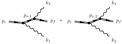
Figure 1: The Feynman diagrams corresponding to the process under study. The
double fermion lines correspond to positron solutions of the Dirac
equation in the background field of the inter planar crystal potential.
This method allowed to include quantum effects such as the electron
spin and the photon recoil, which are important when is no
longer small, while needing only the classical trajectory of the electron/positron
in the external field. The authors of this method, seeking analytical
results, in most applications to channeling, applied the approximation
of the local constant field which greatly simplifies calculations.
The constant field approximation means that while a particle moves
in an external field, which is not constant, one applies the result
of the constant field formula locally, i.e. in a small time step.
Effectively this means neglecting that the radiation emitted before
or after can interfere with this radiation. This is valid only for
certain parameters of fields and particle energies. However the semi-classical
operator method can be used to calculate the radiation emission under
general circumstances without much effort, also when the constant
field approximation is no longer valid Wistisen (2014, 2015),
which with modern computing power makes it one of the most powerful
methods to calculate the radiation emitted by ultra-relativistic electrons
in a general field configuration. There are caveats however, which
are two-fold. Firstly, the notion of a classical trajectory should
make sense. Or, in other words, the quantum numbers associated with
the motion should be large, a subject recently studied in Wistisen and Di Piazza (2019, 2018).
Secondly, the derivation starts out from the first-order diagram of
a dressed electron emitting a single photon. Therefore the emission
rate of two, or more, photons can not be predicted by this method
without approximations. The emission of a single photon yields a rate,
an emission probability per unit time, and as such one can construct
the probability for emitting several photons by applying this rate
for each consecutive emission. In this way, the probability to emit,
e.g., two photons would be proportional to time, or thickness of the
crystal, squared, and so on. We will call this process the ’cascade’
process. Herein lies an approximation, where interference between
different emissions is neglected. We show that the two-photon emission
probability contains the cascade along with one-step terms which scale
linearly with the crystal thickness. Therefore, for sufficiently thin
crystals, these one-step terms will become important. This phenomenon
is also discussed in pair production of electron/positron pairs from
high energy photons in a strong field where one also distinguishes
between the two-step and the one-step, or ’trident’ process. This
has been investigated in crystals in Esberg et al. (2010) and has received
renewed interest with the prospect of studying such phenomena in high-intensity
laser fields Hu et al. (2010); Ilderton (2011); Acosta and Kämpfer (2019); King and Fedotov (2018); Dinu and Torgrimsson (2018b); Mackenroth and Di Piazza (2018).
In this paper we make quantitative calculations of the angularly integrated
probability, differential in photon energies, of emission of two photons
by an electron in the planar Doyle-Turner potential Baier et al. (1998); Doyle and Turner (1968); Avakian et al. (1982); Møller (1995).
We do this by finding numerical solutions of the Dirac equation by
solving the problem in a basis of plane waves, which is possible due
to the periodicity of the transverse potential in a crystal, as shown
in Wistisen and Di Piazza (2019). If the cascade terms are enough to properly
describe the radiation emission is a highly relevant question as it
closely relates to the phenomenon of quantum radiation reaction, the
emission of multiple photons when is large, Di Piazza et al. (2010),
recently studied using channeling radiation and in laser experiments
Wistisen et al. (2018); Poder et al. (2018); Cole et al. (2018).
In the crystal experiment it was seen that even for energies as high
as GeV positrons, where it could be expected that the constant
field approximation would be acceptable, it was shown that discrepancies
arise due to this, and therefore a more general theory was called
for. The current theory of quantum radiation reaction in lasers relies
on the local constant field approximation Di Piazza et al. (2010); Neitz and Di Piazza (2013); Blackburn et al. (2014); Baier et al. (1998); Vranic et al. (2016); Li et al. (2014),
and it is unknown if one can calculate the emission of many photons
in a way that avoids calculating all the corresponding higher order
diagrams, when going beyond the constant field approximation. This
question will be addressed in the case of a crystal, in the current
paper.
We use the Feynman slash notation such that , where are the Dirac gamma matrices and an arbitrary four-vector. We adopt the metric tensor .
I Formalism
In QED the transition amplitude from a given initial state
to a final state is given by
(2)
where is the time evolution operator, often written as
where is the time-ordering operator and
is the quantized interaction. We then write our quantized fields as
(3)
(4)
where and are an orthonormal
and complete set of electron and positron solutions, respectively,
in the background field. denotes
a summation over all states, and the relevant quantum numbers
which we will find later. The , and operators are the
annihilation operators of the electron, positron and photon field
respectively, obeying the relations, that the only non-zero (anti-)commutators
are ,
where the brackets denote the anti-commutator and the
commutator.
In Wistisen and Di Piazza (2019, 2018) we discussed the Dirac
equation with the potential found in the crystal, but we will here
repeat the results we need in order to calculate the emission of 2
photons. It was found in Wistisen and Di Piazza (2019) that the electron solution
can be written as follows
(5)
and the positron solutions can then be written as (see appendix A)
and and are given by
where ,
is the electrostatic potential, is the charge,
the superscript on refers to the charge sign,
is a two component vector describing the spin, which we can choose
as either or , corresponding to spin-up and spin-down respectively for the electron,
and opposite for the positron. From the choice of the form of the
spinors and , it is also clear that positive
should be used (see appendix A). is the solution
to the equation
(6)
For we will use the Doyle-Turner model Baier et al. (1998); Doyle and Turner (1968); Avakian et al. (1982); Møller (1995),
chosen as symmetric around 0. In a crystal this potential
is periodic with the period of the inter planar distance which we
will denote as . Because of this, the solution (for the electron)
can be written as a Bloch wave such that
(7)
and where is also periodic with period
and is the Bloch momentum, which can be taken to be in
the interval , .
It then follows from Blochs theorem that these solutions form an orthogonal
and complete set of solutions of Eq. (6). Inserting
of Eq. (7) into Eq. (6)
gives us the equation governing
(8)
The periodicity of means it can be written as a Fourier
series,
(9)
To ensure normalization we should have
(see appendix B). It is now clear that this is an eigenvalue
problem for each where the quantized eigenvalue is
(10)
where is the quantum number corresponding to the value of this
energy in ascending order and where is the ground state. This
equation leads to a quantization of e.g. . The coefficients
are found by solving the matrix eigenvalue problem obtained
by inserting Eq. (9) in Eq. (8)
and multiply with and integrate over
from to to exploit orthogonality
(11)
This was done with the electron function in mind, but
the positron coefficients can be obtained just by changing . With
these things taken into consideration, we now see that we can write
the and functions in terms of the coefficients
such that
(12)
(13)
where
(14)
(15)
where .
For the calculation of radiation emission from electrons we will need
the quantity ,
where we have put labels for the initial state and final state
, however these still each depend on the index . This quantity
can then be written as
(16)
where
(17)
(18)
Now since we have an orthonormal complete set of solutions, we can
write the propagator in terms of these states as Beresteckij et al. (2008)
This expression can be simplified due to the simple expression for
the wave functions in all coordinates but the coordinate. However,
we will not carry this out, as it is easier to see how the cascade
part of the radiation emission arises by starting from the above expression.
II Single photon emission and cascade
We will now briefly mention some results obtained in Wistisen and Di Piazza (2019)
on the single photon emission probability which is relevant to build
the expected cascade contribution. We found that the rate of emission
is given by
(19)
where we defined
(20)
where is the integer such that , where
, corresponds
to the initial state and is coefficient with index
corresponding to the initial state . See the appendix
of Wistisen and Di Piazza (2019) for the details on why reduces
to a single sum over . As shown in Wistisen and Di Piazza (2019) there
are large terms in which
cancel, leaving behind the relevant small terms, because the relevant
transverse energies , comparable to the potential depth, are
much smaller than the whole particle energy i.e. eV versus GeV. We
could rewrite the content of the delta function as
(21)
Now we may use that
where is the positive solution to . From
the formula for single photon emission, Eq. (19),
we can construct the cascade contribution to two photon emission.
We wish to know the probability of finding a photon in the momentum
interval around while also finding a photon
within another interval around . This can happen
in two ways, either the particle emits while transitioning
from the initial state, and then subsequently or vice versa.
We are however interested in the angular integrated spectrum, that
is
and therefore an additional factor of must be added
due to counting the same point in phase space twice Feynman (1965),
and so we obtain
(22)
III Two photon emission
Expanding the time evolution operator to second order, allowing for
two photon emission we have that the S-matrix element is
(23)
When specifying the final state as ,
an electron and two photons and the initial state as just an electron,
, can be rewritten
in terms of the wave functions and the propagator. In Beresteckij et al. (2008)
this is done for the Compton scattering matrix element, which is the
same diagram as here, except that an incoming photon is instead outgoing.
The matrix element is therefore
(24)
Now we define
(25)
where is defined as in Eq. (20) where
is used to denote the virtual state from the propagator, and
is shorthand for the dependence on , , ,
and . The superscript on and
denotes that the virtual state is the electron state ,
and , is the same but with the positron
virtual state. The matrix element may then be written as
(26)
Therefore the term in the second line is seen as the electron first
emits a photon with momentum at and
then propagates to a later time and emits a second photon
with momentum . The term in the third line is
then the electron emitting the photon with momentum
at a time turning the electron into a positron going into
the past and emitting the photon with momentum
at the earlier time . This last term is heavily suppressed
in our case which we can see as follows. Denote
and , then we may use
that
(27)
where is a small real number for which one in the end
should take the limit and therefore we have
(28)
We have also that
and therefore we have the term from the third line of Eq. (26)
carries the factor of
(29)
and therefore this term will always be very far off-shell, as the
virtual particle on-shell condition can never be met as it corresponds
to the spontaneous production of an electron, positron and photon
from the crystal field, where the produced positron is subsequently
annihilated with the incoming electron to emit another photon. Having
carried out the integrations over time we obtain that
(30)
Now we may integrate over to obtain
and then denotes the virtual state with momentum given by
, and
and ,
i.e. that photon with label is emitted at the vertex connected
with the initial particle. From the amplitude we get the transition
probability according to
(31)
where we have added a factor of in front due to identical particles
in the final state, and that we in the end want to integrate over
all angles, and would therefore, again, be counting double Feynman (1965).
From this full result, it is seen that the result can diverge when
because
is possible. The nature of the divergence is however different for
some of the terms, namely the ones which are the norm square of each
term underneath the sum, ,
where the limit of will yield an infinite
result, even after integration over one of the angles
or . On the other hand, while the remaining terms, of
the interference type, still diverge, they can be integrated over
or to yield a convergent result. To learn
the meaning of this divergence due to the denominator, see also Hu (2011),
we may write
(32)
and note that
(33)
if we evaluate the integrals of
with the factor we get well defined results,
as this just amounts to the product of two 1.st order emissions. It
is therefore useful to write
(34)
where then the factor acts like a
delta-function for small enough , yielding a finite value
when we perform the integrals in Eq. (31), and then
it is clear that this is divergent as due
to the factor of . However this should be understood
in terms of an additional factor of for this term. To see this,
consider the origin of this expression from Eq. (28),
but consider instead that we had a finite time, and integrate over
and
(35)
and we also have that
(36)
and so we see that we must replace ,
and therefore these terms turn out to give us the cascade contribution.
To see how the probability from Eq. (31) splits up
into this cascade along with additional terms, we will denote the
quantity underneath the norm-square as
corresponding to the terms with the virtual electron and similarly
, where
(37)
(38)
and is with
and we then define . The quantity we want is then
.
In the term, it is never possible for the denominator to
become and therefore it can be directly calculated (see appendix C). For
(39)
the product of the terms with the same subscript and where
are the cascade which are the only problematic terms and so need special
attention as described above. Therefore it is useful to employ that
(40)
and so the terms in the first two lines are convergent contributions
to the one-step process and the terms on the last line are the cascade
terms, except that the spin sum is still underneath the norm-square.
In appendix D we show that the interference due to
spin will be when the photon polarization can be taken as real
and that either the sum over initial or final spins (we will do both)
is carried out. And so we can write the differential probability of
emission, with a given initial state, as
(41)
IV Choice of regularization
Consider the terms proportional to from the above equation
Figure 2: The differential emission probability of two photons with energy
and for the cascade contribution divided by ,
for the case mentioned in the text.
(42)
which by comparison with Eq. (22) and Eq.
(19) is seen to be in agreement with the expected
cascade result. Above we chose a certain way to regularize the divergence,
by recognizing that the divergent terms correspond to the cascade
terms, and that in taking the time limit from , some information
about the duration of interaction was lost, which we put back in,
in a way that is correct when is large enough i.e. larger than
the photon formation length roughly estimated by
Baier et al. (1998), which in our case is roughly
µm, because is on the order of . Another
way often found in literature Oleinik (1967, 1968); Roshchupkin (1996); Lötstedt et al. (2007); Gonthier et al. (2014)
is to say that the virtual state is unstable and therefore replace
the energy of the virtual particle according to
where is the total decay
width of the virtual state from all processes. This is equivalent
to adding the effect of the line width in atomic Raman scattering
Bransden et al. (2003). Effectively this corresponds to replacing
the in the denominator with which lifts
the divergence. However one can see that with this substitution, see
Eq. (34), one would obtain that
(43)
where is a function peaked around which obeys
and therefore resembles the delta-function , but with
a non-zero width . If we then again calculate the cascade
part according to this we would obtain
(44)
and if we assume that the dominant contribution to the decay width
is due to radiation emission we have that the total width is
therefore if we approximate and integrate over
and sum over we will obtain a factor of the
total rate , which cancels out, and so we have that
(45)
which is just the single photon emission probability. Therefore this
approach leads to the prediction that it is just as likely to emit
2 photons as it is 1. This is not a meaningful result and the reason
is that the integration over time has been carried out over all times,
i.e. it is assumed that which means it is guaranteed
that the virtual state decays. However in that case not only 2 photon
emission is likely, also larger number of photons, which we do not
take into account. For Raman scattering the approach is reasonable
when such that it is guaranteed that an excited
state will decay before the observation is made. However if the interaction
time is very short , it is also expected that Raman
scattering should have a dependence as , as each sub process,
excitation and decay, is characterized by a rate, and the probability
is therefore the product of .
The substitution
therefore corresponds to the replacement
and then combines the processes corresponding to the first order diagrams
of excitation first, and subsequently decay, with the second order
diagram which allows for off-resonant excitation and decay. We are
interested in the case when such that 2 photon emission
is unlikely compared to 1 photon emission, and therefore higher number
of photon emissions can be neglected. In this case one can also think
of the previously obtained result for the cascade contribution, as
the contribution of the finite crystal length to the line width, which
corresponds to setting , which will be the dominant
contribution to the line width when .
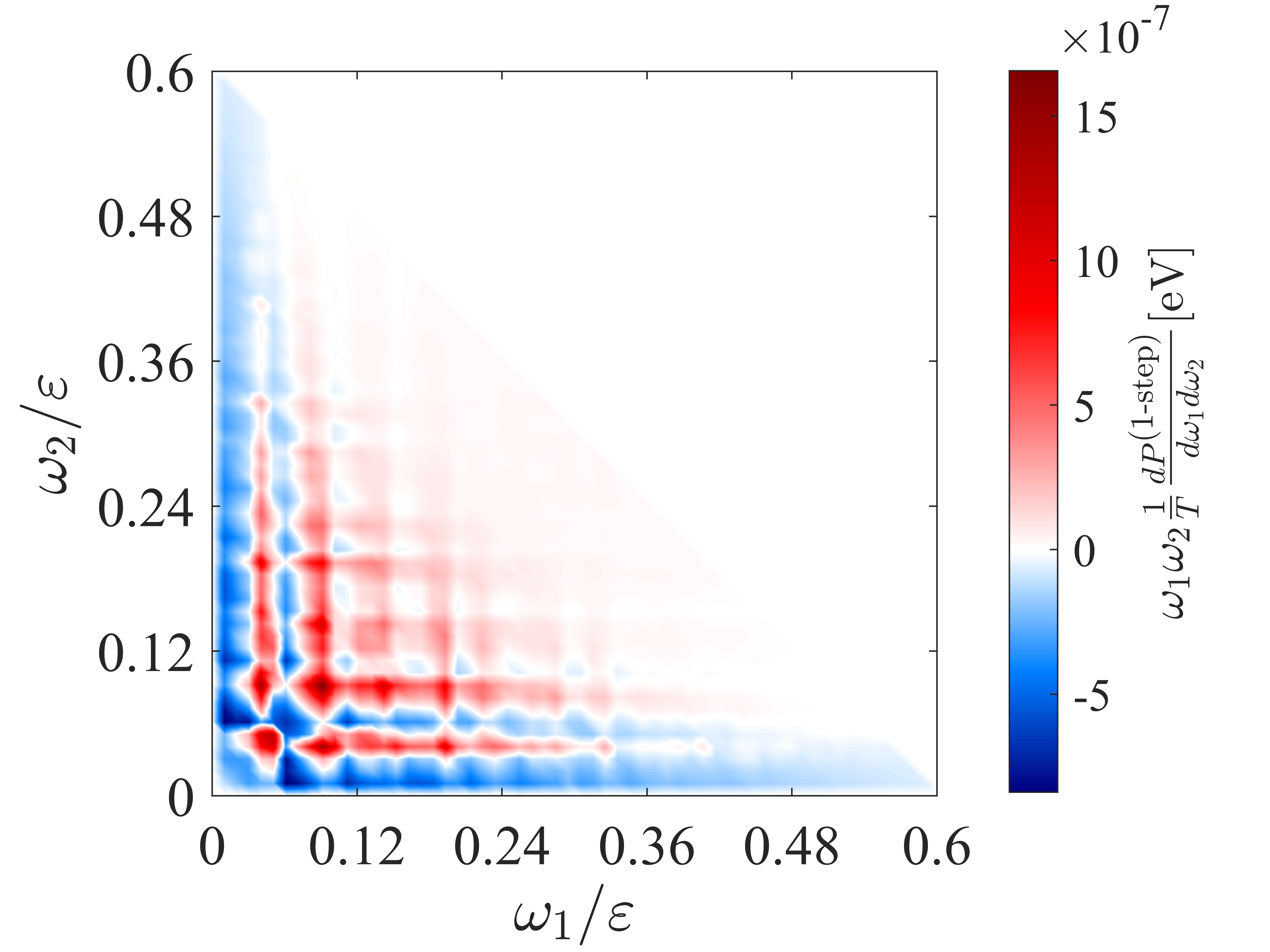
Figure 3: The differential emission probability of two photons with energy
and divided by for the one-step contribution, for
the case mentioned in the text and as in figure (2).
V Discussion of results
In the figures in this paper we show the calculations made for a 180
GeV electron in the Doyle-Turner potential Baier et al. (1998); Doyle and Turner (1968); Avakian et al. (1982); Møller (1995)
for the (110) planes in Silicon and for the state . This is
a quite low lying state which for electrons will have a high radiation
power Wistisen and Di Piazza (2019). Electrons were chosen for this reason
as it is not as numerically heavy when the quantum numbers are relatively
small, as opposed to the positron case, which would require large
quantum numbers to obtain an appreciable value of the quantum non-linearity
parameter , which means that quantum effects such as spin and
recoil are important in the emission process. To compare with an experiment
one should average over the distribution of the initial states which
depends on the particle beam angular mean and divergence. In (41)
the integrals over and are carried out numerically
over the intervals and ,
and therefore includes nearly all emitted radiation. From the result
of Eq. (41) we see that the part scaling with
is the cascade, obtained by simple multiplication of probabilities,
and will dominate unless the crystal is very thin, due to the remaining
terms being proportional to . Therefore, if one made a Monte Carlo
approach using the single photon emission rate using the quantum numbers
of the current state, instead of using the constant field approximation
with the current value of the field, one would obtain the dominant
(cascade) contribution, which will be accurate also when the constant
field approximation is no longer valid. In figure (2)
we show the result from the cascade process. In figure (3)
we show the one-step terms and finally in figure (4)
we show the ratio of these one-step terms to the cascade terms for
. From this figure we see that the one-step
terms can become significant compared to the cascade terms for short
crystals. This ratio scales as . Therefore one needs a thin
crystal for the one-step contribution to be significant, so thin that
the probability to emit more than 1 photon becomes small. One may
rightfully ask based on these figures, if one picks a very small value
of , the total probability could seemingly become negative, however
the results shown are only valid when µm
as estimated earlier. For the GeV case calculated here, the
probability to emit a photon with energy above GeV from a 20
µm crystal is roughly and therefore the probability
corresponding to the cascade for two-photon emission above this photon
energy is , and as can be seen in figure (4)
the spectrum in the region where the radiation is most abundant, the
ratio is around . This number serves as an upper limit to
the size of the effect, because under experimental conditions one
would obtain the average from a population of many different levels
with different quantum number , and this averaging would likely
reduce the size of the effect. If we assume the size of the effect
to be this upper limit, one would need enough events such that one
would have enough statistics to see an effect of such a size from
only of the events. If this setup was realized by adding
a calorimeter to a setup as the one used in Wistisen et al. (2018)
we can estimate the number of particles required to see this.
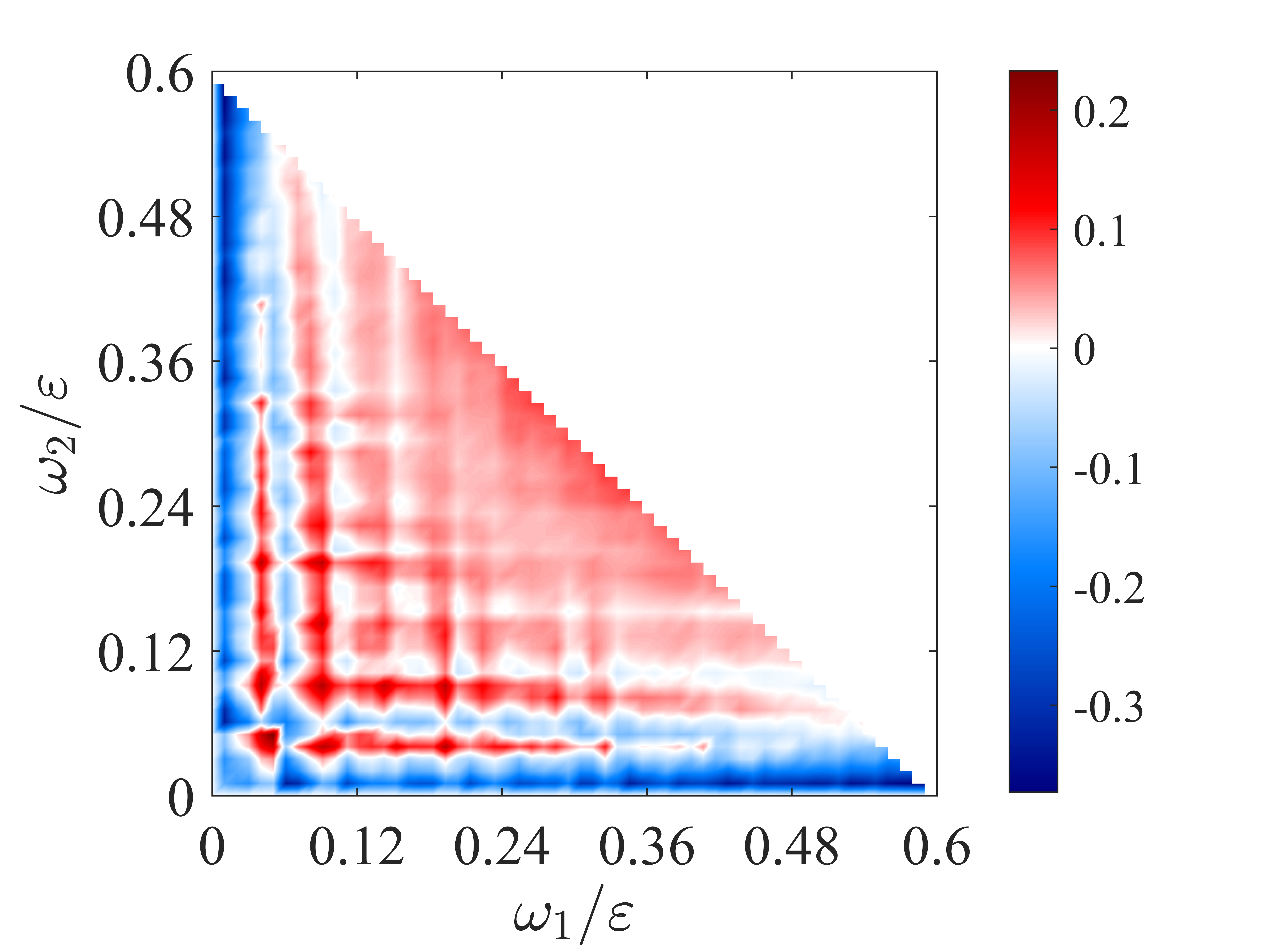
Figure 4: The ratio of emission probabilities of two photons with energy
and for the one-step contribution to the cascade contribution
when m, for the case mentioned in the text and as in figure
(2). This ratio therefore scales as .
Making a histogram of 20 bins in each direction of and
and assuming 100 counts on average in each bin, one
would need roughly electrons and assuming an electron
rate of this translates into roughly 22 days
of measuring time. This would therefore be a challenging experiment
and having in mind that there would likely also be systematic uncertainties,
the realistic outcome of such an experiment would be to put a constraint
on the size of such one-step terms, rather than their direct observation.
VI Conclusion
In conclusion, we have shown how to accurately calculate the two photon
emission rate for a high energy electron (or positron) channeled in
a crystal. This calculation shows that the full probability contains
what is known as the cascade, which could have been obtained multiplying
probabilities of single photon emissions, as well as additional interference
terms, called the one-step contribution. The one-step contribution
scales only linearly with the crystal length, and therefore one needs
a thin crystal to see the effect of these terms. We have calculated
the size of all contributions to the emission probability for 180
GeV electrons in Silicon and found that with a long measuring time,
the one-step contribution could possibly be seen. Since these effects
are however small, we also see how to solve the problem of quantum
radiation reaction, under general circumstances, in a crystal, by
using the single photon emission rate in consecutive emissions, corresponding
to the particle’s current state.
VII Acknowledgments
The author gratefully acknowledges useful discussions with Antonino
Di Piazza and Karen Z. Hatsagortsyan. This work was partially supported
by a research grant (VKR023371) from VILLUM FONDEN and later by the
Alexander von Humboldt-Stiftung. In addition the author acknowledges
the support of NVIDIA Corporation with the donation of the Titan V
GPU used for this research.
Appendix A
The general (unnormalized) solution to the Dirac equation with potential
energy can be written
as
(46)
The Dirac equation then becomes
(47)
(48)
The electron solution is then
(49)
We then obtained an equation for by isolating
in Eq. (48) and inserting in
Eq. (47). This solution has the property that it is
well defined when . Another solution can be found
by isolating in Eq. (47) and
inserting in (48). However this solution is not well
defined when and therefore one must use the negative
energy solution
therefore we have
(50)
where is the positive energy of the positron. The
equation for we can now be obtained by using
(51)
which is equivalent with
(52)
This is the same equation as the one we obtained for ,
except with the sign of changed such that, after making the same
approximations as we did in Wistisen and Di Piazza (2018):
(53)
We therefore make the ansatz in line with the usual approach (the
sign on the momenta is changed):
(54)
(55)
Then
(56)
with ,
inserting , this becomes
(57)
with .
Appendix B
The electron state can be written as (putting back in the volume factor)
(58)
where
(59)
where
and then
(60)
Explicitly we have that . Now since
both and obey that we have
that and therefore can
never be an integer value of unless , and
therefore we can write
(61)
(62)
However the vector is a normalized (),
eigenvector of a hermitian matrix and the vectors corresponding to
and have different eigenvalues of this matrix, and are
therefore orthogonal, so
(63)
Now consider
(64)
and therefore
(65)
There refers only to the normalization. The states are exactly
orthogonal, but in the normalization we neglect corrections which
are suppressed by at least compared to leading order.
So finally
(66)
Appendix C
Even though we consider the radiation from electrons, the propagator
contains terms from the positron .
Therefore we will need to calculate
(67)
and so we need
(73)
(77)
(78)
Then
(79)
(80)
Here we may use that
and so
(81)
Now consider the other part for
(87)
(91)
(92)
This is the same as before except with and
. And now we want the quantity
(93)
where now is chosen such that
is in the FBZ. Note that
for which we already have the solution, called ,
and therefore
(94)
therefore . For the
term one obtains that and
for this term one has that , in terms
of the value for the corresponding electron term in
the propagator. And that the index is given by .
Appendix D
We need to consider ,
in particular we would like to show that
is 0, where the arrows denote the spin state of the virtual particle.
This we may rearrange and consider therefore the product .
Now we may use that can be written as
(95)
Now for simplicity we define
(96)
(97)
and then we have that
(98)
Therefore
(99)
We assume that ,
which is possible if we choose linear polarization as our basis, and
we will perform the summation of final spins and therefore
is the identity
(100)
where we used that is a real vector. For
the other term,
the same can be done, and here the argument hinges upon summation
over initial spins, therefore, if either a summation is carried out
over initial or final spins, the spin interference terms will be 0.
References
Lindhard (1965)J. Lindhard, “Influence of
crystal lattice on motion of energetic charged particles,” K. Dan. Vidensk. Selsk. Mat.
Fys. Medd. 34, no. 14,
1–64 (1965).
Bak et al. (1985)J. Bak, J.A. Ellison,
B. Marsh, F.E. Meyer, O. Pedersen, J.B.B. Petersen, E. Uggerhøj, K. Østergaard, S.P. Møller, A.H. Sørensen, and M. Suffert, “Channeling radiation from 2-55 GeV/c electrons and
positrons: (I). Planar case,” Nucl. Phys. B. 254, 491 – 527 (1985).
Bak et al. (1988)J.F. Bak, J.A. Ellison,
B. Marsh, F.E. Meyer, O. Pedersen, J.B.B. Petersen, E. Uggerhøj, S.P. Møller, H. Sørensen, and M. Suffert, “Channeling radiation from 2 to 20 GeV/c electrons and
positrons (II).: Axial case,” Nucl. Phys. B. 302, 525 – 558 (1988).
Swent et al. (1979)R. L. Swent, R. H. Pantell,
M. J. Alguard, B. L. Berman, S. D. Bloom, and S. Datz, “Observation of channeling radiation from relativistic
electrons,” Phys. Rev. Lett. 43, 1723–1726 (1979).
Andersen et al. (1981)J.U. Andersen, K.R. Eriksen, and E. Laegsgaard, “Planar-Channeling Radiation and Coherent Bremsstrahlung for MeV
Electrons,” Phys. Scr. 24, 588 (1981).
Klein et al. (1985)R. K. Klein, J. O. Kephart,
R. H. Pantell, H. Park, B. L. Berman, R. L. Swent, S. Datz, and R. W. Fearick, “Electron channeling radiation from diamond,” Phys. Rev. B 31, 68–92 (1985).
Alguard et al. (1979)M. J. Alguard, R. L. Swent,
R. H. Pantell, B. L. Berman, S. D. Bloom, and S. Datz, “Observation of radiation from channeled positrons,” Phys. Rev. Lett. 42, 1148–1151 (1979).
Andersen et al. (2012)K. K. Andersen, J. Esberg,
H. Knudsen, H. D. Thomsen, U. I. Uggerhøj, P. Sona, A. Mangiarotti, T. J. Ketel, A. Dizdar, and S. Ballestrero (CERN NA63), “Experimental investigations of synchrotron
radiation at the onset of the quantum regime,” Phys.
Rev. D 86, 072001
(2012).
Uggerhøj (2005)U. I. Uggerhøj, “The
interaction of relativistic particles with strong crystalline fields,” Rev. Mod. Phys. 77, 1131–1171 (2005).
Kumakhov (1976)M.A. Kumakhov, “On the theory
of electromagnetic radiation of charged particles in a crystal,” Phys. Lett. A 57, 17 – 18 (1976).
Kumakhov (1977)M.A. Kumakhov, “Theory of
radiation of charged particles channeled in a crystal,” Phys. Status Solidi B 84, 41–54 (1977).
Sáenz et al. (1981)A.W. Sáenz, H. Überall, and A. Nagl, “Calculation of
electron channeling radiation with a realistic potential,” Nucl. Phys. A. 372, 90 – 108 (1981).
Kimball and Cue (1985)J.C. Kimball and N. Cue, “Quantum electrodynamics and
channeling in crystals,” Phys. Rep. 125, 69 – 101 (1985).
Belkacem et al. (1986)A. Belkacem, G. Bologna,
M. Chevallier, N. Cue, M.J. Gaillard, R. Genre, J.C. Kimball, R. Kirsch, B. Marsh, J.P. Peigneux, J.C. Poizat, J. Remillieux, D. Sillou,
M. Spighel, and C.R. Sun, “New channeling effects in the radiative
emission of 150 gev electrons in a thin germanium crystal,” Phys. Lett. B 177, 211 – 216 (1986).
Esberg et al. (2010)J. Esberg, K. Kirsebom,
H. Knudsen, H. D. Thomsen, E. Uggerhøj, U. I. Uggerhøj, P. Sona, A. Mangiarotti, T. J. Ketel, A. Dizdar, M. M. Dalton,
S. Ballestrero, and S. H. Connell (CERN NA63), “Experimental investigation of strong field trident production,” Phys. Rev. D 82, 072002 (2010).
Wistisen et al. (2018)T. N. Wistisen, A. Di Piazza,
H. V. Knudsen, and U. I. Uggerhøj, “Experimental evidence of
quantum radiation reaction in aligned crystals,” Nat. Commun. 9, 795 (2018).
Bula et al. (1996)C. Bula, K.T. McDonald,
E.J. Prebys, C. Bamber, S. Boege, T. Kotseroglou, A.C. Melissinos, D.D. Meyerhofer, W. Ragg, D.L. Burke, et al., “Observation of nonlinear effects in compton scattering,” Phys. Rev. Lett. 76, 3116 (1996).
Seipt and Kämpfer (2012)Daniel Seipt and Burkhard Kämpfer, “Two-photon
compton process in pulsed intense laser fields,” Phys.
Rev. D 85, 101701
(2012).
Mackenroth and Di Piazza (2013)F. Mackenroth and A. Di Piazza, “Nonlinear
Double Compton Scattering in the Ultrarelativistic Quantum Regime,” Phys. Rev. Lett. 110, 070402 (2013).
Dinu and Torgrimsson (2018a)V. Dinu and G. Torgrimsson, “Single,
double and higher-order nonlinear Compton scattering,” arXiv preprint arXiv:1811.00451 (2018a).
Baier and Katkov (1968)V.N. Baier and V.M. Katkov, “Processes
involved in the motion of high energy particles in a magnetic field,” J. Exp. Theor.
Phys. 26, 854 (1968).
Baier et al. (1998)V.N. Baier, V.M. Katkov, and V.M. Strakhovenko, Electromagnetic Processes at High
Energies in Oriented Single Crystals (World
Scientific, 1998).
Wistisen (2015)T. N. Wistisen, “Quantum
synchrotron radiation in the case of a field with finite extension,” Phys. Rev. D 92, 045045 (2015).
Wistisen and Di Piazza (2019)Tobias N. Wistisen and Antonino Di Piazza, “Complete treatment of single-photon emission in planar channeling,” (2019), arXiv:1904.02997 [hep-ph] .
Wistisen and Di Piazza (2018)T. N. Wistisen and A. Di Piazza, “Impact of
the quantized transverse motion on radiation emission in a Dirac harmonic
oscillator,” Phys. Rev. A 98, 022131 (2018).
Hu et al. (2010)Huayu Hu, Carsten Müller,
and Christoph H. Keitel, “Complete QED
Theory of Multiphoton Trident Pair Production in Strong Laser Fields,” Phys. Rev. Lett. 105, 080401 (2010).
Acosta and Kämpfer (2019)Uwe Hernandez Acosta and Burkhard Kämpfer, “Laser pulse-length effects in trident pair production,” arXiv preprint arXiv:1901.08860 (2019).
King and Fedotov (2018)B. King and A. M. Fedotov, “Effect of
interference on the trident process in a constant crossed field,” Phys. Rev. D 98, 016005 (2018).
Dinu and Torgrimsson (2018b)V. Dinu and G. Torgrimsson, “Trident
pair production in plane waves: Coherence, exchange, and spacetime
inhomogeneity,” Phys. Rev. D 97, 036021 (2018b).
Mackenroth and Di Piazza (2018)F. Mackenroth and A. Di Piazza, “Nonlinear
trident pair production in an arbitrary plane wave: A focus on the properties
of the transition amplitude,” Phys. Rev. D 98, 116002 (2018).
Doyle and Turner (1968)P. A. Doyle and P. S. Turner, “Relativistic
Hartree–Fock X-ray and electron scattering factors,” Acta
Crystallogr. A 24, 390–397 (1968).
Avakian et al. (1982)A.L. Avakian, N.K. Zhevago,
and Shi Yan, “Emission of electrons and
positrons in the axial semichanneling,” J. Exp. Theor. Phys. 82, 573–586 (1982).
Di Piazza et al. (2010)A. Di Piazza, K. Z. Hatsagortsyan, and C. H. Keitel, “Quantum Radiation Reaction Effects in Multiphoton Compton Scattering,” Phys. Rev. Lett. 105, 220403 (2010).
Poder et al. (2018)K. Poder, M. Tamburini,
G. Sarri, A. Di Piazza, S. Kuschel, C. D. Baird, K. Behm, S. Bohlen, J. M. Cole,
D. J. Corvan, M. Duff, E. Gerstmayr, C. H. Keitel, K. Krushelnick, S. P. D. Mangles, P. McKenna, C. D. Murphy, Z. Najmudin, C. P. Ridgers, G. M. Samarin, D. R. Symes, A. G. R. Thomas, J. Warwick, and M. Zepf, “Experimental
signatures of the quantum nature of radiation reaction in the field of an
ultraintense laser,” Phys. Rev. X 8, 031004 (2018).
Cole et al. (2018)J. M. Cole, K. T. Behm,
E. Gerstmayr, T. G. Blackburn, J. C. Wood, C. D. Baird, M. J. Duff, C. Harvey, A. Ilderton, A. S. Joglekar, K. Krushelnick, S. Kuschel, M. Marklund,
P. McKenna, C. D. Murphy, K. Poder, C. P. Ridgers, G. M. Samarin, G. Sarri, D. R. Symes,
A. G. R. Thomas, J. Warwick, M. Zepf, Z. Najmudin, and S. P. D. Mangles, “Experimental evidence of radiation reaction in the collision of a
high-intensity laser pulse with a laser-wakefield accelerated electron
beam,” Phys. Rev. X 8, 011020 (2018).
Neitz and Di Piazza (2013)N. Neitz and A. Di Piazza, “Stochasticity
effects in quantum radiation reaction,” Phys. Rev. Lett. 111, 054802 (2013).
Blackburn et al. (2014)T. G. Blackburn, C. P. Ridgers, J. G. Kirk, and A. R. Bell, “Quantum radiation reaction
in laser–electron-beam collisions,” Phys. Rev. Lett. 112, 015001 (2014).
Vranic et al. (2016)Marija Vranic, Thomas Grismayer, Ricardo A Fonseca, and Luis O Silva, “Quantum radiation
reaction in head-on laser-electron beam interaction,” New Journal of Physics 18, 073035 (2016).
Li et al. (2014)Jian-Xing Li, Karen Z. Hatsagortsyan, and Christoph H. Keitel, “Robust signatures of quantum radiation reaction in focused ultrashort laser
pulses,” Phys. Rev. Lett. 113, 044801 (2014).
Beresteckij et al. (2008)Vladimir B Beresteckij, Evgenij M Lifsic, and Lev P Pitaevskij, Quantum electrodynamics (Butterworth-Heinemann, Oxford, 2008).
Feynman (1965)Richard P Feynman, Feynman
lectures on physics. Volume 3: Quantum mechancis (1965).
Hu (2011)Huayu Hu, Multi-photon creation and
single-photon annihilation of electron-positron pairs (2011).
Oleinik (1967)V.P. Oleinik, “Resonance
effects in the field of an intense laser beam,” J. Exp. Theor. Phys. 25, 697 (1967).
Oleinik (1968)V.P. Oleinik, “Resonance
effects in the field of an intense laser ray. ii,” J. Exp. Theor. Phys. 26, 1132 (1968).
Roshchupkin (1996)S.P. Roshchupkin, “Resonant
effects in collisions of relativistic electrons in the field of a light
wave,” Laser
Phys. 6, 837–858
(1996).
Lötstedt et al. (2007)Erik Lötstedt, Ulrich D. Jentschura, and Christoph H. Keitel, “Evaluation of laser-assisted bremsstrahlung with dirac-volkov
propagators,” Phys. Rev. Lett. 98, 043002 (2007).
Gonthier et al. (2014)Peter L. Gonthier, Matthew G. Baring, Matthew T. Eiles, Zorawar Wadiasingh, Caitlin A. Taylor, and Catherine J. Fitch, “Compton scattering in strong magnetic fields:
Spin-dependent influences at the cyclotron resonance,” Phys.
Rev. D 90, 043014
(2014).
Bransden et al. (2003)Brian Harold Bransden, Charles Jean Joachain, and Theodor J Plivier, Physics of atoms and molecules (Pearson
Education India, 2003).