Applications of Grassmannian flows to integrable systems

Abstract

We show how many classes of partial differential systems with local and nonlocal nonlinearities are linearisable in the sense that they are realisable as Fredholm Grassmannian flows. In other words, time-evolutionary solutions to such systems can be constructed from solutions to the corresponding underyling linear partial differential system, by solving a linear Fredholm equation. For example, it is well-known that solutions to classical integrable partial differential systems can be generated by solving a corresponding linear partial differential system for the scattering data and then solving the linear Fredholm (or Volterra) integral equation known as the Gel’fand–Levitan–Marchenko equation. In this paper and in a companion paper, Doikou et al. DMSW:graphflows , we both, survey the classes of nonlinear systems that are realisable as Fredholm Grasssmannian flows, and present new example applications of such flows. We also demonstrate the usefulness of such a representation. Herein we extend the work of Pöppe and demonstrate how solution flows of the noncommutative potential Korteweg de Vries and nonlinear Schrödinger systems are examples of such Grassmannian flows. In the companion paper we use this Grassmannian flow approach as well as an extension to nonlinear graph flows, to solve Smoluchowski coagulation and related equations.

1 Introduction

Our goal herein is to demonstrate that many classes of partial differential systems with local and nonlocal nonlinearities are realisable as Fredholm Grassmannian flows. In essence this means their solution flow can be generated as the solution to a corresponding set of linear partial differential systems together with a linear Fredholm integral equation. In the context of classical integrable systems, the linear Fredholm integral equation is the Gel’fand–Levitin–Marchenko equation. In the more general unifying context of Grassmannian flows, the linear Fredholm equation represents the linear relation whose solution is the linear projection map from the Fredholm Stiefel manifold to the Fredholm Grassmann manifold in a given Hilbert–Schmidt coordinate chart. We call it the linear Fredholm kernel equation. Note, the Fredholm Grassmann manifold can be thought of as consisting of all collections of graphs of compatible linear Hilbert–Schmidt maps. In Beck, Doikou, Malham and Stylianidis BDMS1 ; BDMS2 , we demonstrated the solution flows of many classes of partial differential systems with nonlocal nonlinearities are Grassmannian flows. Here, we extend the class of flows which are Grassmannian flows to include some classical integrable systems. In a companion paper, Doikou et al. DMSW:graphflows , we extend the class of Grassmannian flows to include the Smoluchowski coagulation and related equations in the case of a constant frequency kernel. We also we introduce the notion of graph flows, nonlinear generalisations of Grassmannian flows, which incorporate the Smoluchowski coagulation equation for the cases of additive and multiplicative frequency kernels.

The unifying approach to solving nonlinear partial differential equations we develop herein has its roots in computational spectral theory where Grassmannian flows were developed to deal with numerical difficulties associated with different exponential growth rates in the far-field for large (high order) systems, see Ledoux, Malham and Thümmler LMT and Ledoux, Malham, Niesen and Thümmler LMNT as well as Karambal and Malham KM . In Beck and Malham BM Grassmannian flows and representative coordinate patches were instrumental to the characterisation and computation of the Maslov index for large systems. This led to the need to develop the theory of Fredholm Grassmannian flows and thus nonlinear partial differential systems. We were then motivated by a sequence of papers by Pöppe P-SG ; P-KdV ; P-KP , Pöppe and Sattinger PS-KP and Bauhardt and Pöppe BP-ZS . Pöppe’s work was recently revisited by McKean McKean . These papers advocated, at the operator level, the solution of classical integrable systems by solving a linearised version of the system at hand together with a Marchenko operator relation. This was the natural development from classical constructions of this type suggested and developed in particular by Miura Miura , Dyson Dyson and Ablowitz, Ramani and Segur ARSII . Also see Nijhoff, Quispel, Van Der Linden and Capel NQVDLCI , Nijhoff, Quispel, Capel NQVDLCII , Mumford Mumford , Fordy and Kulisch FK and Tracy and Widom TW . Of specific interest to us in Pöppe’s papers was that the structure underlying the approach advocated therein appeared to be that of a Fredholm Grassmannian. We exploited this perspective in Beck et al. BDMS1 ; BDMS2 where we first explored this question and showed how to solve classes of partial differential systems with nonlocal nonlinearities—we explain what we mean by such systems presently.

Explicitly, though formally for the moment, the essential ideas underlying the Pöppe programme we advocate here can be summarised as follows. First let us define the unifying canonical system of operator equations underlying all the systems we consider herein as well as in Doikou et al. DMSW:graphflows .

Definition 1 (Canonical system)

Suppose the time-dependent Hilbert–Schmidt operators $Q=Q(t)$, $P=P(t)$ and $G=G(t)$ satisfy the following system of operator equations, with $Q\coloneqq{\mathrm{id}}-\hat{Q}$:

$${\partial}_{t}Q =A(t,Q,P)\,Q+B(t,Q,P)\,P,$$

$${\partial}_{t}P =C(t,Q,P)\,Q+D(t,Q,P)\,P,$$

$$P =GQ.$$

Here $A$, $B$, $C$ and $D$ are known operators which, in general, depend on $t$, $Q$ and $P$.

Suppose $Q(0)=Q_{0}$ and $P(0)=P_{0}$ for some given data $Q_{0}$ and $P_{0}$ such that $\hat{Q}_{0}$ and $P_{0}$ are Hilbert–Schmidt operators. Further assume there exists a solution to the pair of evolutionary equations for $Q=Q(t)$ and $P=P(t)$ shown in the canonical system in Definition 1, in the sense that $\hat{Q}=\hat{Q}(t)$ and $P=P(t)$ are Hilbert–Schmidt operators for $t\in[0,T]$ for some $T>0$. If the Fredholm operator $Q=Q(t)$ and Hilbert–Schmidt operator $P=P(t)$ are related by the operator $G=G(t)$ shown in the third equation at least for some time $t\in[0,T]$ for some $T>0$, then a straightforward calculation shows that if $Q=Q(t)$ and $P=P(t)$ satisfy the canonical system above, then $Q=Q(t)$ and $G=G(t)$ satisfy the coupled system of equations:

$${\partial}_{t}Q= \;A(t,Q,GQ)\,Q+B(t,Q,GQ)\,(GQ),$$

$${\partial}_{t}G= \;\bigl{(}C(t,Q,GQ)\,Q\bigr{)}\,Q^{-1}+\bigl{(}D(t,Q,GQ)\,(GQ)\bigr{)}\,Q^{-1}$$

$$\;-G\bigl{(}A(t,Q,GQ)\,Q+B(t,Q,GQ)\,(GQ)\bigr{)}\,Q^{-1},$$

for $t\in[0,T^{\prime}]$ for some $0<T^{\prime}\leqslant T$.

Typically we choose the operators $A$, $B$, $C$ and $D$ so that the canonical system of equations in Definition 1 is linear. And further, typically, for the choices of $A$, $B$, $C$ and $D$ we make, the evolution equation for the operator for $G$ decouples from that for $Q$—though the evolution equation for $Q$ may still depend on $G$. All the systems considered in Beck et al. BDMS1 ; BDMS2 , as well as some of the Smoluchowski-type coagulation systems in our companion paper Doikou et al. DMSW:graphflows , fall into this category. We briefly survey these cases now. Note that we have assumed that for $t\in[0,T]$ for some $T>0$, there exist solutions $Q$ and $P$ to the canonical system in Definition 1 such that $\hat{Q}$ and $P$ are Hilbert–Schmidt operators. As we shall see, as a consequence $G$ is also Hilbert–Schmidt valued. This means that $\hat{Q}$, $P$ and $G$ have representations in terms of square-integrable kernel functions, say, respectively $\hat{q}=\hat{q}(x,y;t)$, $p=p(x,y;t)$ and $g=g(x,y;t)$. Hence the linear relation $P=GQ$ between $Q$ and $P$, which hereafter we shall denote the linear Fredholm equation, has the form

$$p(x,y;t)=g(x,y;t)-\int g(x,z;t)\hat{q}(z,y;t)\,{\mathrm{d}}z.$$

The interval of integration, and any further properties assumed for the kernel functions $\hat{q}$, $p$ and $g$, depend on the context/application at hand. For example, suppose the operators $A=C=O$ while $B=-{\partial}_{x}$ and $D=d({\partial}_{x})$ where $d$ is a constant coefficient polynomial function of its argument. Then the canonical system reduces to the linear pair of partial differential equations ${\partial}_{t}p=d({\partial}_{x})p$ and ${\partial}_{t}\hat{q}=-{\partial}_{x}p$. The evolution equation for $G=G(t)$, in terms of its kernel $g=g(x,y;t)$ becomes (note the interval of integration is ${\mathbb{R}}$):

$${\partial}_{t}g(x,y;t)=d({\partial}_{x})g(x,y;t)+\int_{\mathbb{R}}g(x,z;t){\partial}_{z}g(z,y;t)\,{\mathrm{d}}z.$$

This nonlocal nonlinear partial differential equation is typical of the many examples presented in Beck et al. BDMS1 ; BDMS2 . Such classes of nonlinear partial differential equations have two underlying characteristics. The first is that the nonlinearity is nonlocal as shown and we think of it as the generalisation from a product of matrix operators to the infinite dimensional analogue of the kernel representation of the product of a pair of infinite-dimensional Hilbert–Schmidt operators, here between $G$ and ${\partial}_{x}G$. We call the integral term above the ‘big matrix product’ and at the kernel level express it as $g\star({\partial}g)$, i.e. for any two kernels $g=g(x,y)$ and $g^{\prime}=g^{\prime}(x,y)$ we write

$$\bigl{(}g\star g^{\prime}\bigr{)}(x,y)\coloneqq\int_{\mathbb{R}}g(x,z)g^{\prime}(z,y)\,{\mathrm{d}}z.$$

The second characteristic is that the unbounded operators shown $d=d({\partial}x)$ for $D$ and $-{\partial}_{x}$ for $B$, only act on the first arguments of the kernel functions. Now assume, instead of the form above, the operator $B$ corresponds to minus the identity operator so that ${\partial}_{t}q=-p$. Then a special subclass we can consider here is to suppose the linear relation $P=GQ$ has a convolutional form so that,

$$p(x,y;t)=g(x-y;t)-\int_{\mathbb{R}}g(x-z;t)\hat{q}(z,y;t)\,{\mathrm{d}}z.$$

Then the evolution equation for $G=G(t)$, after setting $y=0$ becomes (again for the moment the interval of integration is ${\mathbb{R}}$):

$${\partial}_{t}g(x;t)=d({\partial}_{x})g(x;t)+\int_{\mathbb{R}}g(x-z;t)g(z;t)\,{\mathrm{d}}z.$$

See Beck et al. (BDMS1, , Sec. 1.4) for more details. If we restrict the interval of integration to $[0,\infty)$ then this form of equation demonstrates how we can treat Smoluchowski-type coagulation equations with constant frequency kernels in this manner. Indeed this is the basis for the multitude of examples we consider in our companion paper Doikou et al. DMSW:graphflows . Within this class of ‘big matrix product’ equations, another example is insightful. Hitherto, the nonlinearity in the resulting equation for $g=g(x,y;t)$ was generated by the term associated with the operator $B$. This term corresponds to the quadratic term that appears in the Riccati equation ${\partial}_{t}G=C+DG-G(A+BG)$, that results from assuming $A$, $B$, $C$ and $D$ are functions of $t$ only, or if we allow $B$ and $D$ to also have the dependence on ${\partial}_{x}$ indicated above. However, now suppose in the canonical system, the operators $B=C=O$ while $A(t,Q,P)=-\mathrm{i}f(PP^{\dagger})$ and $D=-\mathrm{i}h({\partial}_{x})$ where $h$ and $f$ are real constant coefficient polynomials of their arguments with $h$ even, and $P^{\dagger}$ represents the operator adjoint to $P$. Hence the canonical system reduces to the linear pair of partial differential equations ${\partial}_{t}p=-\mathrm{i}h({\partial}_{x})p$ and ${\partial}_{t}\hat{q}=-\mathrm{i}f^{\star}(p\star p^{\dagger})\star q$, where now $p^{\dagger}$ represents the kernel of $P^{\dagger}$ and $q=\delta-\hat{q}$, with the ‘$\delta$’ representing the identity operator at the kernel level, in particular $\delta\star q^{\prime}=q^{\prime}\star\delta=q^{\prime}$ for any Hilbert–Schmidt kernel $q^{\prime}$. Note the ‘$\star$’ is the big matrix product above, and $f^{\star}$ represents the same polynomial as $f$, but the product given by ‘$\star$’. In this case the evolution equation for $G=G(t)$, i.e. for the kernel $g=g(x,y;t)$, becomes (see Beck et al. BDMS2 for the details):

$$\mathrm{i}{\partial}_{t}g=h({\partial}_{x})g+g\star f^{\star}(g\star g^{\dagger}).$$

If $f(x)=x$, then this equation represents the nonlocal nonlinear Schrödinger equation, with the product the nonlocal big matrix product. Note the nonlinearity is generated by the term corresponding to the operator $A$. Further note, the canonical system here is linear in the sense that we can solve the linear equation for $p=p(x,y;t)$ first, and then substitute its solution form into the evolution equation ${\partial}_{t}\hat{q}=-\mathrm{i}f^{\star}(p\star p^{\dagger})\star q$ for $q=q(x,y;t)$ which is linear. See Beck et al. BDMS2 for more details.

Let us now examine the connection between the canonical system in Definition 1 and classical integrable systems. Some further layers of structure are also required. As discussed above, and in particular motivated by the results in Ablowitz, Ramani and Segur ARSII and in the sequence of papers by Pöppe, we know that solutions to classical nonlinear integrable systems can be generated from solutions to the corresponding linearised versions of these equations by solving the corresponding Gel’fand–Levitan–Marchenko equation. At the operator level, say for the Korteweg–de Vries case, we suppose ${\partial}_{t}P=\mu{\partial}_{x}^{n}P$ and $\hat{Q}=P$, so that $P=G({\mathrm{id}}-P)$. Here $\mu\in{\mathbb{R}}$ is a constant and $n\geqslant 3$. With reference to the canonical system in Definition 1, this corresponds to setting $B=C=O$ and $A=D=\mu{\partial}_{x}^{n}$ so that the canonical system and linear Fredholm relation reduce to,

$${\partial}_{t}Q =\mu{\partial}_{x}^{n}Q,$$

$${\partial}_{t}P =\mu{\partial}_{x}^{n}P,$$

$$P =GQ.$$

In the Korteweg–de Vries equation context, the scattering data corresponding to the Hilbert–Schmidt operator $P$ with kernel $p$ is assumed to be additive. By this we mean the following. If $y$ and $z$ are the variables parameterising the Hilbert–Schmidt kernel $p=p(y,z;t)$ corresponding to $P$, then we assume $p$ has the form $p=p(y+z;t)$. Operators with such additive kernels are known as Hankel operators. Further we assume the operator $P$ depends on a parameter $x\in{\mathbb{R}}$ in an additive way so that it has the form $p=p(y+z+x;t)$. For this form, we can equivalently use ${\partial}_{y}$, ${\partial}_{z}$ or ${\partial}_{x}$ in the system of equations for the operators above, indeed, naturally we only need to solve the corresponding kernel equations in terms of a single variable, eg. we only need to solve ${\partial}_{t}p=\mu{\partial}_{y}^{n}p$ for $p=p(y;t)$. With $p$ and thus $P$ in hand, $\hat{Q}$ is automatically given as $\hat{Q}=P$. Further in this context the linear Fredholm kernel equation has the form (note the interval of integration is now $(-\infty,0]$),

$$p(y+z+x;t)=g(y,z;x,t)-\int_{-\infty}^{0}g(y,\xi;x,t)p(\xi+z+x;t)\,{\mathrm{d}}\xi.$$

If we set $y=0$ and making a change of variables, this relation can be shown to be precisely the Gel’fand–Levitan–Marchenko equation; see Remark 27 for the details. Hence thusfar, we have precisely the setup for the inverse scattering transform. Classically the procedure is now, using that the function $p$ satisfies the linear Korteweg–de Vries equation and has an additive form, to differentiate the Fredholm equation above and show that $g=g(0,0;x,t)$ satisfies the potential Korteweg–de Vries equation. Note, setting $z=0$ in $g=g(0,z;x,t)$ is equivalent to evaluating the unknown in the Gel’fand–Levitan–Marchenko equation along the diagonal. However herein, motivated by the work of Pöppe, we prefer to keep the subsequent computation at the operator level. Recall our choices for the operators $A$, $B$, $C$ and $D$ in this case. The evolution equation for $G=G(t)$ here has the form:

$${\partial}_{t}G=\mu{\partial}_{x}^{n}(GQ)\,Q^{-1}-\mu G({\partial}_{x}^{n}Q)\,Q^{-1}.$$

Setting $U\coloneqq({\mathrm{id}}-P)^{-1}$, using that $U={\mathrm{id}}+PU={\mathrm{id}}+UP$ so ${\partial}_{t}G={\partial}_{t}U$ and also ${\partial}_{t}G=U({\partial}_{t}P)U$, a more succinct version of this last relation is,

$${\partial}_{t}G=\mu U({\partial}_{x}^{n}P)U.$$

This is still not a closed form equation for $G=G(t)$, however our goal is to derive a closed form nonlinear equation for its kernel $g=g(y,z;x,t)$. We also want to develop a systematic procedure to do this. To achieve both, following Pöppe, we now incorporate some additional implicit structure we have not utilised thusfar. For any given Hilbert–Schmidt operator say $G$, let $[G]$ denote its square-integrable kernel so $[G]=g$. We denote the operator $[\,\cdot\,]$ the bracket operator. Thusfar we have not used that $P$ is a Hankel operator, for which the following crucial product rule holds. Suppose $F$ and $F^{\prime}$ are Hilbert–Schmidt operators and that $H$ and $H^{\prime}$ are Hilbert–Schmidt Hankel operators, dependent on parameters $x\in{\mathbb{R}}$ and $t\geqslant 0$. Then the fundamental theorem of calculus implies the following product rule (the Pöppe product rule, see Lemma 2):

$$[F{\partial}_{x}(HH^{\prime})F^{\prime}](y,z;x,t)\equiv[FH](y,0;x,t)[H^{\prime}F^{\prime}](0,z;x,t).$$

The goal now is to apply the bracket operator to the evolution equation for $G$ above, and see if the bracket operator applied to the sequence of operators $U({\partial}_{x}^{n}P)U$ generates a closed form in $[G]$. The answer in this instance is positive, and after relatively small effort we can show (see Theorem 5.1) that for the $n=3$ case,

$$\bigl{[}U({\partial}_{x}^{3}P)U\bigr{]}(y,z;x,t)={\partial}_{x}^{3}[G](y,z;x,t)-3\,\bigl{(}{\partial}_{x}[G](y,0;x,t)\bigr{)}\bigl{(}{\partial}_{x}[G](0,z;x,t)\bigr{)}.$$

Thus $g(y,z;x,t)=[G](y,z;x,y)$ satisfies the nonlinear partial differential equation,

$${\partial}_{t}g(y,z;x,t)=\mu{\partial}_{x}^{3}g(y,z;x,t)-3\bigl{(}({\partial}_{x}g)(y,0;x,t)\bigr{)}\bigl{(}({\partial}_{x}g)(0,z;x,t)\bigr{)}.$$

Actually here we have a whole set of nonlocal nonlinear equations for each $y$ and $z$. The nonlocal nonlinearity is the second notion of nonlocal nonlinearity we mention herein. Importantly however, we notice that if we set $y=z=0$ then $g=g(0,0;x,t)$ satisfies the the potential Korteweg–de Vries equation (with usual local nonlinearity),

$${\partial}_{t}g(0,0;x,t)=\mu{\partial}_{x}^{3}g(0,0;x,t)-3\mu\bigl{(}({\partial}_{x}g)(0,0;x,t)\bigr{)}^{2}.$$

Let us summarise the procedure just outlined. We start with a simple linear evolutionary partial differential equation for the scattering data operator $P=P(t)$, which we assume is a Hilbert–Schmidt Hankel operator. This equation represents the linear version of the target nonlinear integrable partial differential equation. We set $\hat{Q}\coloneqq P$. We define an evolutionary Hilbert–Schmidt operator $G=G(t)$ via the Fredholm equation $P=G({\mathrm{id}}-\hat{Q})$. Then by a systematic computation we derive an evolution equation for $G=G(t)$, in which the flow-field, i.e. the right-hand side in the equation ${\partial}_{t}G=\cdots$, depends in general on $P$ and $U\coloneqq({\mathrm{id}}-\hat{Q})^{-1}$. The evolutionary operator $Q={\mathrm{id}}-\hat{Q}$ itself satisfies an evolutionary equation with a flow-field that depends on $Q$ and $G$—see the discussion immediately following Definition 1. However we focus on the equation for $G=G(t)$, and see if we can write the flow-field, at the level of the operator kernels as a closed form in terms of the kernel or ${\partial}_{x}$ derivatives of the kernel—this is where we applied the bracket operator and then utilised the product rule. It turns out, though this is relatively obscure presently, that this latter procedure where we try to express the flow-field for $[G]=[G](t)$ as a closed form in terms of $[G]$ or spatial partial derivatives of $[G]$ is highly systematic and boils down to algebraic polynomial construction. See for example Malham Malham:KdVhierarchy . Our belief is that it is this systematic structure/procedure, initiated by Pöppe, that represents the major advantage of his approach.

Let us briefly consider one more example we tackle herein, the noncommutative nonlinear Schrödinger equation. At the operator level we suppose the Hilbert–Schmidt Hankel operator $P=P(t)$ satisfies the linear dispersive system ${\partial}_{t}P=-\mu_{n}(\mathrm{i}\mathcal{I})^{n-1}{\partial}_{x}^{n}P$, where $\mu_{n}\in{\mathbb{R}}$ is a constant and $\mathcal{I}\coloneqq\mathrm{diag}\{-{\mathrm{id}},{\mathrm{id}}\}$, i.e. the diagonal square matrix with the upper left and lower right blocks as indicated. Further we set $\hat{Q}=P^{2}$. We can in principle fit this into the canonical system in Definition 1, though there is no need as we already have the necessary prescibed linear evolution in terms of $P$ and $\hat{Q}$. As for the Korteweg–de Vries case, it is convenient to set $U\coloneqq({\mathrm{id}}-\hat{Q})^{-1}$. A straightforward calculation shows (see Remark 21) that,

$${\partial}_{t}G=-\mu_{n}(\mathrm{i}\mathcal{I})^{n-1}\bigl{(}U({\partial}_{x}^{n}P)U+(-1)^{n-1}G({\partial}_{x}^{n}P)G\bigr{)}.$$

As we did for the potential Korteweg–de Vries equation above, we apply the bracket operator and see if the bracket operator applied to the right-hand side above generates a closed form in $[G]$. Again, after relatively small effort we can show (see Theorem 6.1) that for the $n=2$ case,

$$\bigl{[}U({\partial}_{x}^{2}P)U-G({\partial}_{x}^{2}P)G\bigr{]}={\partial}_{x}^{2}[G](y,z;x,t)-2\,[G](y,0;x,t)[G](0,0;x,t)[G](0,z;x,t).$$

Thus $g(y,z;x,t)=[G](y,z;x,y)$ satisfies the nonlinear partial differential equation,

$$\mathrm{i}{\partial}_{t}g(y,z;x,t)=\mu_{2}\mathcal{I}\bigl{(}{\partial}_{x}^{2}g(y,z;x,t)-2g(y,0;x,t)g(0,0;x,t)g(0,z;x,t)\bigr{)}.$$

If we set $y=z=0$ then $g=g(0,0;x,t)$ satisfies a noncommutative local cubic nonlinear partial differential equation. That this system corresponds to the noncommutative nonlinear Schrödinger equation follows once we suppose $g$ has the block form,

$$g=\begin{pmatrix}O&g_{\alpha}^{\dagger}\\ g_{\alpha}&O\end{pmatrix},$$

where $g_{\alpha}^{\dagger}$ is the complex conjugate transpose of $g_{\alpha}$ which necessarily satisfies the noncommutative nonlinear Schrödinger equation. We also establish integrability for the noncommutative modified Korteweg–de Vries equation in this way, as well as nonlocal reverse space-time versions as well. Indeed to establish these results, we extend the abstract Pöppe algebra approach we developed for the non-commutative potential Korteweg–de Vries hierarchy in Malham Malham:KdVhierarchy . Here we develop a new abstract combinatorial structure for Hilbert–Schmidt operators. This structure is a vector space which we endow with a triple product based on the Pöppe product—the triple product is required for closure of the algebra. We call this structure the Pöppe triple system. As with the Pöppe algebra, the Pöppe triple system breaks down the problem of establishing integrability to the problem of determining the existence of suitable polynomial expansions in the associated respective algebras, which translates to solving an overdetermined linear algebraic problem for the polynomial coefficients. Again, it is this systematic procedure that represents one of the advantages of Pöppe’s Hankel operator approach for integrable systems.

Our work combines applications of Hankel operators to noncommutative integrable systems, including recently discovered nonlocal integrable systems. Noncommutative integrable systems have received a lot of recent attention. See for example Adamopoulou and Papamikos AP , Buryak and Rossi BuryakRossi , Carillo and Schoenlieb CSI ; CSIa ; CSII , Degasperis and Lombardo DL2 , Ercolani and McKean EM , Pelinovsky and Stepanyants Pelinovsky and Treves TI ; TII . The Pöppe programme relies on the property that the linear operator $P$ above is a Hankel operator. The connection between Hankel operators and integrable systems has also been recently highlighted in a series of papers, see for example, Blower and Newsham BM , Grellier and Gerard Gerard and Grudsky and Rybkin GRI ; GRII . Partial differential systems with nonlocal nonlinearities which are integrable are also currently a very active research area. See for example the many nonlocal systems considered in Ablowitz and Musslimani AMusslimani , the extension to multi-dimensions in Fokas Fokas , as well as Grahovski, Mohammed and Susanto GMS and Gürses and Pekcan GP2018 ; GP2019a ; GP2019b ; GP2020 . Also see Ablowitz and Musslimani AMshift who consider space-time shifted nonlocal nonlinear equations. There is a long history of the connection between integrable systems and Fredholm Grassmannians. Infinite dimensional Grassmann manifolds are also called Sato Grassmannians in recognition of the seminal work by Sato SatoI ; SatoII making this connection. Also see Miwa, Jimbo and Date MJD , Mulase Mulase , Pressley and Segal PS , Segal and Wilson SW ) and Wilson W . For more recent work on this connection, see for example, Dupré et al. DGP2006 ; DGP2007 ; DGP2013 , Hamanaka and Toda HT and Kasman Kasman1995 ; Kasman1998 . For more details on the theory of infinite dimensional frames, see Balazs Balazs and Christensen Christensen , and for further background on infinite dimensional Grassmann manifolds, see Abbondandolo and Majer AM , Andruchow and Larotonda AL , Furutani F and Piccione and Tausk PT . Algebraic approaches that are close to that we adopt herein can be found in Dimakis and Müller–Hoissen DM-H2005 , and a connection to shuffle and Rota–Baxter algebras can be found in Müller–Hoissen DM-H2008 . For more on shuffle algebras as well as the abstract formalsim we consider here, see for example, Reutenauer Reutenauer , Malham and Wiese MW and Ebrahimi–Fard et al. EFMKLMW .

In this paper we:

1. Introduce in detail, the Fredholm Grassmann manifold and the characteristics of evolutionary flows on them;

2. Develop new tests for functions on $(-\infty,0]$ that establish whether they generate Hilbert–Schmidt Hankel operators;

3. Define the quasi-trace for Hilbert–Schmidt operators with matrix-valued integral kernels and give a new solution formula for the noncommutative Korteweg–de Vries equation;

4. Develop a new (inflated) system of linear dispersive partial differential equations that underlie the noncommutative potential Korteweg–de Vries equation on the one hand with a particular choice of linear Fredholm equation, and the noncommutative nonlinear Schrödinger and modified Korteweg–de Vries equations on the other hand, with a slightly different choice of linear Fredholm equation. This linear system considerably simplifies the operator analysis and algebra used to establish integrability of these equations;

5. Review the abstract Pöppe algebra based on the Pöppe product for Hankel operators developed in Malham Malham:KdVhierarchy . We use the algebra to demonstrate how establishing integrability for the noncommutative potential Korteweg–de Vries equation corresponds to establishing polynomial expansions in the algebra;

6. Introduce a new abstract algebraic triple system, the Pöppe triple system, based on the Pöppe product. We use the triple system to establish integrability for the noncommutative nonlinear Schrödinger and modified Korteweg–de Vries equations. We show how establishing integrability corresponds to establishing polynomial expansions in the triple system which in turn boils down to solving an overdetermined linear algebraic system of equations for the polynomial coefficients. This abstract approach simulatnaeously establishes integrability for the nonlocal reverse space-time versions of these equations.

Our paper is structured as follows. In Section 2 we introduce Fredholm Grassmann manifolds together with some relevant associated properties and flows. Then in Section 3 we introduce Hankel operators, the Pöppe product and conditions/properties for operators to be Hilbert–Schmidt valued. We also introduce the quasi-trace. We analyse linear dispersive partial differential systems in Section 4 establishing existence, uniqueness and regularity results as well as kernel properties we require for subsequent sections. We also provide a new formula for the solution of the noncommutative Korteweg–de Vries equation. In Section 5 we introduce the Pöppe algebra and establish the integrability of the noncommutative potential Korteweg–de Vries equation, as an example polynomial in that algebra. In Section 6 we introduce a new triple system algebra based on the Pöppe product, which we use to establish the integrability for the noncommutative nonlinear Schrödinger and modified Korteweg–de Vries equations. We discuss further applications and possible extensions in Section 7. In Appendices A, B and C we, respectively, demonstrate numerical simulations based on the Pöppe method, derive the scattering and inverse scattering transformations in the noncommutative context for completeness, and outline how we compute the transmission and reflection coefficients in practice.

2 Fredholm Grassmannian

An important structure underlying a large class of nonlinear systems is the Fredholm Grassmann manifold. Herein we introduce its structure. More details and background information can be found in Beck et al.  BDMS1 ; BDMS2 , Segal and Wilson SW and Pressley and Segal PS . Towards the end of this section we also introduce some specialist sub-structures we will need for the different applications to come. The Fredholm Grassmann manifold or Fredholm Grassmannian is also known as the Sato Grassmannian or Segal–Wilson Grassmannian, amongst other nominations; see Sato SatoI ; SatoII , Miwa, Jimbo and Date MJD , Segal and Wilson (SW, , Section 2)) and Pressley and Segal (PS, , Chapters 6,7).

Before we proceed to introduce the Fredholm Grassmann manifold, to be complete, we recall some facts on compact operators we shall need; see Reed and Simon RS ; RSIV , Simon Simon:Traces and Gohberg et al. GGK . Suppose we have a separable Hilbert space ${\mathbb{H}}={\mathbb{H}}({\mathbb{C}})$ with unitary basis $\{\varphi_{j}\}_{j\in\mathbb{N}}$ and standard inner product $\langle\,\cdot\,,\,\cdot\,\rangle_{{\mathbb{H}}}$. We use ${\mathfrak{J}}_{\infty}({\mathbb{H}})$ to denote the set of compact operators in ${\mathbb{H}}$. An operator $A\in{\mathfrak{J}}_{\infty}({\mathbb{H}})$ is positive if $\langle\varphi,A\varphi\rangle_{{\mathbb{H}}}\geqslant 0$ for all $\varphi\in{\mathbb{H}}$. The operator $A^{\dagger}A$ is positive as $\langle A^{\dagger}A\varphi,\varphi\rangle_{{\mathbb{H}}}=\|A\varphi\|_{{\mathbb{H}}}^{2}\geqslant 0$ and we define $|A|=\sqrt{A^{\dagger}A}$. Further, there is a unique unitary operator $U$ such that $A=U|A|$. For any $A\in{\mathfrak{J}}_{\infty}({\mathbb{H}})$, we define the trace by $\mathrm{tr}\,A\coloneqq\sum_{j\in\mathbb{N}}\langle\varphi_{j},A\varphi_{j}\rangle_{{\mathbb{H}}}$. When it exists, the trace is linear and independent of the unitary basis chosen. We will be particular;y concerned with two subclasses of operators of ${\mathfrak{J}}_{\infty}({\mathbb{H}})$, namely the Hilbert–Schmidt class ${\mathfrak{J}}_{2}({\mathbb{H}})$, and the trace class ${\mathfrak{J}}_{1}({\mathbb{H}})$ set of operators. These are characterised by the property ($N=1$ or $2$ although there is a whole set of Schatten–von Neumann classes for general $N$):

$${\mathfrak{J}}_{N}({\mathbb{H}})\coloneqq\{A\in{\mathfrak{J}}_{\infty}({\mathbb{H}})\colon\mathrm{tr}\,|K|^{N}<\infty\}.$$

We have the natural inclusions ${\mathfrak{J}}_{1}({\mathbb{H}})\hookrightarrow{\mathfrak{J}}_{2}({\mathbb{H}})\hookrightarrow{\mathfrak{J}}_{\infty}({\mathbb{H}})$. Further, the Hilbert–Schmidt class of operators ${\mathfrak{J}}_{2}({\mathbb{H}})$ is a Hilbert space with inner product $\langle A_{1},A_{2}\rangle_{{\mathfrak{J}}_{2}({\mathbb{H}})}\coloneqq\mathrm{tr}\,A_{1}^{\dagger}A_{2}$. We can also characterise ${\mathfrak{J}}_{1}({\mathbb{H}})$ and ${\mathfrak{J}}_{2}({\mathbb{H}})$ as follows. The eigenvalues $\{\lambda_{j}\}_{j\in\mathbb{N}}$ of any compact operator $A\in{\mathfrak{J}}_{\infty}({\mathbb{H}})$ are finite in number away from the origin and the origin itself is the only accumulation point. The singular values $\{s_{j}\}_{j\in\mathbb{N}}$ of $A\in{\mathfrak{J}}_{\infty}({\mathbb{H}})$ are the eigenvalues of $\sqrt{A^{\dagger}A}$. Then we equivalently have, for $N=1$ or $2$, that $\mathrm{tr}\,A^{N}=\sum_{j\in\mathbb{N}}\lambda_{j}^{N}$ and $\mathrm{tr}\,|A|^{N}=\sum_{j\in\mathbb{N}}s_{j}^{N}$, with $\mathrm{tr}\,A^{N}\leqslant\mathrm{tr}\,|A|^{N}$. Both ${\mathfrak{J}}_{1}({\mathbb{H}})$ and ${\mathfrak{J}}_{2}({\mathbb{H}})$ are operator ideals and indeed, the following properties hold. If $A,B\in{\mathfrak{J}}_{2}({\mathbb{H}})$ then $AB\in{\mathfrak{J}}_{1}({\mathbb{H}})$. For either $N=1$ or $2$ we have, if $A\colon{\mathbb{H}}\to{\mathbb{H}}$ is a bounded operator and $B\in{\mathfrak{J}}_{N}({\mathbb{H}})$, then $AB\in{\mathfrak{J}}_{N}({\mathbb{H}})$. These results are encapsulated in the inequalities (for $N=1$ or $2$):

$$\|AB\|_{{\mathfrak{J}}_{1}({\mathbb{H}})}\leqslant\|A\|_{{\mathfrak{J}}_{2}({\mathbb{H}})}\|B\|_{{\mathfrak{J}}_{2}({\mathbb{H}})}\qquad\text{and}\qquad\|AB\|_{{\mathfrak{J}}_{N}({\mathbb{H}})}\leqslant\|A\|_{\mathrm{op}}\|B\|_{{\mathfrak{J}}_{N}({\mathbb{H}})},$$

where $\|\,\cdot\,\|_{\mathrm{op}}$ denotes the operator norm. Lastly, and fundamentally, for any trace class operator $A\in{\mathfrak{J}}_{1}({\mathbb{H}})$ there exists a Fredholm determinant $\det_{1}({\mathrm{id}}+A)$, while for a Hilbert–Schmidt operator $A\in{\mathfrak{J}}_{2}({\mathbb{H}})$ there exists a regularised Fredholm determinant $\det_{2}({\mathrm{id}}+A)$. Using the identity $\det\equiv\exp\,\mathrm{tr}\,\log$ these two Fredholm determinants (for $N=1$ or $2$ as shown) are given for any $\epsilon\in{\mathbb{C}}$ by:

$$\mathrm{det}_{N}({\mathrm{id}}+\epsilon A)\coloneqq\exp\sum_{\ell\geqslant N}\frac{(-1)^{\ell-1}}{\ell}\epsilon^{\ell}\mathrm{tr}\,A^{\ell}.$$

We discuss such traces and determinants in more detail in Section 3 in the context of our practical applications.

Recall the sequence space $\ell^{2}({\mathbb{C}})$ of square summable complex sequences. It is sufficient for us to parametrise the sequences in $\ell^{2}({\mathbb{C}})$ by $\mathbb{N}$. Any sequence ${\mathfrak{a}}\in\ell^{2}({\mathbb{C}})$ can, for example, be represented as a column vector ${\mathfrak{a}}=({\mathfrak{a}}(1),{\mathfrak{a}}(2),{\mathfrak{a}}(3),\ldots)^{\mathrm{T}}$ where ${\mathfrak{a}}(n)\in{\mathbb{C}}$ for each $n\in\mathbb{N}$. For two elements ${\mathfrak{a}},\mathfrak{b}\in\ell^{2}({\mathbb{C}})$ the natural inner product on $\ell^{2}({\mathbb{C}})$ is given by ${\mathfrak{a}}^{\dagger}\mathfrak{b}$, where ${\dagger}$ denotes the complex conjugate transpose. And of course, ${\mathfrak{a}}\in\ell^{2}({\mathbb{C}})$ if and only if ${\mathfrak{a}}^{\dagger}{\mathfrak{a}}=\sum_{n\in\mathbb{N}}{\mathfrak{a}}^{\ast}(n){\mathfrak{a}}(n)<\infty$, where $\ast$ denotes the complex conjugate only. Further, a natural canonical orthonormal basis for $\ell^{2}({\mathbb{C}})$ are the vectors $\{\mathfrak{e}_{n}\}_{n\in\mathbb{N}}$ where $\mathfrak{e}_{n}$ is the vector with one in its $n$th component and zeros elsewhere. The reason for introducing $\ell^{2}({\mathbb{C}})$ here is that all separable Hilbert spaces are isomorphic to the sequence space $\ell^{2}({\mathbb{C}})$; see Reed and Simon (RS, , p. 47). It provides a natural context in which to envisage the Fredholm Grassmann manifold. Though the separable Hilbert function spaces we consider are isomorphic to $\ell^{2}({\mathbb{C}})$, in practice, they will not be isometric, and will correspond to subspaces of $\ell^{2}({\mathbb{C}})$. For example, the $\mathbb{Z}^{2}$-parameterised set of Haar or Daubechies wavelets give a complete, orthonormal basis in $L^{2}({\mathbb{R}})$; see Qian and Weiss QW . However in practice we consider smooth functions that are square integrable with respect to a weight function and whose derivatives are also square integrable.

The Fredholm Grassmannian of all subspaces of a separable Hilbert space ${\mathbb{H}}$ that are comparable in size to a given closed subspace ${\mathbb{V}}\subset{\mathbb{H}}$ is defined as follows; see Pressley and Segal PS .

Definition 2 (Fredholm Grassmannian)

Let ${\mathbb{H}}$ be a separable Hilbert space with a given decomposition ${\mathbb{H}}={\mathbb{V}}\oplus{\mathbb{V}}^{\perp}$, where ${\mathbb{V}}$ and ${\mathbb{V}}^{\perp}$ are infinite dimensional closed subspaces. The Grassmannian ${\mathrm{Gr}}({\mathbb{H}},{\mathbb{V}})$ is the set of all subspaces ${\mathbb{W}}$ of ${\mathbb{H}}$ such that:

1. The orthogonal projection $\mathrm{pr}\colon{\mathbb{W}}\to{\mathbb{V}}$ is a Fredholm operator, indeed it is a Hilbert–Schmidt perturbation of the identity; and

2. The orthogonal projection $\mathrm{pr}\colon{\mathbb{W}}\to{\mathbb{V}}^{\perp}$ is a Hilbert–Schmidt operator.

Since ${\mathbb{H}}$ is separable, any element in ${\mathbb{H}}$ has a representation on a countable basis, for example via the sequence of coefficients of the basis elements—as we discussed for the case of $\ell^{2}({\mathbb{C}})$ above. Suppose we are given a set of independent sequences in ${\mathbb{H}}={\mathbb{V}}\oplus{\mathbb{V}}^{\perp}$ which span ${\mathbb{V}}$ and we record them as columns in the infinite matrix

$$W=\begin{pmatrix}{\mathrm{id}}-\hat{Q}\\ P\end{pmatrix}.$$

Here each column of ${\mathrm{id}}-\hat{Q}\in{\mathbb{V}}$ and each column of $P\in{\mathbb{V}}^{\perp}$. In our actual applications we take ${\mathbb{H}}={\mathbb{V}}\times{\mathbb{V}}$ and thus ${\mathbb{V}}^{\perp}$ isomorphic and isometric to ${\mathbb{V}}$. Assume this context hereafter. Now assume that when we constructed ${\mathrm{id}}-\hat{Q}$ and $P$, we ensured that ${\mathrm{id}}-\hat{Q}$ was a Fredholm operator on ${\mathbb{V}}$ with $\hat{Q}\in{\mathfrak{J}}_{2}({\mathbb{V}})$ and $P$ is a Hilbert–Schmidt operator $P\in{\mathfrak{J}}_{2}({\mathbb{V}})$. Recall from above that for such Fredholm operators, the regularised Fredholm determinant $\det_{2}({\mathrm{id}}-\hat{Q})$ is well-defined, and the operator ${\mathrm{id}}-\hat{Q}$ is invertible if and only if $\det_{2}({\mathrm{id}}-\hat{Q})\neq 0$. With this in hand, let $\mathbb{W}$ denote the subspace of ${\mathbb{H}}$ spanned by the columns of $W$. Further we denote by ${\mathbb{V}}_{0}$ the canonical subspace with the representation

$$V_{0}=\begin{pmatrix}{\mathrm{id}}\\ O\end{pmatrix},$$

where $O$ is the infinite matrix of zeros. The projections $\mathrm{pr}\colon{\mathbb{W}}\to{\mathbb{V}}_{0}$ and $\mathrm{pr}\colon{\mathbb{W}}\to{\mathbb{V}}_{0}^{\perp}$ respectively give

$$W^{\parallel}=\begin{pmatrix}{\mathrm{id}}-\hat{Q}\\ O\end{pmatrix}\qquad\text{and}\qquad W^{\perp}=\begin{pmatrix}O\\ P\end{pmatrix}.$$

This projection is achievable if and only $\mathrm{det}_{2}\,({\mathrm{id}}-\hat{Q})\neq 0$. Assume this holds for the moment. We address what happens when it does not hold momentarily. We observe that the subspace of ${\mathbb{H}}$ spanned by the columns of $W^{\parallel}$ coincides with the subspace spanned by $V_{0}$ which is ${\mathbb{V}}_{0}$. Ineed the transformation $({\mathrm{id}}-\hat{Q})^{-1}\in\mathrm{GL}_{\mathrm{HS}}({\mathbb{V}})$ transforms $W^{\parallel}$ to $V_{0}$. Here $\mathrm{GL}_{\mathrm{HS}}({\mathbb{V}})$ is the restricted general linear group of transformations on ${\mathbb{V}}$ consisting of Hilbert–Schmidt perturbations of the identity. See Remark 3 for some further discussion on such groups. Under the transformation, the representation $W$ for ${\mathbb{W}}$ becomes

$$\begin{pmatrix}{\mathrm{id}}\\ G\end{pmatrix},$$

where $G=P({\mathrm{id}}-\hat{Q})^{-1}$. Any subspace that can be projected onto ${\mathbb{V}}_{0}$ can be represented in this way and vice-versa. In this representation, the operators $G\in\mathfrak{J}_{2}({\mathbb{V}})$ parametrise all the subspaces ${\mathbb{W}}$ that can be projected onto ${\mathbb{V}}_{0}$. See Pressley and Segal PS and Segal and Wilson SW for more details. The Fredholm index of the Fredholm operator ‘${\mathrm{id}}-\hat{Q}$’ is called the virtual dimension of ${\mathbb{W}}$. When $\det_{2}({\mathrm{id}}-\hat{Q})=0$, we cannot project ${\mathbb{W}}$ onto ${\mathbb{V}}_{0}$. This occurs when $\mathrm{dim}({\mathbb{W}}\cap{\mathbb{V}}_{0}^{\perp})>0$ and corresponds to the poor choice of a representative coordinate patch. Given a subset ${\mathbb{S}}=\{i_{1},i_{2},\ldots\}\subseteq\mathbb{N}$ let ${\mathbb{V}}_{0}({\mathbb{S}})$ denote the subspace given by $\mathrm{span}\{\mathfrak{e}_{i_{1}},\mathfrak{e}_{i_{2}},\ldots\}$. The vectors $\{\mathfrak{e}_{i}\}_{i\in{\mathbb{S}}^{\circ}}$ span the subspace ${\mathbb{V}}_{0}^{\perp}({\mathbb{S}})$ which is orthogonal to ${\mathbb{V}}_{0}({\mathbb{S}})$. From Pressley and Segal (PS, , Prop. 7.1.6) we know for any ${\mathbb{W}}\in\mathrm{Gr}({\mathbb{H}},{\mathbb{V}})$ there exists a set ${\mathbb{S}}\subseteq\mathbb{N}$ such that the orthogonal projection ${\mathbb{W}}\to{\mathbb{V}}_{0}({\mathbb{S}})$ is an isomorphism. The collection of all such subspaces ${\mathbb{V}}_{0}({\mathbb{S}})$ form an open covering and represent the coordinate charts of $\mathrm{Gr}({\mathbb{H}},{\mathbb{V}})$. Explicitly the projections $\mathrm{pr}\colon{\mathbb{W}}\to{\mathbb{V}}_{0}({\mathbb{S}})$ and $\mathrm{pr}\colon{\mathbb{W}}\to{\mathbb{V}}_{0}^{\perp}({\mathbb{S}})$ would have the representations

$$W^{\parallel}=\begin{pmatrix}W_{{\mathbb{S}}}\\ O_{{\mathbb{S}}^{\circ}}\end{pmatrix}\qquad\text{and}\qquad W^{\perp}=\begin{pmatrix}O_{{\mathbb{S}}}\\ W_{{\mathbb{S}}^{\circ}}\end{pmatrix},$$

where $W_{{\mathbb{S}}}$ represents the ${\mathbb{S}}$ rows of $W$ and so forth. For any subspace ${\mathbb{W}}=\mathrm{span}\{W\}$ there exists a set ${\mathbb{S}}$ such that $\mathrm{det}_{2}(W_{{\mathbb{S}}})\neq 0$ and we can make a transformation of coordinates ${\mathbb{V}}_{0}({\mathbb{S}})\to{\mathbb{V}}_{0}({\mathbb{S}})$ using $W_{{\mathbb{S}}}^{-1}\in\mathrm{GL}({\mathbb{V}})$ so $W$ becomes

$$\begin{pmatrix}{\mathrm{id}}_{{\mathbb{S}}}\\ G_{{\mathbb{S}}^{\circ}}\end{pmatrix}.$$

For further details on submanifolds, the stratification and the Schubert cell decomposition of the Fredholm Grassmannian, see Pressley and Segal (PS, , Chap. 7).

Remark 1 (Top cell)

As will become clear in our applications, there is a canonical natural encoding for our data, so that, initially and for a short time at least, the natural parameterisation for the flow involves the coordinate chart/patch corresponding to that for the original $W$ we considered above. In other words we can assume ${\mathbb{S}}=\{1,2,3,\ldots\}$ and $W_{{\mathbb{S}}}=W$ with $\det_{2}({\mathrm{id}}-\hat{Q})\neq 0$. We call this canonical coordinate chart the top cell and denote it as $\Lambda_{0}({\mathbb{H}},{\mathbb{V}})$.

Let us now consider flows on the Fredholm Grassmannian. Recall our formal discussion in the introduction and in particular the ‘canonical system’ we introduced in Definition 1. A lot of our applications fit into the linear version of this ‘canonical system’; namely that in Definition 3 below. For example, as we saw in the Introduction, our applications to nonlocal ‘big matrix’ partial differential systems fit into this prescription, as does our application to a general Smoluchowski-type coagulation equation with constant frequency kernel in our companion paper Doikou et al. DMSW:graphflows . In principle our application to the noncommutative potential Korteweg–de Vries equation in Section 5 does as well, however there is a simpler prescription for this system, as there is for our application to the noncommutative nonlinear Schrödinger equation in Section 6. For both these cases, as well as the noncommutative modified Korteweg–de Vries equation, see Definition 7 for the relevant prescription. For either prescription, i.e. either the ‘canonical linear system’ in Definition 3 just below or that in Definition 7 in Section 4, we consider evolutionary flows where the operators $Q=Q(t)$ and $P=P(t)$ evolve in time $t\geqslant 0$ as solutions to the system of linear equations shown. We assume $Q$ to be of the form $Q={\mathrm{id}}-\hat{Q}$ and require both $\hat{Q}$ and $P$ to be Hilbert–Schmidt operators (there are some possible refinements to this in the classical integrable systems cases as we will see). Assume the Hilbert subspaces ${\mathbb{V}}$ and ${\mathbb{V}}^{\perp}$ of ${\mathbb{H}}$ are the same, as above. With initial data $\hat{Q}_{0},P_{0}\in{\mathfrak{J}}_{2}({\mathbb{V}})$ we assume there exists a $T>0$ such that for $t\in[0,T]$ we can establish solutions $Q(t)={\mathrm{id}}-\hat{Q}(t)$ and $P=P(t)$, to either of the linear systems in Definitions 3 and 7, such that $\hat{Q},P\in C^{\infty}\bigl{(}[0,T];{\mathfrak{J}}_{2}({\mathbb{V}})\bigr{)}$. (In typical applications we can establish this for all $T>0$.) With these two operators in hand on $[0,T]$, there exists a smooth path of subspaces ${\mathbb{W}}={\mathbb{W}}(t)$ of ${\mathbb{H}}$ such that the projections $\mathrm{pr}\colon{\mathbb{W}}(t)\to{\mathbb{V}}$ and $\mathrm{pr}\colon{\mathbb{W}}(t)\to{\mathbb{V}}^{\perp}$ are respectively parametrised by the operators $Q(t)={\mathrm{id}}-\hat{Q}(t)$ and $P(t)$. In Lemma 1 just below, we prove that for a finite time $[0,T^{\prime}]$ (at least) with possibly $0<T^{\prime}\leqslant T$, we can parameterise the subspace ${\mathbb{W}}={\mathbb{W}}(t)$ in the top cell $\Lambda_{0}({\mathbb{H}},{\mathbb{V}})$ (or coordinate chart) of the Fredholm Grassmannian $\mathrm{Gr}({\mathbb{H}},{\mathbb{V}})$, by the Hilbert–Schmidt valued operator $G\in C^{\infty}\bigl{(}[0,T];{\mathfrak{J}}_{2}({\mathbb{V}})\bigr{)}$.

Lemma 1 (Existence and Uniqueness: Fredholm equation)

Assume for some $T>0$ we know that $\hat{Q}\in C^{\infty}\bigl{(}[0,T];{\mathfrak{J}}_{2}({\mathbb{V}})\bigr{)}$ and $P\in C^{\infty}\bigl{(}[0,T];{\mathfrak{J}}_{N}({\mathbb{V}})\bigr{)}$, where either $N=1$ or $N=2$. Further assume that $\mathrm{det}_{2}({\mathrm{id}}-\hat{Q}_{0})\neq 0$. Then there exists a $T^{\prime}>0$ with $T^{\prime}\leqslant T$ such that for $t\in[0,T^{\prime}]$ we have $\mathrm{det}_{2}({\mathrm{id}}-\hat{Q}(t))\neq 0$ and there exists a unique solution $G\in C^{\infty}\bigl{(}[0,T^{\prime}];{\mathfrak{J}}_{N}({\mathbb{V}})\bigr{)}$ to the linear Fredholm equation $P=G({\mathrm{id}}-\hat{Q})$.

Proof

Our proof relies on results from Simon Simon:Traces and Beck et al. BDMS2 . First, since $\hat{Q}\in C^{\infty}\bigl{(}[0,T];{\mathfrak{J}}_{2}({\mathbb{V}})\bigr{)}$ and $\mathrm{det}_{2}({\mathrm{id}}-\hat{Q}_{0})\neq 0$, by continuity there exists a $T^{\prime}>0$ with $T^{\prime}\leqslant T$ such that for $t\in[0,T^{\prime}]$ we know $\mathrm{det}_{2}\bigl{(}{\mathrm{id}}-\hat{Q}(t)\bigr{)}\neq 0$. Second, if $\|\,\cdot\,\|_{\mathrm{op}}$ denotes the operator norm for bounded operators on ${\mathbb{V}}$, then for any $\ell\in\mathbb{N}$, $H\in\mathfrak{J}_{N}({\mathbb{V}})$ and $K\in\mathfrak{J}_{2}({\mathbb{V}})$ we have: $\|HK^{\ell}\|_{{\mathfrak{J}}_{N}}\leqslant\|H\|_{{\mathfrak{J}}_{N}}\|K\|_{\mathrm{op}}^{\ell}\leqslant\|H\|_{{\mathfrak{J}}_{N}}\|K\|_{\mathfrak{J}_{2}}^{\ell}$. Third, we can establish (see Beck et al. (BDMS2, , Lemma 2.4, proof)) using the identity $({\mathrm{id}}-\hat{Q})^{-1}\equiv({\mathrm{id}}-\hat{Q}_{0})^{-1}\bigl{(}{\mathrm{id}}-(\hat{Q}-\hat{Q}_{0})({\mathrm{id}}-\hat{Q}_{0})^{-1}\bigr{)}^{-1}$, that

$$\|P({\mathrm{id}}-\hat{Q})^{-1}\|_{{\mathfrak{J}}_{N}}\leqslant\|P({\mathrm{id}}-\hat{Q}_{0})^{-1}\|_{{\mathfrak{J}}_{N}}\Bigl{(}1-\bigl{\|}(\hat{Q}-\hat{Q}_{0})({\mathrm{id}}-\hat{Q}_{0})^{-1}\bigr{\|}_{\mathfrak{J}_{2}}\Bigr{)}^{-1}.$$

With this inequality in hand, our goal is to establish $\|P({\mathrm{id}}-\hat{Q}_{0})^{-1}\|_{{\mathfrak{J}}_{N}}$ is bounded and $\|(\hat{Q}-\hat{Q}_{0})({\mathrm{id}}-\hat{Q}_{0})^{-1}\|_{\mathfrak{J}_{2}}<1$. Fourth, note we can write $({\mathrm{id}}-\hat{Q}_{0})^{-1}={\mathrm{id}}+\hat{Q}_{*}$ where $\hat{Q}_{*}\coloneqq\hat{Q}_{0}({\mathrm{id}}-\hat{Q}_{0})^{-1}$. Therefore we observe using the ideal property we can establish the two inequalities

$$\|P({\mathrm{id}}-\hat{Q}_{0})^{-1}\|_{{\mathfrak{J}}_{N}} \leqslant\|P\|_{{\mathfrak{J}}_{N}}\bigl{(}1+\|\hat{Q}_{*}\|_{{\mathfrak{J}}_{2}}\bigr{)},$$

$$\|(\hat{Q}-\hat{Q}_{0})({\mathrm{id}}-\hat{Q}_{0})^{-1}\|_{\mathfrak{J}_{2}} \leqslant\|(\hat{Q}-\hat{Q}_{0})\|_{\mathfrak{J}_{2}}\bigl{(}1+\|\hat{Q}_{*}\|_{\mathfrak{J}_{2}}\bigr{)}.$$

By assumption we know $\|P\|_{{\mathfrak{J}}_{N}}$ is bounded and by continuity $\|(\hat{Q}-\hat{Q}_{0})\|_{\mathfrak{J}_{2}}$ is as small as we require for sufficiently small times. Fifth, our goal now is to demonstrate $\|\hat{Q}_{*}\|_{\mathfrak{J}_{2}}$ is bounded. We define $f$ to be the regularised Fredholm determinant function $f(A)\coloneqq\mathrm{det}_{2}({\mathrm{id}}+A)$ for any $A\in{\mathfrak{J}}_{2}$. From Simon (Simon:Traces, , Theorem 9.2) we know there exists a constant $\Gamma$ such that $|\mathrm{det}_{2}({\mathrm{id}}+A)|\leqslant\exp(\Gamma\|A\|_{{\mathfrak{J}}_{2}}^{2})$. From Simon (Simon:Traces, , p. 76) we have the following identity,

$$\mathrm{det}_{2}\bigl{(}({\mathrm{id}}+A)({\mathrm{id}}+B)\bigr{)}=\mathrm{det}_{2}({\mathrm{id}}+A)\mathrm{det}_{2}({\mathrm{id}}+B)\mathrm{e}^{-\mathrm{tr}\,(AB)},$$

for any $A,B\in{\mathfrak{J}}_{2}$. Hence see for any $\mu\in{\mathbb{C}}$ we have

$$\mathrm{det}_{2}({\mathrm{id}}+A+\mu B) =\mathrm{det}_{2}({\mathrm{id}}+A)\mathrm{det}_{2}\bigl{(}{\mathrm{id}}+\mu({\mathrm{id}}+A)^{-1}B\bigr{)}\mathrm{e}^{-\mu\,\mathrm{tr}\,(A({\mathrm{id}}+A)^{-1}B)}$$

$$=\mathrm{det}_{2}({\mathrm{id}}+A)\bigl{(}1-\mu\,\mathrm{tr}\,(A({\mathrm{id}}+A)^{-1}B)+\mathcal{O}(\mu^{2})\bigr{)},$$

after using the definition of the regularised determinant to expand the second determinant factor above. Hence the derivative of $f$ is $Df(A)=-A({\mathrm{id}}+A)^{-1}\mathrm{det}_{2}({\mathrm{id}}+A)$. Further from Simon (Simon:Traces, , Theorem 5.1) we deduce $\|Df(A)\|_{{\mathfrak{J}}_{2}}\leqslant\exp(\Gamma(\|A\|_{{\mathfrak{J}}_{2}}+1)^{2})$. Finally since $\hat{Q}_{\ast}=-Df(-\hat{Q}_{0})/\mathrm{det}_{2}({\mathrm{id}}-\hat{Q}_{0})$ we can establish the required bound for $\|\hat{Q}_{*}\|_{{\mathfrak{J}}_{2}}$ and the conclusion for $G=P({\mathrm{id}}-\hat{Q})^{-1}$ follows. ∎

The ‘canonical linear system’ we mentioned above is as follows.

Definition 3 (Prescription: Canonical linear system)

Assume for given data $\hat{Q}_{0},P_{0}\in{\mathfrak{J}}_{2}({\mathbb{V}})$ with $\mathrm{det}_{2}({\mathrm{id}}-\hat{Q}_{0})\neq 0$, there exists a $T>0$ such that $\hat{Q},P,G\in C^{\infty}\bigl{(}[0,T];{\mathfrak{J}}_{2}({\mathbb{V}})\bigr{)}$, satisfy the canonical linear system of equations (with $Q={\mathrm{id}}-\hat{Q}$),

$${\partial}_{t}Q =AQ+BP,$$

$${\partial}_{t}P =CQ+DP,$$

$$P =G({\mathrm{id}}-\hat{Q}),$$

with $\hat{Q}(0)=\hat{Q}_{0}$ and $P(0)=P_{0}$. Here the operators $A=A(t)$, $B=B(t)$, $C=C(t)$ and $D=D(t)$ may be either bounded or unbounded operators.

We call the evolution equations for $Q$ and $P$ the linear base equations and the linear integral equation defining $G=G(t)$ the linear Fredholm equation. Assuming we have established suitable solutions $Q=Q(t)$ and $P=P(t)$ as indicated, then Lemma 1 implies the following.

Corollary 1 (Canonical decomposition)

Assume the operators $Q$, $P$ and $G$ satisfy the canonical prescription in Definition 3 and the conditions stated therein. Assume further that we know that $A,C,BG,DG\in C^{\infty}\bigl{(}[0,T];{\mathfrak{J}}_{2}({\mathbb{V}})\bigr{)}$ for the time $T>0$ stated in the Canonical Prescription. Then the results of the existence and uniqueness Lemma 1 imply there exists a $T^{\prime}>0$ with $T^{\prime}\leqslant T$ such that for all $t\in[0,T^{\prime}]$ the operator $G\in C^{\infty}\bigl{(}[0,T^{\prime}];{\mathfrak{J}}_{2}({\mathbb{V}})\bigr{)}$ satisfies (with $G_{0}=P_{0}({\mathrm{id}}-\hat{Q}_{0})^{-1}$),

$${\partial}_{t}G=C+DG-G(A+BG).$$

Proof

Differentiating the relation $P=GQ$ with respect to time using the product rule, using the base equations and feeding through the relation $P=GQ$ once more generates $({\partial}_{t}G)Q={\partial}_{t}P-G{\partial}_{t}Q=(C+DG)Q-G(A+BG)Q$. Postcomposing by $Q^{-1}$, which exists at least for some finite time interval, thus establishes the result. ∎

Remark 2 (Canonical matching)

In the introduction we matched many examples to the canonical linear system above. For example we matched most of the nonlocal ‘big matrix’ partial differential systems as well as a general constant frequency Smoluchowski-type model. Examples such as the potential Korteweg de Vries equation or the nonlocal ‘big matrix’ and local nonlinear Schrödinger equations, require a slightly more general form. For all the classical integrable systems we consider herein such as the noncommutative potential Korteweg de Vries and nonlinear Schrödinger equations, using the result of Lemma 1, we establish local in time existence, uniqueness and well-posedness, separately.

We round off this section with some observations concerning the Fredholm Grassmannian we defined above.

Remark 3 (General linear group)

There is a natural group action on $\mathrm{Gr}({\mathbb{H}},{\mathbb{V}})$. This group is the restricted general linear group $\mathrm{GL}_{\mathrm{HS}}({\mathbb{H}})$ of Hilbert–Schmidt perturbations of the identity, a subgroup of $\mathrm{GL}({\mathbb{H}})$. Elements of $S\in\mathrm{GL}_{\mathrm{HS}}({\mathbb{H}})$ can be expressed in the block form

$$S=\begin{pmatrix}s_{11}&s_{12}\\ s_{21}&s_{22}\end{pmatrix},$$

which respects the decomposition ${\mathbb{H}}={\mathbb{V}}\oplus{\mathbb{V}}^{\perp}$, and for which $s_{11}$ and $s_{22}$ are Fredholm operators which are Hilbert–Schmidt perturbations of the identity, while $s_{12}$ and $s_{21}$ are Hilbert–Schmidt operators; see Pressley and Segal (PS, , p. 80). Note by the ideal property of of Hilbert–Schmidt operators if $R={\mathrm{id}}+\hat{R}$ and $S={\mathrm{id}}+\hat{S}$ are two elements in $\mathrm{GL}_{\mathrm{HS}}(({\mathbb{H}})$ then $RS={\mathrm{id}}+\hat{R}+\hat{S}+\hat{R}\hat{S}$ also lies in $\mathrm{GL}_{\mathrm{HS}}(({\mathbb{H}})$. Further suppose $\sigma\in{\mathfrak{J}}_{2}({\mathbb{H}})$ then $\exp\sigma\in\mathrm{GL}_{\mathrm{HS}}(({\mathbb{H}})$. To see this we observe, using that $\exp\sigma={\mathrm{id}}+\sigma+\frac{1}{2!}\sigma^{2}+\frac{1}{3!}\sigma^{3}+\cdots$, and the ideal property of ${\mathfrak{J}}_{2}({\mathbb{H}})$ and the associated inequalities we outlined at the beginning of this section, we have $\|\exp\sigma-{\mathrm{id}}\|_{{\mathfrak{J}}_{2}({\mathbb{H}})}\leqslant\exp\bigl{(}\|\sigma\|_{{\mathfrak{J}}_{2}({\mathbb{H}})}\bigr{)}-1$. Since the upper bound shown is bounded we deduce $\exp\sigma\in\mathrm{GL}_{\mathrm{HS}}(({\mathbb{H}})$. Consequently, in this context we define the general linear algebra on ${\mathbb{H}}$ as follows:

$$\mathfrak{gl}({\mathbb{H}})\coloneqq\bigl{\{}\sigma\in{\mathfrak{J}}_{2}({\mathbb{H}})\colon\exp(\mu\sigma)\in\mathrm{GL}_{\mathrm{HS}}(({\mathbb{H}}),~{}\text{for all}~{}\mu\in{\mathbb{R}}\bigr{\}}.$$

We observe $\mathfrak{gl}({\mathbb{H}})$ is closed under addition and commutation. Further, for any two elements $\sigma_{1},\sigma_{2}\in\mathfrak{gl}({\mathbb{H}})$, we have $\exp(\mu\sigma_{1})\exp(\mu\sigma_{2})=\exp\bigl{(}\mathrm{BCH}(\sigma_{1},\sigma_{2})\bigr{)}$, where

$$\mathrm{BCH}(\sigma_{1},\sigma_{2})=\sigma_{1}+\sigma_{2}+\tfrac{1}{2}[\sigma_{1},\sigma_{2}]+\tfrac{1}{12}[\sigma_{1},[\sigma_{1},\sigma_{2}]]-\tfrac{1}{12}[\sigma_{2},[\sigma_{1},\sigma_{2}]]+\cdots,$$

is the Baker–Campbell–Hausdorff series, converging for $\|\sigma_{1}\|_{{\mathfrak{J}}_{2}({\mathbb{H}})}+\|\sigma_{2}\|_{{\mathfrak{J}}_{2}({\mathbb{H}})}<\frac{1}{2}\log 2$. Hence the algebra structure of $\mathfrak{gl}({\mathbb{H}})$ locally determines that of $\mathrm{GL}_{\mathrm{HS}}({\mathbb{H}})$, and models the tangent space at the origin of $\mathrm{GL}_{\mathrm{HS}}(({\mathbb{H}})$.

Remark 4 (Principle fibre bundle)

Formally, and by analogy with the finite dimensional case, the results just above suggest the existence of the following structure (we do not prove this here). We define the Fredholm Stiefel manifold $\mathrm{St}({\mathbb{H}},{\mathbb{V}})$ as the set of independent sequences in ${\mathbb{H}}\coloneqq{\mathbb{V}}\times{\mathbb{V}}$ which span ${\mathbb{V}}$ of the form

$$W=\begin{pmatrix}{\mathrm{id}}-\hat{Q}\\ P\end{pmatrix},$$

where $\hat{Q},P\in\mathfrak{J}_{2}({\mathbb{V}})$. Then the Fredholm Stiefel manifold $\mathrm{St}({\mathbb{H}},{\mathbb{V}})$ has a principle fibre bundle structure so that $\mathrm{GL}_{\mathrm{HS}}({\mathbb{V}})\to\mathrm{St}({\mathbb{H}},{\mathbb{V}})\to\mathrm{Gr}({\mathbb{H}},{\mathbb{V}})$. Here, as in the finite dimensional case, we think of $\mathrm{Gr}({\mathbb{H}},{\mathbb{V}})$ as the base space, and with reference to the bundle projection $\pi\colon\mathrm{St}({\mathbb{H}},{\mathbb{V}})\to\mathrm{Gr}({\mathbb{H}},{\mathbb{V}})$, at each element in $\mathrm{Gr}({\mathbb{H}},{\mathbb{V}})$, the inverse image $\pi^{-1}$ of that element is homeomorphic to the fibre space $\mathrm{GL}_{\mathrm{HS}}({\mathbb{V}})$. Further, we can consider the associated tangent bundle. Consider the induced decomposition of the tangent space $T_{W}\mathrm{St}({\mathbb{H}},{\mathbb{V}})$ at $W\in\mathrm{St}({\mathbb{H}},{\mathbb{V}})$. We can decompose $T_{W}\mathrm{St}({\mathbb{H}},{\mathbb{V}})$ into horizontal and vertical subspaces, $T_{W}\mathrm{St}({\mathbb{H}},{\mathbb{V}})=\mathbb{T}_{W}^{\parallel}\oplus\mathbb{T}_{W}^{\perp}$. Here the horizontal subspace $\mathbb{T}_{W}^{\parallel}$ is associated with the tangent space of the Fredholm Grassmannian base space, while the vertical subspace $\mathbb{T}_{W}^{\perp}$ is associated with the fibres homeomorphic to $\mathrm{GL}_{\mathrm{HS}}({\mathbb{V}})$. Consider a coordinate patch representation characterised by the subset ${\mathbb{S}}=\{i_{1},i_{2},\ldots\}\subseteq\mathbb{N}$, as above, so ${\mathbb{V}}_{0}({\mathbb{S}})$ denotes the subspace $\mathrm{span}\{\mathfrak{e}_{i_{1}},\mathfrak{e}_{i_{2}},\ldots\}$ and the vectors $\{\mathfrak{e}_{i}\}_{i\in{\mathbb{S}}^{\circ}}$ span the subspace ${\mathbb{V}}_{0}^{\perp}({\mathbb{S}})$, orthogonal to ${\mathbb{V}}_{0}({\mathbb{S}})$. We can additively decompose any tangent vector $V=\mathrm{pr}_{{\mathbb{S}}}V+\mathrm{pr}_{{\mathbb{S}}^{\circ}}V$ and so,

$$\mathbb{T}_{W}^{\parallel} =\bigl{\{}\mathrm{pr}_{{\mathbb{S}}}V\colon V\in T_{W}\mathrm{St}({\mathbb{H}},{\mathbb{V}})\bigr{\}}\cong{\mathfrak{J}}_{2}({\mathbb{V}}),$$

$$\mathbb{T}_{W}^{\perp} =\bigl{\{}\mathrm{pr}_{{\mathbb{S}}^{\circ}}V\colon V\in T_{W}\mathrm{St}({\mathbb{H}},{\mathbb{V}})\bigr{\}}\cong\mathfrak{gl}({\mathbb{V}}).$$

We saw in the introduction, in the discussion following Definition 1 for the canonical system, how this decomposition generates a coupled flow, for the field $Q_{{\mathbb{S}}}$ through the fibres and the field $G_{{\mathbb{S}}^{\circ}}$ through the base space.

Remark 5 (Integrable systems and Hankel subflows)

When we study integrable systems in the subsequent sections, we consider evolutionary linear subflows of Hilbert–Schmidt operators which are Hankel operators. We discuss Hankel operators in detail in Section 3, and evolutionary Hilbert–Schmidt Hankel subflows in detail in Section 4.

3 Hilbert–Schmidt and Hankel operators

We outline the main analytical ingredients we need. We consider Hilbert–Schmidt operators which depend on both a spatial parameter $x\in{\mathbb{R}}$ and a time parameter $t\in[0,\infty)$. In this section ${\partial}_{t}$ represents the partial derivative with respect to time while ${\partial}={\partial}_{x}$ represents the partial derivative with respect to the parameter $x\in{\mathbb{R}}$. Let ${\mathbb{V}}$ be the Hilbert space of square-integrable, complex matrix-valued functions on $(-\infty,0]$, i.e. ${\mathbb{V}}\coloneqq L^{2}\bigl{(}(-\infty,0];{\mathbb{C}}^{m}\bigr{)}$ for some $m\in\mathbb{N}$. For any given Hilbert–Schmidt operator $F=F(x,t)\in\mathfrak{J}_{2}({\mathbb{V}})$ there exists a unique square-integrable kernel $f=f(y,z;x,t)$ with $f\in L^{2}\bigl{(}(-\infty,0]^{\times 2};{\mathbb{C}}^{m\times m}\bigr{)}$ such that for any $\phi\in{\mathbb{V}}$ we have

$$(F\phi)(y;x,t)=\int_{-\infty}^{0}f(y,z;x,t)\phi(z)\,{\mathrm{d}}z.$$

Conversely, any such function $f\in L^{2}((-\infty,0]^{\times 2};{\mathbb{C}}^{m\times m})$ defines an operator $F=F(x,t)$ in $\mathfrak{J}_{2}({\mathbb{V}})$ with (for each $x,t$):

$$\|F\|_{\mathfrak{J}_{2}({\mathbb{V}})}=\|f\|_{L^{2}((-\infty,0]^{\times 2};{\mathbb{C}}^{m\times m})}.$$

See for example Simon (Simon:Traces, , p. 23).

Definition 4 (Kernel bracket)

With reference to the Hilbert–Schmidt operator $F=F(x,t)$ just above, we use the kernel bracket notation $[F]$ to refer to the kernel $f=f(y,z;x,t)$ of $F$:

$$[F](y,z;x,t)=f(y,z;x,t).$$

For general Hilbert–Schmidt operators, $f$ only exists almost everywhere on $(-\infty,0]^{\times 2}$. However in all applications below the operators we consider will have continuous kernels and so $f$ makes sense pointwise, and in particular at $y=z=0$.

Hilbert–Schmidt Hankel operators play an essential role in the inverse scattering prescription of integrable systems such as the Korteweg–de Vries and nonlinear Schrödinger equations. Indeed, they are the crucial ingredient in their prescription as Fredholm Grassmannian flows. We now define what we mean by Hankel (or additive) operators with parameters, prove a key product rule which relies on the properties of such operators, and derive further properties associated with such operators that will be useful in our Fredholm Grassmannian prescription of Korteweg–de Vries and nonlinear Schrödinger flows.

Definition 5 (Hankel operator with parameter)

We say a time-dependent Hilbert–Schmidt operator $H\in\mathfrak{J}_{2}({\mathbb{V}})$ with corresponding square-integrable kernel $h$ is Hankel or additive with a parameter $x\in{\mathbb{R}}$ if its action, for any square-integrable function $\phi\in{\mathbb{V}}$, is given by (here $y\in(-\infty,0]$),

$$(H\phi)(y;x,t)\coloneqq\int_{-\infty}^{0}h(y+z+x;t)\phi(z)\,{\mathrm{d}}z.$$

The crucial role played by such Hankel operators in the prescription and solution formulae for classical integrable systems was recognised by Pöppe P-SG ; P-KdV . It is Pöppe’s formulation which we follow and generalise herein. The key property of such kernels that we utilise is that the kernel associated with the derivative ${\partial}={\partial}_{x}$ of the product of an arbitrary pair of such Hankel operators can be expressed as the matrix product of the of their respective kernels. In particular for a serial composition of operators of the form $FHH^{\prime}F^{\prime}$, where $H$ and $H^{\prime}$ are Hankel operators, we have the following key product rule given by Pöppe P-SG ; P-KdV .

Lemma 2 (Product rule)

Assume $H$ and $H^{\prime}$ are Hankel Hilbert–Schmidt operators with parameter $x\in{\mathbb{R}}$, and $F$ and $F^{\prime}$ are Hilbert–Schmidt operators, all on ${\mathbb{V}}$. Assume further that the kernels corresponding to $F$ and $F^{\prime}$ are continuous and those corresponding to $H$ and $H^{\prime}$ are continuously differentiable, on $(-\infty,0]^{\times 2}$. Then the following product rule holds for all $(y,z)\in(-\infty,0]^{\times 2}$:

$$[F{\partial}_{x}(HH^{\prime})F^{\prime}](y,z;x)=\bigl{(}[FH](y,0;x)\bigr{)}\bigl{(}[H^{\prime}F^{\prime}](0,z;x)\bigr{)}.$$

Proof

This is a consequence of the fundamental theorem of calculus and Hankel properties of $H$ and $H^{\prime}$. Let $f$, $h$, $h^{\prime}$ and $f^{\prime}$ denote the integral kernels of $F$, $H$, $H^{\prime}$ and $F^{\prime}$ respectively. By direct computation $[F{\partial}_{x}(HH^{\prime})F^{\prime}](y,z;x)$ equals

$$\int_{(-\infty,0]^{\times 3}}f(y,\xi_{1}){\partial}_{x}\bigl{(}h(\xi_{1}+\xi_{2}+x)h^{\prime}(\xi_{2}+\xi_{3}+x)\bigr{)}f^{\prime}(\xi_{3},z)\,{\mathrm{d}}\xi_{3}\,{\mathrm{d}}\xi_{2}\,{\mathrm{d}}\xi_{1}$$

$$=\int_{(-\infty,0]^{\times 3}}f(y,\xi_{1}){\partial}_{\xi_{2}}\bigl{(}h(\xi_{1}+\xi_{2}+x)h^{\prime}(\xi_{2}+\xi_{3}+x)\bigr{)}f^{\prime}(\xi_{3},z)\,{\mathrm{d}}\xi_{3}\,{\mathrm{d}}\xi_{2}\,{\mathrm{d}}\xi_{1}$$

$$=\int_{(-\infty,0]^{\times 2}}f(y,\xi_{1})h(\xi_{1}+x)h^{\prime}(\xi_{3}+x)f^{\prime}(\xi_{3},z)\,{\mathrm{d}}\xi_{3}\,{\mathrm{d}}\xi_{1}$$

$$=\int_{(-\infty,0]}f(y,\xi_{1})h(\xi_{1}+x)\,{\mathrm{d}}\xi_{1}\cdot\int_{(-\infty,0]}h^{\prime}(\xi_{3}+x)f^{\prime}(\xi_{3},z)\,{\mathrm{d}}\xi_{3}$$

$$=\bigl{(}[FH](y,0;x)\bigr{)}\bigl{(}[H^{\prime}F^{\prime}](0,z;x)\bigr{)},$$

giving the result. ∎

Remark 6

We naturally assume the complex-matrix valued kernels corresponding to the operators in the statement of Lemma 2 are commensurate so the compositions of the operators shown makes sense.

As we stated above, a given matrix-valued function on $(-\infty,0]^{\times 2}$ generates a Hilbert–Schmidt operator on ${\mathbb{V}}$ iff the matrix-valued function lies in $L^{2}\bigl{(}(-\infty,0]^{\times 2};{\mathbb{C}}^{m\times m}\bigr{)}$. This provides a simple test for whether a given operator is Hilbert–Schmidt valued, or conversely, if a given matrix-valued function generates a Hilbert–Schmidt operator. If the Hilbert–Schmidt operator in question is a Hankel operator, or we are given a function on $(-\infty,0]$ and we wish to know if it generates a Hilbert–Schmidt Hankel operator, then the following result provides another simple test. Note, for a non-negative function $w$, we denote the weighted $L^{2}$ norm of any complex matrix-valued function $f$ on the domains $(-\infty,0]$ or ${\mathbb{R}}$ by

$$\|f\|_{L_{w}}^{2}\coloneqq\int_{-\infty}^{0}\mathrm{tr}\,\bigl{(}f^{\dagger}(x)f(x)\bigr{)}\,w(x)\,{\mathrm{d}}x,$$

with the integral over ${\mathbb{R}}$ for the corresponding domain.

Lemma 3 (Test for a Hilbert–Schmidt Hankel operator)

Let $w_{2}\colon(-\infty,0]\to(0,\infty)$ denote the weight function $w_{2}\colon x\mapsto(1-x)^{2}$. Suppose the matrix-valued function $h\in L^{2}_{w_{2}}((-\infty,0];{\mathbb{C}}^{m\times m})$. Then the Hankel operator $H$ generated by $h$ on $(-\infty,0]$ is Hilbert–Schmidt valued, i.e. $H\in\mathfrak{J}_{2}({\mathbb{V}})$ with ${\mathbb{V}}\coloneqq L^{2}((-\infty,0];{\mathbb{C}}^{m})$.

Proof

By a standard change of variables $\xi=y+z$ and $\eta=y-z$ we have (see for example Power Power )

$$\int_{-\infty}^{0}\int_{-\infty}^{0}\mathrm{tr}\,\bigl{(}h^{\dagger}(y+z;t)h(y+z;t)\bigr{)}\,{\mathrm{d}}y\,{\mathrm{d}}z =\int_{-\infty}^{0}\int_{\xi}^{-\xi}\mathrm{tr}\,\bigl{(}h^{\dagger}(\xi;t)h(\xi;t)\bigr{)}\,{\mathrm{d}}\eta\,{\mathrm{d}}\xi$$

$$=\int_{-\infty}^{0}\mathrm{tr}\,\bigl{(}h^{\dagger}(\xi;t)h(\xi;t)\bigr{)}\,(2|\xi|)\,{\mathrm{d}}\xi$$

$$\leqslant 4\,\|h\sqrt{w_{2}}\|_{L^{2}((-\infty,0];{\mathbb{C}}^{m\times m})}^{2}.$$

Thus if $h\in L^{2}_{w_{2}}((-\infty,0];{\mathbb{C}}^{m\times m})$ then we observe that the corresponding Hankel operator $H\in\mathfrak{J}_{2}({\mathbb{V}})$. ∎

Proving that a given kernel function generates a trace class operator is generally much more involved. See Smithies Smithies , Simon (Simon:Traces, , p. 23–4), as well as Bornemann (Bornemann, , p. 878–9), who provides a useful list of criteria.

We round off this section with an important result which will help to reveal the connection between the bracket operator, in particular when the image kernel is evaluated at $(y,z)=(0,0)$, and classical expressions for the solution to the Korteweg–de Vries equation in terms of Fredholm determinants. We show this connection at the end of Section 5. We adapt and extend results that can be found in Pöppe P-KdV . To state our first result we need to define the linear quasi-trace operator as follows.

Definition 6 (Quasi-trace)

Suppose that $F\in{\mathfrak{J}}_{1}({\mathbb{V}})$ is a trace-class operator with matrix valued kernel $f$. Then we define the quasi-trace ‘$\mathrm{qtr}\,F$’ of $F$ to be

$$\mathrm{qtr}\,F\coloneqq\int_{-\infty}^{0}f(y,y)\,{\mathrm{d}}y,$$

provided the integral shown of each of the matrix components of $f$ is finite.

The usual trace of $F$ would involve the matrix trace of $f$ in the integrand in the definition. For scalar kernels, naturally the quasi-trace ‘$\mathrm{qtr}$’ and the usual operator trace ‘$\mathrm{tr}$’ coincide. For operators $F$ with continuous kernels $f=f(y,z;x,t)$, which may for example also depend on the parameters $x\in{\mathbb{R}}$ and $t\geqslant 0$, we define the bracket operation $[F]_{0,0}$ to be $f(0,0;x,t)$. In other words we can think of $[\,\cdot\,]_{0,0}$ as the composition of the bracket operator and evaluating the kernel at $y=z=0$:

$$[F]_{0,0}=\left.f(y,z)\right|_{y=z=0}.$$

Remark 7 (Continuous kernels)

All the operators we consider herein, to which we apply the bracket operator, have continuous kernels.

Our result is as follows.

Lemma 4 (Quasi-trace identity)

Assume $H$ and $H^{\prime}$ are Hankel Hilbert–Schmidt operators, and $F$ is a Hilbert–Schmidt operator, all on ${\mathbb{V}}$ and with parameter $x$. Assume the kernel corresponding to $F$ is continuous on $(-\infty,0]^{\times 2}$ and those corresponding to $H$ and $H^{\prime}$ are continuously differentiable on $(-\infty,0]$. Then we have the following quasi-trace identity:

$$[HFH^{\prime}]_{0,0}\equiv\mathrm{qtr}\,\bigl{(}({\partial}_{x}H)FH^{\prime}+HF({\partial}_{x}H^{\prime})\bigr{)}.$$

Proof

We observe that the right-hand side equals

$$\int_{-\infty}^{0}\int_{-\infty}^{0}\int_{-\infty}^{0}\bigl{(}{\partial}_{x}h(y+ z+x)\,f(z,\zeta;x)\,h^{\prime}(\zeta+y+x)$$

$$+h(y+z+x)\,f(z,\zeta;x)\,{\partial}_{x}h^{\prime}(\zeta+y+x)\bigr{)}\,{\mathrm{d}}z{\mathrm{d}}\zeta{\mathrm{d}}y.$$

We can replace both partial derivatives with respect to $x$ shown in the integrand by partial derivatives with respect to $y$. If we then focus on the integral involving the first term in the integrand and use the partial integration formula, the boundary term generated equals the left-hand side quantity in the identity stated in the lemma, while the integral term generated exactly cancels the second term in the integrand shown. ∎

4 Linear dispersive partial differential equations

In our main applications, we construct Hankel operators from the solutions to linear dispersive partial differential systems representing the linearised versions of equations from the noncommutative Korteweg-de Vries and nonlinear Schrödinger hierarchies. Hence in general consider complex matrix-valued solutions $p=p(\,\cdot\,;t)$ to the following linear dispersive partial differential system:

$${\partial}_{t}p=-\mu_{n}(\mathrm{i}\mathcal{I})^{n-1}{\partial}^{n}p,$$

where the constant $\mu_{n}\in{\mathbb{R}}$ and the block diagonal matrix $\mathcal{I}$ has the form,

$$\mathcal{I}\coloneqq\begin{pmatrix}-{\mathrm{id}}&O\\ O&{\mathrm{id}}\end{pmatrix}.$$

Note that the identity ‘${\mathrm{id}}$’ and zero ‘$O$’ operators shown are matrix-valued. Indeed we suppose $p$ is $m\times m$ matrix-valued, with $m$ even. Further note that $\mathcal{I}^{2}={\mathrm{id}}$, the $m\times m$ matrix-valued identity operator. For convenience we denote the operator shown as,

$$d({\partial})\coloneqq-\mu_{n}(\mathrm{i}\mathcal{I})^{n-1}{\partial}^{n}.$$

This operator satisfies the dispersive property $(d(\mathrm{i}\kappa))^{\dagger}=-d(\mathrm{i}\kappa)$ for any $\kappa\in{\mathbb{R}}$, since $\mathcal{I}^{\dagger}=\mathcal{I}$. In principle we could consider more general forms for $d=d({\partial})$ which satisfy the dispersive property. For example, we could consider constant coefficient polynomial forms for $d=d({\partial})$ satisfying the dispersive property; see for example Malham Malham:quinticNLS However the form above is sufficiently general for our purposes herein. We note that if $n=2$, then ${\partial}_{t}p=-\mathrm{i}\mu_{2}\mathcal{I}{\partial}^{2}p$. This matches the form for the linearised noncommutative nonlinear Schrödinger equation, with the scalar case corresponding to $m=1$; see Section 6 for how this is interpreted. If $n=3$, then ${\partial}_{t}p=\mu_{3}I_{2m}{\partial}^{3}p$. This matches the form for the linearised noncommutative, either modified or standard, Korteweg–de Vries equation. The scalar case corresponds to $m=1$ for the modified Korteweg–de Vries equation; again see Section 6. For $n=4$, we get ${\partial}_{t}p=\mathrm{i}\mu_{4}\mathcal{I}{\partial}^{4}p$. This matches the quartic order linearised noncommutative nonlinear Schrödinger equation, and so forth. With regards the Korteweg–de Vries equation itself, suppose $n$ is odd so that $n=2\ell+1$. Then the equation for $p$ becomes ${\partial}_{t}p=(-1)^{\ell}\mu_{2\ell+1}I_{2m}{\partial}^{2\ell+1}p$, and indeed, there is no need to restrict ourselves to even $m$ but can suppose $m\in\mathbb{N}$. Alternatively, in the setting of Section 6 with $m$ even, we can suppose we have two exact copies of the equation present (take $P_{\beta}\equiv P_{\alpha}$ therein, and so forth).

We have already seen from Lemma 3 that, if we know $p(\,\cdot\,;t)\in L^{2}_{w_{2}}((-\infty,0];{\mathbb{C}}^{m\times m})$ with $w_{2}\colon y\mapsto(1-y)^{2}$, then the Hankel operator $P=P(t)$ generated by $p$ is such that $P(t)\in\mathfrak{J}_{2}({\mathbb{V}})$ with ${\mathbb{V}}=L^{2}((-\infty,0];{\mathbb{C}}^{m})$. We need to construct Hankel operators $P=P(x;t)$ with kernels of the form $p=p(y+z+x;t)$ from solutions $p=p(y;t)$ to the linear system ${\partial}_{t}p=-\mu_{n}(\mathrm{i}\mathcal{I})^{n-1}{\partial}_{y}^{n}p$, where $(y,z)\in(-\infty,0]^{\times 2}$, with the parameter $x\in{\mathbb{R}}$. Naturally any statements we make for $p(\,\cdot\,;t)$ on $(-\infty,0]$, equivalently translate, for each $x\in{\mathbb{R}}$, to statements for $p=p(\,\cdot\,+x;t)$ on $(-\infty,x]$. This subtlety is important, as some natural solutions $p=p(y;t)$ to the linear dispersive partial differential system above that occur, in particular those that generate soliton solutions as we see in Section 5 and Appendix B, are unbounded as $y\to+\infty$. In fact, those corresponding solutions $p=p(y;t)$ that generate soliton solutions, grow exponentially. In particular consider the solutions $p=p(y;t)$ of the form $p(y;t)=2A\exp(Ay+A^{3}t)$, for some constant square matrix $A$, all of whose entries are positive. Such solutions satisfy $p(\,\cdot\,;t)\in L^{2}_{w_{2}}((-\infty,0];{\mathbb{C}}^{m\times m})$, or equivalently $p(\,\cdot\,+x;t)\in L^{2}_{w_{2}}((-\infty,x];{\mathbb{C}}^{m\times m})$ for each $x\in{\mathbb{R}}$. The corresponding Hankel operator $P=P(x;t)$ constructed from such a solution is thus Hilbert–Schmidt valued. Indeed, more generally via this argument, solutions $p=p(y;t)$ that grow as $y\to+\infty$, are thus not precluded from generating Hilbert–Schmidt or trace class operators $P(x;t)$, provided they satisfy the respective regularity conditions on $(-\infty,0]$ stated above.

Establishing regularity conditions for solutions to the linear system of equations ${\partial}_{t}p=-\mu_{n}(\mathrm{i}\mathcal{I})^{n-1}{\partial}^{n}p$ on $(-\infty,0]$ is not an endeavour we pursue herein, other than through important case-by-case observations such as for $p(y;t)=2A\exp(Ay+A^{3}t)$, as just mentioned, or further cases mentoned in Section 5 and Appendix B, as well as those which are profiled in detail for the scalar case for the Korteweg–de Vries equation by Pöppe P-KdV . We discuss these in Section 5. However if we focus on solutions to the linear system on the whole real line ${\mathbb{R}}$, establishing regularity results for solutions $p=p(y;t)$ is more straightforward, as we see in Lemma 5 just below. Naturally any regularity properties we establish for $p=p(\,\cdot\,;t)$ on ${\mathbb{R}}$ are inhereted by $p=p(y+z+x;t)$. Indeed we can establish quite general conditions for which the solutions $p=p(\,\cdot\,;t)$ generate corresponding Hilbert–Schmidt operators $P(x;t)$. For any given integrable complex matrix-valued function $f\in L^{1}({\mathbb{R}};{\mathbb{C}}^{m\times m})$, we denote its Fourier transform by $\mathfrak{f}=\mathfrak{f}(k)$ and define its inverse by the respective formulae,

$$\mathfrak{f}(k)\coloneqq\int_{\mathbb{R}}f(x)\mathrm{e}^{2\pi\mathrm{i}kx}\,{\mathrm{d}}x\qquad\text{and}\qquad f(x)\coloneqq\int_{\mathbb{R}}\mathfrak{f}(k)\mathrm{e}^{-2\pi\mathrm{i}kx}\,{\mathrm{d}}k.$$

The following result summarises the properties of solutions to linear dispersive system above on the whole real line ${\mathbb{R}}$. A similar result is stated in Doikou et al. DMS . For any $\ell\in\mathbb{N}$, $H^{\ell}({\mathbb{R}};{\mathbb{C}}^{m\times m})$ denotes the space of square-integrable ${\mathbb{C}}^{m\times m}$-valued functions, all of whose derivatives up to and including the $\ell$th derivative, are also square-integrable.

Lemma 5 (Dispersive linear equation properties on the real line)

Assume the ${\mathbb{C}}^{m\times m}$-valued function $p=p(y;t)$ is a solution to the general dispersive linear partial differential equation ${\partial}_{t}p=-\mu_{n}(\mathrm{i}\mathcal{I})^{n-1}{\partial}_{y}^{n}p$ on ${\mathbb{R}}$. Let $w=w(\,\cdot\,)$ denote an arbitrary real polynomial function on the real line with constant non-negative coefficients, and let ${\mathfrak{w}}={\mathfrak{w}}(k)$ denote the Fourier transform of the operator $w({\partial}_{y})$ that acts multiplicatively in Fourier space, i.e. the Fourier transform of $w({\partial}_{y})p(y;t)$ is ${\mathfrak{w}}(k){\mathfrak{p}}(k;t)$, where ${\mathfrak{p}}={\mathfrak{p}}(k;t)$ is the Fourier transform of $p=p(y;t)$. Further, let $W\colon{\mathbb{R}}\to(0,\infty)$ denote the specific function $W\colon y\mapsto 1+y^{2}$. Then $p=p(y;t)$ and ${\mathfrak{p}}={\mathfrak{p}}(k;t)$ satisfy the following properties for all $k\in{\mathbb{R}}$ and $t\geqslant 0$ ($d^{\prime}$ below is the derivative of $d$):

(i) $\|{\partial}{\mathfrak{p}}\|_{L^{2}}^{2}\leqslant(2\pi)^{2}\|W^{1/2}p\|_{L^{2}}^{2}$;

(ii) $p(0)\in H^{\infty}({\mathbb{R}};{\mathbb{C}}^{m\times m})$ $\Rightarrow$ ${\mathfrak{p}}(0)\in L^{2}_{{\mathfrak{w}}}({\mathbb{R}};{\mathbb{C}}^{m\times m})$;

(iii) $p(0)\in L^{2}_{W}({\mathbb{R}};{\mathbb{C}}^{m\times m})$ $\Rightarrow$ ${\mathfrak{p}}(0)\in H^{1}({\mathbb{R}};{\mathbb{C}}^{m\times m})$;

(iv) ${\mathfrak{p}}(k;t)=\exp\bigl{(}td(2\pi\mathrm{i}k)\bigr{)}{\mathfrak{p}}(k;0)$;

(v) ${\mathfrak{p}}^{\dagger}(k;t){\mathfrak{p}}(k;t)={\mathfrak{p}}^{\dagger}(k;0){\mathfrak{p}}(k;0)$;

(vi) $\|w({\partial})p(t)\|_{L^{2}}^{2}=\|{\mathfrak{w}}{\mathfrak{p}}(t)\|_{L^{2}}^{2}=\|{\mathfrak{w}}{\mathfrak{p}}(0)\|_{L^{2}}^{2}=\|w({\partial})p(0)\|_{L^{2}}^{2}$;

(vii) $p(0)\in H^{\infty}({\mathbb{R}};{\mathbb{C}}^{m\times m})$ $\Rightarrow$ $p(t)\in H^{\infty}({\mathbb{R}};{\mathbb{C}}^{m\times m})$;

(viii) $\|{\partial}{\mathfrak{p}}(t)\|_{L^{2}}^{2}\leqslant 2\bigl{(}(2\pi)^{2}t^{2}\|d^{\prime}{\mathfrak{p}}(0)\|_{L^{2}}^{2}+\|{\partial}{\mathfrak{p}}(0)\|_{L^{2}}^{2}\bigr{)}$;

(ix) ${\mathfrak{p}}(0)\in H^{1}({\mathbb{R}};{\mathbb{C}}^{m\times m})\cap L^{2}_{|d^{\prime}|^{2}}({\mathbb{R}};{\mathbb{C}}^{m\times m})$ $\Rightarrow$ ${\mathfrak{p}}(t)\in H^{1}({\mathbb{R}};{\mathbb{C}}^{m\times m})$;

(x) $\|W^{1/2}p(t)\|_{L^{2}}^{2}=\|p(0)\|_{L^{2}}^{2}+(2\pi)^{-2}\|{\partial}{\mathfrak{p}}(t)\|_{L^{2}}^{2}$;

(xi) $p(0)\in L^{2}_{W}({\mathbb{R}};{\mathbb{C}}^{m\times m})\cap H^{\mathrm{deg}(d^{\prime})}({\mathbb{R}};{\mathbb{C}}^{m\times m})$ $\Rightarrow$ $p(t)\in L^{2}_{W}({\mathbb{R}};{\mathbb{C}}^{m\times m})$.

Proof

Let $V\colon{\mathbb{R}}\to[0,\infty)$ denote the function $V\colon y\mapsto y^{2}$. We establish the results in order as follows: (i) By the Plancherel Theorem and the definition of the Fourier transform we observe $\|{\partial}{\mathfrak{p}}\|_{L^{2}}^{2}=(2\pi)^{2}\|V^{1/2}p\|_{L^{2}}^{2}$ which we then combine with the fact $\|V^{1/2}p\|_{L^{2}}^{2}\leqslant\|W^{1/2}p\|_{L^{2}}^{2}$; (ii) This follows again by the Plancherel Theorem and standard properties of the Fourier transform; (iii) This follows from (i) applied at time $t=0$; (iv) and (v) These follow by directly solving the linear differential equation for the general dispersive equation in Fourier space; (vi) The first and third equalities follow by the Plancherel theorem, while the second uses (v); (vii) Follows from (vi) and that $w$ is arbitrary; (viii) The derivative with respect to $k$ of the explicit solution from (iv) generates ${\partial}{\mathfrak{p}}(t)=\exp\bigl{(}td(2\pi\mathrm{i}k)\bigr{)}(t(2\pi\mathrm{i})d^{\prime}{\mathfrak{p}}(k;0)+{\partial}{\mathfrak{p}}(k;0))$, where $d^{\prime}$ denotes the derivative of $d$. Taking the complex conjugate of this and using both expressions to expand ${\partial}{\mathfrak{p}}^{\dagger}(t){\partial}{\mathfrak{p}}(t)$ generates the inequality shown when we integrate with respect to $k$ and use the Cauchy–Schwarz and Young inequalities; (ix) Follows from (viii); (x) We observe $\|W^{1/2}p(t)\|_{L^{2}}^{2}=\|p(t)\|_{L^{2}}^{2}+\|V^{1/2}p(t)\|_{L^{2}}^{2}=\|p(0)\|_{L^{2}}^{2}+(2\pi)^{-2}\|{\partial}{\mathfrak{p}}(t)\|_{L^{2}}^{2}$, where we used the equality stated in the proof of (i) just above; (xi) This follows from (iii), (ix) and (x). ∎

Corollary 2 (Hankel Hilbert–Schmidt operator on the real line)

If the inital data $p(0)\in L^{2}_{W}({\mathbb{R}};{\mathbb{C}}^{m\times m})\cap H^{\mathrm{deg}(d^{\prime})}({\mathbb{R}};{\mathbb{C}}^{m\times m})$ then for any $t\geqslant 0$, we know that $p(t)\in L^{2}_{W}((-\infty,0];{\mathbb{C}}^{m\times m})$ and $P(t)\in\mathfrak{J}_{2}({\mathbb{V}})$ with ${\mathbb{V}}=L^{2}((-\infty,0];{\mathbb{C}}^{m})$.

Proof

Using (xi) from Lemma 5, the assumptions for $p(0)$ imply $p(t)\in L^{2}_{W}({\mathbb{R}};{\mathbb{C}}^{m\times m})$ which in turn implies $p(t)\in L^{2}_{W}\bigl{(}(-\infty,0];{\mathbb{C}}\bigr{)}$. Invoking Lemma 3 establishes the result after noting that for $y\in(-\infty,0]$ we know $(1-y)^{2}\leqslant 3\,(1+y^{2})$. ∎

We refer back to our discussion preceding Lemma 5. In Corollary 2, we see how simple assumptions on the initial data $p(\,\cdot\,;0)$ on the whole real line ${\mathbb{R}}$, establish that Hankel operators $P=P(x,t)$ constructed from the corresponding solutions $p=p(y+z+x;t)$ to the linear dispersion equation, are Hilbert–Schmidt valued, i.e. $P(t)\in\mathfrak{J}_{2}({\mathbb{V}})$ with ${\mathbb{V}}=L^{2}\bigl{(}(-\infty,0];{\mathbb{C}}^{m}\bigr{)}$. However, the assumptions stated in Lemma 5 and Corollary 2, preclude data $p(0)$ that might grow as $y\to+\infty$, and thus preclude classes of scattering data such as those generating soliton or multi-soliton solutions.

The following prescription of linear equations representing a Fredholm Grassmannian flow in the top cell $\Lambda_{0}({\mathbb{H}},{\mathbb{V}})$ covers both the noncommutative Korteweg–de Vries and nonlinear Schrödinger hierarchies.

Definition 7 (Prescription: linearised integrable system)

Assume the Hilbert–Schmidt operator $P=P(x,t)$ is a Hankel operator in the sense given in Definition 5, with kernel $p=p(y+z+x;t)$. Suppose $Q=Q(x,t)$ is a Fredholm operator of the form $Q={\mathrm{id}}-\hat{Q}$ with $\hat{Q}=\hat{Q}(x,t)$ a Hilbert–Schmidt operator and $G=G(x,t)$ is a Hilbert–Schmidt operator. Assume that for some integer $n\geqslant 2$, the operators $P$, $\hat{Q}$ and $G$ satisfy the system of linear equations for some constant $\mu_{n}\in{\mathbb{R}}$:

$${\partial}_{t}P =-\mu_{n}(\mathrm{i}\mathcal{I})^{n-1}{\partial}_{x}^{n}P,$$

$$\hat{Q} =P^{2},$$

$$P =G({\mathrm{id}}-\hat{Q}),$$

in the noncommutative nonlinear Schrödinger and modified Korteweg–de Vries cases. In the Korteweg–de Vries case we set $\hat{Q}=P$ instead. The first equation is equivalent to the condition that the Hankel kernel $p$ satisfies ${\partial}_{t}p=\mu_{n}(\mathrm{i}\mathcal{I})^{n-1}{\partial}_{x}^{n}p$. We assume $p$ is sufficiently regular for this equation to make sense.

Remark 8 (Motivation)

That we set $Q={\mathrm{id}}-P$ or $Q={\mathrm{id}}-P^{2}$ respectively in the Korteweg–de Vries or nonlinear Schrödinger cases, is motivated by the corresponding assumptions in Zakharov and Shabat ZS and Ablowitz et al. ARSII .

We establish the sense in which a solution to the prescription above exists, for both cases. The following result collates the two cases outlined in Lemmas 3, 5 and Corollary 2; it also utilises the results of Lemma 1. Recall, for some $\nu>0$, the functions $w_{\nu}\colon(-\infty,0]\to(0,\infty)$ denote weight functions of the form $w_{\nu}\colon x\mapsto(1-x)^{\nu}$. The linear Fredholm equation $P=G({\mathrm{id}}-\hat{Q})$ given in the Definition 7 just above, assuming the kernels concerned exist, which we establish in the present result, takes the form:

$$p(y+z+x;t)=g(y,z;x,t)-\int_{-\infty}^{0}g(y,\xi;x,t)\hat{q}(\xi,z;x,t)\,{\mathrm{d}}\xi.$$

For the Korteweg–de Vries case $\hat{q}(\xi,z;x,t)\coloneqq p(\xi+z+x;t)$, whereas for the nonlinear Schrödinger and modified Kortewed–de Vries cases it is given by

$$\hat{q}(y,z;x,t)\coloneqq\int_{-\infty}^{0}p(y+\xi+x;t)p(\xi+z+x;t)\,{\mathrm{d}}\xi.$$

Lemma 6 (Existence and Uniqueness: Linear integrable system)

Assume the smooth initial data $p_{0}=p_{0}(\,\cdot\,)$ for $p=p(\,\cdot\,;t)$ is such that $\mathrm{det}_{2}({\mathrm{id}}-\hat{Q}_{0})\neq 0$, where $\hat{Q}_{0}$ is the operator defined in terms of the Hankel operator $P_{0}$ generated by $p_{0}$, as described just above for the two cases. We have the following results:

(I) Assume there exists a $T>0$ such that there is a solution

$$p\in C^{\infty}\Bigl{(}[0,T];L^{2}_{w_{2}}\bigl{(}(-\infty,0];{\mathbb{C}}^{m\times m}\bigr{)}\cap C^{\infty}\bigl{(}(-\infty,0];{\mathbb{C}}^{m\times m}\bigr{)}\Bigr{)},$$

to the linear equation for $p$ in Definition 7. Then there exists a $T^{\prime}>0$ with $T^{\prime}\leqslant T$ such that for $t\in[0,T^{\prime}]$ we know: (i) The Hankel operator $P=P(x,t)$ with parameter $x\in{\mathbb{R}}$ generated by $p$ is Hilbert–Schmidt valued, i.e. $P(x,t)\in\mathfrak{J}_{2}({\mathbb{V}})$ with ${\mathbb{V}}\coloneqq L^{2}\bigl{(}(-\infty,0];{\mathbb{C}}^{m}\bigr{)}$; (ii) The determinant $\mathrm{det}_{2}\bigl{(}{\mathrm{id}}-\hat{Q}(x,t)\bigr{)}\neq 0$ and hence (iii) There is a unique Hilbert–Schmidt valued solution $G=G(x,t)$ with $G(x,t)\in C^{\infty}\bigl{(}[0,T^{\prime}];{\mathfrak{J}}_{2}({\mathbb{V}})\bigr{)}$ to the linear Fredholm equation $P=G({\mathrm{id}}-\hat{Q})$.

(II) Assume $p_{0}\in L^{2}_{W}({\mathbb{R}};{\mathbb{C}}^{m\times m})\cap H^{\infty}({\mathbb{R}};{\mathbb{C}}^{m\times m})$, where $W\colon x\mapsto 1+x^{2}$. Then for any $T>0$ there is a solution

$$p\in C^{\infty}\bigl{(}[0,T];L^{2}_{W}({\mathbb{R}};{\mathbb{C}}^{m\times m})\cap H^{\infty}({\mathbb{R}};{\mathbb{C}}^{m\times m})\bigr{)},$$

to the linear equation for $p$ in Definition 7. Further, for $t\in[0,T]$ we know that: (i) The Hankel operator $P=P(x,t)$ with parameter $x\in{\mathbb{R}}$ generated by $p$ is Hilbert–Schmidt valued, i.e. $P(x,t)\in\mathfrak{J}_{2}({\mathbb{V}})$ with ${\mathbb{V}}\coloneqq L^{2}\bigl{(}(-\infty,0];{\mathbb{C}}^{m}\bigr{)}$; (ii) The determinant $\det_{2}\bigl{(}{\mathrm{id}}-\hat{Q}(x,t)\bigr{)}\neq 0$ and hence (iii) There is a unique Hilbert–Schmidt valued solution $G=G(x,t)$ with $G(x,t)\in C^{\infty}\bigl{(}[0,T^{\prime}];{\mathfrak{J}}_{2}({\mathbb{V}})\bigr{)}$ to the linear Fredholm equation given by $P=G({\mathrm{id}}-\hat{Q})$.

Remark 9

In result (I) we assume there exists a solution $p$ to the linear equation for $p$ in Definition 7 for $t\in[0,T]$. However in result (II), from the assumptions on the initial data, we utilise Lemma 5 to establish a solution $p$ exists with the appropriate properties. Note that in this result, the time regularity of $p$ follows directly from the spatial regularity assumed on the initial data. In each of the three results, the statements (ii) and (iii) follow from the existence and uniqueness Lemma 1. As already mentioned, result (II) does not apply to scattering data $p$ relevant to soliton solutions due to the integrability assumptions we require for $p_{0}$ on ${\mathbb{R}}$. For the nonlinear Schrödinger case with $\hat{Q}=P^{2}$, for results (I) and (II), the operators $\hat{Q}=\hat{Q}(x,t)$ will be trace class, and the usual Fredholm determinant $\mathrm{det}_{1}\bigl{(}{\mathrm{id}}-\hat{Q}(x,t)\bigr{)}$ can be used in place of the regularised determinant shown.

Remark 10 (Smoothness)

The smoothness of $G=G(x,t)$ is determined by the smoothness of $P=P(x,t)$.

Remark 11

Classical regularity results for the linear Korteweg–de Vries equation, for example, can be found in Craig and Goodman CG .

We now provide some solution formulae for solutions to the linearised integrable system in Definition 7 for the Korteweg–de Vries case when $\hat{Q}=P$, keeping in mind the results of Lemma 6. Recall the quasi-trace from Definition 6.

Lemma 7 (Korteweg–de Vries solution formulae)

Suppose $P=P(x,t)$ and $G=G(x,t)$ are solutions to the linearised integrable system in Definition 7 with $\hat{Q}=P$, corresponding to either of the results (I) or (II) in Lemma 6. Then the square matrix-valued kernel $g$ corresponding to to $G$ satisfies

$$g(0,0;x,t)=\mathrm{qtr}\,\bigl{(}({\partial}_{x}P)U+U({\partial}_{x}P)\bigr{)}.$$

If all kernels are scalar, then $g(0,0;x,t)=2\,\mathrm{tr}\,\bigl{(}({\partial}_{x}P)U\bigr{)}$, and if we restrict $P=P(x,t)$ to multi-soliton scattering data so that it is of finite-rank and thus trace class (see our discussion preceding Lemma 5 as well as Remark 16 and Appendix B), then we have the classical result $g(0,0;x,t)=-2{\partial}_{x}\log\mathrm{det}_{1}({\mathrm{id}}-P)$.

Proof

Using the quasi-trace identity Lemma 4 with $H=H^{\prime}=P$ and $F=U$ we have,

$$[PUP]_{0,0} =\mathrm{qtr}\,\bigl{(}({\partial}_{x}P)UP+PU({\partial}_{x}P)\bigr{)}$$

$$\Leftrightarrow [PU]_{0,0}-[P]_{0,0} =\mathrm{qtr}\,\bigl{(}({\partial}_{x}P)U+U({\partial}_{x}P)-2({\partial}_{x}P)\bigr{)},$$

where we used the identity $U={\mathrm{id}}+PU={\mathrm{id}}+UP$. We observe that $2\,\mathrm{qtr}\,({\partial}_{x}P)$ equals

$$2\int_{-\infty}^{0}{\partial}_{x}p(y+y+x;t)\,{\mathrm{d}}y=\int_{-\infty}^{0}{\partial}_{x}p(\eta+x;t)\,{\mathrm{d}}\eta=\int_{-\infty}^{0}{\partial}_{\eta}p(\eta+x;t)\,{\mathrm{d}}\eta,$$

which in turn equals $p(x;t)$ which equals $[P]_{0,0}$, giving the first result since $G=PU$. The second (trace) result follows, as in the scalar case the quasi-trace coincides with the usual trace, and we can invariantly rotate factors in the argument of the trace operator. The third (determinant) result follows, since by standard analysis, we have

$$\mathrm{tr}\,\bigl{(}({\partial}_{x}P)U\bigr{)}=-\mathrm{tr}\,\Bigl{(}\bigl{(}{\partial}_{x}({\mathrm{id}}-P)\bigr{)}({\mathrm{id}}-P)^{-1}\Bigr{)}=-\frac{{\partial}_{x}\mathrm{det}_{1}({\mathrm{id}}-P)}{\mathrm{det}_{1}({\mathrm{id}}-P)},$$

giving the result.∎

5 Potential Korteweg de Vries equation

We carry through Pöppe’s programme for the noncommutative potential Korteweg–de Vries equation. Consider the linear integrable system in Definition 7 for the case of the potential Korteweg–de Vries equation when $\hat{Q}=P$, with $n=3$ and $\mu\coloneqq\mu_{3}\in{\mathbb{R}}$. The following result was originally proved by Pöppe P-KdV in the scalar case.

Theorem 5.1 (Potential Korteweg–de Vries decomposition)

Assume the kernel $p=p(\,\cdot\,;t)$ generating the Hankel operator $P=P(t)$ satisfies either of the sets of assumptions in (I) or (II), in the existence and uniqueness Lemma 6. Then assume the Hankel Hilbert–Schmidt operator $P=P(x,t)$ generated by $p=p(\,\cdot\,+x;t)$ for any $x\in{\mathbb{R}}$, and the (necessarily) Hilbert–Schmidt operator $G=G(x,t)$ satisfy the linear system of equations given in Definition 7 for the case of the potential Korteweg–de Vries equation, for $t\in[0,T]$ for some $T>0$. Then the integral kernel $g=g(y,z;x,t)$ corresponding to $G=G(x,t)$ satisfies the non-local noncommutative potential Korteweg–de Vries equation for every $t\in[0,T]$ given by,

$${\partial}_{t}g(y,z;x,t)=\mu{\partial}_{x}^{3}g(y,z;x,t)-3\mu{\partial}_{x}g(y,0;x,t){\partial}_{x}g(0,z;x,t).$$

We observe $g=g(0,0;x,t)$ satisfies the potential Korteweg–de Vries equation,

$${\partial}_{t}g=\mu{\partial}_{x}^{3}g-3\mu({\partial}_{x}g)^{2}.$$

To establish Theorem 5.1, we need to show the integral kernel $g(y,z;x,t)=[G](y,z;x,t)$ satisfies the nonlocal equation shown. We achieve this via the Pöppe algebra which we introduce here. The original proof of this result can be found in Doikou et al. DMS . However the Pöppe algebra approach provides the natural structure for investigating the integrability of higher order equations in the non-commutative potential Korteweg–de Vries hierarchy, as was demonstrated in Malham Malham:KdVhierarchy , providing the rationale for our pursuit of this approach here. We adapt this combinatorial algebraic structure for Hilbert–Schmidt operators in Section 6, to establish integrability for the noncommutative nonlinear Schrödinger and modified Korteweg–de Vries equations. These combinatorial algebraic structures break down the problem of establishing integrability to the problem of determining the existence of suitable polynomial expansions, which in turn translates to the problem of solving an overdetermined linear algebraic equation for the polynomial coefficients. The rest of this section is devoted to developing the Pöppe algebra and then proving Theorem 5.1, together with, at the end, some obersvations on specific solutions and solution forms.

Let us begin with some calculus results we require just below as well as in Section 6. First we need to define the following character coefficients. Let $\mathbb{N}^{\ast}$ denote the free monoid of words on $\mathbb{N}$, i.e. the set of all possible words of the form $a_{1}a_{2}\cdots a_{k}$ we can construct from letters $a_{1},a_{2},\ldots,a_{k}\in\mathbb{N}$.

Definition 8 (Signature character)

Suppose $a_{1}a_{2}\cdots a_{n}\in\mathbb{N}^{\ast}$. The signature character $\chi\colon\mathbb{N}^{\ast}\to{\mathbb{R}}$ associated with any such word is given by

$$\chi\bigl{(}a_{1}a_{2}\cdots a_{n}\bigr{)}\coloneqq\begin{pmatrix}a_{1}+\cdots+a_{n}\\ a_{n}\end{pmatrix}\begin{pmatrix}a_{1}+a_{2}+\cdots+a_{n}\\ a_{2}\end{pmatrix}\cdots\begin{pmatrix}a_{n-1}+a_{n}\\ a_{n-1}\end{pmatrix}\begin{pmatrix}a_{n}\\ a_{n}\end{pmatrix},$$

where each of the factors shown on the right is a Leibniz coefficient. For example, the penultimate factor is $a_{n-1}+a_{n}$ choose $a_{n-1}$.

The reason for calling this coefficient the ‘signature character’ will become apparent presently. Let $\mathcal{C}(n)$ denote the set of all compositions of $n\in\mathbb{N}$. The following result is equivalent to that in Malham (Malham:KdVhierarchy, , Lemma 2).

Lemma 8 (Inverse operator expansions)

Suppose the operator $\hat{Q}$ depends on a parameter with respect to which we wish to compute derivatives—assume these derivatives exist to any order we require. Further suppose $U\coloneqq({\mathrm{id}}-\hat{Q})^{-1}$ exists. Then we observe:

$$U\equiv{\mathrm{id}}+U\hat{Q}\equiv{\mathrm{id}}+\hat{Q}U.$$

For any non-negative integer $k$, set $\hat{Q}_{k}\coloneqq{\partial}^{k}Q$ and $U_{k}\coloneqq{\partial}^{k}U$. Then we observe that $U_{1}=U\hat{Q}_{1}U$ and more generally

$$U_{n}=\sum\chi(a_{1}a_{2}\cdots a_{k})\,U\hat{Q}_{a_{1}}U\hat{Q}_{a_{2}}U\cdots U\hat{Q}_{a_{k}}U,$$

where the sum is over all compositions $a_{1}a_{2}\cdots a_{k}\in\mathcal{C}(n)$. The real-valued coefficients $\chi(a_{1}a_{2}\cdots a_{k})$ are the signature characters defined above.

Proof

The first result in the lemma is immmediate, as is the result for $U_{1}$, which also establishes that the more general case for $U_{n}$ holds for $n=1$. Assume that the general result holds for $U_{k}$ for all $2\leqslant k\leqslant n$. Suppose we now compute the $(n+1)$th derivative of the identity $U={\mathrm{id}}+PU$. After using that term $PU_{n+1}$ in the Leibniz expansion can be combined with the original term $U_{n+1}$ on the left, we arrive at the expression:

$$U_{n+1}=\begin{pmatrix}n+1\\ n+1\end{pmatrix}UP_{n+1}U+\begin{pmatrix}n+1\\ n\end{pmatrix}UP_{n}U_{1}+\cdots+\begin{pmatrix}n+1\\ 1\end{pmatrix}UP_{1}U_{n}.$$

The first term on the right is the only composition of $n+1$ starting with the digit $n+1$ and matches the single digit composition of $n+1$ with the correct coefficient. Now consider the second term on the right. Substituting for $U_{1}$ this term becomes $UP_{n}UP_{1}U$, which is the only composition of $n+1$ starting with the digit $n$. The coefficient is $n+1$ choose $n$ which matches $\chi(n1)$. Consider the $k$th term on the right of the form $UP_{n+1-k}U_{k}$ with the corresponding Leibniz coefficient corresponding to $n+1$ choose $n+1-k$, with $k\leqslant n$. If we substitute for $U_{k}$ as the linear combination of all the compositions $w$ of $k$ with coefficients $\chi(w)$, then we exhaust all the possible compositions of $n+1$ that start with the digit $n+1-k$. The corresponding coefficient of the term $(n+1-k)w$ is

$$\begin{pmatrix}n+1\\ n+1-\ell\end{pmatrix}\chi(w)=\chi\bigl{(}(n+1-\ell)w\bigr{)}.$$

This follows from the definition of $\chi(w)$. This completes the proof. ∎

Let us now focus on the Pöppe algebra associated with the noncommutative potential Korteweg–de Vries equation. The results here for this particular Pöppe algebra can largely be found in Malham Malham:KdVhierarchy . In the prescription for the noncommutative potential Korteweg–de Vries equation, see Definition 7, we set $\hat{Q}=P$. Hence in the statements just above, we replace $\hat{Q}$ by $P$. Further, in Definition 7, the linear Fredholm equation has the form $P=G({\mathrm{id}}-\hat{Q})$ or equivalently $G=PU$. In particular since $U={\mathrm{id}}+UP={\mathrm{id}}+PU$ we observe, using the notation $G_{n}\coloneqq{\partial}^{n}G$ for any $n\in\mathbb{N}$, that $G_{n}\equiv U_{n}$. In particular, after simply specialising the final result of Lemma 8 to $\hat{Q}=P$ and then applying the kernel bracket operator, we have

$$[U_{n}]=\sum\chi(a_{1}a_{2}\cdots a_{k})\,[UP_{a_{1}}UP_{a_{2}}U\cdots UP_{a_{k}}U],$$

with the sum is over all compositions $a_{1}a_{2}\cdots a_{k}\in\mathcal{C}(n)$ as above. This means that any such terms $[U_{n}]$ for $n\in\mathbb{N}$ can be expanded in terms of a basis of monomials of the form $[P_{a_{1}}UP_{a_{2}}U\cdots UP_{a_{k}}U]$. In other words, we can construct a vector space of such monomials. Further still, the vector space is closed under the Pöppe product in the form just below, and thus we can construct an algebra of such monomials. The following result is a direct conequence of the Pöppe product rule and can be found in Malham (Malham:KdVhierarchy, , Lemma 3). Let ${\mathcal{C}}\coloneqq\cup_{n\geqslant 0}{\mathcal{C}}(n)$ denote the set of all compositions.

Lemma 9 (Pöppe product for kernel monomials)

Suppose $u=a_{1}\cdots a_{k}\in{\mathcal{C}}$ and $v=b_{1}\cdots b_{\ell}\in{\mathcal{C}}$ while $a,b\in\mathbb{N}$. Let $m_{u}$ and $m_{v}$ denote the kernel monomials $m_{u}\coloneqq UP_{a_{1}}UP_{a_{2}}U\cdots UP_{a_{k}}U$ and $m_{v}\coloneqq UP_{b_{1}}UP_{b_{2}}U\cdots UP_{b_{\ell}}U$. Then we have

$$[m_{u}P_{a}U][UP_{b}m_{v}]=[m_{u}P_{a+1}UP_{b}m_{v}]+[m_{u}P_{a}UP_{b+1}m_{v}]+2\,[m_{u}P_{a}UP_{1}UP_{b}m_{v}].$$

Proof

Using that $U\equiv{\mathrm{id}}+UP\equiv{\mathrm{id}}+PU$, the Pöppe product rule from Lemma 2 and that ${\partial}U=U({\partial}P)U$, we see that

$$[m_{u}P_{a}U][UP_{b}m_{v}] =[m_{u}P_{a}+m_{u}P_{a}UP][PUP_{b}m_{v}+P_{b}m_{v}]$$

$$=\;[m_{u}P_{a}][P_{b}m_{v}]+[m_{u}P_{a}][PUP_{b}m_{v}]$$

$$\;+[m_{u}P_{a}UP][P_{b}m_{v}]+[m_{u}P_{a}UP][PUP_{b}m_{v}]$$

$$= [m_{u}{\partial}(P_{a}P_{b})m_{v}]+[m_{u}{\partial}(P_{a}P)UP_{b}m_{v}]$$

$$\;+[m_{u}P_{a}U{\partial}(PP_{b})m_{v}]+[m_{u}P_{a}U{\partial}(PP)UP_{b}m_{v}]$$

$$= [m_{u}({\partial}P_{a})P_{b}m_{v}]+[m_{u}P_{a}({\partial}P_{b})m_{v}]$$

$$\;+[m_{u}({\partial}P_{a})PUP_{b}m_{v}]+[m_{u}P_{a}({\partial}P)UP_{b}m_{v}]$$

$$\;+[m_{u}P_{a}U({\partial}P)P_{b}m_{v}]+[m_{u}P_{a}UP({\partial}P_{b})m_{v}]$$

$$\;+[m_{u}P_{a}U({\partial}P)PUP_{b}m_{v}]+[m_{u}P_{a}UP({\partial}P)UP_{b}m_{v}]$$

$$= [m_{u}({\partial}P_{a})UP_{b}m_{v}]+[m_{u}P_{a}U({\partial}P_{b})m_{v}]$$

$$\;+2\,[m_{u}P_{a}U({\partial}P)UP_{b}m_{v}],$$

establishing the result.∎

Remark 12

Recall from Lemma 2, we implicitly interpret kernel products of the form $[\,\cdot\,][\,\cdot\,]\cdots[\,\cdot\,][\,\cdot\,]$ as $[\,\cdot\,](y,0;x)[\,\cdot\,](0,0;x)\cdots[\,\cdot\,](0,0;x)[\,\cdot\,](0,z;x)$.

At this juncture some clarity can be gained via abstraction. We replace the monomials $[UP_{a_{1}}UP_{a_{2}}U\cdots UP_{a_{k}}U]$ simply by the words $a_{1}a_{2}\cdots a_{k}\in\mathcal{C}$ and define the following product. Let ${\mathbb{R}}{\langle}{\mathcal{C}}{\rangle}_{\ast}$ denote the non-commutative polynomial algebra over ${\mathbb{R}}$ generated by composition elements from ${\mathcal{C}}$, endowed with the following Pöppe product for compositions. We call the resulting algebra ${\mathbb{R}}{\langle}{\mathcal{C}}{\rangle}_{\ast}$, the Pöppe algebra.

Definition 9 (Pöppe product for compositions)

Consider two compositions $ua$ and $bv$ in ${\mathcal{C}}$, where we distinguish the last letter of $ua$ as $a$ and the first letter of $bv$ as $b$. We define the Pöppe product $\ast\colon{\mathbb{R}}{\langle}{\mathcal{C}}{\rangle}_{\ast}\times{\mathbb{R}}{\langle}{\mathcal{C}}{\rangle}_{\ast}\to{\mathbb{R}}{\langle}{\mathcal{C}}{\rangle}_{\ast}$ for the compositions $ua$ and $bv$ to be,

$$(ua)\ast(bv)=u(a+1)bv+ua(b+1)v+2\cdot(ua1bv).$$

The empty composition $\nu\in{\mathbb{R}}{\langle}{\mathcal{C}}{\rangle}_{\ast}$ satisfies $\nu\ast w=w\ast\nu=w$ for any $w\in{\mathbb{R}}{\langle}{\mathcal{C}}{\rangle}_{\ast}$.

We observe, the real algebra of kernel monomials of the form $[UP_{a_{1}}UP_{a_{2}}U\cdots UP_{a_{k}}U]$ with the product given in Lemma 9, is isomorphic to ${\mathbb{R}}{\langle}{\mathcal{C}}{\rangle}_{\ast}$. The abstract version of the expansions above for $[U_{n}]$ are the following signature expansions in ${\mathbb{R}}{\langle}{\mathcal{C}}{\rangle}_{\ast}$.

Definition 10 (Signature expansions)

For any $n\in{\mathbb{N}}$ we define the following linear signature expansions $\boldsymbol{n}\in{\mathbb{R}}{\langle}{\mathcal{C}}{\rangle}_{\ast}$:

$$\boldsymbol{n}\coloneqq\sum_{w\in{\mathcal{C}}(n)}\chi(w)\cdot w.$$

Now recall from Definition 7 in the case when $n\geqslant 3$ is odd, we assume $P=P(x,t)$ satisfies ${\partial}_{t}P=\mu{\partial}_{x}^{n}P$ for some constant $\mu\in{\mathbb{R}}$. Suppose $\hat{Q}=\hat{Q}(x,t)$ and $G=G(x,t)$ satisfy the other two linear equations in the prescription, namely $\hat{Q}=P$ and $P=G({\mathrm{id}}-\hat{Q})$. Suppose $U\coloneqq({\mathrm{id}}-P)^{-1}$ and thus $G=PU$. Further, for convenience, we set $P_{n}\coloneqq{\partial}^{n}P$ and $U_{n}\coloneqq{\partial}^{n}U$ for non-negative integers $n$. Recall the first two identities in Lemma 10 which here translate to $U\equiv{\mathrm{id}}+UP\equiv{\mathrm{id}}+PU$. Hence for all non-negative integers $n$ we observe $G_{n}\equiv U_{n}$. Hence, using that ${\partial}_{t}P=\mu{\partial}^{n}P$, and the identities from Lemma 10, we observe that,

$${\partial}_{t}G=U({\partial}_{t}P)U=\mu\,UP_{n}U.$$

Consider the right-hand side, modulo the $\mu$ factor, expressed in terms of the abstract Pöppe algebra, it is simply the basic letter, $n\in{\mathbb{R}}{\langle}{\mathcal{C}}{\rangle}_{\ast}$. A natural question now is to ask ourselves if we can write $n\in{\mathbb{R}}{\langle}{\mathcal{C}}{\rangle}_{\ast}$ in terms of a polynomial expansion $\pi_{n}=\pi_{n}(\boldsymbol{1},\boldsymbol{2},\ldots,\boldsymbol{(n-2)},\boldsymbol{n})$, a Pöppe polynomial, of the form,

$$\pi_{n}\coloneqq\sum_{k=1}^{\frac{1}{2}(n+1)}\sum_{a_{1}a_{2}\cdots a_{k}\in\mathcal{C}^{\ast}(n)}c_{a_{1}a_{2}\cdots a_{k}}\cdot\boldsymbol{a}_{1}\ast\boldsymbol{a}_{2}\ast\cdots\ast\boldsymbol{a}_{k},$$

where $\mathcal{C}^{\ast}(n)\subset\mathcal{C}(n)$ represents the subset of compositions $w=a_{1}a_{2}\cdots a_{k}$ of $n$ such that $a_{1}+a_{2}+\cdots+a_{k}=n-k+1$ and the coefficients $c_{a_{1}a_{2}\cdots a_{k}}$ are real.

We now establish integrability of the noncommutative potential Korteweg–de Vries equation in the context of the Pöppe algebra via the following example with $n=3$.

Example 1 (Korteweg–de Vries integrability)

Assume $n=3$. Using Definition 8 for $\chi$, the first three signature expansions are $\boldsymbol{1}=\chi(1)\cdot 1$, $\boldsymbol{2}=\chi(2)\cdot 2+\chi(11)\cdot 11$ and

$$\boldsymbol{3} =\chi(3)\cdot 3+\chi(21)\cdot 21+\chi(12)\cdot 12+\chi(111)\cdot 111$$

$$\Leftrightarrow 3 =\boldsymbol{3}-3\cdot(21+12)-6\cdot 111.$$

Now consider the Pöppe product, which by bilinearity can be expressed in the form $\boldsymbol{1}\ast\boldsymbol{1}=\bigl{(}\chi(1)\cdot 1\bigr{)}\ast\bigl{(}\chi(1)\cdot 1\bigr{)}=\chi(1)\chi(1)\cdot(1\ast 1)$. Explicitly computing $1\ast 1$ from Definition 9 and using that $\chi(1)=1$, we observe

$$\boldsymbol{1}\ast\boldsymbol{1}=\chi(1)\chi(1)\cdot\bigl{(}21+12+2\cdot(111)\bigr{)}=21+12+2\cdot 111.$$

Comparing this result with the expansion for the basic letter $3\in{\mathbb{R}}{\langle}{\mathcal{C}}{\rangle}_{\ast}$ above, we see,

$$3=\boldsymbol{3}-3\cdot\bigl{(}\boldsymbol{1}\ast\boldsymbol{1}\bigr{)}.$$

Thus $3\in{\mathbb{R}}{\langle}{\mathcal{C}}{\rangle}_{\ast}$ has a polynomial expansion in terms of signature expansions as shown. In terms of the kernel monomials this expresses the fact that $[UP_{3}U]=[U_{3}]-3[U_{1}][U_{1}]$. This statement establishes that the nonocommutative potential Korteweg–de Vries equation is integrable.

Remark 13 (Noncommutative potential Korteweg de Vries hierarchy)

The result of Example 1 can be reformulated into a systematic procedure. For any odd order $n\geqslant 3$, the goal is to determine real coefficients in the Pöppe polynomial $c_{a_{1}\cdots a_{k}}$ such that $n=\pi_{n}$. By expanding $\pi_{n}$, and equating coefficients of all the independent words generated, this leads to an overdetermined linear algebraic system of equations for the coefficients. It is possible to then show that at each order $n$, there is a unique solution. See Malham Malham:KdVhierarchy for more details.

The result of the Existence and Uniqueness Lemma 6 implies we can generate solutions to the noncommutative potential Korteweg–de Vries equation as follows. Suppose we are given the arbitrary smooth data function $p_{0}=p_{0}(x)$ and are able to generate a corresponding solution $p=p(x;t)$ to the linear equation ${\partial}_{t}p=\mu{\partial}_{x}^{3}p$ analytically, either in Fourier space or as a convolution integral with the Airy function kernel. In other words we analytically evaluate $p=p(x;t)$ at the prescribed time $t>0$. Then in practice, for any given time $t\in[0,T]$, we can generate a corresponding solution $g=g(0,0;x,t)$ to the noncommutative potential Korteweg–de Vries equation by solving the linear Fredholm equation in Lemma 6 for $g(y,z;x,t)$ as follows. Since our goal is to generate solutions $g(0,0;x,t)$ only, rather than more generally to generate solutions $g=g(y,z;x,t)$ to the family of nonlocal equations, we can set $y=0$ from the outset, so the linear Fredholm equation becomes

$$p(z+x;t)=g(0,z;x,t)-\int_{-\infty}^{0}g(0,\xi;x,t)p(\xi+z+x;t)\,{\mathrm{d}}\xi.$$

We solve this Fredholm equation for $g=g(0,z;x,t)$ and then set $z=0$, to generate a solution $g=g(0,0;x,t)$ corresponding to the scattering data $p=p(x;t)$. The following example demonstrates this procedure for a solitary wave solution.

Example 2 (Solitary wave)

Suppose $A$ is a constant square matrix, whose eigenvalues are distinct and all are strictly positive. Consider the scattering data,

$$p(x;t)=-2A\exp(Ax+A^{3}t).$$

In the standard fashion, see for example Drazin and Johnson (DJ, , p. 73–4), we look for a solution $g=g(0,z;x,t)$ to the linear Fredholm equation above of the separated form

$$g(0,z;x,t)=L(x,t)\exp(Az),$$

for some unknown square-matrix valued function $L=L(x,t)$ to be determined. Substituting the forms above for $p=p(x;t)$ and $g=g(0,z;x,t)$ into the linear Fredholm equation and postmultiplying through by $\exp(-Az)$, reveals that $L=L(x,t)$ satisfies,

$$-2A\exp(Ax+A^{3}t)=L(x,t)+2L(x,t)A\int_{-\infty}^{0}\exp(2A\xi)\,{\mathrm{d}}\xi\,\exp(Ax+A^{3}t).$$

Evaluating the integral on the right-hand side, solving the resulting linear algebraic problem for $L=L(x,t)$ and noting that $g(0,0;x,t)=L(x,t)$, we find that

$$g(0,0;x,t)=-2A\exp(Ax+A^{3}t)\bigl{(}I+\exp(Ax+A^{3}t)\bigr{)}^{-1}.$$

Recall $g=g(0,0;x,t)$ is the solution to the potential Korteweg–de Vries equation and the solution to the actual Korteweg–de Vries equation is given by

$${\partial}_{x}g(0,0;x,t)=-\tfrac{1}{2}A^{2}\mathrm{sech}^{2}\bigl{(}\tfrac{1}{2}A(x+A^{2}t)\bigr{)}.$$

In the special case $A>0$ is scalar this corresponds to the one-soliton solution; see Remarks 14 and 15 just below.

Remark 14 (Gel’fand–Levitin–Marchenko equation)

The celebrated Gel’fand–Levitin–Marchenko equation usually takes the form,

$$F(Z+X)+K(Z,X)+\int_{X}^{\infty}K(Y,X)F(Y+Z)\,{\mathrm{d}}Y=0,$$

for the function $K=K(Z,X)$ given the scattering data $F=F(Z)$. A simple transformation of variables reveals the relation between the Gel’fand–Levitin–Marchenko equation and the linear Fredholm equation for the kernel $\hat{g}(z;x)\coloneqq g(0,z;x)$ given by,

$$p(z+x)=\hat{g}(z;x)-\int_{-\infty}^{0}\hat{g}(\eta;x)p(\eta+z+x)\,{\mathrm{d}}\eta,$$

where $p=p(\,\cdot\,)$ corresponds to the scattering data. We suppress the implicit time-dependence. Making the change of variables $z\coloneqq-Z-\frac{1}{2}x$, $\eta\coloneqq-Y-\frac{1}{2}x$ and then $x\coloneqq-2X$ in the linear Fredholm equation, we arrive at the relation,

$$p(-Z-X)=\hat{g}(-Z+X;-2X)-\int_{X}^{\infty}\hat{g}(-Y+X;-2X)p(-Y-Z)\,{\mathrm{d}}Y.$$

We now observe that if we identify $K(Z,X)\coloneqq\hat{g}(z;x)\equiv\hat{g}(-Z+X;-2X)$ and $F(Z+X)\coloneqq-p(x+z)\equiv-p(-Z-X)$, then $K(Z,X)$ satisfies the Gel’fand–Levitin–Marchenko equation above. Note that setting $z=0$ corresponds to setting $Z=X$.

Remark 15 (Relation to the classical Korteweg–de Vries solution)

Classically, the solution $U=U(X,t)$ to the scalar Korteweg–de Vries equation is given in terms of the solution $K=K(Z,X;t)$ to the Gel’fand–Levitin–Marchenko equation by

$$U(X,t)=-2{\partial}_{X}K(X,X;t).$$

Since from Remark 14 we have $X=-\tfrac{1}{2}x$ so ${\partial}_{X}=-2{\partial}_{x}$ and $K(Z,X;t)=\hat{g}(z;x,t)=g(0,z;x,t)$ we observe that (using that $z=0$ corresponds to $Z=X$)

$$U(X,t)=4{\partial}_{x}g(0,0;x,t).$$

Hence, for example, consider the solitary wave in Example 2 when $A>0$ is a scalar constant. This case corresponds to the one-soliton solution. At time $t=0$, in the $x$-frame the solution corresponding to the scattering data $p(x;0)=-2A\mathrm{e}^{Ax}$ is the ‘$\mathrm{sech}^{2}$’ profile ${\partial}_{x}g(0,0;x,0)=-\frac{1}{2}A^{2}\mathrm{sech}^{2}(\frac{1}{2}Ax)$. However, in the $X$-frame this corresponds to, $U(X,0)=4\,\bigl{(}-\tfrac{1}{2}A^{2}\mathrm{sech}^{2}(\tfrac{1}{2}Ax)\bigr{)}=-2A^{2}\mathrm{sech}^{2}(AX)$, matching the expected solution from the data $F(Z+X)=-p(-Z-X)=2A\mathrm{e}^{-A(Z+X)}$; see Keener (Keener, , p. 415).

Remark 16 (General solutions)

Pöppe (P-KdV, , Sections 3.3 & 3.4) outlines in detail further solutions to the scalar Korteweg–de Vries equation that can be generated by his approach, i.e. the approach above. For example, therein he outlines in detail, how, by linear combinations of terms of the form $\mathrm{e}^{ax+a^{3}t}$ in $p=p(x;t)$ for $N$ different discrete values of $a$, we can generate the $N$-soliton solution to the Korteweg–de Vries equation; with each solitary wave phase shifted according to the size of its coefficient factor. Further solutions can be generated from scattering data $p=p(x,t)$ consisting of a continuous linear combination of such exponential forms for which the corresponding operator is positive definite. Further, breather solutions and degenerate solitons can be generated within the context of the Pöppe approach. However rational solutions cannot presently be generated in this way, as they do not decay as $x\to-\infty$. See Pöppe (P-KdV, , Section 3.4) for more details.

Thusfar , our discussion has revolved around generating solutions to the Korteweg–de Vries equation from given scattering data $p=p(x,t)$, which satisfy the noncommutative linear Korteweg–de Vries equation. Such scattering data can be quite arbitrary, though we restrict ourselves to smooth scattering data. The corresponding solution $g(0,0;x,t)$ to the noncommutative nonlinear Korteweg–de Vries equation is generated by solving the linear Fredholm equation $P=G({\mathrm{id}}-P)$ for $G=G(x,t)$. However, if we are given initial data $g(0,0;x,0)$ then we need to generate the initial scattering data $p_{0}=p_{0}(x)$ and thus $p=p(x;t)$. To generate $p_{0}$ from $g(0,0;x,0)$, we need to solve the classical “scattering problem”. We address this in Appendices B and C.

6 Nonlinear Schrödinger equations

We give new proofs that the noncommutative nonlinear Schrödinger and modified Korteweg–de Vries (mKdV) equations are realisable as Fredholm Grassmannian flows and are thus linearisable in the sense that their solution can be determined via the solution of the corresponding linearised dispersive equation and a linear Fredholm equation. Indeed our approach extends to the nonlocal reverse time and reverse space-time versions of these equations. To begin we first consider the following coupled linear system of equations for the Hilbert–Schmidt operators $P_{\alpha}$, $P_{\beta}$, $\hat{Q}_{\alpha}$, $\hat{Q}_{\beta}$, $G_{\alpha}$ and $G_{\beta}$:

$$\begin{aligned} {\partial}_{t}P_{\alpha}&=d_{\alpha}({\partial})P_{\alpha},\\ \hat{Q}_{\alpha}&=P_{\beta}P_{\alpha},\\ P_{\alpha}&=G_{\alpha}({\mathrm{id}}-\hat{Q}_{\alpha}),\end{aligned}~{}\qquad\text{and}~{}\qquad\begin{aligned} {\partial}_{t}P_{\beta}&=d_{\beta}({\partial})P_{\beta},\\ \hat{Q}_{\beta}&=P_{\alpha}P_{\beta},\\ P_{\beta}&=G_{\beta}({\mathrm{id}}-\hat{Q}_{\beta}).\end{aligned}$$

where the partial differential operators $d_{\alpha}=d_{\alpha}({\partial})$ and $d_{\beta}=d_{\beta}({\partial})$ for some integer order $n\geqslant 2$ are given by $d_{\alpha}=\mu_{n}{\partial}^{n}$ and $d_{\beta}=(-1)^{n-1}d_{\alpha}$, for some parameter $\mu_{n}\in{\mathbb{C}}$ which ensures the linear partial differential equations above are dispersive. This amounts to $\mu_{n}$ being pure imaginary for even $n$ and real for odd $n$. We also suppose the kernels of $P_{\alpha}$ and $P_{\beta}$ are square matrix-valued.

It is naturally convenient to combine the coupled system into one ‘enhanced’ system, and we can achieve this as follows. Note the two Fredholm equations are equivalent to the single, block equation,

$$\begin{pmatrix}O&P_{\beta}\\ P_{\alpha}&O\end{pmatrix}=\begin{pmatrix}O&G_{\beta}\\ G_{\alpha}&O\end{pmatrix}-\begin{pmatrix}O&G_{\beta}\\ G_{\alpha}&O\end{pmatrix}\begin{pmatrix}P_{\beta}P_{\alpha}&O\\ O&P_{\alpha}P_{\beta}\end{pmatrix}.$$

Indeed if we set,

$$P\coloneqq\begin{pmatrix}O&P_{\beta}\\ P_{\alpha}&O\end{pmatrix}\qquad\text{and}\qquad G\coloneqq\begin{pmatrix}O&G_{\beta}\\ G_{\alpha}&O\end{pmatrix},$$

then the block equation above is equivalent to $P=G({\mathrm{id}}-P^{2})$, and further the pair of linear dispersive partial differential equations for $P_{\alpha}$ and $P_{\beta}$ can be consolidated into the single equation ${\partial}_{t}P=-\mu_{n}(\mathrm{i}\mathcal{I})^{n-1}{\partial}^{n}P$ with $\mu_{n}\in{\mathbb{R}}$, corresponding to the presciption given in Definition 7.

Theorem 6.1 (Nonlinear Schrödinger and mKdV decompositions)

Assume the kernel $p=p(\,\cdot\,;t)$ generating the Hankel operator $P=P(t)$ satisfies either of the sets of assumptions in (I) or (II), in the existence and uniqueness Lemma 6. Then assume the Hankel Hilbert–Schmidt operator $P=P(x,t)$ generated by $p=p(\,\cdot\,+x;t)$ for any $x\in{\mathbb{R}}$, the (necessarily) trace class operator $\hat{Q}=P^{2}$ and the (necessarily) Hilbert–Schmidt operator $G=G(x,t)$ satisfy the linear system of equations given in Definition 7, for $t\in[0,T]$ for some $T>0$. Then on $[0,T]$, the kernel $g=g(y,z;x,t)$ corresponding to $G=G(x,t)$ satisfies the non-local noncommutative:

(A) Nonlinear Schrödinger equation when $n=2$, given by,

$${\partial}_{t}g(y,z;x,t)=-\mu_{2}\mathrm{i}\mathcal{I}\bigl{(}{\partial}_{x}^{2}g(y,z;x,t)-2g(y,0;x,t)g(0,0;x,t)g(0,z;x,t)\bigr{)},$$

(B) Modified Korteweg–de Vries equation when $n=3$, given by,

$${\partial}_{t}g(y,z;x,t)= \;\mu_{3}\Bigl{(}{\partial}_{x}^{3}g(y,z;x,t)-3\bigl{(}{\partial}_{x}g(y,0;x,t)g(0,0;x,t)g(0,z;x,t)$$

$$\;\qquad\qquad\qquad\qquad\qquad+g(0,z;x,t)g(0,0;x,t){\partial}_{x}g(0,z;x,t)\bigr{)}\Bigr{)}.$$

In our discussion just below and Examples 3 and 4, we explicitly show how for $g=g(0,0;x,t)$, the equations above lead to both the usual (local) noncommutative nonlinear Schrödinger and modified Korteweg–de Vries equations, as well as versions where the the cubic nonlinearities involve nonlocal reverse space-time central factors.

We give the proof of Theorem 6.1 below, in the context of the Pöppe Triple System. Before doing so, we examine some of the systems implicit in the equation for $g=g(y,z;x,t)$ in Theorem 6.1. The off-diagonal block form for $G$ implies that $g=[G]$ has an off-diagonal block form. Suppose the upper right and lower left blocks of $g$ are $g_{\beta}=g_{\beta}(y,z;x,t)$ and $g_{\alpha}=g_{\alpha}(y,z;x,t)$, respectively. Then the equation for $g=g(0,0;x,t)$ in (A) in Theorem 6.1 implies $g_{\alpha}=g_{\alpha}(0,0;x,t)$ and $g_{\beta}=g_{\beta}(0,0;x,t)$ satisfy,

$$\mathrm{i}{\partial}_{t}\begin{pmatrix}O&g_{\beta}\\ g_{\alpha}&O\end{pmatrix} =\mu_{2}\begin{pmatrix}-{\mathrm{id}}&O\\ O&{\mathrm{id}}\end{pmatrix}{\partial}^{2}\begin{pmatrix}O&g_{\beta}\\ g_{\alpha}&O\end{pmatrix}-2\mu_{2}\begin{pmatrix}-{\mathrm{id}}&O\\ O&{\mathrm{id}}\end{pmatrix}\begin{pmatrix}O&g_{\beta}\\ g_{\alpha}&O\end{pmatrix}^{3}$$

$$\Leftrightarrow \mathrm{i}\begin{pmatrix}O&{\partial}_{t}g_{\beta}\\ {\partial}_{t}g_{\alpha}&O\end{pmatrix} =\mu_{2}\begin{pmatrix}O&-{\partial}^{2}g_{\beta}\\ {\partial}^{2}g_{\alpha}&O\end{pmatrix}-2\mu_{2}\begin{pmatrix}O&-g_{\beta}g_{\alpha}g_{\beta}\\ g_{\alpha}g_{\beta}g_{\alpha}&O\end{pmatrix}$$

$$\Leftrightarrow \mathrm{i}{\partial}_{t}g_{\alpha} =\mu_{2}{\partial}^{2}g_{\alpha}-2\mu_{2}g_{\alpha}g_{\beta}g_{\alpha},$$

$$\mathrm{i}{\partial}_{t}g_{\beta} =-\mu_{2}{\partial}^{2}g_{\beta}+2\mu_{2}g_{\beta}g_{\alpha}g_{\beta}.$$

Note, the linear partial differential equations $\mathrm{i}{\partial}_{t}p_{\alpha}=\mu_{2}{\partial}^{2}p_{\alpha}$ and $\mathrm{i}{\partial}_{t}p_{\beta}=-\mu_{2}{\partial}^{2}p_{\beta}$ are both dispersive. There are several different consistent choices we can make for $P_{\alpha}$ and $P_{\beta}$ that generate different noncommutative nonlinear Schrödinger systems as indicated in the following examples.

Example 3 (Non-commutative nonlinear Schrödinger equation)

One consistent choice is to set $P_{\beta}=P_{\alpha}^{\dagger}$, the adjoint operator to $P_{\alpha}$ with respect to the $L^{2}$ inner product. For this choice $G_{\beta}=G_{\alpha}^{\dagger}$, the corresponding adjoint operator to $G_{\alpha}$. Then we observe $g_{\beta}=g_{\beta}(0,0;x,t)$ is given by $g_{\beta}=g_{\alpha}^{\dagger}$, the complex conjugate transpose of $g_{\alpha}$. In that case $g_{\alpha}=g_{\alpha}(0,0;x,t)$ satisfies the non-commutative nonlinear Schrödinger equation:

$$\mathrm{i}{\partial}_{t}g_{\alpha}=\mu_{2}{\partial}_{x}^{2}g_{\alpha}-2\mu_{2}g_{\alpha}g_{\alpha}^{\dagger}g_{\alpha}.$$

Note with this choice for $P_{\beta}$ the block form operator $P$ is Hermitian with respect to the $L^{2}$ inner product, i.e. $P^{\dagger}=P$. Since $U=({\mathrm{id}}-P^{2})^{-1}$ is a power series in $P^{2}$ we observe that $U^{\dagger}=U$. Hence for example the adjoint of the composition $G=PU$ is given by $G^{\dagger}=(PU)^{\dagger}=U^{\dagger}P^{\dagger}=UP=G$. We remark on two conclusions from this relation. The first is that the block form operator $G$ is also Hermitian, and the second is that the operator adjoint of $PU$ is $UP$. Indeed we further conclude that the operator adjoint to $P_{a_{1}}UP_{a_{2}}P_{a_{3}}U\cdots UP_{a_{k-1}}P_{a_{k}}U$ is $UP_{a_{k}}P_{a_{k-1}}U\cdots UP_{a_{3}}P_{a_{2}}UP_{a_{1}}$. Hence in our encoding of such operator monomials (see below) we observe that for any directed word, $\bigl{(}a_{1}(a_{2},a_{3})\cdots(a_{k-1},a_{k})\bigr{)}^{\dagger}=(a_{k},a_{k-1})\cdots(a_{3},a_{2})a_{1}$, and vice-versa.

Example 4 (Reverse space-time nonlocal noncommutative nonlinear Schrödinger equation)

Another consistent choice is to set $P_{\beta}(x,t)=P_{\alpha}^{\mathrm{T}}(-x,-t)$, where $P_{\alpha}^{\mathrm{T}}$ is the Hilbert–Schmidt operator whose operator kenrel is the transpose of the matrix kernel corresponding to $P_{\alpha}$. In other words we suppose $p_{\beta}(x,t)=p_{\alpha}^{\mathrm{T}}(-x,-t)$; see Doikou et al. (DMS, , Cor. 3.6) and Malham (Malham:quinticNLS, , Cor. 3.2). Note, this choice is consistent with the linear dispersive partial differential equations ${\partial}_{t}p_{\alpha}=\mu{\partial}^{2}p_{\alpha}$ and ${\partial}_{t}p_{\beta}=-\mu{\partial}^{2}p_{\beta}$. Further we observe that, $G_{\alpha}^{\mathrm{T}}(-x,-t)=\bigl{(}{\mathrm{id}}-P_{\alpha}^{\mathrm{T}}(-x,-t)P_{\alpha}(x,t)\bigr{)}^{-1}P_{\alpha}^{\mathrm{T}}(-x,-t)$, and also that, $G_{\beta}(x,t)=\bigl{(}{\mathrm{id}}-P_{\alpha}(x,t)P_{\alpha}^{\mathrm{T}}(-x,-t)\bigr{)}^{-1}P_{\alpha}^{\mathrm{T}}(-x,-t)$. Consequently we deduce $G_{\beta}(x,t)=G_{\alpha}^{\mathrm{T}}(-x,-t)$ and $g_{\beta}(0,0;x,t)=g_{\alpha}^{\mathrm{T}}(0,0;-x,-t)$. Hence $g_{\alpha}=g_{\alpha}(0,0;x,t)$ satisfies the following version of the noncommutative nonlinear Schrödinger equation with a nonlinearity involving a nonlocal reverse space-time factor $g_{\beta}=g_{\beta}(0,0;x,t)\equiv g_{\alpha}^{\mathrm{T}}(0,0;-x,-t)$ as follows:

$$\mathrm{i}{\partial}_{t}g_{\alpha}=\mu_{2}{\partial}_{x}^{2}g_{\alpha}-2\mu_{2}g_{\alpha}g_{\beta}g_{\alpha}.$$

We note that the operator $P_{\beta}(x,t)=P_{\alpha}^{\mathrm{T}}(-x,-t)$ is the adjoint operator to $P_{\alpha}(x,t)$ with respect to the following space-time ${\mathbb{C}}$-valued bilinear form on the underlying Hilbert space:

$$\int_{-T}^{T}\int_{-\infty}^{\infty}\psi^{\mathrm{T}}(-x,-t)\phi(x,t)\,{\mathrm{d}}x{\mathrm{d}}t.$$

Here $T>0$ is a fixed time horizon and note that we consider functions on the whole real line. In particular if $p_{\alpha}=p_{\alpha}(y+z+x;t,s)$ is the space-time kernel corresponding to $P_{\alpha}(x,t)$ that is Hankel with respect to the spatial variables, then $p_{\beta}(y+z+x;t,s)=p_{\alpha}^{\mathrm{T}}(-z-y-x;-s,-t)$ is the kernel corresponding to $P_{\beta}(x,t)$, With this choice of $P_{\beta}$, the block form operator $P$ is self-adjoint with respect to the corresponding block-extended space-time ${\mathbb{C}}$-valued bilinear form, i.e. $P^{\dagger}=P$ where $P^{\dagger}$ denotes the adjoint operator to $P$ with respect to the bilinear form. As in the last example, we observe that $U^{\dagger}=U$ while $G^{\dagger}=(PU)^{\dagger}=U^{\dagger}P^{\dagger}=UP=G$. Hence $G^{\dagger}=G$ and $\bigl{(}P_{a_{1}}UP_{a_{2}}P_{a_{3}}U\cdots UP_{a_{k-1}}P_{a_{k}}U\bigr{)}^{\dagger}=UP_{a_{k}}P_{a_{k-1}}U\cdots UP_{a_{3}}P_{a_{2}}UP_{a_{1}}$. Hence in our encoding of such operator monomials we observe that for any directed word, we have $\bigl{(}a_{1}(a_{2},a_{3})\cdots(a_{k-1},a_{k})\bigr{)}^{\dagger}=(a_{k},a_{k-1})\cdots(a_{3},a_{2})a_{1}$, and vice-versa.

Remark 17

Similar arguments lead to the obvious corresponding cases for the noncommutative modified Korteweg–de Vries equation, for which respectively, $g_{\beta}=g_{\alpha}^{\mathrm{T}}$ and in the reverse space-time case, $g_{\beta}(0,0;x,t)=g_{\alpha}^{\mathrm{T}}(0,0;-x,-t)$. We can also generalise to complex valued noncommutative modified Korteweg–de Vries fields. In the nonlinear Schrödinger case, we can also consider the case a nonlocal reverse time (only) central factor in the cubic nonlinearity. See Doikou et al. DMS for more details. Further we can also include the case of space-time shifted nonlocal linearities that were considered by Ablowitz and Musslimani AMshift ; see Malham Malham:quinticNLS .

In the following lemma we record some identities that will be useful below. Note we set $U\coloneqq({\mathrm{id}}-\hat{Q})^{-1}$. Recall $P$ is a block operator with non-zero blocks in the off-diagonal and $\hat{Q}\coloneqq P^{2}$ is thus a block operator with non-zero blocks on the diagonal. Hence, using the power series expansion for $({\mathrm{id}}-\hat{Q})^{-1}$, we observe that $U$ must have a diagonal block form with zero blocks on the off-diagonal.

Lemma 10

The block operators $P$ and $U\coloneqq({\mathrm{id}}-\hat{Q})^{-1}$ satisfy the following identities:

$$PU\equiv UP,\qquad\mathcal{I}U\equiv U\mathcal{I}\qquad\text{and}\qquad P\mathcal{I}\equiv-\mathcal{I}P.$$

Proof

Since $U\coloneqq({\mathrm{id}}-P^{2})^{-1}$, it has a power series expansion in $P^{2}$. Hence left composition of this form with $P$ equals right composition with $P$, thus establishing that $PU\equiv UP$. Since $P^{2}$ is block diagonal, and thus $U$ is as well, pre- or post-composition with the block diagonal operator $\mathcal{I}$ is the same. Hence we know $\mathcal{I}U\equiv U\mathcal{I}$. Lastly, using that $P$ is block off-diagonal, noting the block form of $\mathcal{I}$, direct computation reveals the final identity. ∎

We now proceed with the proof of Theorem 6.1. We focus on the Pöppe triple system associated with the noncommutative nonlinear Schrödinger and modified Korteweg–de Vries equations. In the prescription in Definition 7, we set $\hat{Q}=P^{2}$ and the linear Fredholm equation is $P=G({\mathrm{id}}-\hat{Q})$ or equivalently $G=PU$. Recall we also have $U={\mathrm{id}}+U\hat{Q}={\mathrm{id}}+\hat{Q}U$ and since $PU\equiv UP$, we also know $U={\mathrm{id}}+PUP$. Recall the inverse operator expansions for $U_{n}$ in terms of monomials of the form $UQ_{a_{1}}U\hat{Q}_{a_{2}}U\cdots U\hat{Q}_{a_{k}}U$ from Lemma 8. Since $G_{n}=(PU)_{n}=(UP)_{n}$, by applying the Leibniz rule and then the expansions for $U_{n}$ from Lemma 8, we observe that we have,

$$[G_{n}] =\sum_{\ell=0}^{n}\begin{pmatrix}n\\ \ell\end{pmatrix}\sum_{a_{1}\cdots a_{k}\in\mathcal{C}(\ell)}\chi(a_{1}\cdots a_{k})\,[P_{n-\ell}U\hat{Q}_{a_{1}}U\cdots U\hat{Q}_{a_{k}}U]$$

$$\equiv\sum_{\ell=0}^{n}\begin{pmatrix}n\\ \ell\end{pmatrix}\sum_{a_{1}\cdots a_{k}\in\mathcal{C}(n-\ell)}\chi(a_{1}\cdots a_{k})\,[U\hat{Q}_{a_{1}}U\cdots U\hat{Q}_{a_{k}}UP_{\ell}],$$

after applying the kernel bracket operator at the very last step. In the expansions above, naturally $P_{0}=P$ and the terms corresponding to $\ell=0$ and $\ell=n$ in the respective first and second terms on the right, are respectively $P_{n}U$ and $UP_{n}$. We can rationalise these expressions further as follows. From Definition 8 for the signature character $\chi$, we observe that for any composition $w\in\mathcal{C}(n)$, we have (also see the proof of Lemma 8),

$$\begin{pmatrix}n+1\\ n+1-\ell\end{pmatrix}\chi(w)=\chi\bigl{(}(n+1-\ell)w\bigr{)}.$$

Then since $n$ choose $\ell$ is the same as $n$ choose $n-\ell$, we observe we can write

$$[G_{n}] =\sum_{a_{1}\cdots a_{k}\in\mathcal{C}(n)}\chi(a_{1}\cdots a_{k})\,\bigl{(}[P_{a_{1}}UQ_{a_{2}}U\cdots UQ_{a_{k}}U]+[PUQ_{a_{1}}U\cdots UQ_{a_{k}}U]\bigr{)}$$

$$\equiv\sum_{a_{1}\cdots a_{k}\in\mathcal{C}(n)}\chi(a_{1}\cdots a_{k})\,\bigl{(}[UQ_{a_{1}}U\cdots UQ_{a_{k-1}}UP_{a_{k}}]+[UQ_{a_{1}}U\cdots UQ_{a_{k}}UP]\bigr{)}.$$

We require the following modification of Lemma 9 for the Pöppe product for kernel monomials. In the present context we have two monomial forms, namely those of the form $[P_{a_{1}}U\hat{Q}_{a_{2}}U\cdots U\hat{Q}_{a_{k}}U]$ and those of the form $[U\hat{Q}_{a_{1}}U\cdots U\hat{Q}_{a_{k-1}}UP_{a_{k}}]$. Recall from Examples 3 and 4, we regard these monomials as adjoints of each other. For any $a\in\mathbb{N}$, each term of the form $\hat{Q}_{a}$ within these monomials has the expansion,

$$\hat{Q}_{a}=(PP)_{a}=\sum_{\ell=0}^{a}\begin{pmatrix}a\\ \ell\end{pmatrix}P_{a-\ell}P_{\ell}.$$

Hence we should consider the monomials $\bigl{[}P_{a_{1}}U(P_{a_{2}}P_{a_{3}})U\cdots U(P_{a_{k-1}}P_{a_{k}})U\bigr{]}$ as our basis, and those of the form $\bigl{[}U(P_{a_{1}}P_{a_{2}})U\cdots U(P_{a_{k-2}}P_{a_{k-1}})UP_{a_{k}}\bigr{]}$ as adjoint monomials. We observe that particular expansions such as $G_{n}$, for all $n\in\mathbb{N}\cup\{0\}$, are self-adjoint. It will be convenient to retain the expansion forms $[P_{a_{1}}U\hat{Q}_{a_{2}}U\cdots U\hat{Q}_{a_{k}}U]$ and $[U\hat{Q}_{a_{1}}U\cdots U\hat{Q}_{a_{k-1}}UP_{a_{k}}]$ in terms of these latter basis monomials. The modification of Lemma 9 is as follows.

Lemma 11 (Modified product for kernel monomials)

Suppose $u=a_{1}\cdots a_{k}\in{\mathcal{C}}$ and $v=b_{1}\cdots b_{\ell}\in{\mathcal{C}}$ while $a,b,c,d\in\mathbb{N}\cup\{0\}$. Let $m_{u}$ and $m_{v}$ denote the monomials $m_{u}\coloneqq P_{a_{1}}U(P_{a_{2}}P_{a_{3}})U\cdots U(P_{a_{k-1}}P_{a_{k}})U$ and $m_{v}\coloneqq U(P_{b_{1}}P_{b_{2}})U\cdots U(P_{b_{\ell-2}}P_{b_{\ell-1}})UP_{\ell}$. Then we have

$$[m_{u}(P_{a}P_{b})U][U(P_{c}P_{d})m_{v}]= \;[m_{u}(P_{a}P_{b+1})U(P_{c}P_{d})m_{v}]+[m_{u}(P_{a}P_{b})U(P_{c+1}P_{d})m_{v}]$$

$$\;+[m_{u}(P_{a}P_{b})UQ_{1}U(P_{c}P_{d})m_{v}].$$

Proof

Using that $U\equiv{\mathrm{id}}+UP^{2}\equiv{\mathrm{id}}+P^{2}U$ and the Pöppe product rule from Lemma 2, we see that

$$[m_{u} (P_{a}P_{b})U][U(P_{c}P_{d})m_{v}]$$

$$= [m_{u}(P_{a}P_{b})+m_{u}(P_{a}P_{b})U(PP)][(PP)U(P_{c}P_{d})m_{v}+(P_{c}P_{d})m_{v}]$$

$$= [m_{u}(P_{a}P_{b})][(P_{c}P_{d})m_{v}]+[m_{u}(P_{a}P_{b})][(PP)U(P_{c}P_{d})m_{v}]$$

$$\;+[m_{u}(P_{a}P_{b})U(PP)][(P_{c}P_{d})m_{v}]+[m_{u}(P_{a}P_{b})U(PP)][(PP)U(P_{c}P_{d})m_{v}]$$

$$= [m_{u}(P_{a}P_{b+1})(P_{c}P_{d})m_{v}]+[m_{u}(P_{a}P_{b})(P_{c+1}P_{d})m_{v}]$$

$$\;+[m_{u}(P_{a}P_{b+1})(PP)U(P_{c}P_{d})m_{v}]+[m_{u}(P_{a}P_{b})(P_{1}P)U(P_{c}P_{d})m_{v}]$$

$$\;+[m_{u}(P_{a}P_{b})U(PP_{1})(P_{c}P_{d})m_{v}]+[m_{u}(P_{a}P_{b})U(PP)(P_{c+1}P_{d})m_{v}]$$

$$\;+[m_{u}(P_{a}P_{b})U(PP_{1})(PP)U(P_{c}P_{d})m_{v}]+[m_{u}(P_{a}P_{b})U(PP)(P_{1}P)U(P_{c}P_{d})m_{v}]$$

$$= \;[m_{u}(P_{a}P_{b+1})U(P_{c}P_{d})m_{v}]+[m_{u}(P_{a}P_{b})U(P_{c+1}P_{d})m_{v}]$$

$$\;+[m_{u}(P_{a}P_{b})U(P_{1}P)U(P_{c}P_{d})m_{v}]+[m_{u}(P_{a}P_{b})U(PP_{1})U(P_{c}P_{d})m_{v}],$$

which, upon combining the last two terms, gives the result.∎

As we did for the Korteweg–de Vries equation, it is now useful to abstract the structure above. We code the two forms of monomials $\bigl{[}P_{a_{1}}U(P_{a_{2}}P_{a_{3}})U\cdots U(P_{a_{k-1}}P_{a_{k}})U\bigr{]}$ and $\bigl{[}U(P_{a_{1}}P_{a_{2}})U\cdots U(P_{a_{k-2}}P_{a_{k-1}})UP_{a_{k}}\bigr{]}$ as follows. For $w=a_{1}a_{2}\cdots a_{k}$ we write:

$$\bigl{[}P_{a_{1}}U(P_{a_{2}}P_{a_{3}})U\cdots U(P_{a_{k-1}}P_{a_{k}})U\bigr{]} \quad\to\quad w=a_{1}(a_{2},a_{3})\cdots(a_{k-1},a_{k})$$

$$\bigl{[}U(P_{a_{k}}P_{a_{k-1}})U\cdots U(P_{a_{3}}P_{a_{2}})UP_{a_{1}}\bigr{]} \quad\to\quad w^{\dagger}=(a_{k},a_{k-1})\cdots(a_{3},a_{2})a_{1}.$$

The single letters at the ends without brackets represent the single $P_{a_{1}}$ operators. We call the forms $w$ and $w^{\dagger}$ directed words. Words of the form $w$ will be our basis, while those of the form $w^{\dagger}$ form the adjoint basis. As we have seen, the operators $[G_{n}]$ can be expressed in terms of expansions of the monomial forms $[P_{a_{1}}U\hat{Q}_{a_{2}}U\cdots U\hat{Q}_{a_{k}}U]$ and $[U\hat{Q}_{a_{1}}U\cdots U\hat{Q}_{a_{k-1}}UP_{a_{k}}]$, which are themselves expansions once the Leibniz rule has been applied to each of the terms $Q_{a}=(PP)_{a}$. As mentioned above, it is convenient to retain these expansion terms and we encode them as follows,

$$\bigl{[}P_{a_{1}}UQ_{a_{2}}U\cdots UQ_{a_{k-1}}UQ_{a_{k}}U\bigr{]} \quad\to\quad w_{\ast}=a_{1}(a_{2})\cdots(a_{k-1})(a_{k})$$

$$\bigl{[}UQ_{a_{k}}UQ_{a_{k-1}}U\cdots UQ_{a_{2}}UP_{a_{1}}\bigr{]} \quad\to\quad w_{\ast}^{\dagger}=(a_{k})(a_{k-1})\cdots(a_{2})a_{1}.$$

Here, for pure form expansions involving only $Q_{a}$ factors in the middle, note the bracket the single letters ‘$(a)$’ in the middle corresponding to the $Q_{a}$, however we leave the letters correpsonding to the operators $P_{a_{1}}$ at the ends without brackets to distinguish them. We reserve the notation $w_{\ast}$ and $w_{\ast}^{\dagger}$ for the forms above involving only $Q_{a}$ terms in the middle. Note, we can mix these two notations, so that for example, we encode:

$$\bigl{[}P_{a_{1}}UQ_{a_{2}}U(P_{a_{3}}P_{a_{4}})UQ_{a_{5}}U\cdots UQ_{a_{k}}U\bigr{]}\quad\to\quad w=a_{1}(a_{2})(a_{3},a_{4})(a_{5})\cdots(a_{k}).$$

Let $\mathbb{N}_{0}$ denote the set of non-negative integers $\mathbb{N}_{0}\coloneqq\mathbb{N}\cup\{0\}$. Further, let $\mathbb{N}_{0}^{\ast}$ denote the free monoid of directed words on $\mathbb{N}_{0}$ and let ${\mathbb{C}}\mathbb{N}_{0}$ denote the vector space of directed words on $\mathbb{N}_{0}$ over the field ${\mathbb{C}}$. Note we can define a scalar product on $\mathbb{N}_{0}^{\ast}$ which is unity when two words are the same and zero when they are different. We must keep in mind however that some letters and expansions are selfadoint. For example the single letter $0\in{\mathbb{C}}\mathbb{N}_{0}$ corresponds to $PU$ and thus $UP$ at the same time, so $0^{\dagger}=0$ in this abstract context.The directed word expansions corresponding to $(PU)_{a}$ are also selfadjoint. We outline these in more detail presently. For this scalar product, the free monoid $\mathbb{N}_{0}^{\ast}$ forms an orthonormal basis and the vector space ${\mathbb{C}}\mathbb{N}_{0}$ is well defined; see Reutenauer (Reutenauer, , p. 17). On ${\mathbb{C}}\mathbb{N}_{0}$, consider the following version of the Pöppe product, based on the original Pöppe product in Lemma 9 and the consequential form in Lemma 11.

Definition 11 (Pöppe product for directed words)

We define the Pöppe product ‘$\ast$’ of the directed words $u^{\dagger}=(a_{1},a_{2})\cdots(a_{k-2},a_{k-1})a_{k}$ and $v=b_{1}(b_{2},b_{3})\cdots(b_{\ell-1},b_{\ell})$ as follows:

$$u^{\dagger}\ast v= \;(a_{1},a_{2})\cdots(a_{k-2},a_{k-1})(a_{k}+1,b_{1})(b_{2},b_{3})\cdots(b_{\ell-1},b_{\ell})$$

$$\;+(a_{1},a_{2})\cdots(a_{k-2},a_{k-1})(a_{k},b_{1}+1)(b_{2},b_{3})\cdots(b_{\ell-1},b_{\ell}).$$

Further, we define the Pöppe product ‘$\ast$’ between $u=a_{1}(a_{2},a_{3})\cdots(a_{k-1},a_{k})$ and $v^{\dagger}=(b_{1},b_{2})\cdots(b_{\ell-2},b_{\ell-1})b_{\ell}$ as follows:

$$u\ast v^{\dagger}= \;a_{1}(a_{2},a_{3})\cdots(a_{k-1},a_{k}+1)(b_{1},b_{2})\cdots(b_{\ell-2},b_{\ell-1})b_{\ell}$$

$$\;+a_{1}(a_{2},a_{3})\cdots(a_{k-1},a_{k})(b_{1}+1,b_{2})\cdots(b_{\ell-2},b_{\ell-1})b_{\ell}$$

$$\;+a_{1}(a_{2},a_{3})\cdots(a_{k-1},a_{k})(1)(b_{1},b_{2})\cdots(b_{\ell-2},b_{\ell-1})b_{\ell}.$$

The empty word $\nu\in{\mathbb{C}}\mathbb{N}_{0}$ satisfies $\nu\ast w=w\ast\nu=w$ and $\nu\ast w^{\dagger}=w^{\dagger}\ast\nu=w^{\dagger}$ for any $w,w^{\dagger}\in{\mathbb{C}}\mathbb{N}_{0}$.

Remark 18

The products $u^{\dagger}\ast v$ and $u\ast v^{\dagger}$ do not generate closed form expressions in terms of directed words of the form $w$ and/or $w^{\dagger}$ in ${\mathbb{C}}\mathbb{N}_{0}$. Observe that $u^{\dagger}\ast v$ does not generate single letters at either end corresponding to single operators $P_{a}$ at the beginning of words $w$ or the end of words $w^{\dagger}$. On the other hand the product $u\ast v^{\dagger}$ generates single letters at both ends of the words involved. Further, note that for the product $u\ast v^{\dagger}$, a third correction term is present in the product reflecting the analogous term in Lemma 11. This correction term involves the insertion of a factor ‘$(1)$’ between the directed words $u$ and $v^{\dagger}$, corresponding to the insertion of $Q_{1}$ in the corresponding term in Lemma 11. Further note that $(1)$ corresponds to $Q_{1}=(PP)_{1}=P_{1}P_{0}+P_{0}P_{1}$ and thus $(1)=(1,0)+(0,1)$. Lastly, as mentioned above, the letter $0=0^{\dagger}$ corresponding to $PU=UP$. Products such as $0^{\dagger}\ast w$ and $0\ast w^{\dagger}$ follow as expected according to the rules outlined.

Though the products $u^{\dagger}\ast v$ and $u\ast v^{\dagger}$ do not generate closed form expressions in ${\mathbb{C}}\mathbb{N}_{0}$, the triple products

$$u\ast v^{\dagger}\ast w\qquad\text{and}\qquad u^{\dagger}\ast v\ast w^{\dagger},$$

do generate closed form expressions in terms of directed words. Indeed any $\ast$-products involving an odd number of words in which the factors alternate between the directed words and adjoint directed words such as $w_{1}\ast w_{2}^{\dagger}\ast w_{3}\ast\cdots\ast w_{2k}^{\dagger}\ast w_{2k+1}$ or $w_{1}^{\dagger}\ast w_{2}\ast w_{3}^{\dagger}\ast\cdots\ast w_{2k}^{\dagger}\ast w_{2k+1}$, also generate closed form expressions in terms of directed words. This property means that we can construct a triple system. For such systems we require a trilinear map $\mu\colon({\mathbb{C}}\mathbb{N}_{0})^{\times 3}\to{\mathbb{C}}\mathbb{N}_{0}$; see Meyberg (Meyberg, , p. 21) or Ricciardo (Ricciardo, , p. 23).

Definition 12 (Pöppe triple product)

We define the Pöppe triple product $\mu$ by:

$$\mu\colon(u,v,w)\mapsto u\ast v^{\dagger}\ast w.$$

Remark 19

The map $\mu$ is trilinear and, for the triple product above, we have

$$\mu\bigl{(}w_{1},w_{2},\mu(w_{3},w_{4},w_{5})\bigr{)}=\mu\bigl{(}w_{1},\mu(w_{,}w_{3},w_{4}),w_{5}\bigr{)}=\mu\bigl{(}\mu(w_{1},w_{2},w_{3}),w_{4},w_{5}\bigr{)},$$

as all three equal $w_{1}\ast w_{2}^{\dagger}\ast w_{3}\ast w_{4}^{\dagger}\ast w_{5}$, and so forth.

The vector space ${\mathbb{C}}\mathbb{N}_{0}$ endowed with this triple product, represents the Pöppe triple system. We observe that if we restrict ourselves to the subset of directed words $w$ in ${\mathbb{C}}\mathbb{N}_{0}$ and not their adjoints $w^{\dagger}$, then the triple product generates directed words of the same form $w$ and we can consider the triple subsystem of such directed words in ${\mathbb{C}}\mathbb{N}_{0}$. Let us denote this triple subsystem by ${\mathbb{C}}\langle\mathbb{N}_{0}\rangle_{\mu}$. Lastly, we define the abstract version of the expansions for $[G_{n}]=[(PU)_{n}]=[(UP)_{n}]$ above, which we denote as signature expansions in ${\mathbb{C}}\mathbb{N}_{0}$.

Definition 13 (Signature expansions: directed words)

For any $n\in{\mathbb{N}}$ we define the following linear signature expansions $\boldsymbol{n}\in{\mathbb{C}}\mathbb{N}_{0}$:

$$\boldsymbol{n}\coloneqq\sum_{w\in\mathcal{C}(n)}\chi(w)\,\bigl{(}w_{\ast}+(0w)_{\ast}\bigr{)}\equiv\sum_{w\in\mathcal{C}(n)}\chi(w)\,\bigl{(}w_{\ast}^{\dagger}+(w0)_{\ast}^{\dagger}\bigr{)},$$

where if the word $w_{\ast}=a_{1}(a_{2})\cdots(a_{k})$ then $(0w)_{\ast}=0(a_{1})(a_{2})\cdots(a_{k})$, and similarly if the word $w_{\ast}^{\dagger}=(a_{k})\cdots(a_{2})a_{1}$ then $(w0)_{\ast}^{\dagger}=(a_{k})\cdots(a_{2})(a_{1})0$. Note the expansions $\boldsymbol{n}$ are selfadjoint so $\boldsymbol{n}^{\dagger}=\boldsymbol{n}$. Further note that $\boldsymbol{0}=0=0^{\dagger}$.

Let us now return to the noncommutative $n$th order nonlinear Schrödinger equation at hand. Suppose $P$, $\hat{Q}$ and $G$ satisfy the linear system in Definition 7. Hence if $U\coloneqq({\mathrm{id}}-\hat{Q})^{-1}$ then $G=PU$ and using that ${\partial}_{t}P=-\mu(\mathrm{i}\mathcal{I})^{n-1}{\partial}^{n}P$, we observe, using the notation $P_{n}\coloneqq{\partial}^{n}P$ and $U_{n}\coloneqq{\partial}^{n}U$ and the identities from Lemma 10, that,

$${\partial}_{t}G =-\mu(\mathrm{i}\mathcal{I})^{n-1}P_{n}U+PU\bigl{(}({\partial}_{t}P)P+P({\partial}_{t}P)\bigr{)}U$$

$$=-\mu(\mathrm{i}\mathcal{I})^{n-1}P_{n}U-\mu\mathrm{i}^{n-1}PU\bigl{(}\mathcal{I}^{n-1}P_{n}P+P\mathcal{I}^{n-1}P_{n}\bigr{)}U$$

$$=-\mu(\mathrm{i}\mathcal{I})^{n-1}\bigl{(}P_{n}U+(-1)^{n-1}PUP_{n}PU+PUPP_{n}U\bigr{)}.$$

In terms of our directed word encoding for such operator forms the right-hand side in this last expression, modulo $-\mu(\mathrm{i}\mathcal{I})^{n-1}$, respectively term by term, has the form:

$$n+(-1)^{n-1}\cdot 0(n,0)+0(0,n).$$

Note the single basic letter $n\in{\mathbb{C}}{\langle}\mathbb{N}_{0}{\rangle}_{\mu}$ corresponds to $P_{n}U$.

Remark 20 (Notation convention)

Note in the second term ‘$(-1)^{n-1}\cdot 0(n,0)$’ above, we have separated the coefficient $(-1)^{n-1}\in{\mathbb{C}}$ from the directed word $0(n,0)\in\mathbb{N}_{0}^{\ast}$. We use this notation henceforth, i.e. we separate the coefficients, say $\alpha\in{\mathbb{C}}$, from the directed words $w\in\mathbb{N}_{0}^{\ast}$ using the notation $\alpha\cdot w$; as we did for the Pöppe algebra.

Remark 21

If we use $U={\mathrm{id}}+PUP$ in the operator relation above, it simplifies to ${\partial}_{t}G=-\mu(\mathrm{i}\mathcal{I})^{n-1}\bigl{(}U({\partial}^{n}P)U+(-1)^{n-1}G({\partial}^{n}P)G\bigr{)}$.

Our goal is to show that the form $n+(-1)^{n-1}\cdot 0(n,0)+0(0,n)$ can be expressed in terms of a triple system Pöppe polynomial $\pi_{n}=\pi_{n}(\boldsymbol{0},\boldsymbol{1},\boldsymbol{2},\ldots,\boldsymbol{n})$ of the signature expansions of the form,

$$\pi_{n}\coloneqq\sum_{k=1}^{n+1}\sum_{a_{1}a_{2}\cdots a_{k}}c_{a_{1}a_{2}\cdots a_{k}}\boldsymbol{a}_{1}\ast\boldsymbol{a}_{2}\ast\cdots\ast\boldsymbol{a}_{k},$$

in ${\mathbb{C}}\mathbb{N}_{0}$, where the second sum is over all words $a_{1}a_{2}\cdots a_{k}$ we can construct from the alphabet $\{0,1,2,\ldots,n\}$ such that $a_{1}+a_{2}+\cdots+a_{k}=n-k+1$, and the coefficients $c_{a_{1}a_{2}\cdots a_{k}}$, here at least, are real.

We are now in a position to prove the results of Theorem 6.1, which we achieve through the following two examples.

Example 5 (Nonlinear Schrödinger equation integrability)

Assume $n=2$. Recall $\chi(1)=1$ and thus from the directed word signature expansion in Definition 13, we observe,

$$\boldsymbol{1}=1+0(1)=1^{\dagger}+(1)0\qquad\text{and}\qquad(1)=(1,0)+(0,1).$$

Hence working from right to left, we observe:

$$\boldsymbol{0}\ast\boldsymbol{0}\ast\boldsymbol{0}= 0\ast 0^{\dagger}\ast 0$$

$$= 0\ast\bigl{(}(0,1)+(1,0)\bigr{)}$$

$$= 0\ast(0,1)+0\ast(1,0)$$

$$= 1(0,1)+0(1,1)+0(1)(0,1)+1(1,0)+0(2,0)+0(1)(1,0)$$

$$= 1(1)+0(1,1)+0(1)(1)+0(2,0).$$

Now consider the form $n+(-1)^{n-1}\cdot 0(n,0)+0(0,n)-\boldsymbol{n}$ with $n=2$, which gives

$$2-0(2, 0)+0(0,2)-\boldsymbol{2}$$

$$= \;2-0(2,0)+0(0,2)-\Bigl{(}\chi(2)\cdot\bigl{(}2+0(2)\bigr{)}+\chi(11)\cdot\bigl{(}1(1)+0(1)(1)\bigr{)}\Bigr{)}$$

$$= \;2-0(2,0)+0(0,2)-2-0\bigl{(}(2,0)+2\cdot(1,1)+(0,2)\bigr{)}-2\cdot\bigl{(}1(1)+0(1)(1)\bigr{)}$$

$$= \;-2\cdot\bigl{(}0(1,1)+1(1)+0(1)(1)+0(2,0)\bigr{)}.$$

This is obviously ‘$-2$’ times the result of the product $\boldsymbol{0}\ast\boldsymbol{0}\ast\boldsymbol{0}$. We have thus established the identity $2-0(2,0)+0(0,2)\equiv\boldsymbol{2}-2\cdot\boldsymbol{0}\ast\boldsymbol{0}\ast\boldsymbol{0}$ giving the required result, and that the noncommutative nonlinear Schrödinger equation is integrable.

We now consider the next order in the noncommutative nonlinear Schrödinger hierarchy, the noncommutative modified Korteweg–de Vries equation, and at the same time illustrate the power of the Pöppe triple system approach we introduced.

Example 6 (Modified Korteweg–de Vries equation integrability)

Assume $n=3$. First we consider the following signature expansions for directed words. We observe, working from right to left, that,

$$\boldsymbol{1}\ast\boldsymbol{0}\ast\boldsymbol{0}= \;\boldsymbol{1}\ast 0^{\dagger}\ast 0$$

$$= \;\boldsymbol{1}\ast\bigl{(}(0,1)+(1,0)\bigr{)}$$

$$= \;\bigl{(}1+0(1)\bigr{)}\ast\bigl{(}(0,1)+(1,0)\bigr{)}$$

$$= \;2(1)+1\bigl{(}(1,1)+(2,0)\bigr{)}+1(1)(1)+0\Bigl{(}\bigl{(}(0,1)+(1,0)\bigr{)}\ast\bigl{(}(0,1)+(1,0)\bigr{)}\Bigr{)}$$

$$= \;2(1)+1\bigl{(}(2,0)+(1,1)+(1)(1)\bigr{)}$$

$$\;+0\bigl{(}(1,1)(1)+(1)(1,1)+(1)(2,0)+(0,2)(1)+(1)(1)(1)\bigr{)},$$

where the last step involves using the identity $(1)\equiv(1,0)+(0,1)$ multiple times. Similar computations reveal that,

$$\boldsymbol{0}\ast\boldsymbol{0}\ast\boldsymbol{1}= \;\boldsymbol{0}\ast 0^{\dagger}\ast\boldsymbol{1}$$

$$= \;\boldsymbol{0}\ast 0^{\dagger}\ast\bigl{(}1+(0)(1)\bigr{)}$$

$$= \;0\ast\bigl{(}(1,1)+(0,2)+(1,0)(1)+(0,1)(1)\bigr{)}$$

$$= \;1\bigl{(}(0,2)+(1,1)+(1)(1)\bigr{)}$$

$$\;+0\bigl{(}(2,1)+(1)(1,1)+(1,2)+(1)(0,2)+(2,0)(1)+(1,1)(1)+(1)(1)(1)\bigr{)},$$

and

$$\boldsymbol{0}\ast\boldsymbol{1}\ast\boldsymbol{0}= \;\boldsymbol{0}\ast\bigl{(}1^{\dagger}+(1)0\bigr{)}\ast 0$$

$$= \;\boldsymbol{0}\ast\bigl{(}(2,0)+(1,1)+(1)(1)(1)\bigr{)}$$

$$= \;1\bigl{(}(2,0)+(1,1)+(1)(1)\bigr{)}$$

$$\;+0\bigl{(}(3,0)+(1)(2,0)+(2,1)+(1)(1,1)+(2,0)(1)+(1,1)(1)+(1)(1)(1)\bigr{)}.$$

Now consider the form $n+(-1)^{n-1}\cdot 0(n,0)+0(0,n)-\boldsymbol{n}$ with $n=3$, which gives

$$3+0(3,0)+0(0,3)-\boldsymbol{3}= \;3+0(3,0)+0(0,3)$$

$$\;-\Bigl{(}\chi(3)\cdot\bigl{(}3+0(3)\bigr{)}+\chi(21)\cdot\bigl{(}2(1)+0(2)(1)\bigr{)}$$

$$\;+\chi(12)\cdot\bigl{(}1(2)+0(1)(2)\bigr{)}+\chi(111)\cdot\bigl{(}1(1)(1)+0(1)(1)(1)\bigr{)}\Bigr{)}$$

$$= \;-3\cdot 0\bigl{(}(2,1)+(1,2)\bigr{)}-3\cdot\bigl{(}2(1)+0(2)(1)\bigr{)}$$

$$\;-3\cdot\bigl{(}1(2)+0(1)(2)\bigr{)}-6\cdot\bigl{(}1(1)(1)+0(1)(1)(1)\bigr{)}.$$

So the goal now is to determine if there exist constants $\alpha$, $\beta$ and $\gamma$, at least one of which is non-zero, such that (modulo $-3$),

$$0\bigl{(}(2,1)+(1,2)\bigr{)}+2(1)+0(2)(1)+1(2)+0(1)(2)+2\cdot\bigl{(}1(1)(1)+0(1)(1)(1)\bigr{)}=\hat{\pi}_{3}(\boldsymbol{0},\boldsymbol{1}),$$

where the right-hand side $\hat{\pi}_{3}$ is the polynomial,

$$\hat{\pi}_{3}(\boldsymbol{0},\boldsymbol{1})\coloneqq\alpha\cdot\boldsymbol{1}\ast\boldsymbol{0}\ast\boldsymbol{0}+\beta\cdot\boldsymbol{0}\ast\boldsymbol{1}\ast\boldsymbol{0}+\gamma\cdot\boldsymbol{0}\ast\boldsymbol{0}\ast\boldsymbol{1}.$$

Substituting the expressions for $\boldsymbol{1}\ast\boldsymbol{0}\ast\boldsymbol{0}$, $\boldsymbol{0}\ast\boldsymbol{1}\ast\boldsymbol{0}$ and $\boldsymbol{0}\ast\boldsymbol{0}\ast\boldsymbol{1}$ just above into the right-hand of the relation, and equating coefficients of the terms shown, we arrive at an overdetermined linear system of algebraic equations $AC=B$ for the vector of three unknowns $C\coloneqq(\alpha,\beta,\gamma)^{\mathrm{T}}$. In Table 1 we give the coefficient matrix $A$ and the entries in the non-homogeneous vector $B$. We observe the first three rows give us natural pivot terms along the diagonal and solving these three equations reveals that $\alpha=\gamma=1$ and $\beta=0$. It is easy to check that the remaining equations are consistent with this solution. Hence we have thus established the identity,

$$3+0(3,0)+0(0,3)\equiv\boldsymbol{3}-3\cdot(\boldsymbol{1}\ast\boldsymbol{0}\ast\boldsymbol{0}+\boldsymbol{0}\ast\boldsymbol{0}\ast\boldsymbol{1}).$$

This establishes that the noncommutative modified Korteweg–de Vries equation is integrable.

Remark 22 (Ordered word basis)

In Example 6 we used a particular subcollection of the ordered words on ${\mathbb{C}}\mathbb{N}_{0}$ associated with the order of the problem $n=3$. These are given down the left column in Table 1. In general, we may need to split the subcollection shown in to a finer basis, so that for example, we may need to split $2(1)$ separately into $2(1,0)$ and $2(0,1)$, and so forth.

Table 1: Coefficients appearing in the expansion of the polynomial $\hat{\pi}_{3}=\hat{\pi}_{3}(\boldsymbol{0},\boldsymbol{1})$. Each column shows the factor contributions to the real coefficients of the directed words shown in the very left column, for each of the monomials in $\hat{\pi}_{3}$ shown across the top row. The final column represents the right-hand side $B$ of the equation $AC=B$.

$\phantom{\biggl{|}}{\mathbb{C}}\mathbb{N}_{0}$	$\boldsymbol{1}\ast\boldsymbol{0}\ast\boldsymbol{0}$	$\boldsymbol{0}\ast\boldsymbol{1}\ast\boldsymbol{0}$	$\boldsymbol{0}\ast\boldsymbol{0}\ast\boldsymbol{1}$	$B$
$2(1)$	1			1
$1(2,0)$	1	1		1
$1(1,1)$	1	1	1	2
$1(0,2)$			1	1
$1(1)(1)$	1	1	1	2
$0(3,0)$		1		0
$0(2,1)$		1	1	1
$0(1,2)$			1	1
$0(1)(2,0)$	1	1		1
$0(1)(1,1)$	1	1	1	2
$0(1)(0,2)$			1	1
$0(2,0)(1)$		1	1	1
$0(1,1)(1)$	1	1	1	2
$0(0,2)(1)$	1			1
$0(1)(1)(1)$	1	1	1	2

Remark 23 (Scalability)

Examples 1, 5 and 6 demonstrate that the Pöppe algebra and triple system can be used to succintly prove identities that establish integrability for the noncommutative potential Korteweg-de Vries, nonlinear Schrödinger and modified Korteweg–de Vries equations, respectively. Example 6 for the noncommutative modified Korteweg–de Vries equation in particular, demonstrates that these combinatorial structures provide a systematic approach establishing integrability for higher order members of the respective hierarchies. Indeed in Malham Malham:KdVhierarchy , the Pöppe algebra was used to prove the existence of a unique non-commutative integrable equation at each odd order, and that, that equation matched the Lax hierarchy equation.

Remark 24 (Scattering)

We do not pursue the scattering and inverse scattering problems associated with the nonlinear Schrödinger equation herein, and, in particular, how to reconstruct the scattering data $p$ from arbitrary initial data $g=g(0,0;x,0)$. See Zakharov and Shabat ZS ; ZS2 and Drazin and Johnson DJ , as well as Dodd et al. DEGM for details on this. However, given arbitrary smooth initial scattering data in the form $p_{0}=p_{0}(x)$, integrable on ${\mathbb{R}}$, we can generate solutions $g=g(0,0;x,t)$ to either the noncommutative nonlinear Schrödinger or modified Korteweg-de Vries equations, as follows. First we generate the corresponding solution $p=p(x;t)$ to the linear equation ${\partial}_{t}p=\mu(\mathrm{i}\mathcal{I})^{n-1}{\partial}_{x}^{n}p$ analytically, either in Fourier space or as a convolution integral. Second, we then generate the corresponding function $\hat{q}=\hat{q}(x;t)$ by computing the integral associated with the composition $P^{2}$ of the operator $P$. Thirdly and finally, we then, for any given time $t\geqslant 0$, generate a corresponding solution $g=g(0,0;x,t)$ by solving the linear Fredholm equation in Definition 7 for $g(0,z;x,t)$. Setting $z=0$ generates the corresponding solution $g=g(0,0;x,t)$ to the corresponding nonlinear equation. We demonstrate this approach in practice with numerical simulations in Appendix A.

7 Discussion

There are many further directions and extensions of the results we have presented that we intend to pursue next. For example, of immediate interest would be to extend the triple system algebraic approach, presented in Section 6 for the noncommutative nonlinear Schrödinger and modified Korteweg–de Vries equations, to all orders. For example, this has been completed for the whole noncommutative potential Korteweg–de Vries hierarchy in Malham Malham:KdVhierarchy . Of particular interest will be the uniqueness of the coefficients in the polynomial expansions for order $n\geqslant 5$, when several independent integrable equations, which are not reducible to each other, are known to exist, see for example Gerdjikov Gerdjikov .

There are now also many stochastic representations for solutions of integrable equations such as the Korteweg–de Vries equation. See for example Thieullen and Vigot TV , where the Fredholm determinant form for the solution is related to the characteristic functions of simple processes such as Ornstein–Uhlenbeck processes and square-root mean-reverting processes. There is also the connection to random matrices, see for example Tracy and Widom TracyWidom . To add to these connections we make the following observation regarding a connection between a stationary solution of the Fisher–Kolmogorov–Petrovsky–Piskunov (FKPP) equation which decay to zero in the far field, and soliton solutions of the scalar Korteweg–de Vries equation. Consider stationary solutions $U=U(z)$ of the FKPP equation which we assume here has the form, $U^{\prime\prime}+\beta U^{2}-\gamma U=0$. Here the constant $\beta\in{\mathbb{R}}$ is related to the autocatalytic reaction rate and the constant $\gamma\in{\mathbb{R}}$ is related to the linear decay rate. Suppose we look for travelling wave solutions to the scalar Korteweg–de Vries equation of the form $V=V(z)$, where $z=x+\gamma t$, so they satisfy, $V^{\prime\prime\prime}+2\beta VV^{\prime}-\gamma V^{\prime}=0$. The choice $\beta=-3$ corresponds to the form of the Korteweg–de Vries equation we considered herein. Assuming the fields decay in the far field, then integrating the equation for $V=V(z)$ reveals that $U\equiv V$. Indeed we can look for a solution of the form $U=A\mathrm{sech}^{2}\alpha z$ to the equation for $U$, and show that it is indeed a solution provided $\gamma=4\alpha^{2}$ and $\beta A=6\alpha^{2}$. In the case $\beta=-3$, then $A=-2\alpha^{2}$. Thus if we set $\alpha=a/2$, then we observe that $U=-\frac{1}{2}a^{2}\mathrm{sech}^{2}(\frac{1}{2}az)$ is a solution to both the stationary FKPP equation and a soliton solution to the Korteweg–de Vries equation with the travelling coordinate $z=x+a^{2}t$. It is well-known that the FKPP equation solution has a representation in terms of branched Brownian motion, see Berestycki Berestycki . An intriguing open question concerns how the pinned stationary ‘$\mathrm{sech}^{2}$’ solution to the FKPP equation fits into that context.

We have considered solutions to the Korteweg–de Vries and nonlinear Schrödinger equations via Grassmannian flows using the top cell coordinate patch $\Lambda_{0}({\mathbb{H}},{\mathbb{V}})$. This paramaterisation relied on the regularised determinant $\mathrm{det}_{2}\bigl{(}{\mathrm{id}}-\hat{Q}(t)\bigr{)}\neq 0$. There are singular solutions of the scalar Korteweg–de Vries equation such as the classical ‘$\mathrm{cosech}^{2}$’ solution or rational solitary waves (though the latter lie outwith our current setup as they do not decay as $x\to-\infty$); see Drazin and Johnson (DJ, , p. 36,18). For more details on singular solutions, such as breathers and so forth, see Dubard et al. DGKM . For the current discussion, let focus solely on the scalar potential Korteweg–de Vries equation. The singlarities in the example solutions mentioned, propagate continuously in time at values $x_{\ast}=x_{\ast}(t)$ that evolve/move as time progresses. Away from the singularites at $(x_{\ast},t_{\ast})$, the regularised determinant is not zero and the paramaterisation $G=P({\mathrm{id}}-P)^{-1}$ and solution $g=[G]$ are well-defined. However at $(x_{\ast},t_{\ast})$, the regularised determinant $\mathrm{det}_{2}\bigl{(}{\mathrm{id}}-P(x_{\ast},t_{\ast})\bigr{)}=0$. Let us now take the following perspective. The evolution of the Hilbert–Scmidt parameterisation $G$, is a manifestation of the evolution of the linear flow for $P$, which is not singular, and a particular coordinate patch representation for the Fredholm Grassmannian, namely that of the top cell/patch $\Lambda_{0}({\mathbb{H}},{\mathbb{V}})$. At the points $(x_{\ast},t_{\ast})$, we are simply choosing a poor coordinate patch representation for the flow

$$W=\begin{pmatrix}{\mathrm{id}}-P\\ P\end{pmatrix},$$

on the Fredholm Stiefel manifold $\mathrm{St}({\mathbb{H}},{\mathbb{V}})$, when it is projected onto the Fredholm Grassmannian $\mathrm{Gr}({\mathbb{H}},{\mathbb{V}})$. In the case of the potential Korteweg–de Vries equation, the Stiefel flow satisfies,

$${\partial}_{t}\begin{pmatrix}{\mathrm{id}}-P\\ P\end{pmatrix}=\mu{\partial}_{x}^{n}\begin{pmatrix}{\mathrm{id}}-P\\ P\end{pmatrix},$$

i.e. ${\partial}_{t}W=\mu{\partial}_{x}^{n}W$. Formally, suppose for example, we use a suitable wavelet representation for solutions to the partial differential system above, so that we are able to represent the solution as a time evolution of a sequence of coefficents in ${\mathbb{H}}=\ell^{2}({\mathbb{C}})\times\ell^{2}({\mathbb{C}})$, and $P$ is a Hilbert–Schmidt operator from ${\mathbb{V}}\to{\mathbb{V}}$ with ${\mathbb{V}}=\ell^{2}({\mathbb{C}})$. Suppose near $(x_{\ast},t_{\ast})$, the regularised determinant $\mathrm{det}_{2}\bigl{(}{\mathrm{id}}-P(x_{\ast},t_{\ast})\bigr{)}$ is close to zero, and exactly zero at $(x_{\ast},t_{\ast})$. Recall from Section 2, we can always find a coordinate patch representation on the Fredholm Grassmannian for which the regularised determinant is non-zero. This means that we are always able to nominate a different subset of rows of $W$, rather than the top block ${\mathrm{id}}-P$ which characterises the top cell/patch, for which the regularised determinant is not zero. Suppose the suitable rows are characterised by a set, say ${\mathbb{S}}=\{i_{1},i_{2},\ldots\}\subseteq\mathbb{N}$, and we have $\mathrm{det}_{2}(W_{\mathbb{S}})\neq 0$. Hence now the group-like element is $W_{\mathbb{S}}$, which is a Hilbert–Schmidt perturbation of the identity, and the Hilbert–Schmidt operator is $W_{{\mathbb{S}}^{\circ}}$. Note $W=\bigl{(}{\mathrm{id}}-P,P\bigr{)}$ still satisfies the same flow on the Stiefel manifold $\mathrm{St}({\mathbb{H}},{\mathbb{V}})$ shown above, we are just choosing a different subset of rows of $W$ to base our projection onto the Fredholm Grassmannian $\mathrm{Gr}({\mathbb{H}},{\mathbb{V}})$ on. Since $\mathrm{det}_{2}(W_{\mathbb{S}})\neq 0$, the corresponding paramaterisation $G_{\mathbb{S}}=W_{{\mathbb{S}}^{\circ}}\,W_{{\mathbb{S}}}^{-1}$ is well-defined. The idea is to choose to represent the Korteweg–de Vries solutions at $(x_{\ast},t_{\ast})$ by $G_{\mathbb{S}}$ instead, or more practically in a small region around $(x_{\ast},t_{\ast})$ which exists due to the manifold structure. Though the flow for $W$ on the Stiefel manifold $\mathrm{St}({\mathbb{H}},{\mathbb{V}})$ is the same, in general, $G_{\mathbb{S}}$ satisfies a different nonlinear evolution. This is just the result of a different projection. See for example, Remark 33 in Appendix C. Let ${\mathbb{S}}_{0}$ denote the original top cell/patch parameterisation in $\Lambda_{0}({\mathbb{H}},{\mathbb{V}})$ so that $W_{{\mathbb{S}}_{0}}={\mathrm{id}}-P$ and $W_{S_{0}^{\circ}}=P$. Suppose further, for example, that at $(x_{\ast},t_{\ast})$ where the determinant $\mathrm{det}_{2}(W_{{\mathbb{S}}_{0}})$ is zero, that it turns out that the coordinate patch ‘opposite’ to the top cell/patch $\Lambda_{0}({\mathbb{H}},{\mathbb{V}})$ is a suitable choice so $\mathrm{det}_{2}(W_{{\mathbb{S}}_{0}^{\circ}})\neq 0$ and $W_{{\mathbb{S}}_{0}}$ is a Hilbert–Schmidt operator on ${\mathbb{V}}$. In other words the ‘opposite’ coordinate patch is characterised by ${\mathbb{S}}={\mathbb{S}}_{0}^{\circ}$. Since ${\partial}_{t}W=\mu{\partial}_{x}^{n}W$, we observe that $[G_{\mathbb{S}}]=[W_{{\mathbb{S}}^{\circ}}\,W_{{\mathbb{S}}}^{-1}]$ satisfies the nonlocal potential Korteweg–de Vries equation given in Theorem 5.1, though it is generated via a different projection of the same data. However, at $(x_{\ast},t_{\ast})$ the kernel $[G_{\mathbb{S}}](y,z;x,t)$ is not singular, and thus $[G_{\mathbb{S}}](0,0;x,t)$ is well-defined. One of our next goals is to see how this would work in practice, to track and/or incorporate singularities in solutions. We note of course, that the corresponding argument for the nonlinear Schrödinger equation requires more care. In particular, the flow in different coordinate patches to the top cell/patch $\Lambda_{0}({\mathbb{H}},{\mathbb{V}})$ may not be that of the nonlinear Schrödinger equation; though this may not be crucial.

There are now several more general contexts in which we can now think about the integrable systems we have considered herein, namely the noncommutative potential Korteweg–de Vries, nonlinear Schrödinger and modified Korteweg–de Vries equations. For example, in the case of the noncommutative potential Korteweg–de Vries equation, suppose we are given initial data $g(0,0;x,t)$. Then in principle we can use the scattering transform outlined in Appendix B to generate the initial scattering data $p=p(y;0)$. With $p=p(y+z+x,0)$ in hand we can generate $g(y,z;x,0)$ by solving the linear Fredholm equation $P=G({\mathrm{id}}-P)$. We can then integrate in time the nonlocal potential Korteweg–de Vries equation for $g(y,z;x,t)$ given in Theorem 5.1, noting that the actual noncommutative potential Korteweg–de Vries flow is given by $g(0,0;x,t)$. The advantage of integrating $g(y,z;x,t)$ is that it might be possible to recover the scattering data $P=P(x,t)$ from $G=G(x,t)$ by solving the relation $P=G({\mathrm{id}}-P)$ for $P$ in terms of $G$, without resorting to the scattering transform. There is some uncertainty here as it is not clear that the scattering operator genereated in the manner suggested would be a Hankel operator, in which case we would use the scattering transform. The point of all this is the following. Suppose in the evolution of $g(0,0;x,t)$, a singularity occurs at $(x_{\ast},t_{\ast})$. Then in the vicinity of the singularity, we can pull back the potential Korteweg–de Vries flow to the flow for $W$ on the Stiefel manifold and choose to project back down onto a different coordinate patch there in order to propagate the flow locally in space-time, around the singularity. Hence there may be some advantage to propagating $g(y,x;x,t)$ rather than just $g(0,0;x,t)$. From another perspective, we have seen that the Korteweg–de Vries flow on $\Lambda_{0}({\mathbb{H}},{\mathbb{V}})$ stems from the linear flow ${\partial}_{t}W=\mu{\partial}_{x}^{n}W$ for $W$ on the Stiefel manifold $\mathrm{St}({\mathbb{H}},{\mathbb{V}})$. Once we have computed the scattering data $p=p(y;0)$ from $g(0,0;x,0)$, we can determine the evolution of $W$. Perhaps we should then think of the flow induced on the Fredholm Grassmannian $\mathrm{Gr}({\mathbb{H}},{\mathbb{V}})$, which incorporates all the different nonlinear flows on all the different coordinate patches, as a generalised flow form for the noncommutative potential Korteweg–de Vries equation, which is itself generated on the specific patch $\Lambda_{0}({\mathbb{H}},{\mathbb{V}})$?

Lastly, as we mentioned in our introduction, there are many further applications of Fredholm Grassmannian flows, in particular to Smoluchowski-type coagulation equations. In our companion paper, Doikou et al. DMSW:graphflows , we explore these applications in detail. We also generalise our notion of Fredholm Grassmannian flows to nonlinear graph flows and demonstrate that the inviscid Burgers equation is an example of a nonlinear graph flow. As a result, we show that the Smoluchowski coagulation equation, in the case of either the additive or multiplicative frequency kernels, is integrable as a nonlinear graph flow.

Appendix A Numerical Simulations

The goal of this section is to demonstrate the use of the Pöppe approach to numerically simulate the scalar Korteweg–de Vries and nonlinear Schrödinger equations from given initial scattering data corresponding in essence to result (II) in Lemma 6. However before proceeding with that endeavour we briefly outline, in the limited scope of reflectionless potentials, how we can numercially solve the scattering problem, and simultaneously, how we numerically solve the linear Fredholm equation. We outline the scattering and inverse scattering problems in detail in Appendix B. Suppose we are given the potential function (recall from Remarks 14 and 15 that $X=-x/2$): $U(X)\coloneqq-U_{0}\mathrm{sech}^{2}(X)=-U_{0}\mathrm{sech}^{2}(x/2)=4{\partial}_{x}g(0,0;x,0)$. In the case $U_{0}=6$, this is an example reflectionless potential. We also know there are two eigenvalues, which we can find analytically. Here though, we use the Evans function to numerically evaluate the eigenvalues, see Appendix C where we outline in detail how to evaluate the transmission and reflection coefficients for both the discrete and continuous spectra. The right panel in Figure 1 shows a plot of the Evans function along the negative real $\lambda$-axis where $\lambda$ is the eigenvalue parameter; see Appendix C for more details. Zeros of the Evans function coincide with eigenvalues and we observe there are two eigenvalues, as anticipated. Using standard root-finding algorithms with the Evans function reveals the eigenvalues are indeed $\lambda_{1}=-1/4$ and $\lambda_{2}=-1$. This means we should take the scattering data, where from Remark 27 in Appendix B we know $F(Z+X)\coloneqq-p(x+z)\equiv-p(Z+X)$, to be

$$p(x)=\tfrac{1}{2}\frac{B(\lambda_{1})}{D^{\prime}(\lambda_{1})}\frac{\mathrm{e}^{\sqrt{-\lambda_{1}}x}}{\sqrt{-\lambda_{1}}}+\tfrac{1}{2}\frac{B(\lambda_{2})}{D^{\prime}(\lambda_{2})}\frac{\mathrm{e}^{\sqrt{-\lambda_{2}}x}}{\sqrt{-\lambda_{2}}}.$$

Note, these are the types of exponentially growing solutions we anticipated in Result (I) in Lemma 6. Now we consider whether, given this scattering data, we can solve the linear Fredholm equation to reconstruct $g(0,0;x,0)$ or indeed ${\partial}_{x}g(0,0;x,0)$. Recall from our discussion preceding the solitary wave Example 2 that in practice, for any given time $t\in[0,T]$, we can generate a solution $g=g(0,0;x,t)$ to the potential Korteweg–de Vries equation from given scattering data $p=p(x;t)$, by solving the linear Fredholm equation:

$$p(z+x;t)=g(0,z;x,t)-\int_{-\infty}^{0}g(0,\xi;x,t)\hat{q}(\xi,z;x,t)\,{\mathrm{d}}\xi,$$

for $g=g(0,z;x,t)$. Note here we set $\hat{q}(\xi,z;x,t)\coloneqq p(\xi+z+x;t)$. Setting $z=0$ generates the solution $g=g(0,0;x,t)$ corresponding to the scattering data $p=p(x;t)$. We solve this linear Fredholm integral equation via the following crude approximation—assume $t\geqslant 0$ is fixed. We restrict the range of the integral and the domain of $z$ to $[-L/2,0]$, while $x\in[-L/2,L/2]$, with $L>0$ sufficiently large. We discretise $z$, $\xi$ and $x$ to nodal values $z_{n}$, $\xi_{n}$ and $x_{n}$, each with separation step $h$, and with $z_{n}=\xi_{n}=x_{n}$ for $x_{n}\leqslant 0$. For each $x_{\ell}$ we generate the row vector and matrix: $\widehat{P}_{n}(x_{\ell};t)\coloneqq p(z_{n}+x_{\ell};t)$ and $\widehat{Q}_{m,n}(x_{\ell};t)\coloneqq p(\xi_{m}+z_{n}+x_{\ell};t)$. We approximate the integral in the linear Fredholm equation by a left Riemann sum and we set $\widehat{G}=\widehat{G}(x_{\ell};t)$ to be the row vector of unknown values $\widehat{G}_{m}(x_{\ell};t)\coloneqq g(0,z_{m};x_{\ell},t)$. Consequently we solve the linear algebraic problem (at any given $t$ and for each $x_{\ell}$):

$$\widehat{P}=\widehat{G}-h\widehat{G}\widehat{Q}\qquad\Leftrightarrow\qquad\widehat{G}=\widehat{P}({\mathrm{id}}-h\widehat{Q})^{-1}.$$

Note that in the relation on the left, the $h$ factor and matrix product realise the left Riemann sum approximation of the integral in the linear Fredholm equation. The relation on the right generates the row vector approximation $\widehat{G}_{m}(x_{\ell};t)\coloneqq g(0,z_{m};x_{\ell},t)$, which we then evaluate at $z_{m}=0$—in our approximations the origin is the final $z_{m}$ nodal point. In the left panel in Figure 1, we plot the original potential function for ${\partial}_{x}g(0,0;x,0)$, namely ‘$-(3/2)\mathrm{sech}^{2}(\frac{1}{2}x)$’. We also plot the approximate solution $g(0,0;x,0)$ generated from $\widehat{G}_{m}(x_{\ell};t)$ at $z_{m}=0$, as well as the derivative ${\partial}_{x}g(0,0;x,0)$ computed from $\widehat{G}_{m}(x_{\ell};t)$ at $z_{m}=0$ via finite differences. In the middle panel we present an exactly analogous plot to the left panel, except that we have deliberately introduced a phase shift in the first term involving $\lambda_{1}$ in the expression for $p=p(x)$ above, in order to illustrate there are indeed two distinct underlying features present. Lastly, as one further demonstration, suppose we assume scattering data of the form

$$p(x;t)=-2a_{1}\mathrm{e}^{a_{1}x+a_{1}^{3}t}-2a_{2}\mathrm{e}^{a_{2}x+a_{2}^{3}t},$$

with $a_{1}=1.8$ and $a_{2}=1.1$. Substituting this into the linear Fredholm equation and solving it numerically as described above, at discrete times, we obtain the solution to the Korteweg–de Vries equation shown in Figure 2, i.e. the two-soliton collision.

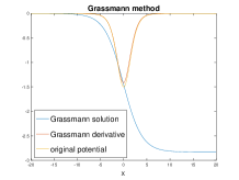
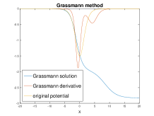
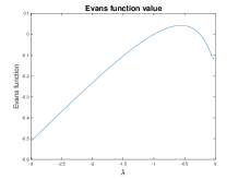
Figure 1: We plot the results from the numerical computation of the scattering and inverse scattering problems for an original reflectionless potential function ${\partial}_{x}g(0,0;x,0)=(3/2)\mathrm{sech}^{2}(x/2)$. We used the Evans function, as shown in the right panel, to determine the two discrete eigenvalues. They correspond to the zeros of the Evans function. We then constructed the corresponding scattering data function $p=p(x;0)$. We substituted this into the linear Fredholm equation which we solved numerically, to re-generate $g(0,0;x,0)$ and then ${\partial}_{x}g(0,0;x,0)$. This is shown in the left panel. The middle panel is analogous to the left panel except that we have introduced a phase shift in one of the two terms in the scattering data function $p=p(x;0)$ in order to illustrate the two distinct underlying features present.

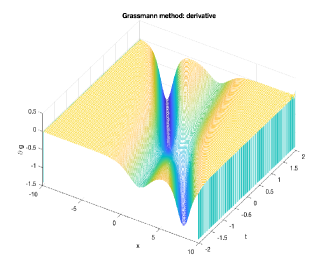
Figure 2: We plot the solution to the Korteweg–de Vries equation which demonstrates a two-soliton collision. This was achieved by assuming a suitable scattering data function form $p=p(x;t)$ with two independent exponential terms, and then numerically solving the linear Fredholm equation to generate $g(0,0;x,t)$ and then ${\partial}_{x}g(0,0;x,t)$.

We now consider numerical simulations for solutions to the scalar Korteweg–de Vries and nonlinear Schrödinger equations which are generated from given arbitrary initial scattering data $p_{0}=p_{0}(x)$ which decays in both far fields, i.e. corresponding to result (II) in Lemma 6. For each nonlinear equation we provide two independent simulations: (i) Direct numerical simulation using well-known spectral algorithms, advancing the approximate solution $u_{m}$ in successive time steps; (ii) Generating of an approximate solution $g_{\mathrm{approx}}(0,0;x,t)$ using the Grassmannian flow approach by advancing the scattering data in time to $p=p(x;t)$, and then numerically solving the linear Fredholm equation. Let us first explain the direct numerical simulation approach we employed. We chose an initial profile function $p_{0}=p_{0}(x)$ on the interval $[-L/2,L/2]$ for some fixed domain length $L>0$. In the Korteweg–de Vries case, we then numerically solved the linear Fredholm integral equation as described just above, in order to generate $g_{\mathrm{approx}}=g_{\mathrm{approx}}(0,0;x,0)$. We then set $u_{0}(x)=g_{\mathrm{approx}}(0,0;x,0)$. We chose the initial profile $p_{0}(x)=\exp(-\frac{1}{2}x^{2})\mathrm{tanh}(x/5)$ and $L=20$ in this case. The Fourier spectral method we used to advance the Korteweg–de Vries solution in time is the split-step method,

$$v_{j}=\exp(\Delta tK^{3})u_{j}\quad\text{and}\quad u_{j+1}=v_{j}+3\Delta t\mathcal{F}\bigl{(}\mathcal{F}^{-1}(v_{j})\mathcal{F}^{-1}(Kv_{j})\bigr{)}$$

where $\mathcal{F}$ denotes the Fourier transform and $K$ is the diagonal matrix of Fourier coefficients $2\pi\mathrm{i}k$. In practice we use the fast Fourier transform. We chose $\Delta t=1.5\times 10^{-3}$ and the number of Fourier modes is $2^{9}$. The result is shown in the left panel in Figure 3. In the Grassmannian flow approach, given the the initial profile $p_{0}=p_{0}(x)$ we advance the solution analytically in Fourier space to $p(x,t)=\mathcal{F}^{-1}(\exp(tK^{3})\mathcal{F}(p_{0}))$ at any given time $t\in[0,T]$, where $T=1.5$. We solve the Fredholm integral equation numerically, as described above, for $g_{\mathrm{approx}}=g_{\mathrm{approx}}(0,z;x,t)$. The solution to the Korteweg–de Vries equation at the given time $t$ is then computed as $g_{\mathrm{approx}}(0,0;x,t)$. The result is shown in the right panel in Figure 3.

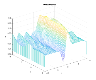
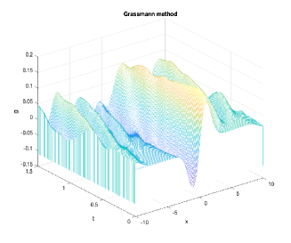
Figure 3: We plot the solution to the Korteweg–de Vries equation corresponding to the initial scattering data $p_{0}(x)=\exp(-\frac{1}{2}x^{2})\mathrm{tanh}(x/5)$. The left panel shows the evolution of the solution computed using a direct integration approach, while the right panel shows the corresponding solution computed using the Grassmannian flow approach. We also monitored the evolution of the Fredholm Determinant of $Q=Q(x,t)$ for all $x\in[-L/2,L/2]$ and it remained far from zero throughout.

In the case of the nonlinear Schrödinger equation the procedure is very similar to that for the Korteweg–de Vries equation. Given an initial scattering profile $p_{0}(x)=\frac{1}{2}\cosh(x/40)$, we restrict the interval domain to $[-L/2,L/2]$ as before. We chose $L=40$ in this case. We then numerically solve the linear Fredholm equation in order to generate $g_{\mathrm{approx}}=g_{\mathrm{approx}}(0,0;x,0)$. We use the same approximation method to solve the linear Fredholm integral equation as described above, except that we define the matrix $\widehat{Q}_{m,n}(x_{\ell};t)$ differently as follows, to account for the fact that is this case, the operator $\hat{Q}\coloneqq P^{\dagger}P$. Since we have,

$$\hat{q}(\xi,z;x,t)\coloneqq\int_{-\infty}^{0}p^{\ast}(\xi+\zeta+x;t)p(\zeta+z+x;t)\,{\mathrm{d}}\zeta,$$

we set $\tilde{P}_{m,n}(x_{\ell};t)\coloneqq p(\zeta_{m}+z_{n}+x_{\ell};t)$, and then, at any given $t\geqslant 0$ and for each $x_{\ell}$, we set $\widehat{Q}=\widehat{Q}_{m,n}(x_{\ell};t)$ to be $\widehat{Q}\coloneqq h\tilde{P}^{\dagger}\tilde{P}$. Note the $\tilde{P}^{\dagger}$ is the complex-conjugate transpose of the matrix $\tilde{P}$, and implicitly, the factor $h$ and matrix product between $\tilde{P}^{\dagger}$ and $\tilde{P}$ realise a left Riemann sum approximation of the integral in the definition of $\hat{q}$. We then solve $\widehat{P}=\widehat{G}-h\widehat{G}\widehat{Q}$ as previously. Thus, initially at $t=0$, we find $g_{\mathrm{approx}}=g_{\mathrm{approx}}(0,0;x,0)$ by using this prodcedure to generate $\widehat{G}_{m}(x_{\ell};0)$, which we then evaluate at $z_{m}=0$. We then set $u_{0}(x)=g_{\mathrm{approx}}(0,0;x,0)$. The Fourier spectral method we used to advance the nonlinear Schrödinger solution forward in time is the split-step method:

$$v_{j}=\exp(-\mathrm{i}\Delta tK^{2})u_{j}\quad\text{and}\quad u_{j+1}=v_{j}-2\mathrm{i}\Delta t\mathcal{F}\bigl{(}\bigl{(}\mathcal{F}^{-1}(v_{j})\bigr{)}^{2}\bigl{(}\mathcal{F}^{-1}(v_{j})^{\ast}\bigr{)}\bigr{)}.$$

We chose $\Delta t=0.01$ and the number of Fourier modes is $2^{8}$. The result is shown in Figure 4. In the Grassmannian flow approach, given the initial profile $p_{0}=p_{0}(x)$ we advance the solution analytically to $p(x,t)=\mathcal{F}^{-1}(\exp(-\mathrm{i}tK^{2})\mathcal{F}(p_{0}))$ for any given time $t\in[0,T]$, where $T=100$. We then use the procedure just described to generate the row vector $\widehat{G}_{m}(x_{\ell};t)$ which, again, we evaluate at $z_{m}=0$. The results are shown in Figure 4.

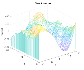
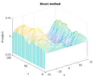
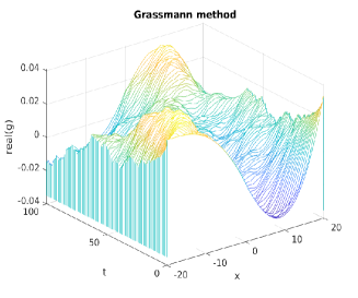
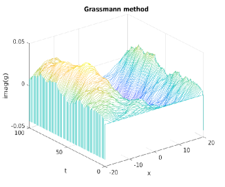
Figure 4: We plot the solution to the nonlinear Schödinger equation corresponding to the initial scattering data $p_{0}(x)=\frac{1}{2}\cosh(x/40)$. The top panels show the real and imaginary parts computed using a direct integration approach, while the bottom panels show the corresponding real and imaginary parts computed using the Grassmannian flow approach, of the solution evolution. We also monitored the evolution of the Fredholm Determinant of $Q=Q(x,t)$ for all $x\in[-L/2,L/2]$ and it remained far from zero throughout.

Remark 25 (Periodic boundary conditions)

For the numerical simulations generating Figures 3 and 4, which involved initial scattering data that decayed in both far fields, we truncated the $x$-domain from ${\mathbb{R}}$ to $[-L/2,L/2]$ for sufficiently large $L>0$. We then employed Fourier spectral methods for the direct integration methods as well as to advance the scattering data in time in the Grassmannian flow approach. This worked well as we effectively had zero, periodic boundary conditions at $x=\pm L/2$. This would obviously not be the case for exponentially growing scattering data corresponding to soliton solutions. However, that the Grassmannian flow approach carries through for periodic boundary conditions warrants further analytical investigation.

Remark 26 (Numerical inverse scattering)

Numerical techniques based on the inverse scattering transform have appeared recently. See, for example, Trogdon et al. TOD and Trogdon and Olver TO for very sophisticated and successful methods based on this approach.

Appendix B Scattering and inverse scattering problems

For completeness, we consider the scattering problem associated with potential functions $U\colon{\mathbb{R}}\to{\mathbb{C}}^{m\times m}$, for some $m\in\mathbb{N}$. Of course in our applications the function $U$ is the initial data associated with the non-commutative Korteweg–de Vries equation so for $x\in{\mathbb{R}}$:

$$U(x)\coloneqq g(0,0;x,0).$$

The scattering problem concerns determining the far-field “scatter” information associated with the eigenvalue problem for the potential function $U$ given by:

$$-{\partial}_{x}^{2}Q+UQ=\lambda Q,$$

where $\lambda$ is the spectral parameter. Note, $Q\colon{\mathbb{R}}\to{\mathbb{C}}^{m}$ is the corresponding eigenfunction $Q=Q(x,\lambda)$. We assume $U\to O_{m}$ as $|x|\to\infty$, where $O_{m}$ is the $m\times m$ zero matrix. We first determine the possible far field behaviour of the spectral problem. We set $U=O$ and denote the corresponding constant coefficient eigenvalue problem as the spatial or free eigenvalue problem. We look for solutions to the spatial eigenvalue problem of the form $Q=Q_{\infty}\mathrm{e}^{\mu x}$, where $Q_{\infty}=Q_{\infty}(\lambda)\in{\mathbb{C}}^{m}$ and we refer to the exponential growth rates $\mu=\mu(\lambda)\in{\mathbb{C}}$ as the spatial eigenvalues. We observe that such solutions exist to the spatial eigenvalue problem if and only if $\mu^{2}+\lambda=0$, repeated $m$ times. We observe the continuous spectrum, which is completely determined by the far-field spatial eigenvalue problem, coincides with the positive $\lambda$ axis. The spatial eigenvalues are given by $\mu=\pm\sqrt{-\lambda}$, each of multiplicity $m$. For convenience we set $\mu_{\pm}=\mu_{\pm}(\lambda)\in{\mathbb{C}}$ to be $\mu_{\pm}\coloneqq\pm\sqrt{-\lambda}$. The eigenspaces associated with each spatial eigenvalue $\mu_{\pm}$ have dimension $m$ and each are spanned by $\{e_{i}\colon i=1,\ldots,m\}$, where the $e_{i}\in{\mathbb{R}}^{m}$ are the vectors all of whose entries are zero except for the $i$th entry which is $1$. Hence for each spatial eigenvalue $\mu_{\pm}$ there are $n$ corresponding eigenvectors of the same exponential growth rates $\mu_{\pm}$. We collect the eigenvectors together as as columns and thus the far-field behaviour of the eigenvalue problem is summarised via the $C^{m\times m}$-valued solutions:

$$Q_{\infty}^{\pm}\coloneqq\mathrm{e}^{\mu_{\pm}x}I_{m},$$

where $I_{m}$ is the $m\times m$ identity matrix. The classical scalar case corresponds to $m=1$, and the classical development of the solution to the scattering problem can be found for example in Drazin and Johnson DJ or Keener Keener . The case $m\geqslant 1$ we consider here is a direct consequence of the standard scalar case. We define the function $\varphi\colon{\mathbb{R}}^{2}\to{\mathbb{C}}^{m\times m}$ by the following relation,

$$Q_{-\infty}(x,\lambda)=\mathrm{e}^{\mu x}\,I_{m}+\int_{-\infty}^{x}\varphi(z;x)\mathrm{e}^{\mu z}\,{\mathrm{d}}z,$$

for any $\mu$. Note that $\varphi$ does not depend on $\lambda$. In the relation, $Q_{-\infty}=Q_{-\infty}(x,\lambda)$ is the solution to the eigenvalue problem above satisfying $Q_{-\infty}\sim\mathrm{e}^{\mu x}\,I_{m}$ as $x\to-\infty$. While we know $Q_{-\infty}$ exists, we need to establish that $\varphi$ does. Substituting the relation into the eigenvalue problem, reveals, after integrating by parts twice, that $\varphi=\varphi(z;x)$ satisfies the Goursat problem,

$${\partial}_{z}^{2}\varphi-{\partial}_{x}^{2}\varphi=U\varphi\qquad\text{and}\qquad 2\frac{{\mathrm{d}}}{{\mathrm{d}}x}\varphi(x;x)=U(x),$$

where $U=U(x)$ is the given potential function, and we have assumed that $\varphi(z;x)\mathrm{e}^{\mu x}\to 0$ and ${\partial}_{z}\varphi(z;x)\mathrm{e}^{\mu x}\to 0$ as $z\to-\infty$. A solution to this problem exists, see for example, Drazin and Johnson (DJ, , p. 50) or Keener (Keener, , p. 412). Following the standard theory we consider an incident wave $Q_{+\infty}^{-}(x,\lambda)$ from $x\to+\infty$, and examine what proportions of the incident wave are, due to the presence of the potential $U$, transmitted into the opposite far field $x\to-\infty$, or reflected. We denote by $Q^{\pm}_{-\infty}=Q^{\pm}_{-\infty}(x,\lambda)$ as the respective solutions satisfying the respective asymptotic limits $Q^{\pm}_{-\infty}\sim\mathrm{e}^{\mu_{\pm}x}\,I_{m}$ as $x\to-\infty$. That we interpret the asymptotic forms $\mathrm{e}^{\mu_{\pm}x}\,I_{m}$ as incident, transmitted or reflected waves in the respective far-field limits might more readily be envisaged if we express $\mu_{\pm}(\lambda)=\pm\mathrm{i}k$ for some $k\in{\mathbb{C}}$; note that $\lambda=k^{2}$. For each $x\in{\mathbb{R}}$ and the same value of $\lambda$, the incident wave $Q_{+\infty}^{-}(x,\lambda)$ must lie in the span of $Q^{-}_{-\infty}(x,\lambda)$ and $Q^{+}_{-\infty}(x,\lambda)$. This fact amounts to the condition that there must exist constant ${\mathbb{C}}^{m\times m}$ matrix-valued coefficients $D=D(\lambda)$ and $B=B(\lambda)$, such that for every $x\in{\mathbb{R}}$:

$$Q_{+\infty}^{-}(x,\lambda)=Q^{-}_{-\infty}(x,\lambda)\,D(\lambda)+Q_{-\infty}^{+}(x,\lambda)\,B(\lambda).$$

The solution fields $Q_{+\infty}^{-}$ and $Q^{\pm}_{-\infty}$ are generated by integrating the eigenvalue problem from the respective far-field limits to some $x\in{\mathbb{R}}$. The vector fields concerned depend linearly on $\lambda$ while the data depend on $\mu_{\pm}=\pm\sqrt{-\lambda}$. We must introduce a branch cut, here along the positive $\lambda$-axis, due to the dependence on $\sqrt{-\lambda}$. The coefficients $D$ and $B$ are constructed from such solution fields. We show how this is achieved in practice via the Evans function in Appendix C. Both coefficients thus depend similarly on $\lambda$ and $\sqrt{-\lambda}$. However we set $\lambda=k^{2}$ with $k\in{\mathbb{C}}$, thus unravelling the two Riemann surfaces associated with $\sqrt{-\lambda}$, mapping them both to the upper and lower halves of the $k$-complex plane. Consequently the maps $k\mapsto D(k^{2})$ and $k\mapsto B(k^{2})$ are analytic. We now subsitute the corresponding expressions for $Q_{-\infty}^{\pm}=Q_{-\infty}^{\pm}(x;\lambda)$ in terms of $\varphi$ from the relation above using $\lambda=k^{2}$. Assuming $\varphi(z;x)=0$ for $z>x$, that $\mu_{\pm}=\pm\mathrm{i}k$ and rearranging, this compatability condition involving $D$ and $B$ generates the following relation:

$$\int_{-\infty}^{+\infty}\varphi(z;x)\mathrm{e}^{-\mathrm{i}kz}\,{\mathrm{d}}z= \;Q_{+\infty}^{-}(x,k^{2})D^{-1}(\lambda)-\mathrm{e}^{-\mathrm{i}kx}I_{m}-\mathrm{e}^{\mathrm{i}kx}B(k^{2})D^{-1}(k^{2})$$

$$\;-\int_{-\infty}^{+\infty}\varphi(z;x)\mathrm{e}^{\mathrm{i}kz}\,{\mathrm{d}}z\,B(k^{2})D^{-1}(k^{2}).$$

While $D(k^{2})$ and thus $\det\bigl{(}D(k^{2})\bigr{)}$ is analytic in $k\in{\mathbb{C}}$, the determinant $\det\bigl{(}D(k^{2})\bigr{)}$ may have zeros. These zeros coincide precisely with discrete eigenvalues and thus bound states of the underlying eigenvalue problem—see Appendix C for a discussion on this. Suppose we define the function $\hat{D}=\hat{D}(\lambda)$ by the relation $D(\lambda)=I_{m}+\hat{D}(\lambda)$. Let $\nu\colon{\mathbb{C}}^{m\times m}\to{\mathbb{C}}^{m\times m}$ denote the function $\nu(\hat{D})\coloneqq-\hat{D}(I_{m}+\hat{D})^{-1}\det(I_{m}+\hat{D})$. Then $\nu\colon{\mathbb{C}}^{m\times m}\to{\mathbb{C}}^{m\times m}$ is an analytic function; see Simon (Simon:Traces, , p. 46). Hence we observe that $D^{-1}(\lambda)=I_{m}+\nu\bigl{(}(\hat{D}(\lambda)\bigr{)}/\det\bigl{(}I_{m}+\hat{D}(\lambda)\bigr{)}$, and so the singularites of $D^{-1}=D^{-1}(\lambda)$ correspond to the zeros of $\det\bigl{(}D(\lambda)\bigr{)}$. Furthermore, if we assume the potential function $U=U(x)$ is bounded then we know the discrete spectrum remains in a bounded region of the complex $\lambda$-plane. To see this we observe, by direct computation from the eigenvalue problem, we have

$$|\lambda|\,\|Q\|_{L^{2}({\mathbb{R}};{\mathbb{C}}^{m\times m})}^{2}\leqslant\|{\partial}Q\|_{L^{2}({\mathbb{R}};{\mathbb{C}}^{m\times m})}^{2}+\|U\|_{L^{\infty}({\mathbb{R}};{\mathbb{C}}^{m\times m})}\|Q\|_{L^{2}({\mathbb{R}};{\mathbb{C}}^{m\times m})}^{2}.$$

Hence we observe that if we restrict ourselves to $H^{1}({\mathbb{R}};{\mathbb{C}}^{m\times m})$-valued eigenfunctions, which we do, then any discrete eigenvalues $\lambda$ are necessarily bounded in magnitude.

Now consider the contour in the complex $k$-plane given by $\mathcal{C}\coloneqq\{k\in{\mathbb{C}}\colon k=\kappa-\mathrm{i}\gamma,~{}\kappa\in{\mathbb{R}}\}$ for some fixed real constant $\gamma>0$ sufficiently large so that all the poles of $D^{-1}(\lambda)$ lie above $\mathcal{C}$. Define the function $F\colon{\mathbb{R}}\to{\mathbb{C}}^{m\times m}$ by the following contour integral, which is well defined by our choice of the contour $\mathcal{C}$:

$$F(Z)\coloneqq\frac{1}{2\pi}\int_{\mathcal{C}}B(k^{2})D^{-1}(k^{2})\mathrm{e}^{\mathrm{i}kZ}\,{\mathrm{d}}k.$$

Multiplying both sides of the integral relation just above for $\varphi=\varphi(z;x)$ by $\mathrm{e}^{\mathrm{i}k\xi}$, integrating along the contour $\mathcal{C}$ and dividing through by $2\pi$, we find that $\varphi$ must satisfy:

$$\varphi(\xi;x)=\frac{1}{2\pi}\int_{\mathcal{C}}Q_{+\infty}^{-}(x,k^{2})D^{-1}(k^{2})\mathrm{e}^{\mathrm{i}k\xi}\,{\mathrm{d}}k-F(\xi+x)-\int_{-\infty}^{+\infty}\varphi(z;x)F(z+\xi)\,{\mathrm{d}}z.$$

Note by standard anaylsis the integral of $\mathrm{e}^{\mathrm{i}k(\xi-x)}$ along the contour $\mathcal{C}$ is zero. Indeed the first contour integral on the right above is also zero, as follows. Approximate the contour integral by truncating the contour $\mathcal{C}$ so that $\kappa\in[-R,R]$ for some large $R>0$. Call the truncated contour $\mathcal{C}_{R}$. Construct a closed contour by appending a semi-circular arc $\mathcal{C}_{\mathrm{arc}}$ of radius $R$ to $\mathcal{C}_{R}$; so the ends of $\mathcal{C}_{\mathrm{arc}}$ coincide with the ends of $\mathcal{C}_{R}$, and the lowest point of $\mathcal{C}_{\mathrm{arc}}$ lies at $k=-\gamma-R$. By Cauchy’s Theorem, since the argument is analytic inside $\mathcal{C}_{R}+\mathcal{C}_{\mathrm{arc}}$, the integral is zero. We then take the limit $R\to\infty$. Jordan’s Lemma implies the integral along $\mathcal{C}_{\mathrm{arc}}$ is zero provided $\xi<x$; see Remark 28 below. Hence the integral along $\mathcal{C}$ is zero. Consequently we see that $\varphi$ must satisfy:

$$F(\xi+x)+\varphi(\xi;x)+\int_{-\infty}^{x}\varphi(z;x)F(z+\xi)\,{\mathrm{d}}z=0.$$

Let us now examine how to evaluate the scattering data $F=F(Z)$. As we have just seen, again we approximate the contour integral by truncating the contour $\mathcal{C}$ so that $\kappa\in[-R,R]$ for some large $R>0$, and call the truncated contour $\mathcal{C}_{R}$. Then we construct a closed contour consisting of the interval $[+R,-R]$ on the real $k$-axis, noting the direction of integration indicated, the contour $\mathcal{C}_{R}$, and the two straight-line contours $\mathcal{C}_{1}$ and $\mathcal{C}_{2}$, respectively from $k=R-\mathrm{i}\gamma$ to $k=R$, and from $k=-R$ to $k=-R-\mathrm{i}\gamma$. By residue calculus, the integral around the closed contour $\mathcal{C}_{R}\cup\mathcal{C}_{1}\cup[+R,-R]\cup\mathcal{C}_{2}$ is given by $2\pi\mathrm{i}$ times the sum of the residues of $B(k^{2})D^{-1}(k^{2})\mathrm{e}^{\mathrm{i}kZ}$ at the zeros $k=k_{n}$ of $\det\bigl{(}D(k^{2})\bigr{)}=0$. In the large $R$ limit the contour integrals along $\mathcal{C}_{1}$ and $\mathcal{C}_{2}$ vanish and we are left with

$$F(Z)=\frac{1}{2\pi}\int_{-\infty}^{+\infty}B(k^{2})D^{-1}(k^{2})\mathrm{e}^{\mathrm{i}kZ}\,{\mathrm{d}}k+\mathrm{i}\sum_{n}\mathrm{res}\bigl{(}B(k^{2})D^{-1}(k^{2})\mathrm{e}^{\mathrm{i}kZ}\colon k=k_{n}\bigr{)}.$$

The zeros $\det\bigl{(}D(k^{2})\bigr{)}$ of concern here, within the closed contour, occur at $k_{n}=-\mathrm{i}\sqrt{|\lambda_{n}|}$. By Taylor series expansion about any zero $k=k_{n}$ we observe, $D(k^{2})=\bigl{(}D^{\prime}(k_{n}^{2})\,(2k_{n})\bigr{)}(k-k_{n})+\mathcal{O}\bigl{(}|k-k_{n}|^{2}\bigr{)}$ and so

$$\mathrm{res}\bigl{(}B(k^{2})D^{-1}(k^{2})\mathrm{e}^{\mathrm{i}kZ}\colon k=k_{n}\bigr{)}=-\tfrac{1}{2}\frac{B(\lambda_{n})}{D^{\prime}(\lambda_{n})}\frac{\mathrm{e}^{\sqrt{|\lambda_{n}|}Z}}{\sqrt{|\lambda_{n}|}}.$$

Hence the scattering data $F=F(Z)$ is given by

$$F(Z)=\frac{1}{2\pi}\int_{-\infty}^{+\infty}B(k^{2})D^{-1}(k^{2})\mathrm{e}^{\mathrm{i}kZ}\,{\mathrm{d}}k-\tfrac{1}{2}\sum_{n}\frac{B(\lambda_{n})}{D^{\prime}(\lambda_{n})}\frac{\mathrm{e}^{\sqrt{|\lambda_{n}|}Z}}{\sqrt{|\lambda_{n}|}}.$$

Note in particular that the contribution to the scattering data $F=F(Z)$ from the discrete spectra $\lambda=\lambda_{n}$ grows exponentially in the limit $Z\to+\infty$. In summary therefore, we see that $\varphi=\varphi(\xi;x)$ necessarily satisfies the linear Volterra integral equation involving the scattering data $F=F(\xi+x)$ shown, with $F=F(Z)$ given by the formula just above. The linear Volterra integral equation is the Gel’fand–Levitin–Marchenko equation. If we combine this knowledge with the observation that we can resconstruct the original potential function $U$ from $\varphi(x,x)$, via the boundary relation in the Goursat problem above, we have thus also completed the formulation of the inverse scattering problem. In other words, given the data implicit in the function $F=F(Z)$, the eigenvalues and transmission and reflection coefficients, we can then, in principle, solve the Gel’fand–Levitin–Marchenko equation for $\varphi$, and evaluate $U$.

Remark 27 (Relation to the linear Fredholm kernel equation)

The relation between the version of the Gel’fand–Levitin–Marchenko equation for $\varphi=\varphi(Z;X)$ above, given by,

$$F(Z+X)+\varphi(Z;X)+\int_{-\infty}^{X}\varphi(Y;X)F(Y+Z)\,{\mathrm{d}}Y=0,$$

and the linear Fredholm equation for the kernel $\hat{g}(z;x)=g(0,z;x)$ given by (suppressing any time-dependence for the moment),

$$p(z+x)=\hat{g}(z;x)-\int_{-\infty}^{0}\hat{g}(\eta;x)p(\eta+z+x)\,{\mathrm{d}}\eta,$$

is given as follows. Making the change of variables $z\coloneqq Z-\frac{1}{2}x$, $\eta\coloneqq Y-\frac{1}{2}x$ and then $x\coloneqq 2X$ in the linear Fredholm kernel equation, we arrive at the relation:

$$p(Z+X)=\hat{g}(Z-X;2X)-\int_{-\infty}^{X}\hat{g}(Y-X;2X)p(Y+Z)\,{\mathrm{d}}Y.$$

We then see that if we identify $\varphi(Z;X)\coloneqq g(z;x)\equiv g(Z-X;2X)$ and $F(Z+X)\coloneqq-p(x+z)\equiv-p(Z+X)$, then $\varphi(Z;X)$ satisfies the Gel’fand–Levitin–Marchenko equation above.

Remark 28

By rescaling and iteration it can be shown that $Q\mathrm{e}^{\mathrm{i}kx}=1+\tilde{Q}$, where $\tilde{Q}=\mathcal{O}(|k|^{-2})$ as $|k|\to\infty$. Hence we see that,

$$\frac{1}{2\pi}\int_{\mathcal{C}_{\mathrm{arc}}}Q_{+\infty}^{-}(x,k^{2})D^{-1}(k^{2})\mathrm{e}^{\mathrm{i}k\xi}\,{\mathrm{d}}k =\frac{1}{2\pi}\int_{\mathcal{C}_{\mathrm{arc}}}Q_{+\infty}^{-}(x,k^{2})\mathrm{e}^{\mathrm{i}kx}D^{-1}(k^{2})\mathrm{e}^{\mathrm{i}k(\xi-x)}\,{\mathrm{d}}k$$

$$=\delta(\xi-x)+\frac{1}{2\pi}\int_{\mathcal{C}_{\mathrm{arc}}}\tilde{Q}(x,k^{2})D^{-1}(k^{2})\mathrm{e}^{\mathrm{i}k(\xi-x)}\,{\mathrm{d}}k,$$

which is zero provided $\xi<x$ by Jordan’s Lemma.

Appendix C Computing the transmission and reflection coefficients

Recall the scattering problem outlined at the beginning of Appendix B. We outline herein a practical approach to determine the scattering data coefficients $D=D(\lambda)$ and $B=B(\lambda)$ associated with the scattering spectral problem for given potential functions $U=U(x)$. The shooting and matching technique that underlies the Evans function method is ideally suited to this purpose. See Alexander et al. AGJ90 for a comprehensive account of the Evans function, and indeed, the Grassmaninnian determinent bundle that underlies it. To begin, we largely shadow the development in the first part of Appendix B, albeit for the eigenvalue problem re-written in the following form. If we set $P=P(x,\lambda)\in{\mathbb{C}}^{m}$ to be $P\coloneqq{\partial}_{x}Q$, then we observe that the eigenvalue problem can be re-written as the first order system

$$\frac{{\mathrm{d}}Y}{{\mathrm{d}}x}=AY,\qquad\text{where}\quad Y\coloneqq\begin{pmatrix}Q\\ P\end{pmatrix}\quad\text{and}\quad A(x,\lambda)\coloneqq\begin{pmatrix}O_{m}&I_{m}\\ U-\lambda I_{m}&O_{m}\end{pmatrix}.$$

Associated with this first order system is the adjoint system for $Z=Z(x,\lambda)\in{\mathbb{C}}^{1\times 2m}$ given by

$$\frac{{\mathrm{d}}Z}{{\mathrm{d}}x}=-ZA.$$

We observe that $({\mathrm{d}}/{\mathrm{d}}x)(ZY)=0$ and so $ZY$ is constant and independent of $x\in{\mathbb{R}}$. Let $Y_{-\infty}^{\pm}=Y_{-\infty}^{\pm}(x,\lambda)$ and $Y_{+\infty}^{-}=Y_{+\infty}^{-}(x,\lambda)$ denote the $C^{2m\times m}$ matrices of solutions with the far-field aymptotic behaviour,

$$Y_{-\infty}^{\pm}(x,\lambda)\sim\begin{pmatrix}I_{m}\\ \mu_{\pm}I_{m}\end{pmatrix}\mathrm{e}^{\mu_{\pm}x}~{}\text{as}~{}x\to-\infty\quad\text{and}\quad Y_{+\infty}^{-}(x,\lambda)\sim\begin{pmatrix}I_{m}\\ \mu_{-}I_{m}\end{pmatrix}\mathrm{e}^{\mu_{-}x}~{}\text{as}~{}x\to+\infty.$$

These are just the augmented versions (with the field block $P$ appended) of the corresponding respective fields $Q_{-\infty}^{\pm}=Q_{-\infty}^{\pm}(x,\lambda)$ and $Q_{+\infty}^{-}=Q_{+\infty}^{-}(x,\lambda)$ from Appendix B. The matching condition that for each $x\in{\mathbb{R}}$ the field $Y_{+\infty}^{-}$ must lie in the span of $Y_{+\infty}^{-}$ and $Y_{-\infty}^{+}$ applies precisely as before (though now augmented to include the block $P$) and thus there must exist constant ${\mathbb{C}}^{m\times m}$ matrix-valued coefficients $D=D(\lambda)$ and $B=B(\lambda)$, such that for every $x\in{\mathbb{R}}$:

$$Y_{+\infty}^{-}(x,\lambda)=Y^{-}_{-\infty}(x,\lambda)\,D(\lambda)+Y^{+}_{-\infty}(x,\lambda)\,B(\lambda).$$

Now suppose $Z_{-\infty}^{\pm}=Z_{-\infty}^{\pm}(x,\lambda)$ are the $C^{m\times 2m}$ block solutions to the adjoint problem with the far-field aymptotic behaviour,

$$Z_{-\infty}^{\pm}(x,\lambda)\sim\begin{pmatrix}-\mu_{\pm}I_{m}&I_{m}\end{pmatrix}\mathrm{e}^{\mu_{\pm}x}~{}\text{as}~{}x\to-\infty.$$

The asymptotic solutions shown are the solutions to the adjoint problem in the far-field. Naturally for these block solutions we know $({\mathrm{d}}/{\mathrm{d}}x)(ZY)=O_{m}$ and so $ZY$ is constant. However we note that for each $\lambda\in{\mathbb{C}}$ the far field eigenvectors satisfy,

$$\begin{pmatrix}-\mu_{\pm}I_{m}&I_{m}\end{pmatrix}\begin{pmatrix}I_{m}\\ \mu_{\pm}I_{m}\end{pmatrix}=O_{m},$$

which implies $Z_{-\infty}^{\pm}(-\infty,\lambda)Y_{-\infty}^{\pm}(-\infty,\lambda)=O_{m}$, which in turn implies $Z_{-\infty}^{\pm}(x,\lambda)Y_{-\infty}^{\pm}(x,\lambda)=O_{m}$, for each $x\in{\mathbb{R}}$. The latter conclusion follows from the fact that $ZY$ is constant on ${\mathbb{R}}$. Similarly we observe that,

$$\begin{pmatrix}-\mu_{\pm}I_{m}&I_{m}\end{pmatrix}\begin{pmatrix}I_{m}\\ \mu_{\mp}I_{m}\end{pmatrix}=\pm(\mu_{-}-\mu_{+})I_{m},$$

which implies $Z_{-\infty}^{\pm}(-\infty,\lambda)Y_{-\infty}^{\mp}(-\infty,\lambda)=\pm(\mu_{-}-\mu_{+})I_{m}$, which in turn implies that for each $x\in{\mathbb{R}}$, $Z_{-\infty}^{\pm}(x,\lambda)Y_{-\infty}^{\mp}(x,\lambda)=\pm(\mu_{-}-\mu_{+})I_{m}$. Consequently if we respectively pre-multiply the compatability condition by $Z_{-\infty}^{+}(x,\lambda)$ and then $Z_{-\infty}^{-}(x,\lambda)$, we observe that the coefficient matrices $D=D(\lambda)$ and $B=B(\lambda)$ are given by:

$$D(\lambda)=(\mu_{-}-\mu_{+})^{-1}Z_{-\infty}^{+}(x,\lambda)Y_{+\infty}^{-}(x,\lambda)\quad\text{and}\quad B(\lambda)=(\mu_{+}-\mu_{-})^{-1}Z_{-\infty}^{-}(x,\lambda)Y_{+\infty}^{-}(x,\lambda).$$

Note the quantities on the right are independent of $x\in{\mathbb{R}}$. Eigenvalues of the original spectral problem for $Q=Q(x,\lambda)$, or equivalently for the problem for $Y=Y(x,\lambda)$ above correspond to solutions that decay in both far-fields. In particular the far-field solutions are not oscillatory, so occur for $\lambda<0$, away from the continuous spectrum. Further, for $\lambda<0$ the solution $Y^{-}_{+\infty}=Y_{+\infty}^{-}(x,\lambda)$, by construction, decays exponentially like $\mathrm{e}^{\mu_{-}x}$ as $x\to+\infty$, where recall $\mu_{-}(\lambda)=-\sqrt{-\lambda}$. For $Y^{-}_{+\infty}=Y_{+\infty}^{-}(x,\lambda)$ to be an eigenfunction it must lie in the span of the solutions $Y_{-\infty}^{+}=Y_{-\infty}^{+}(x,\lambda)$, and the condition for this to hold is that: $\det\bigl{(}D(\lambda)\bigr{)}=0$, i.e. eigenvalues $\lambda$ coincide with zeroes of the determinant of the coefficient matrix $D=D(\lambda)$.

Remark 29 (Practical computation)

In practice when integrating the eigenvalue problem to determine $Y^{\pm}_{-\infty}=Y_{-\infty}^{\pm}(x,\lambda)$ and $Y^{-}_{+\infty}=Y_{+\infty}^{-}(x,\lambda)$ it is preferable to avoid the exponential behaviour in the far-field. We can achieve this by setting $\hat{Y}^{\pm}_{-\infty}\coloneqq Y_{-\infty}^{\pm}\mathrm{e}^{-\mu_{\pm}x}$ and $\hat{Y}^{-}_{+\infty}\coloneqq Y_{+\infty}^{-}\mathrm{e}^{-\mu_{-}x}$ as well as $\hat{Z}^{\pm}_{-\infty}\coloneqq Z_{-\infty}^{\pm}\mathrm{e}^{-\mu_{\pm}x}$. The respective rescaled solutions $\hat{Y}=Y\mathrm{e}^{-\mu x}$ and $\hat{Z}=Z\mathrm{e}^{-\mu x}$ satisfy the equations

$$\frac{{\mathrm{d}}\hat{Y}}{{\mathrm{d}}x}=(A-\mu I_{2m})\hat{Y}\qquad\text{and}\qquad\frac{{\mathrm{d}}\hat{Z}}{{\mathrm{d}}x}=-\hat{Z}(A+\mu I_{2m}).$$

and $\hat{Y}$ as well as $\hat{Z}$ have constant far-field limiting behaviours—the same as those for $Y$ and $Z$ but without the exponential factors. Since $\mu_{-}=-\mu_{+}$ it is evident that

$$D(\lambda) =(\mu_{-}-\mu_{+})^{-1}\hat{Z}_{-\infty}^{+}(x,\lambda)\hat{Y}_{+\infty}^{-}(x,\lambda),$$

$$B(\lambda) =(\mu_{+}-\mu_{-})^{-1}\hat{Z}_{-\infty}^{-}(x,\lambda)\hat{Y}_{+\infty}^{-}(x,\lambda)\,\mathrm{e}^{2\mu_{-}x}.$$

In the latter case, since $ZY$ is constant and we can evaluate the right-hand side at any value $x\in{\mathbb{R}}$, we can deal with the problematic exponential factor by evaluating $B=B(\lambda)$ at $x=0$.

Remark 30

To evaluate the scattering data $F=F(Z)$ in the Gel’fand–Levitan–Marchenko equation, or equivalently $p=p(Z)$ in the linear Fredholm kernel equation, associated with a given potential $U$, we need to determine $D^{\prime}(\lambda)$; see Appendix B. By differentiating the formula for $D=D(\lambda)$ in Remark 29, we observe

$$D^{\prime}(\lambda)= \;\Bigl{(}{\partial}_{\lambda}\bigl{(}(\mu_{-}-\mu_{+})^{-1}\bigr{)}\Bigr{)}\hat{Z}_{-\infty}^{+}(x,\lambda)\hat{Y}_{+\infty}^{-}(x,\lambda)$$

$$\;+(\mu_{-}-\mu_{+})^{-1}\bigl{(}{\partial}_{\lambda}\hat{Z}_{-\infty}^{+}(x,\lambda)\bigr{)}\hat{Y}_{+\infty}^{-}(x,\lambda)$$

$$\;+(\mu_{-}-\mu_{+})^{-1}\hat{Z}_{-\infty}^{+}(x,\lambda)\bigl{(}{\partial}_{\lambda}\hat{Y}_{+\infty}^{-}(x,\lambda)\bigr{)}.$$

By direct computation ${\partial}_{\lambda}\mu_{\pm}=-1/(2\mu_{\pm})$ and so ${\partial}_{\lambda}\bigl{(}(\mu_{-}-\mu_{+})^{-1}\bigr{)}=\tfrac{1}{2}(\mu_{-}-\mu_{+})^{-1}(\mu_{-}\mu_{+})^{-1}$. The quantity ${\partial}_{\lambda}\hat{Y}$ satisfies the linear flow equation

$$\frac{{\mathrm{d}}{\partial}_{\lambda}\hat{Y}}{{\mathrm{d}}x}=\bigl{(}-\mu^{\prime}(\lambda)I_{2m}-\hat{J}_{2m}\bigr{)}\hat{Y}+(A-\mu I_{2m}){\partial}_{\lambda}\hat{Y},$$

where $\hat{J}_{2m}$ is the matrix of four $m\times m$ blocks, all of which are $O_{m}$ except for the lower left block which is $I_{m}$. An analogous flow equation exists for ${\partial}_{\lambda}\hat{Z}$. The linear flow equations for ${\partial}_{\lambda}\hat{Y}$ and ${\partial}_{\lambda}\hat{Z}$ can be integrated alongside those for $\hat{Y}$ and $\hat{Z}$ to construct $D=D(\lambda)$ and $D^{\prime}=D^{\prime}(\lambda)$.

The determinant $\det\bigl{(}D(\lambda)\bigr{)}$ is well-known as the Evans function or miss-distance function; see for example Alexander et al. AGJ90 . The Evans function has several equivalent formulations; see for example Karambal and Malham KM . Above it is defined in terms a transmission coefficient. However its equivalent classical definition is:

$$\det\bigl{(}D(\lambda)\bigr{)}\coloneqq\mathrm{e}^{-\int_{0}^{x}\mathrm{tr}\bigl{(}A(x,\lambda)\bigr{)}\,{\mathrm{d}}x}\det\bigl{(}Y_{-\infty}^{+}(x,\lambda)\,\,Y_{+\infty}^{-}(x,\lambda)\bigr{)},$$

where $Y_{-\infty}^{+}=Y_{-\infty}^{+}(x,\lambda)$ and $Y_{+\infty}^{-}=Y_{+\infty}^{-}(x,\lambda)$ are the block solutions identified above.

Remark 31 (Practical eigenfunction normalisation)

An alternative stable approach in the scalar case to determining the normalisation factors associated with the functions $\mathrm{e}^{\sqrt{\lambda_{n}}Z}$ in the discrete spectrum sum in $F(Z)$, is as follows. Simply append a third component onto the integration of $Y^{\pm}_{-\infty}$, whose vector field is given by the square of the first component—recall the discrete eigenvalues and eigenfunctions are real here. Then when integrating the appended set of ordinary differential equations from $x\to-\infty$ to the opposite far field, the third component gives the square integral of the eigenfunction. We then normalise using the reciprocal.

Remark 32

We note that the expression for the potential function $U(x)=2({\mathrm{d}}/{\mathrm{d}}x)\varphi(x;x)$ exhibits a sign difference to the corresponding expression $U(X)=-2({\mathrm{d}}/{\mathrm{d}}X)K(X,X)$ given in Remark 15. That these two expressions do match can be established once we take into account both the transformations indicated in Remark 15 in Secion 5, and that indicated in Remark 27 in Appendix B.

Remark 33 (Scatter Grassmannians and superpotentials)

The Evans function can be applied to more general eigenvalue problems, including examples where the potential matrix $U$ entries are not necessarily zero in the far field, or for non-selfadjoint eigenvalue problems, and so forth. In such cases the matrix $A$ may have a more general form than that indicated above, and the far field limits of the columns of $Y_{-\infty}^{+}=Y_{-\infty}^{+}(x,\lambda)$ and $Y_{+\infty}^{-}=Y_{+\infty}^{-}(x,\lambda)$ may be different with different exponential rates. To evaluate the Evans function, the typical procedure is to integrate $Y_{-\infty}^{+}$ and $Y_{+\infty}^{-}$ from the far-field to $x=0$ and evaulate $\det\bigl{(}D(\lambda)\bigr{)}$ at $x=0$. Remark 29 showed how to deal with far-field behaviour with a single exponential rate. However numerically, multiple distinct exponential growth rates represent a ‘stiff’ numerical integration problem. One natural solution is to integrate the linear differential equation for $Y$ by continuous orthogonalisation; see Humpherys and Zumbrun HZ . Another natural approach is project the Stiefel manifold frames $Y_{-\infty}^{+}\in{\mathbb{C}}^{2m\times k}$ and $Y_{+\infty}^{-}\in{\mathbb{C}}^{2m\times(2m-k)}$ onto the respective Grassmannians $\mathrm{Gr}({\mathbb{C}}^{2m};{\mathbb{C}}^{k})$ and $\mathrm{Gr}({\mathbb{C}}^{2m};{\mathbb{C}}^{2m-k})$. Note in the more general context the dimensions of the stable manifolds in the far-fields do not necessarily match, though away from the essential spectrum, they do add to $2m$. Here, we assign one as having dimension $1\leqslant k<2m$. In this context we denote these Grassmann manifolds as scattering Grassmannians. As homogeneous manifolds, the exponential growth rates present in the solution frames in the far-field, do not play a role on the corresponding Grassmannians—though are present in the group $\mathrm{GL}({\mathbb{C}}^{k})$ flow through the fibres if we view, say, the Grassmannian $\mathrm{Gr}({\mathbb{C}}^{2m};{\mathbb{C}}^{k})$ as the base space in the Stiefel manifold principle fibre bundle $\pi\colon\mathrm{St}({\mathbb{C}}^{2m},k)\to\mathrm{Gr}({\mathbb{C}}^{2m};{\mathbb{C}}^{k})$. However, for a fixed $\lambda\in{\mathbb{C}}$, when integrating on the Grassmannian $\mathrm{Gr}({\mathbb{C}}^{2m};{\mathbb{C}}^{k})$ from one far field to the opposite using a given coordinate patch/cell which, say, is parameterised by $G\in{\mathbb{C}}^{(2m-k)\times k}$, the entries in $G$ may become singular at particular values of $x\in{\mathbb{R}}$. This is naturally circumvented by changing coordinate patches; see for example Ledoux et al. LMT . Also see Pressley and Segal (PS, , Sec. 8.12). In the case of self-adjoint spectral problems, these singularities for $(\lambda,x)\in{\mathbb{R}}^{2}$, indicate potential eigenvalues and contribute to the Maslov index. See Beck and Malham BM for more details. Further, suppose the eigenvalue problem (not necessarily self-adjoint) has the form

$$\frac{{\mathrm{d}}Y}{{\mathrm{d}}x}=A\,Y,\quad\text{where}\quad Y\coloneqq\begin{pmatrix}Q\\ P\end{pmatrix}\quad\text{and}\quad A\coloneqq\begin{pmatrix}a&b\\ c&d\end{pmatrix},$$

with $x\in{\mathbb{R}}$ and the the commensurate block matrices $a$, $b$, $c$ and $d$ may all depend on $x\in{\mathbb{R}}$ and a spectral parameter $\lambda\in{\mathbb{C}}$. Then the maps $G\colon Q\mapsto P$ and $G^{\prime}\colon O\mapsto Q$, assuming they exist, satisfy the respective Riccati equations ${\mathrm{d}}G/{\mathrm{d}}x=c+dG-G(a+bG)$ and ${\mathrm{d}}G^{\prime}/{\mathrm{d}}x=b+aG^{\prime}-G^{\prime}(d+cG^{\prime})$. The solutions $G$ and $G^{\prime}$ represent superpotentials; see Bougie et al. BGMR . Formally, the fields $G$ and $G^{\prime}$ can be used to diagonalise ${\mathrm{d}}/{\mathrm{d}}x-A$ in the sense that

$$\begin{pmatrix}{\mathrm{id}}&G^{\prime}\\ G&{\mathrm{id}}\end{pmatrix}^{-1}\begin{pmatrix}{\mathrm{d}}/{\mathrm{d}}x-A\end{pmatrix}\begin{pmatrix}{\mathrm{id}}&G^{\prime}\\ G&{\mathrm{id}}\end{pmatrix}=\begin{pmatrix}{\mathrm{d}}/{\mathrm{d}}x-(a+bG)&O\\ O&{\mathrm{d}}/{\mathrm{d}}x-(d+cG^{\prime})\end{pmatrix}.$$

Note, for example, the field ${\mathrm{d}}/{\mathrm{d}}x-(a+bG)$ generates the flow through the fibres of the principle fibre bundle $\pi\colon\mathrm{St}({\mathbb{C}}^{2m},{\mathbb{C}}^{k})\to\mathrm{Gr}({\mathbb{C}}^{2m};{\mathbb{C}}^{k})$, i.e. $Q=Q(x,\lambda)$ satisfies ${\mathrm{d}}Q/{\mathrm{d}}x=(a+bG)Q$ in the chosen coordinate patch indicated. See Ledoux et al. LMT and Remark 4. The superpotential fields can be used to analytically generate eigenvalues and eigenfunctions associated with certain potentials, such as the ‘$\mathrm{sech}^{2}$’-potential. For more details, see Bougie et al. BGMR and also Keener (Keener, , p. 323).