Modelling Instance-Level Annotator Reliability for Natural Language Labelling Tasks

Abstract

When constructing models that learn from noisy labels produced by multiple annotators, it is important to accurately estimate the reliability of annotators. Annotators may provide labels of inconsistent quality due to their varying expertise and reliability in a domain. Previous studies have mostly focused on estimating each annotator’s overall reliability on the entire annotation task. However, in practice, the reliability of an annotator may depend on each specific instance. Only a limited number of studies have investigated modelling per-instance reliability and these only considered binary labels. In this paper, we propose an unsupervised model which can handle both binary and multi-class labels. It can automatically estimate the per-instance reliability of each annotator and the correct label for each instance. We specify our model as a probabilistic model which incorporates neural networks to model the dependency between latent variables and instances. For evaluation, the proposed method is applied to both synthetic and real data, including two labelling tasks: text classification and textual entailment. Experimental results demonstrate our novel method can not only accurately estimate the reliability of annotators across different instances, but also achieve superior performance in predicting the correct labels and detecting the least reliable annotators compared to state-of-the-art baselines.

1 Introduction

In many natural language processing (NLP) applications, the performance of supervised machine learning models depends on the quality of the corpus used to train the model. Traditionally, labels are collected from multiple annotators/experts who are assumed to provide reliable labels. However, in reality, these experts may have varying levels of expertise depending on the domains, and thus may disagree on labelling in certain cases Aroyo and Welty (2013). A rapid and cost-effective alternative is to obtain labels through crowdsourcing Snow et al. (2008); Poesio et al. (2013, 2017). In crowdsourcing, each instance is presented to multiple expert or non-expert annotators for labelling. However, labels collected in this manner could be noisy, since some annotators could produce a significant number of incorrect labels. This may be due to differing levels of expertise, lack of financial incentive and interest Poesio et al. (2017), as well as the tedious and repetitive nature of the annotation task Raykar et al. (2010); Bonald and Combes (2017).

Thus, in order to ensure the accuracy of the labelling and the quality of the corpus, it is crucial to estimate the reliability of the annotators automatically without human intervention.

Previous studies have mostly focused on evaluating the annotators’ overall reliability Gurevych and Kim (2013); Sheshadri and Lease (2013); Poesio et al. (2017). Measuring the reliability on a per-instance basis is however useful as we may expect certain annotators to have more expertise in one domain than another, and as a consequence certain annotation decisions will be more difficult than others. This resolves a potential issue of models that only assign an overall reliability to each annotator, where such a model would determine an annotator with expertise in a single domain to be unreliable for the model, even though the annotations are reliable within the annotator’s domain of expertise.

Estimating per-instance reliability is also helpful for unreliable annotator detection and task allocation in crowdsourcing, where the cost of labelling data is reduced using proactive learning strategies for pairing instances with the most cost-effective annotators Donmez and Carbonell (2008); Li et al. (2017). Although reliability estimation has been studied for a long time, only a limited number of studies have examined how to model the reliability of each annotator on a per-instance basis. Additionally, these in turn have only considered binary labels  Yan et al. (2010, 2014); Wang and Bi (2017), and cannot be extended to multi-class classification in a straightforward manner.

In order to handle both binary and multi-class labels, our approach extends one of the most popular probabilistic models for label aggregation, proposed by Hovy et al. Hovy et al. (2013). One challenge of extending the model is the definition of the label and reliability probability distributions on a per-instance basis. Our approach introduces a classifier which predicts the correct label of an instance, and a reliability estimator, providing the probability that an annotator will label a given instance correctly. The approach allows us to simultaneously estimate the per-instance reliability of the annotators and the correct labels, allowing the two processes to inform each other. Another challenge is to select appropriate training methods to learn a model with high and stable performance. We investigate training our model using the EM algorithm and cross entropy. For evaluation, we apply our method to six datasets including both synthetic and real-world datasets (see Section 4.1). In addition, we also investigate the effect on the performance when using different text representation methods and text classification models (see Section 4.2).

Our contributions are as follows: firstly, we propose a novel probabilistic model for the simultaneous estimation of per-instance annotator reliability and the correct labels for natural language labelling tasks. Secondly, our work is the first to propose a model for modelling per-instance reliability for both binary and multi-class classification tasks. Thirdly, we show experimentally how our method can be applied to different domains and tasks by evaluating it on both synthetic and real-world datasets. We demonstrate that our method is able to capture the reliability of each annotator on a per-instance basis, and that this in turn helps improve the performance when predicting the underlying label for each instance and detecting the least reliable annotators.

2 Related Work

2.1 Modelling Annotator Reliability

Probabilistic graphical models have been widely used for inferring the overall reliability of annotators in the absence of ground truth labels. Approaches include modelling a single overall reliability score for each annotator  Whitehill et al. (2009); Welinder et al. (2010); Karger et al. (2011); Liu et al. (2012); Demartini et al. (2012); Hovy et al. (2013); Rodrigues et al. (2014); Li et al. (2014a, b), estimating the reliability of each annotator on a per-category basis  Dawid and Skene (1979); Zhou et al. (2012); Kim and Ghahramani (2012); Zhang et al. (2014), and estimating the sensitivity and specificity for each annotator in binary classification tasks  Raykar et al. (2010).

Fewer attempts have been made to model the per-instance reliability of annotators, focusing mainly on medical image classification. One approach is that by Yan et al. Yan et al. (2010, 2014) who use logistic regression to predict the per-instance reliability of annotators.  Wang and Bi Wang and Bi (2017) used a modified support vector machine (SVM; Cortes and Vapnik 1995) loss, modelling the per-instance reliability as the distance from the given instance to a separation boundary.

2.2 True Label Prediction in Crowdsourcing

True label prediction in crowdsourcing is the aggregation of labels produced by different annotators to infer the correct label of each instance. Majority voting assigns to each instance the most commonly occurring label among the annotators, which can result in a high agreement between the predicted label and the ground truth for some NLP tasks Snow et al. (2008).  Dawid and Skene Dawid and Skene (1979),  Whitehill et al. Whitehill et al. (2009),  Raykar et al. Raykar et al. (2010),  Welinder et al. Welinder et al. (2010),  Liu et al. Liu et al. (2012),  Zhou et al. Zhou et al. (2012),  Kim and Ghahramani Kim and Ghahramani (2012),  Hovy et al. Hovy et al. (2013),  Yan et al. (2010; 2014),  Li et al. Li et al. (2014b) and  Zhang et al. Zhang et al. (2014) investigated binary or multi-class label prediction using probabilistic graphical models. Karger et al. Karger et al. (2011),  Wang and Bi Wang and Bi (2017), and  Bonald and Combes Bonald and Combes (2017) formalised the label prediction as an optimisation problem.  Rodrigues et al. Rodrigues et al. (2014) and Nguyen et al. Nguyen et al. (2017) investigated how to aggregate sequence labels using probabilistic graphical models.

3 Methodology

3.1 Model

Figure 1: Graphical model.

for $i=1$ to $N$

     $t_{i}\sim\mathrm{Categorical}(f_{t}(\mathbf{x}_{i}))$

     for $j=1$ to $M$

         $r_{ij}\sim\mathrm{Bernoulli}(f_{r}(\mathbf{x}_{i},j))$

         $a_{ij}\sim\begin{cases}\mathrm{Uniform}(T)&r_{ij}=0\\ \delta_{t_{i}}&r_{ij}=1\end{cases}$      

Figure 2: Generative process for our method. $f_{t}$ is the classifier, returning a probability distribution over predicted labels, and $f_{r}$ is the reliability estimator, returning the probability that the annotator is accurate for the instance. $\mathrm{Uniform}(T)$ is a uniform distribution over the categories in $T$. $\delta_{t_{i}}$ is the deterministic distribution that only takes on the value $t_{i}$.

In the description of our model we let $N$ be the number of training instances, $M$ the number of annotators, $\mathbf{x}_{i}$ the $i$th training instance, $t_{i}$ its true underlying label, $T$ the set of values $t_{i}$ can take on, $r_{ij}$ whether annotator $j$ is reliable for the $i$th instance, and $a_{ij}$ the label that annotator $j$ gave the $i$th instance. Below we describe the components of the model in more detail.

Probabilistic Model:

Our model is inspired by the method proposed by Hovy et al. Hovy et al. (2013), and it shares the same graphical representation (see Figure 2). The distributions of the model, however, are defined differently, as can be seen in Figure 2, due to the inclusion of a classifier and a reliability estimator.

We assume that the underlying label $t_{i}$ depends only on the corresponding instance, while the reliability $r_{ij}$ depends on the instance and the identity of the annotator. If $r_{ij}=0$, then the annotator $j$ is unreliable for instance $\mathbf{x}_{i}$, and a label is chosen randomly from among the available categories. Otherwise, the annotation $a_{ij}$ is set to be the correct label.

Classifier:

The classifier $f_{t}(\mathbf{x}_{i})$ provides the predicted probabilities of an instance belonging to each category, $p(t_{i}\mid\mathbf{x}_{i})$. $t_{i}$ is the underlying label for instance $\mathbf{x}_{i}$, the $i$th instance, and takes a value in the set of categories $T$. Note that there is no restriction on what classifier is used, other than that it can be trained using expectation maximisation. The inclusion of a classifier directly in the model means that it can be trained while taking into account the uncertainty of the data and predictions, as opposed to first making a hard assignment of a label for each instance and training the classifier post-hoc.

Reliability Estimator:

The reliability estimator $f_{r}(\mathbf{x}_{i},j)$ predicts the probability of annotator $j$ producing the correct label for instance $\mathbf{x}_{i}$, $p(r_{ij}\mid\mathbf{x}_{i})$. $r_{ij}$ is a binary variable, with $1$ and $0$ representing annotator $j$ being reliable and unreliable for instance $\mathbf{x}_{i}$, respectively. The reliability estimator is modelled as a feed-forward neural network, where $j$ is encoded as a one-hot vector. The exact representation of $\mathbf{x}_{i}$ depends on the model used for the classifier. If the classifier is a neural network, the output of the last hidden layer is used; otherwise, the original feature vector is used.

3.2 Learning

Pre-training

As the number of parameters in our model is much larger than that of previous studies Yan et al. (2010, 2014); Wang and Bi (2017) due to the introduction of both a classifier and a reliability estimator, the model is much harder to train from scratch. Therefore, before we start training the model, we first pre-train the classifier using labels predicted by a simpler method as targets, using e.g. majority voting or the method proposed by Dawid and Skene Dawid and Skene (1979). Although these labels may be noisy, we have observed empirically that a better initialisation strategy does result in better performance (see Section 5). For the reliability estimator, for each instance $\mathbf{x}_{i}$ we compare each annotation $a_{ij}$ to the labels predicted in the previous step. If $a_{ij}$ is the same as the predicted label, we take the corresponding $r_{ij}$ to be $1$, and $0$ otherwise. We then pre-train the reliability estimator $f_{r}$ to predict these values for $\mathbf{r}$.

EM Training

We first consider training our model using expectation maximisation (EM; Dempster et al. 1977). This involves maximising the expectation of the complete log likelihood of the model with respect to the posterior of the latent variables in the model. For the posterior of the model, we fix the parameters of the model and denote them $\boldsymbol{\theta}^{(k)}$ at iteration $k$ of the algorithm. We only maximise the expectation with respect to the parameters $\boldsymbol{\theta}$ of the complete log likelihood.

The expectation is calculated as:

$$\begin{split}Q(\boldsymbol{\theta}\mid\boldsymbol{\theta}^{(k)})&=\mathbb{E}[\log p(\mathbf{a,t,r\mid x},\boldsymbol{\mathbf{\theta}})]\\ &=\sum_{i=1}^{N}\mathbb{E}\left[\log p(t_{i}\mid\mathbf{x}_{i},\boldsymbol{\mathbf{\theta}})\right]\\ &+\sum_{i=1}^{N}\sum_{j=1}^{M}\mathbb{E}\left[\log p(r_{ij}\mid\mathbf{x}_{i},\boldsymbol{\mathbf{\theta}})\right]\\ &+\sum_{i=1}^{N}\sum_{j=1}^{M}\mathbb{E}\left[\log p(a_{ij}\mid t_{i},r_{ij},\mathbf{x}_{i},\boldsymbol{\mathbf{\theta}})\right],\end{split}$$ (1)

where each expectation is calculated with respect to the posterior $p(\boldsymbol{\mathbf{t}},\boldsymbol{\mathbf{r}}\mid\boldsymbol{\mathbf{a}},\boldsymbol{\mathbf{x}},\boldsymbol{\mathbf{\theta}}^{(k)})$.

E Step:

For the E step we compute the posterior with fixed parameters $\boldsymbol{\mathbf{\theta}}^{(k)}$, $\pi_{ij}(t,r)=p(t_{i}=t,r_{ij}=r\mid\boldsymbol{\mathbf{a}}_{i},\boldsymbol{\mathbf{x}}_{i})$, as:

$$\begin{split}&\pi_{ij}(t,r)=p(t_{i}=t,r_{ij}=r\mid\boldsymbol{\mathbf{a}}_{i},\boldsymbol{\mathbf{x}}_{i})\\ &\quad\propto p(t_{i}=t\mid\boldsymbol{\mathbf{x}}_{i})p(r_{ij}=r\mid\boldsymbol{\mathbf{x}}_{i})\\ &\quad\phantom{\propto}\cdot p(a_{ij}\mid t_{i}=t,r_{ij}=r,\boldsymbol{\mathbf{x}}_{i})\cdot\prod_{j^{\prime}\neq j}\gamma_{ij^{\prime}}^{(k)}(t)\end{split}$$ (2)

$$\begin{split}&\gamma_{ij}^{k}(t)=\sum_{r\prime\in\{0,1\}}\big{(}p(r_{ij}=r\prime\mid\boldsymbol{\mathbf{x}}_{i})\\ &\hskip 40.00006pt\cdot p(a_{ij}\mid t_{i}=t,r_{ij}=r\prime,\boldsymbol{\mathbf{x}}_{i})\big{)},\end{split}$$ (3)

where we drop the dependency on $\boldsymbol{\mathbf{\theta}}^{(k)}$ for brevity. Note that $\pi_{ij}(t,r)=0$ when $r=1$ and $a_{ij}\neq t$.

We can then compute the marginalised posteriors, needed for Equation 1, as follows:

$$p(t_{i}=t\mid\boldsymbol{\mathbf{a}}_{i},\boldsymbol{\mathbf{x}}_{i}) =\sum_{r\in\{0,1\}}\pi_{i1}(t,r)$$ (4)

$$p(r_{ij}=r\mid\boldsymbol{\mathbf{a}}_{i},\boldsymbol{\mathbf{x}}_{i}) =\sum_{t\in T}\pi_{ij}(t,r),$$ (5)

where the posterior $p(t_{i},r_{i1}\mid\boldsymbol{\mathbf{a}}_{i},\boldsymbol{\mathbf{x}}_{i})$ of the model is chosen arbitrarily to marginalise over to get the posterior for $t_{i}$.

M Step:

Using the posterior calculated in the E step we can compute the expectation of the complete log likelihood, $Q(\boldsymbol{\mathbf{\theta}}\mid\boldsymbol{\mathbf{\theta}}^{(k)})$, and calculate its gradient with respect to the parameters $\boldsymbol{\mathbf{\theta}}$. We then use gradient ascent to update the classifier and reliability estimator jointly.

Cross Entropy Training

As an alternative training procedure, we also consider training the model using cross entropy. As with expectation maximisation, we first calculate the posterior $\pi_{ij}(t,r)$ using the fixed parameters $\boldsymbol{\mathbf{\theta}}^{(k)}$. The networks $f_{t}$ and $f_{r}$ are then trained to minimise the cross entropy between the priors $p(t_{i}\mid\boldsymbol{\mathbf{x}}_{i})$ and $p(r_{ij}\mid\boldsymbol{\mathbf{x}}_{i})$, and the corresponding posteriors $p(t_{i}\mid\boldsymbol{\mathbf{a}}_{i},\boldsymbol{\mathbf{x}}_{i})$ and $p(r_{ij}\mid\boldsymbol{\mathbf{a}}_{i},\boldsymbol{\mathbf{x}}_{i})$.

The networks can be trained in an alternating fashion, with $f_{r}$ being trained while $f_{t}$ is kept fixed, and the other way around. Denoting the parameters of $f_{t}$ as $\boldsymbol{\mathbf{\theta}}_{t}$ and $f_{r}$ as $\boldsymbol{\mathbf{\theta}}_{r}$, the loss functions for the respective networks then become

$$\begin{split}&L(\boldsymbol{\mathbf{\theta}}_{t}\mid\boldsymbol{\mathbf{\theta}}^{(k)})=-\frac{1}{N}\sum_{i,t,r}\pi_{i1}(t,r)\log p(t_{i}\mid\boldsymbol{\mathbf{x}}_{i})\\ &L(\boldsymbol{\mathbf{\theta}}_{r}\mid\boldsymbol{\mathbf{\theta}}^{(k)})=-\frac{1}{NM}\sum_{i,j,t,r}\pi_{ij}(t,r)\log p(r_{ij}\mid\boldsymbol{\mathbf{x}}_{i})\end{split}\normalsize$$ (6)

Alternatively, they can be trained jointly by minimising the total cross entropy.

$$L(\boldsymbol{\mathbf{\theta}}\mid\boldsymbol{\mathbf{\theta}}^{(k)})=L(\boldsymbol{\mathbf{\theta}}_{t}\mid\boldsymbol{\mathbf{\theta}}^{(k)})+L(\boldsymbol{\mathbf{\theta}}_{r}\mid\boldsymbol{\mathbf{\theta}}^{(k)})\normalsize$$ (7)

The training algorithm is summarised in Algorithm 1. The algorithm is run until either a maximum number of iterations is reached, or the objective function stops improving.

1:

2:$\boldsymbol{\mathbf{a}}$, the annotations

3:$\boldsymbol{\mathbf{x}}$, the instances

4:$L$, the number of inner iterations

5:$m$, the training mode: 0 for expectation maximisation, 1 for cross entropy (training alternatingly), 2 for cross entropy (training jointly)

6:

7:Pre-train $\boldsymbol{\mathbf{\theta}}=\{\boldsymbol{\mathbf{\theta}}_{t},\boldsymbol{\mathbf{\theta}}_{r}\}$ (Section 3.2)

8:$k\leftarrow 0$

9:while stopping criteria not met do

10:     $k\leftarrow k+1$

11:     Calculate $\pi_{ij}(t,r)$ (Equation (2)) $\triangleright$ E step

12:     if $m=0$ then $\triangleright$ M step

13:         for $l=1$ to $L$

14:              $\boldsymbol{\mathbf{\theta}}\leftarrow\boldsymbol{\mathbf{\theta}}+\alpha\nabla_{\boldsymbol{\mathbf{\theta}}}Q(\boldsymbol{\mathbf{\theta}}\mid\boldsymbol{\mathbf{\theta}}^{(k)})$

15:         end for

16:     else if $m=1$ then

17:         for $l=1$ to $L$

18:              $\boldsymbol{\mathbf{\theta}}_{r}\leftarrow\boldsymbol{\mathbf{\theta}}_{r}-\alpha\nabla_{\boldsymbol{\mathbf{\theta}}_{r}}L(\boldsymbol{\mathbf{\theta}}_{r}\mid\boldsymbol{\mathbf{\theta}}^{(k)})$

19:         end for

20:         for $l=1$ to $L$

21:              $\boldsymbol{\mathbf{\theta}}_{t}\leftarrow\boldsymbol{\mathbf{\theta}}_{t}-\alpha\nabla_{\boldsymbol{\mathbf{\theta}}_{t}}L(\boldsymbol{\mathbf{\theta}}_{t}\mid\boldsymbol{\mathbf{\theta}}^{(k)})$

22:         end for

23:     else

24:         for $l=1$ to $L$

25:              $\boldsymbol{\mathbf{\theta}}\leftarrow\boldsymbol{\mathbf{\theta}}-\alpha\nabla_{\boldsymbol{\mathbf{\theta}}}L(\boldsymbol{\mathbf{\theta}}\mid\boldsymbol{\mathbf{\theta}}^{(k)})$

26:         end for

27:     end if

28:end while

Algorithm 1 Training procedure

4 Evaluation Settings

4.1 Data

Simulated Annotators

2-Dimensional Datasets:

In order to see whether our method can work well on simple cases, we create three 2-dimensional synthetic datasets, which we refer to as moon, circle and 3-class as shown in Figure 3.

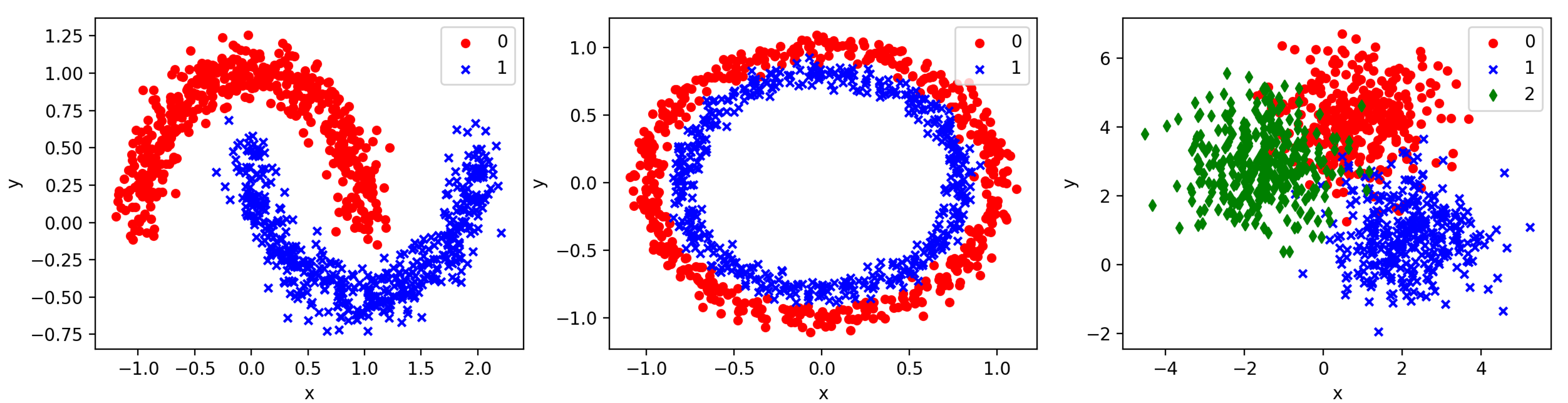
Figure 3: Three 2-dimensional datasets.

Text Classification:

For text classification we use the datasets Question Classification Li and Roth (2002), which contains short questions along with the type of answer expected, and Sentence Classification Chambers (2013), which consists of sentences selected from medical publications. Examples of instance/class pairs for the text classification datasets include ”Where is the Orinoco?” (class: ”location”) for the Question Classification dataset, and ”New types of potent force clamps are discovered.” (class: ”author’s own work”) for the Sentence Classification dataset.

For these datasets that do not include crowd annotations, we synthesise annotations by simulating different annotators as follows: 1) Narrow Expert: has expertise in a single domain (i.e. class). For the instances of this class, the annotator will always provide the correct label. For other classes, a correct label will be provided with a probability of 0.65; otherwise, a random label will be selected with uniform probability; 2) Broad Expert: has expertise in every domain and only makes mistakes with a probability of 0.05; 3) Random Annotator: selects labels at random; 4) Adversarial Annotator: deliberately provides incorrect labels with a probability of 0.8.

For each of the datasets, we generated annotations using one narrow expert per class, one broad expert, one random annotator and one adversarial annotator, for a total of $|T|+3$ annotators, where $|T|$ is the number of classes in the dataset.

In order to evaluate the generality of our model, we also apply it to another task in which we have 5 annotators with different overall reliabilities for the text classification tasks. They produce incorrect labels with probabilities 0.1, 0.3, 0.5, 0.7, 0.9 respectively.

Real-World Crowdsourcing Annotators

Recognising Textual Entailment:

Finally, we evaluate our model on a real-world dataset for the recognising textual entailment (RTE) task Snow et al. (2008). Given a text pair, the annotator decides whether the hypothesis sentence can be inferred from the text fragment. The dataset includes both ground truth and crowdsourced labels from 164 annotators.

Table 1 shows the number of instances of each class in the above-mentioned datasets.

Dataset	Class	# Instances
moon	0/1	500/500
circle	0/1	500/500
3-class	0/1/2	334/333/333
	DESCRIPTION (DESC)	1162
	ENTITY (ENTY)	1250
Question	ABBREV. (ABBR)	86
Classification	HUMAN (HUM)	1223
	NUMERIC (NUM)	896
	LOCATION (LOC)	835
	AIMX	94
Sentence	OWNX	427
Classification	CONT	104
	BASE	33
	MISC	852
RTE	0/1	400/400

Table 1: Classes and per-class instance counts.

4.2 Experimental and Model Settings

Datasets	Classifier	# Units
2-Dimensional Datasets (3 datasets)	2D$\rightarrow$FNN	5
Text Classification (2 datasets)	BoW$\rightarrow$FNN	100
	Avg. $\rightarrow$FNN	50
	Embed.$\rightarrow$LSTM$\rightarrow$FNN	100
RTE	Cat. Avg. $\rightarrow$FNN	100
	Embed.$\rightarrow$LSTM$\rightarrow$FNN Bowman et al. (2015)	200

Table 2: Classifiers used in the experiments.

Our model was implemented using the Chainer deep learning framework Tokui et al. (2015).

Classifier:

As shown in Table 2, in each experiment the output of the classifier is generated by a feed-forward neural network (FNN). Each FNN consists of an input layer, two hidden layers and a softmax output layer. The number of hidden units in each layer is listed in the third column of the table. The ReLU activation function Nair and Hinton (2010) was applied after each hidden layer. The output size of all the Long Short-Term Memory (LSTM; Hochreiter and Schmidhuber, 1997) layers in our experiments is 100.

For the 2-dimensional classification task, each instance is simply represented using its position in 2-dimensional space. For the text classification tasks, we investigated 3 methods of representing the sentences: bag-of-words (BoW) weighted by Term Frequency–Inverse Document Frequency (TFIDF), an average word embedding (Avg.) and the output at the last step of an LSTM layer (Embed.$\rightarrow$LSTM). For the embedding we use word2vec embeddings pre-trained on Google News Mikolov et al. (2013) for the question classification and RTE tasks, and a pre-trained embedding Pyysalo et al. (2013) trained on a combination of English Wikipedia, PubMed and PMC texts for the sentence classification task.

For the RTE task, we implemented two classifiers. For the first one, each instance (i.e. a sentence pair) was represented as a concatenation of the average word embedding for each sentence (Cat. Avg.). We also implemented  Bowman et al. Bowman et al. (2015), which runs each sentence through an LSTM, concatenates the outputs, and then feeds the concatenated output to an FNN with tanh activations.

Reliability Estimator:

We model the reliability estimator as an FNN. Its structure is the same as the classifier, albeit with different sizes of the two hidden layers. For the experiments listed in Table 2, the number of units of each hidden layer in the FNN are 5, 100, 25, 25, 50, and 100 respectively. The input to the estimator is the concatenation of the instance $\mathbf{x}_{i}$ (i.e. its original feature vector or the output of the last hidden layer of the classifier) and a one-hot vector representing the annotator identity.

Learning Settings:

For every experiment we use the Adam Kingma and Ba (2015) optimiser with a weight decay rate $0.001$, a gradient clipping of $5.0$, $\alpha=0.001$, $\beta_{1}=0.9$ and $\beta_{2}=0.999$. We pre-train the classifier and reliability estimator for 200 epochs, using both majority voting and the model proposed by Dawid and Skene Dawid and Skene (1979). The maximum number of outer iterations is set to 500 and 20 for EM training and cross entropy training respectively. The number of inner iterations is 50 in both cases.

True Label Prediction and Reliability Estimation:

After training, for each instance $\boldsymbol{\mathbf{x}}_{i}$ we take its underlying label to be the most probable label according to the posterior of $t_{i}$ (see Equation 4). We compared our predicted labels to the following state-of-the-art baselines: Majority Voting (MV), DS Dawid and Skene (1979), GLAD Whitehill et al. (2009), LFC Raykar et al. (2010), CUBAM Welinder et al. (2010),  Yan et al. Yan et al. (2010), KOS Karger et al. (2011), VI Liu et al. (2012), BCC Kim and Ghahramani (2012), MINIMAX Zhou et al. (2012), MACE Hovy et al. (2013), CATD Li et al. (2014a), PM Li et al. (2014b) and EM-MV and Opt Zhang et al. (2014).

Note that CUBAM, Yan et al. Yan et al. (2010), KOS and VI are only suitable for aggregating binary labels, and  Yan et al. Yan et al. (2010) is the state-of-the-art method that models per-instance reliability. We take the reliability of annotator $j$ on instance $\boldsymbol{\mathbf{x}}_{i}$ to be the posterior probability that $r_{ij}$ is 1 (see Equation 5).

5 Results and Analysis

We measure the inter-annotator agreement (IAA) of each dataset. Fleiss’s kappa Fleiss et al. (2013), denoted by $\kappa$, is measured for the 2-dimensional and text classification datasets, and Krippendorff’s alpha Krippendorff (1970) is calculated for the RTE dataset. We find that the IAA values indicate slight agreement among annotators for all datasets.

Our experiments using different settings are shown as follows: our model is denoted by O, with M and D denoting the model pre-trained using MV and DS respectively. E denotes training using expectation maximisation, while C denotes cross entropy training. AL and JT denote cross entropy training done alternatingly and jointly, respectively.

In the rest of this section, Tables 3, 4, 5, 6, 5 and 7 and Tables 8, 9 and 10 present the results on the synthetic datasets and RTE dataset respectively. For the synthetic datasets, in Tables 3, 4, 5, 6 and 5, we first consider a scenario where we have multiple narrow experts (N), one broad expert (B), one random annotator (R) and one adversarial annotator (A). In Table 7, we further consider a scenario with 5 annotators, each of differing reliability, as explained in Section 4.1.

Table 3 shows that our method performs well on the 2-dimensional datasets, obtaining higher label prediction F1 scores than the baselines. We omit the analysis of the true label prediction and reliability estimation results on these datasets as all models performed similarly, choosing instead to focus the discussion on the results for the NLP tasks.

	2-Dimensional Datasets
	moon	circle	3-class
	$\kappa=0.029$	$\kappa=0.029$	$\kappa=0.153$
MV	84.6	84.6	89.0
DS Dawid and Skene (1979)	97.8	97.9	99.4
GLAD Whitehill et al. (2009)	97.9	97.9	93.7
LFC Raykar et al. (2010)	97.9	97.9	99.4
CUBAM Welinder et al. (2010)	97.9	97.9	-
Yan et al. Yan et al. (2010)	84.1	84.1	-
KOS Karger et al. (2011)	96.7	96.7	-
VI Liu et al. (2012)	97.9	97.9	-
BCC Kim and Ghahramani (2012)	97.9	97.9	99.4
MINIMAX Zhou et al. (2012)	97.9	97.9	99.2
MACE Hovy et al. (2013)	97.8	97.9	97.0
CATD Li et al. (2014a)	94.5	94.5	94.3
PM Li et al. (2014b)	94.5	94.5	94.3
EM-MV Zhang et al. (2014)	97.9	97.9	96.3
EM-Opt Zhang et al. (2014)	72.7	72.7	93.2
O-ME	97.0	97.7	94.8
O-MC	97.3	98.9	99.3
O-DE	91.2	97.2	96.5
O-DC-AL	99.7	99.7	99.5
O-DC-JT	99.8	99.6	99.5

Table 3: F1 scores of predicted labels on the 2-dimensional datasets when using the output of the last hidden layer of the classifier to represent an instance for the reliability estimator.

5.1 Classifier and Reliability Estimator

In order to explore the separate performance contribution of classifier and reliability estimator, we compare the performance of our model to a classifier pre-trained using DS labels, as well as a variant of our model without the reliability estimator, i.e. setting all the annotators have the same reliability on all the instances.

As shown in Tables 4, 7 and 8, the pre-trained classifier performed worse than some aggregation methods. This indicates that the noise in the labels predicted by DS has an adverse effect on the training of the classifier. The much lower performance of the model with the reliability estimator removes hints at the importance of modelling per-annotator reliability to ensure accurate predictions.

5.2 Instance Representation for Reliability Estimator

For the representation of the instance $\mathbf{x}_{i}$ as it is fed to the reliability estimator, we compared the performance of using the original feature vector of $\mathbf{x}_{i}$ to using the last hidden layer output of the classifier (which we refer to as the “full model”).

We found that using the hidden layer representation can not only improve the label prediction performance (see Tables 4, 7 and 8), but also sped up the training compared to using the feature vector directly. The hidden layer representation allows us to reduce the number of parameters in the model, by sharing parameters with the classifier.

5.3 Full Model on Synthetic Datasets

Based on the results of the full model in Table 4, we can conclude that per-instance reliability modelling is beneficial to the label prediction task, and using the average pre-trained embedding can result in slightly better performance. It is worth noting that the method used to pre-train the model had a noticeable effect on its performance, with better F1 scores being obtained when using DS pre-training. In the following experiments we only consider models pre-trained using the DS algorithm.

	Question Classification		Sentence Classification
	$\kappa=0.094$		$\kappa=0.0634$
	BoW	Avg.	BoW	Avg.
MV	78.8	78.8	71.3	71.3
DS Dawid and Skene (1979)	98.3	98.3	97.3	97.3
GLAD Whitehill et al. (2009)	87.1	87.1	79.9	79.9
LFC Raykar et al. (2010)	98.2	98.2	97.0	97.0
BCC Kim and Ghahramani (2012)	98.3	98.3	98.1	98.1
MINIMAX Zhou et al. (2012)	28.2	28.2	50.9	50.9
MACE Hovy et al. (2013)	91.6	91.6	63.6	63.6
CATD Li et al. (2014a)	91.1	91.1	92.2	92.2
PM Li et al. (2014b)	91.1	91.1	92.2	92.2
EM-MV Zhang et al. (2014)	88.3	88.3	66.9	66.9
EM-Opt Zhang et al. (2014)	13.5	13.5	26.5	26.5
Classifier (pre-trained by DS labels)	92.3	86.5	89.6	85.4
O-DE (without reliability estimator)	92.1	91.2	77.6	87.1
O-DC-AL (without reliability estimator)	90.5	93.2	84.0	88.2
O-DC-JT (without reliability estimator)	88.7	91.1	78.5	87.4
O-DE (using feature vector)	95.1	97.0	88.9	97.8
O-DC-AL (using feature vector)	97.5	98.9	97.2	97.5
O-DC-JT (using feature vector)	97.5	98.9	97.2	97.5
O-ME (full model)	92.4	95.0	84.4	89.2
O-MC (full model)	97.2	98.3	90.6	94.6
O-DE (full model)	98.0	98.3	97.7	98.9
O-DC-AL (full model)	98.3	98.6	97.6	97.9
O-DC-JT (full model)	98.7	99.0	97.3	97.8

Table 4: F1 scores of predicted labels on the text classification datasets.

	Question Classification
	DESC	ENTY	ABBR	HUM	NUM	LOC	Accuracy
1 (N)	99	1	0	0	0	0	100
2 (N)	0	100	0	0	0	0	100
3 (N)	31	13	40	5	2	9	100
4 (N)	0	0	0	100	0	0	100
5 (N)	0	0	0	0	100	0	100
6 (N)	0	0	0	0	0	100	100
7 (B)	20	0	0	77	0	3	100
8 (R)	30	32	8	8	15	7	100
9 (A)	45	19	9	14	5	8	100

Table 5: Number of correctly labelled examples for each annotator (N: narrow expert, B: broad expert, R: random annotator and A: adversarial annotator) among the 100 instances with highest per-instance reliability on the question classification dataset.

	Question Classification
	DESC	ENTY	ABBR	HUM	NUM	LOC	Overall
1 (N)	90.6	24.4	35.5	21.4	26.6	22.2	36.8
2 (N)	28.7	92.3	26.6	25.2	24.3	26.7	37.3
3 (N)	24.7	24.9	75.8	23.5	24.7	23.6	32.9
4 (N)	27.5	26.3	32.3	93.4	24.2	23.7	37.9
5 (N)	25.6	21.9	25.2	25.7	93.8	26.0	36.4
6 (N)	26.4	25.0	24.1	22.1	27.5	94.4	36.6
7 (B)	94.3	93.5	95.1	94.2	93.4	93.9	94.2
8 (R)	5.60	6.30	8.40	4.80	6.20	5.90	6.20
9 (A)	9.10	8.90	12.0	8.20	7.90	8.30	9.10

Table 6: Average reliability of each annotator among the 100 instances with the highest per-instance reliability on the question classification dataset.

In order to investigate whether our method can successfully capture per-instance annotator reliability, for each annotator, we counted the number of correctly labelled instances and calculated the average reliability for each class among the top 100 instances with the highest per-instance reliability as shown in Table 5 and 6. The cells with grey background colour indicate which domain, or class, the annotator has expertise in. It can be seen that all annotators obtain high accuracy on these instances. In general our method also captured the varying expertise of each narrow annotator, estimating their reliability on instances belonging to the corresponding classes as particularly high.

For these experiments in Table 7, we also investigated the performance when using two different classification models. As seen in this table, both of them outperformed all baselines significantly.

	Question Classification		Sentence Classification
	$\kappa=0.126$		$\kappa=0.0776$
	FNN	LSTM+FNN	FNN	LSTM+FNN
MV	71.8	71.8	65.8	65.8
DS Dawid and Skene (1979)	90.1	90.1	83.9	83.9
GLAD Whitehill et al. (2009)	80.9	80.9	71.8	71.8
LFC Raykar et al. (2010)	88.3	88.3	80.3	80.3
BCC Kim and Ghahramani (2012)	90.4	90.4	85.6	85.6
MINIMAX Zhou et al. (2012)	30.4	30.4	44.0	44.0
MACE Hovy et al. (2013)	84.6	84.6	62.4	62.4
CATD Li et al. (2014a)	85.2	85.2	80.5	80.5
PM Li et al. (2014b)	85.2	85.2	80.5	80.5
EM-MV Zhang et al. (2014)	75.4	75.4	56.6	56.6
EM-Opt Zhang et al. (2014)	19.4	19.4	14.4	14.4
Classifier (pre-trained by DS labels)	89.7	76.6	79.6	78.7
O-DE (without reliability estimator)	91.9	91.0	80.1	82.5
O-DC-AL (without reliability estimator)	91.8	91.2	80.0	83.5
O-DC-JT (without reliability estimator)	91.5	91.6	79.3	83.5
O-DE (using feature vector)	94.3	-	81.7	-
O-DC-AL (using feature vector)	94.1	-	86.2	-
O-DC-JT (using feature vector)	94.1	-	86.2	-
O-DE (full model)	94.5	94.1	86.1	86.1
O-DC-AL (full model)	94.7	96.0	90.3	88.5
O-DC-JT (full model)	95.1	95.1	88.5	89.0

Table 7: F1 scores on text classification tasks when only the reliability differs between the annotators.

5.4 Full Model on RTE Dataset

Table 8 presents the label prediction performance on the RTE dataset. As not every annotator has provided labels for every instance in this dataset, for both the EM and cross entropy training we simply omitted missing instance/annotator pairs when calculating the loss functions. As seen in the table, most of the baselines obtained high performance as the textual entailment recognition task is easy for non-expert annotators. However, our full model still achieved better prediction performance than all of the baseline methods.

Method	F-measure
MV	91.9
DS Dawid and Skene (1979)	92.6
GLAD Whitehill et al. (2009)	92.4
LFC Raykar et al. (2010)	92.5
CUBAM Welinder et al. (2010)	92.6
Yan et al. Yan et al. (2010)	90.4
KOS Karger et al. (2011)	63.2
VI Liu et al. (2012)	92.5
BCC Kim and Ghahramani (2012)	92.3
MINIMAX Zhou et al. (2012)	92.4
MACE Hovy et al. (2013)	92.4
CATD Li et al. (2014a)	92.3
PM Li et al. (2014b)	92.0
EM-MV Zhang et al. (2014)	92.5
EM-Opt Zhang et al. (2014)	92.4
Classifier (pre-trained by DS labels)	89.9
O-DC-JT (FNN) (without reliability estimator)	90.2
O-DC-JT (FNN) (using feature vector)	92.6
O-DE (FNN) (full model)	92.9
O-DC-AL (FNN) (full model)	92.8
O-DC-JT (FNN) (full model)	93.0
O-DE (LSTM+FNN) (full model)	92.7
O-DC-AL (LSTM+FNN) (full model)	92.8
O-DC-JT (LSTM+FNN) (full model)	92.8

Table 8: Performance of predicted labels on the RTE dataset (Krippendorff’s alpha $=0.0995$).

We also investigated the effectiveness of our model for removing noisy labels. We compare our model to the five best-performing baselines (DS, LFC, CUBAM, VI and EM-MV in Table 8). Each of these models are trained on the RTE dataset, after which the least reliable annotation for each instance is removed. We use the per-instance reliability for our model, the global reliability score of each annotator for LFC, CUBAM and VI, and the per-category annotator reliability for DS and EM-MV as the measure of the reliability of each annotation. For each of these models, we then retrain the models in Table 8 using the denoised dataset; the difference in performance can be seen in Table 9. We can see that using per-instance reliability results in the largest improvement, while only considering the annotators’ overall reliability may cause a reduction in performance.

In order to analyse the per-instance reliability of the human annotators, for each annotator we rank the instances according to the annotator’s per-instance reliability. We look at the top 15 and bottom 15 instances, then count how many of them were correctly labelled (Cor. Labels) as well as the average reliability on these instances (Avg. Reliability). Table 10 shows the results of five annotators. It can be seen that each annotator has considerably different reliabilities across instances.

Method	LFC	CUBAM	VI	DS	EM-MV	Ours
MV	-0.2	-0.9	+0.6	-0.2	-0.2	+0.8
DS Dawid and Skene (1979)	0	-0.2	+0.1	0	0	+0.6
GLAD Whitehill et al. (2009)	+0.2	0	0	+0.2	-0.3	+0.2
LFC Raykar et al. (2010)	+0.1	-0.1	+0.3	+0.1	+0.1	+0.6
CUBAM Welinder et al. (2010)	+0.3	0	+0.4	+0.3	-0.2	+0.9
Yan et al. Yan et al. (2010)	+1.5	+0.4	+2.3	+1.5	+0.8	+2.5
KOS Karger et al. (2011)	+0.7	+3.9	+11.3	+0.7	+13.4	+17.3
VI Liu et al. (2012)	+0.1	+0.1	+0.1	+0.1	+0.2	+0.6
BCC Kim and Ghahramani (2012)	+0.3	+0.2	+0.3	+0.3	+0.4	+0.8
MINIMAX Zhou et al. (2012)	+0.3	-0.4	+0.7	+0.3	+0.2	+0.7
MACE Hovy et al. (2013)	+0.2	-0.2	0	+0.2	0	+0.4
CATD Li et al. (2014a)	+0.3	-0.8	-0.2	+0.3	+0.2	+0.3
PM Li et al. (2014b)	+0.9	0	+0.3	+0.9	+0.1	+0.9
EM-MV Zhang et al. (2014)	+0.7	+0.6	+0.7	+0.7	+0.7	+1.1
EM-Opt Zhang et al. (2014)	+0.2	+0.5	+0.2	+0.2	+0.6	+0.7
O-DC-JT (FNN) (full model)	+0.1	0	+0.3	+0.1	+0.1	+0.5

Table 9: F1 score improvements after removing the label produced by the least reliable annotator by using the estimated overall reliability (LFC, CUBAM, VI, DS, EM-MV) and per-instance reliability (Ours).

		True Entailment		False Entailment
	Annotator	#Cor. Labels	Avg. Reliability	#Cor. Labels	Avg. Reliability	Acc.
Top 15 Instances	1	15	95.5	-	-	100
	2	15	92.6	-	-	100
	3	10	88.4	3	86.9	86.7
	4	11	94.2	2	92.6	86.7
	5	8	71.9	2	23.7	66.7
Bottom 15 Instances	1	4	0.1	2	0.1	40
	2	1	1.0	8	51.4	60
	3	0	9.7	1	13.8	6.6
	4	2	28.6	5	63.1	46.7
	5	3	22.3	2	23.7	33.3

Table 10: Number of correct labels and average reliability for each annotator among the instances with highest and lowest per-instance reliability on the RTE dataset.

5.5 Training Stability

Pre-training:

As discussed in Section 3.2, the predicted labels produced by a simpler method are used for pre-training. Although these labels are not perfect, we assume that our method can still learn some useful information from them for a better starting point than random parameter initialisation.

EM and Cross Entropy Training:

From Tables 3, 4, 7 and 8, it can be seen that, in most cases, using cross entropy achieved much better and more stable performance than the models learned using EM training. We also noticed that the objective function would improve when using cross entropy training, and tended to converge faster in our experiments—generally within just a few epochs. Therefore, we recommend to use this training method in practice.

Early Stopping:

When using both EM and cross entropy training, we found that even if the objective function improved between iterations, the label prediction performance would eventually start to decrease. It is worth to investigate the reason for this phenomenon. To counteract this issue we used early stopping, where training is halted when the objective function does not improve more than 0.001 between iterations. Another option is to reduce the maximum number of outer iterations, e.g. to 20.

6 Conclusion and Future Work

We propose a novel probabilistic model which learns from noisy labels produced by multiple annotators for NLP crowdsourcing tasks by incorporating a classifier and a reliability estimator. Our work constitutes the first effort to model the per-instance reliability of annotators for both binary and multi-class NLP labelling tasks. We investigate two methods of training our model using the EM algorithm and cross entropy. Experimental results on 6 datasets including synthetic and real datasets demonstrate that our method can not only capture the per-instance reliability of each annotator, but also obtain better label prediction and the least reliable annotator detection performance compared to state-of-the-art baselines.

For future work, we plan to apply our model to other NLP tasks such as relation extraction and named entity recognition. We also plan to investigate the use of variational inference Jordan et al. (1999) as a means of training our model. Using variational inference might improve the stability and performance of our model.

References

- Aroyo and Welty (2013) Lora Aroyo and Chris Welty. 2013. Measuring crowd truth for medical relation extraction. In AAAI 2013 Fall Symposium on Semantics for Big Data, pages 1–9, Arlington, Virginia.
- Bonald and Combes (2017) Thomas Bonald and Richard Combes. 2017. A minimax optimal algorithm for crowdsourcing. In Advances in Neural Information Processing Systems 30 (NIPS), pages 4352–4360. Curran Associates, Inc.
- Bowman et al. (2015) Samuel R. Bowman, Gabor Angeli, Christopher Potts, and Christopher D. Manning. 2015. A large annotated corpus for learning natural language inference. In Proceedings of the 2015 Conference on Empirical Methods in Natural Language Processing (EMNLP), pages 632–642, Lisbon, Portugal. Association for Computational Linguistics.
- Chambers (2013) America Chambers. 2013. Statistical Models for Text Classification and Clustering: Applications and Analysis. Ph.D. thesis, University of California, Irvine.
- Cortes and Vapnik (1995) Corinna Cortes and Vladimir Vapnik. 1995. Support-vector networks. Machine Learning, 20(3):273–297.
- Dawid and Skene (1979) Alexander Philip Dawid and Allan M Skene. 1979. Maximum likelihood estimation of observer error-rates using the em algorithm. Applied statistics, pages 20–28.
- Demartini et al. (2012) Gianluca Demartini, Djellel Eddine Difallah, and Philippe Cudré-Mauroux. 2012. ZenCrowd: leveraging probabilistic reasoning and crowdsourcing techniques for large-scale entity linking. In Proceedings of the 21st international conference on World Wide Web (WWW), WWW ’12, pages 469–478, New York, NY, USA. Association for Computing Machinery.
- Dempster et al. (1977) Arthur P. Dempster, Nan Laird, and Donald B. Rubin. 1977. Maximum likelihood from incomplete data via the EM algorithm. Journal of the Royal Statistical Society, B39:1–38.
- Donmez and Carbonell (2008) Pinar Donmez and Jaime G. Carbonell. 2008. Proactive learning: cost-sensitive active learning with multiple imperfect oracles. In Proceedings of the 17th ACM Conference on Information and Knowledge Management (CIKM), CIKM ’08, pages 619–628, New York, NY, USA. Association for Computing Machinery.
- Fleiss et al. (2013) Joseph L Fleiss, Bruce Levin, and Myunghee Cho Paik. 2013. Statistical methods for rates and proportions, 3 edition. John Wiley & Sons.
- Gurevych and Kim (2013) Iryna Gurevych and Jungi Kim, editors. 2013. The People’s Web Meets NLP: Collaboratively Constructed Language Resources. Springer-Verlag Berlin Heidelberg.
- Hochreiter and Schmidhuber (1997) Sepp Hochreiter and Jürgen Schmidhuber. 1997. Long Short-Term Memory. Neural Computation, 9(8):1735–1780.
- Hovy et al. (2013) Dirk Hovy, Taylor Berg-Kirkpatrick, Ashish Vaswani, and Eduard Hovy. 2013. Learning whom to trust with MACE. In Proceedings of the 2013 Conference of the North American Chapter of the Association for Computational Linguistics: Human Language Technologies (NAACL-HLT), pages 1120–1130, Atlanta, Georgia. Association for Computational Linguistics.
- Jordan et al. (1999) Michael I. Jordan, Zoubin Ghahramani, Tommi S. Jaakkola, and Lawrence K. Saul. 1999. An introduction to variational methods for graphical models. Machine Learning, 37(2):183–233.
- Karger et al. (2011) David R. Karger, Sewoong Oh, and Devavrat Shah. 2011. Iterative learning for reliable crowdsourcing systems. In J. Shawe-Taylor, R. S. Zemel, P. L. Bartlett, F. Pereira, and K. Q. Weinberger, editors, Advances in Neural Information Processing Systems 24 (NIPS), pages 1953–1961. Curran Associates, Inc.
- Kim and Ghahramani (2012) Hyun-Chul Kim and Zoubin Ghahramani. 2012. Bayesian classifier combination. In Proceedings of the Fifteenth International Conference on Artificial Intelligence and Statistics, volume 22 of Proceedings of Machine Learning Research, pages 619–627, La Palma, Canary Islands. PMLR.
- Kingma and Ba (2015) Diederik P Kingma and Jimmy Ba. 2015. Adam: A method for stochastic optimization. In Proceedings of the International Conference on Learning Representations (ICLR), pages 1–13, San Diego, CA, USA.
- Krippendorff (1970) Klaus Krippendorff. 1970. Estimating the reliability, systematic error and random error of interval data. Educational and Psychological Measurement, 30(1):61–70.
- Li et al. (2017) Maolin Li, Nhung Nguyen, and Sophia Ananiadou. 2017. Proactive learning for named entity recognition. In BioNLP 2017, pages 117–125, Vancouver, Canada. Association for Computational Linguistics.
- Li et al. (2014a) Qi Li, Yaliang Li, Jing Gao, Lu Su, Bo Zhao, Murat Demirbas, Wei Fan, and Jiawei Han. 2014a. A confidence-aware approach for truth discovery on long-tail data. Proceedings of the VLDB Endowment, 8(4):425–436.
- Li et al. (2014b) Qi Li, Yaliang Li, Jing Gao, Bo Zhao, Wei Fan, and Jiawei Han. 2014b. Resolving conflicts in heterogeneous data by truth discovery and source reliability estimation. In Proceedings of the 2014 ACM SIGMOD International Conference on Management of Data, SIGMOD ’14, pages 1187–1198, New York, NY, USA. Association for Computing Machinery.
- Li and Roth (2002) Xin Li and Dan Roth. 2002. Learning question classifiers. In Proceedings of the 19th International Conference on Computational Linguistics (COLING), volume 1, pages 1–7, Taipei, Taiwan. Association for Computational Linguistics.
- Liu et al. (2012) Qiang Liu, Jian Peng, and Alexander T Ihler. 2012. Variational inference for crowdsourcing. In F. Pereira, C. J. C. Burges, L. Bottou, and K. Q. Weinberger, editors, Advances in Neural Information Processing Systems 25 (NIPS), pages 692–700. Curran Associates, Inc.
- Mikolov et al. (2013) Tomas Mikolov, Ilya Sutskever, Kai Chen, Greg S Corrado, and Jeff Dean. 2013. Distributed representations of words and phrases and their compositionality. In Advances in neural information processing systems 26 (NIPS), pages 3111–3119. Curran Associates, Inc.
- Nair and Hinton (2010) Vinod Nair and Geoffrey E Hinton. 2010. Rectified linear units improve restricted boltzmann machines. In Proceedings of the 27th international conference on machine learning (ICML-10), pages 807–814.
- Nguyen et al. (2017) An Thanh Nguyen, Byron Wallace, Junyi Jessy Li, Ani Nenkova, and Matthew Lease. 2017. Aggregating and predicting sequence labels from crowd annotations. In Proceedings of the 55th Annual Meeting of the Association for Computational Linguistics (Volume 1: Long Papers) (ACL), pages 299–309, Vancouver, Canada. Association for Computational Linguistics.
- Poesio et al. (2017) Massimo Poesio, Jon Chamberlain, and Udo Kruschwitz. 2017. Crowdsourcing. In Nancy Ide and James Pustejovsky, editors, Handbook of Linguistic Annotation, pages 277–295. Springer Netherlands, Dordrecht.
- Poesio et al. (2013) Massimo Poesio, Jon Chamberlain, Udo Kruschwitz, Livio Robaldo, and Luca Ducceschi. 2013. Phrase detectives: Utilizing collective intelligence for internet-scale language resource creation. ACM Transactions on Interactive Intelligent Systems (TiiS), 3(1):3:1–3:44.
- Pyysalo et al. (2013) Sampo Pyysalo, Filip Ginter, Hans Moen, Tapio Salakoski, and Sophia Ananiadou. 2013. Distributional semantics resources for biomedical text processing. In Proceedings of the Fifth International Symposium on Languages in Biology and Medicine (LBM), pages 39–44, Tokyo, Japan.
- Raykar et al. (2010) Vikas C. Raykar, Shipeng Yu, Linda H. Zhao, Gerardo Hermosillo Valadez, Charles Florin, Luca Bogoni, and Linda Moy. 2010. Learning from crowds. The Journal of Machine Learning Research, 11(Apr):1297–1322.
- Rodrigues et al. (2014) Filipe Rodrigues, Francisco Pereira, and Bernardete Ribeiro. 2014. Sequence labeling with multiple annotators. Machine Learning, 95(2):165–181.
- Sheshadri and Lease (2013) Aashish Sheshadri and Matthew Lease. 2013. SQUARE: a benchmark for research on computing crowd consensus. In Proceedings of the 1st AAAI Conference on Human Computation (HCOMP), pages 156–164, Palm Springs, CA, USA. The AAAI Press.
- Snow et al. (2008) Rion Snow, Brendan O’Connor, Daniel Jurafsky, and Andrew Ng. 2008. Cheap and fast – but is it good? evaluating non-expert annotations for natural language tasks. In Proceedings of the 2008 Conference on Empirical Methods in Natural Language Processing (EMNLP), pages 254–263, Honolulu, Hawaii. Association for Computational Linguistics.
- Tokui et al. (2015) Seiya Tokui, Kenta Oono, Shohei Hido, and Justin Clayton. 2015. Chainer: a next-generation open source framework for deep learning. In Proceedings of Workshop on Machine Learning Systems (LearningSys) in The Twenty-ninth Annual Conference on Neural Information Processing Systems (NIPS), pages 1–6.
- Wang and Bi (2017) Xin Wang and Jinbo Bi. 2017. Bi-convex optimization to learn classifiers from multiple biomedical annotations. IEEE/ACM Transactions on Computational Biology and Bioinformatics, 14(3):564–575.
- Welinder et al. (2010) Peter Welinder, Steve Branson, Pietro Perona, and Serge J Belongie. 2010. The multidimensional wisdom of crowds. In Advances in Neural Information Processing Systems 23 (NIPS), pages 2424–2432. Curran Associates, Inc.
- Whitehill et al. (2009) Jacob Whitehill, Ting-fan Wu, Jacob Bergsma, Javier R. Movellan, and Paul L. Ruvolo. 2009. Whose vote should count more: Optimal integration of labels from labelers of unknown expertise. In Advances in Neural Information Processing Systems 22 (NIPS), pages 2035–2043. Curran Associates, Inc.
- Yan et al. (2010) Yan Yan, Romer Rosales, Glenn Fung, Mark Schmidt, Gerardo Hermosillo, Luca Bogoni, Linda Moy, and Jennifer Dy. 2010. Modeling annotator expertise: Learning when everybody knows a bit of something. In Proceedings of the Thirteenth International Conference on Artificial Intelligence and Statistics, volume 9 of Proceedings of Machine Learning Research, pages 932–939, Chia Laguna Resort, Sardinia, Italy. PMLR.
- Yan et al. (2014) Yan Yan, Rómer Rosales, Glenn Fung, Ramanathan Subramanian, and Jennifer Dy. 2014. Learning from multiple annotators with varying expertise. Machine Learning, 95(3):291–327.
- Zhang et al. (2014) Yuchen Zhang, Xi Chen, Denny Zhou, and Michael I Jordan. 2014. Spectral methods meet EM: A provably optimal algorithm for crowdsourcing. In Advances in Neural Information Processing Systems 27 (NIPS), pages 1260–1268. Curran Associates, Inc.
- Zhou et al. (2012) Denny Zhou, Sumit Basu, Yi Mao, and John C. Platt. 2012. Learning from the wisdom of crowds by minimax entropy. In F. Pereira, C. J. C. Burges, L. Bottou, and K. Q. Weinberger, editors, Advances in Neural Information Processing Systems 25 (NIPS), pages 2195–2203. Curran Associates, Inc.