High-temperature analysis of the transverse dynamical two-point correlation function of the XX quantum-spin chain

Frank Göhmann, Karol K. Kozlowski and Junji Suzuki
Fakultät für Mathematik und Naturwissenschaften,

Bergische Universität Wuppertal, 42097 Wuppertal, Germany

Univ Lyon, ENS de Lyon, Univ Claude Bernard,

CNRS, Laboratoire de Physique, F-69342 Lyon, France

Department of Physics, Faculty of Science, Shizuoka University,

Ohya 836, Suruga, Shizuoka, Japan

Abstract

  • We analyse the transverse dynamical two-point correlation function of the XX chain by means of a thermal form factor series. The series is rewritten in terms of the resolvent and the Fredholm determinant of an integrable integral operator. This connects it with a matrix Riemann-Hilbert problem. We express the correlation function in terms of the solution of the matrix Riemann-Hilbert problem. The matrix Riemann-Hilbert problem is then solved asymptotically in the high-temperature limit. This allows us to obtain the leading high-temperature contribution to the two-point correlation function at any fixed space-time separation.

1 Introduction

In our recent work [13] we have developed an approach to the calculation of dynamical correlation functions of Yang-Baxter integrable lattice systems in equilibrium with a heat bath of temperature $T$. The basic idea was to combine a certain lattice realisation of a path integral for finite temperature dynamical correlation functions [27] with a thermal form factor expansion introduced in [10]. As a result we obtained a thermal form factor series for the dynamical two-point correlation functions in this class of systems.

A basic example, for which we worked out the series explicitly, is the transverse correlation function of the XX chain. The XX chain is a spin-$\frac{1}{2}$ model with Hamiltonian

$$H_{L}=J\sum_{j=1}^{L}\bigl{(}\sigma_{j-1}^{x}\sigma_{j}^{x}+\sigma_{j-1}^{y}\sigma_{j}^{y}\bigr{)}-\frac{h}{2}\sum_{j=1}^{L}\sigma_{j}^{z}\,.$$ (1)

Here the $\sigma_{j}^{\alpha}$, $\alpha=x,y,z$, are Pauli matrices acting on site $j\in\{1,\dots,L\}$ of an $L$-site lattice, and periodic boundary conditions, $\sigma_{0}^{\alpha}=\sigma_{L}^{\alpha}$, are implied. The parameters $J>0$ and $h>0$ are the strengths of the exchange interaction and of the external magnetic field.

The XX quantum-spin chain is particularly simple as an integrable model in that the derivative of the bare scattering phase in its Bethe Ansatz solution vanishes identically. It is also special since it maps to a model of non-interacting Fermions by means of a Jordan-Wigner transformation [22]. For these reasons rather much, in comparison with more generic integrable models, is known about its correlation functions. The longitudinal dynamical two-point function at finite temperature was calculated by Niemeijer [25] using the mapping to Fermions. We reproduced his result in a neat form from our thermal form factor series [13]. The transverse two-point function, defined as

$$\bigl{\langle}\sigma_{1}^{-}\sigma_{m+1}^{+}(t)\bigr{\rangle}_{T}=\lim_{L\rightarrow+\infty}\frac{\operatorname{tr}\{{\rm e}^{-H_{L}/T}\sigma_{1}^{-}{\rm e}^{{\rm i}H_{L}t}\sigma_{m+1}^{+}{\rm e}^{-{\rm i}H_{L}t}\}}{\operatorname{tr}\{{\rm e}^{-H_{L}/T}\}}\,,$$ (2)

where $t$ is the time variable and $\sigma^{\pm}=\frac{1}{2}(\sigma^{x}\pm{\rm i}\sigma^{y})$, is also well studied, but is much harder to access within the free Fermion approach. In fact, the finite-temperature analysis of (2) based on a Jordan-Wigner transformation stayed limited to the high-temperature asymptotics at short distances. Brandt and Jacoby [4] proved the rather well-known formula

$$\lim_{T\rightarrow+\infty}\bigl{\langle}\sigma_{1}^{-}\sigma_{1}^{+}(t)\bigr{\rangle}_{T}=\frac{1}{2}{\rm e}^{-{\rm i}ht-4J^{2}t^{2}}$$ (3)

for the auto-correlation function at infinite temperature. This was confirmed by Capel and Perk using a different method [6]. The same authors then obtained the first few terms in the high-temperature expansion of the auto-correlation function and of the nearest and next-to-nearest neighbour correlation functions at $h=0$ [26].

Deeper insight into the asymptotic behaviour of the transverse correlation function resulted from the study of different Fredholm determinant representations. The special case of vanishing magnetic field, $h=0$ in (1), maps to the critical transverse-field Ising chain [24], for which a Fredholm determinant representation of the auto-correlation function was obtained in [23]. Based on this Fredholm determinant representation the leading long-time asymptotic behaviour of the transverse auto-correlation function at finite temperature was computed in [9]. A Bethe Ansatz analysis of (2) was initiated by Colomo et al. in [7], where a Fredholm determinant representation of the correlation function at finite magnetic field was derived. This Fredholm determinant representation was then used for a long-time, large-distance asymptotic analysis of the correlation function at fixed temperature by Its et al. [17], who obtained the leading exponential term and the next-to-leading algebraic corrections. However, the constant term in the long-time, large-distance asymptotics in the critical regime $0\leq h<4J$ has never been calculated.

With our novel form factor series representation [13] we have the opportunity to revisit the problem of an efficient calculation of the transverse dynamical two-point function (2). The series is based on form factors of the quantum transfer matrix. It differs from the series employed by Its et al. in the derivation of their Fredholm determinant representation [17] of the correlation function. It gives us direct access [15] to the constant factor in the long-time, large-distance asymptotics of the correlation function in the so-called spacelike regime, where the spatial separation of two space-time points in appropriate units is larger than the time separation. In fact, the first term in the series determines the asymptotics in the spacelike regime. As such the series exhibits a striking similarity with the Borodin-Okounkov, Geronimo-Case formula [3, 12, 1] for a Toeplitz determinant generated by a symbol satisfying the hypotheses of the Szegö theorem.

For further asymptotic analysis we shall identify our series as being proportional to the Fredholm determinant of an integral operator of integrable type. In separate work [14] we shall show that this Fredholm determinant representation is highly efficient for the actual numerical calculation of the correlation function (2) in the critical as well as in the massive regime for generic values of distance, time and temperature.

In this work we will derive a matrix Riemann-Hilbert problem associated with our Fredholm determinant representation and express the two-point function (2) explicitly in terms of its solution. This matrix Riemann-Hilbert problem can be used to calculate the long-time, large-distance asymptotics of the correlation function in the timelike regime. As we shall see below, it can also be used to derive the high-temperature asymptotics of the two-point function for any fixed spatio-temporal separation. This is the main purpose of this work. We shall obtain a generalization of the Brandt-Jacoby formula (3) to any spatial separation of points. The generalization, stated more precisely in Theorem 3 below, is of the form

$$\bigl{\langle}\sigma_{1}^{-}\sigma_{m+1}^{+}(t)\bigr{\rangle}_{T}=\frac{1}{2}\biggl{(}-\frac{J}{T}\biggr{)}^{m}\exp\bigg{\{}{\rm i}c\tau-\frac{\tau^{2}}{4}+\int_{0}^{\tau}{\rm d}\tau^{\prime}\>u_{m}(\tau^{\prime})\biggr{\}}\\[4.30554pt] \times\frac{Q_{m+1}(-{\rm i})P_{m}^{\prime}(-{\rm i})-P_{m}(-{\rm i})Q_{m+1}^{\prime}(-{\rm i})}{\bigl{(}Q_{m+1}(-{\rm i})P_{m}^{\prime}(-{\rm i})-P_{m}(-{\rm i})Q_{m+1}^{\prime}(-{\rm i})\bigr{)}\bigr{|}_{\tau=0}}\bigl{(}1+{\cal O}(T^{-2})\bigr{)}\,.$$ (4)

Here $\tau=-4J\bigl{(}t-\frac{{\rm i}}{2T}\bigr{)}$, $c=\frac{h}{4J}$, and $P_{m}$ and $Q_{m+1}$ are polynomials whose coefficients depend on $\tau$. These coefficients are explicit but complicated rational combinations of modified Bessel functions. The same is true for the function $u_{m}$.

The paper is organized as follows. In Section 2 we recall and slightly rewrite the thermal form-factor series obtained in [13]. In Section 3 we recast the series in the form of a Fredholm-determinant representation. In Section 4 we work out the ‘integrable structure’ of the corresponding integral operator. Having in mind possible extensions to the more general XXZ chain we use a parameterization in terms of rapidity variables, entering the expression for the integration kernel through hyperbolic functions. In order to be self-contained we work out some of the basic features of the associated matrix Riemann-Hilbert problem in Section 5. In Section 6 we express the transverse correlation function in terms of the solution of the matrix Riemann-Hilbert problem. In Section 7 we transform the matrix Riemann-Hilbert problem to a certain standard form which, in Section 8, is asymptotically analysed in the high-temperature limit. Section 9 is devoted to the derivation of our main result, the high-temperature asymptotic formula (4). A short summary and conclusions are presented in Section 10. The appendices are devoted to the solution of the model Riemann-Hilbert problem appearing in the high-temperature asymptotic analysis, to working out some of the properties of the polynomials $P_{m}$ and $Q_{m+1}$ arising from this analysis, and to the presentation of examples of explicit high-temperature asymptotic formulae for small $m$.

2 Thermal form factor series

We start our analysis by recalling and slightly rewriting the thermal form factor series for the two-point function (2). For this purpose we have to introduce a number of basic functions.

2.1 One-particle energy and momentum

First of all we define the one-particle energy and momentum functions. The one-particle momentum as a function of the rapidity variable is defined by

$$p(\lambda)=-{\rm i}\ln\bigl{(}-{\rm i}\operatorname{th}(\lambda)\bigr{)}\,.$$ (5)

Here we may interpret the logarithm as its principal branch, meaning that we provide cuts in the complex plane from $-{\rm i}\pi/2$ to zero modulo ${\rm i}\pi$. Below we shall often encounter the derivative of the momentum function, most conveniently expressed as

$${\rm i}p^{\prime}(\lambda)=\frac{2}{\operatorname{sh}(2\lambda)}\,.$$ (6)

With this the one-particle energy can be defined as

$$\epsilon(\lambda)=h+2Jp^{\prime}(\lambda)\,,$$ (7)

where $h$ is the magnetic field and $J>0$ the exchange energy. In the following we restrict ourselves to the critical parameter regime

$$0<h<4J\,.$$ (8)

Because of the $\pi{\rm i}$-periodicity of the momentum, which is shared by all other functions in our form factor series, we may restrict ourselves to the ‘fundamental strip’

$${\cal S}=\Bigl{\{}\lambda\in{\mathbb{C}}\Big{|}-\frac{\pi}{4}\leq{\rm Im\,}\lambda<\frac{3\pi}{4}\Bigr{\}}$$ (9)

or rather think of the functions as being defined on a cylinder of circumference $\pi$.

It is easy to see that $\epsilon$ has precisely two roots

$$\lambda_{F}^{\pm}=\frac{{\rm i}\pi}{4}\pm z_{F}\,,\quad z_{F}=\frac{1}{2}\operatorname{arch}\biggl{(}\frac{4J}{h}\biggr{)}$$ (10)

in ${\cal S}$. These roots are called the Fermi rapidities. The value

$$p_{F}=p(\lambda_{F}^{-})=\arccos\biggl{(}\frac{h}{4J}\biggr{)}$$ (11)

of the momentum at the left Fermi rapidity will be called the Fermi momentum. Using the Fermi rapidities we may rewrite the one-particle energy as

$$\epsilon(\lambda)=-h\,p^{\prime}(\lambda)\operatorname{sh}(\lambda-\lambda_{F}^{-})\operatorname{sh}(\lambda-\lambda_{F}^{+})\,.$$ (12)

The functions $\epsilon$ and $p$ are real on the lines $x\pm{\rm i}\pi/4$, $x\in{\mathbb{R}}$, where they take the values

$\displaystyle\epsilon(x\pm{\rm i}\pi/4)=h\mp\frac{4J}{\operatorname{ch}(2x)}\,,$ (13a)
$\displaystyle p(x+{\rm i}\pi/4)=-\frac{\pi}{2}+2\operatorname{arctg}\bigl{(}{\rm e}^{-2x}\bigr{)}\,,$ (13b)
$\displaystyle p(x-{\rm i}\pi/4)=-\pi\operatorname{sign}(x)+\frac{\pi}{2}-2\operatorname{arctg}\bigl{(}{\rm e}^{-2x}\bigr{)}\,.$ (13c)

2.2 More functions appearing in the form factor series

In order to define the general term in the form factor series we have to introduce a few more functions. The one-particle energy determines the function

$$z(\lambda)=\frac{1}{2\pi{\rm i}}\ln\biggl{[}\operatorname{cth}\biggl{(}\frac{\epsilon(\lambda)}{2T}\biggr{)}\biggr{]}\,.$$ (14)

Another function needed below is the square of a generalized Cauchy determinant,

$${\cal D}\bigl{(}\{x_{j}\}_{j=1}^{m},\{y_{k}\}_{k=1}^{n}\bigr{)}=\frac{\bigl{[}\prod_{1\leq j<k\leq m}\operatorname{sh}^{2}(x_{j}-x_{k})\bigr{]}\bigl{[}\prod_{1\leq j<k\leq n}\operatorname{sh}^{2}(y_{j}-y_{k})\bigr{]}}{\prod_{j=1}^{m}\prod_{k=1}^{n}\operatorname{sh}^{2}(x_{j}-y_{k})}\,.$$ (15)
Refer to caption
Figure 1: Sketch of the hole and particle contours ${\cal C}_{h}$ and ${\cal C}_{p}$. The Fermi rapidity $\lambda_{F}^{-}$ is located inside ${\cal C}_{h}$, while $\lambda_{F}^{+}$ lies inside ${\cal C}_{p}$.

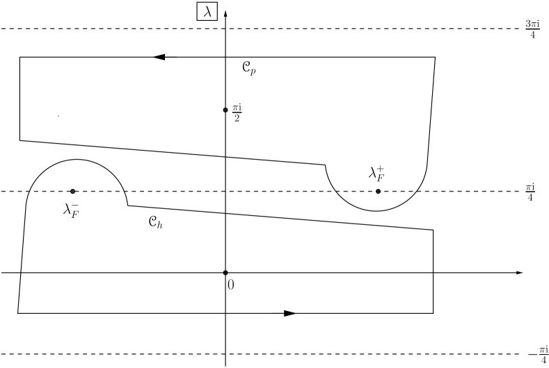
Two more functions that will play an important role in our analysis are defined as periodic Cauchy transforms with respect to a ‘hole contour’ ${\cal C}_{h}$ and a ‘particle contour’ ${\cal C}_{p}$ sketched in figure 1. The same simple, positively oriented contours will occur in the definition of the form factor series. They are defined in such a way that ${\cal C}_{h}$ encloses all roots of ${\rm e}^{-\epsilon(x)/T}-1$ inside the strip $-\pi/4<{\rm Im\,}x<\pi/4$ as well as the left Fermi rapidity $\lambda_{F}^{-}$, but no other roots of ${\rm e}^{-\epsilon(x)/T}-1$, while ${\cal C}_{p}$ encloses the roots of ${\rm e}^{-\epsilon(x)/T}-1$ inside the strip $\pi/4<{\rm Im\,}x<3\pi/4$ as well as the right Fermi rapidity $\lambda_{F}^{+}$ and again no other roots of ${\rm e}^{-\epsilon(x)/T}-1$.

Given these contours we define

$$\Phi_{h}(x)=\frac{{\rm i}p^{\prime}(x)}{2}\exp\biggl{\{}{\rm i}\int_{{\cal C}_{h}}{\rm d}\lambda\>p^{\prime}(\lambda)z(\lambda)\frac{\operatorname{sh}(x+\lambda)}{\operatorname{sh}(x-\lambda)}\biggr{\}}$$ (16)

for all $x\in{\cal S}\setminus{\cal C}_{h}$, and

$$\Phi_{p}(x)=\frac{{\rm i}p^{\prime}(x)}{2}\exp\biggl{\{}-{\rm i}\int_{{\cal C}_{p}}{\rm d}\lambda\>p^{\prime}(\lambda)z(\lambda)\frac{\operatorname{sh}(x+\lambda)}{\operatorname{sh}(x-\lambda)}\biggr{\}}$$ (17)

for all $x\in{\cal S}\setminus{\cal C}_{p}$. Being Cauchy transforms the functions $\Phi_{h}$ and $\Phi_{p}$ have jump discontinuities across the contours ${\cal C}_{h}$ and ${\cal C}_{p}$, respectively. Hence, each of these functions determines two functions on the respective contour by its boundary values from inside and outside the contour. We denote these functions by $\Phi_{h\pm}$ and $\Phi_{p\pm}$, where the plus sign stands for the boundary value from the left and the minus sign for the boundary value from the right of an oriented contour.

Fix $x\in\operatorname{Int}({\cal C}_{h})\cup\operatorname{Int}({\cal C}_{p})$. Then $\operatorname{sh}(x+\lambda)/\operatorname{sh}(x-\lambda)$ is a holomorphic function of $\lambda$ for all $\lambda\in{\cal S}\setminus\bigl{(}\operatorname{Int}({\cal C}_{h})\cup\operatorname{Int}({\cal C}_{p})\bigr{)}$. Since the integrands in (16), (17) are rapidly decaying for $\lambda\rightarrow\pm\infty$, we may deform the contours and conclude that

$\displaystyle\Phi_{h}(x)$ $\displaystyle=\Phi_{p}(x)$ for all $x\in\operatorname{Int}({\cal C}_{h})\cup\operatorname{Int}({\cal C}_{p}$), (18a)
$\displaystyle\Phi_{h+}(x)$ $\displaystyle=\Phi_{p}(x)$ for all $x\in{\cal C}_{h}$, (18b)
$\displaystyle\Phi_{p+}(x)$ $\displaystyle=\Phi_{h}(x)$ for all $x\in{\cal C}_{p}$. (18c)

2.3 The series

We can now recall the form factor series derived in [13]. Using the notation introduced above and performing some rather obvious simplifications it can be written as

$$\bigl{\langle}\sigma_{1}^{-}\sigma_{m+1}^{+}(t)\bigr{\rangle}_{T}=(-1)^{m}{\cal F}(m)\sum_{n=1}^{\infty}\frac{(-1)^{n}}{n!(n-1)!}\prod_{j=1}^{n}\int_{{\cal C}_{h}}\frac{{\rm d}x_{j}}{\pi{\rm i}}\frac{\Phi_{p}(x_{j}){\rm e}^{{\rm i}(mp(x_{j})-t\epsilon(x_{j}))}}{1-{\rm e}^{\epsilon(x_{j})/T}}\\ \times\prod_{k=1}^{n-1}\int_{{\cal C}_{p}}\frac{{\rm d}y_{k}}{\pi{\rm i}}\frac{{\rm e}^{-{\rm i}(mp(y_{k})-t\epsilon(y_{k}))}}{\Phi_{h}(y_{k})\bigl{(}1-{\rm e}^{-\epsilon(y_{k})/T}\bigr{)}}\>{\cal D}\bigl{(}\{x_{j}\}_{j=1}^{n},\{y_{k}\}_{k=1}^{n-1}\bigr{)}\,,$$ (19)

where

$${\cal F}(m)=\exp\biggl{\{}-\int_{{\cal C}_{h}^{\prime}\subset{\cal C}_{h}}{\rm d}\lambda\>z(\lambda)\int_{{\cal C}_{h}}{\rm d}\mu\>\operatorname{cth}^{\prime}(\lambda-\mu)z(\mu)\\ -{\rm i}mp_{F}-m\int_{{\cal C}_{h}}\frac{{\rm d}\lambda}{2\pi}p^{\prime}(\lambda)\ln\biggl{|}\operatorname{cth}\biggl{(}\frac{\epsilon(\lambda)}{2T}\biggr{)}\biggr{|}\biggr{\}}\,.$$ (20)

The contour ${\cal C}_{h}^{\prime}$ is tightly enclosed by ${\cal C}_{h}$.

3 Fredholm determinant representation

For the purpose of this work the series on the right hand side of (19) defines the correlation function. The task is to evaluate it numerically or asymptotically. An important step towards its efficient evaluation will be to rewrite the series as a Fredholm series, using a technique developed by Korepin and Slavnov in [20]. This is possible due to the occurrence of the square of the generalized Cauchy determinant on the right hand side of (19). Let

$$g(x)={\rm i}(mp(x)-t\epsilon(x))$$ (21)

and

$$w(x)=\frac{1}{\pi{\rm i}\Phi_{h}(x)\bigl{(}1-{\rm e}^{-\epsilon(x)/T}\bigr{)}}\,,\quad\overline{w}(x)=-\frac{\Phi_{p}(x)}{\pi{\rm i}\bigl{(}1-{\rm e}^{\epsilon(x)/T}\bigr{)}}\,.$$ (22)

Then

$$\bigl{\langle}\sigma_{1}^{-}\sigma_{m+1}^{+}(t)\bigr{\rangle}_{T}=(-1)^{m}{\cal F}(m)\sum_{n=1}^{\infty}\frac{1}{n!(n-1)!}\prod_{j=1}^{n}\int_{{\cal C}_{h}}{\rm d}x_{j}\>\overline{w}(x_{j}){\rm e}^{g(x_{j})}\\ \times\prod_{k=1}^{n-1}\int_{{\cal C}_{p}}{\rm d}y_{k}\>w(y_{k}){\rm e}^{-g(y_{k})}\>{\cal D}\bigl{(}\{x_{j}\}_{j=1}^{n},\{y_{k}\}_{k=1}^{n-1}\bigr{)}\,.$$ (23)

For the summation we note that ${\cal D}=C^{2}$, where

$$C=\lim_{{\rm Re\,}y_{n}\rightarrow+\infty}\frac{1}{2}\det_{n}\bigr{(}\varphi(x_{j},y_{k})\bigl{)}\,,\quad\varphi(x,y)=\frac{{\rm e}^{y-x}}{\operatorname{sh}(y-x)}\,.$$ (24)

It follows that

$\displaystyle\frac{1}{n!}\prod_{j=1}^{n}\int_{{\cal C}_{h}}{\rm d}x_{j}\>\overline{w}(x_{j}){\rm e}^{g(x_{j})}{\cal D}\bigl{(}\{x_{j}\}_{j=1}^{n},\{y_{k}\}_{k=1}^{n-1}\bigr{)}$
$\displaystyle\mspace{72.0mu}=\lim_{{\rm Re\,}y_{n}\rightarrow+\infty}\frac{1}{n!}\prod_{j=1}^{n}\int_{{\cal C}_{h}}{\rm d}x_{j}\>\overline{w}(x_{j}){\rm e}^{g(x_{j})}$
$\displaystyle\mspace{90.0mu}\times\sum_{P\in\mathfrak{S}_{n}}\operatorname{sign}(P)\varphi(x_{1},y_{P1})\dots\varphi(x_{n},y_{Pn})\frac{1}{4}\det_{n}\bigr{(}\varphi(x_{j},y_{k})\bigl{)}$
$\displaystyle\mspace{72.0mu}=\lim_{{\rm Re\,}y_{n}\rightarrow+\infty}\frac{1}{4}\det_{n}\biggl{(}\int_{{\cal C}_{h}}{\rm d}x\>\overline{w}(x){\rm e}^{g(x)}\varphi(x,y_{j})\varphi(x,y_{k})\biggr{)}\,.$ (25)

Setting

$\displaystyle\widetilde{V}(y_{j},y_{k})$ $\displaystyle=\int_{{\cal C}_{h}}{\rm d}x\>\overline{w}(x){\rm e}^{g(x)}\varphi(x,y_{j})\varphi(x,y_{k})\,,$ (26a)
$\displaystyle E_{h}(y_{j})$ $\displaystyle=\int_{{\cal C}_{h}}{\rm d}x\>\overline{w}(x){\rm e}^{g(x)}\varphi(x,y_{j})\,,$ (26b)
$\displaystyle\Omega$ $\displaystyle=\int_{{\cal C}_{h}}{\rm d}x\>\overline{w}(x){\rm e}^{g(x)}\,,$ (26c)

taking into account that $\lim_{{\rm Re\,}y\rightarrow+\infty}\varphi(x,y)=2$ and applying elementary manipulations to the determinant we obtain

$$\frac{1}{n!}\prod_{j=1}^{n}\int_{{\cal C}_{h}}{\rm d}x_{j}\>\overline{w}(x_{j}){\rm e}^{g(x_{j})}{\cal D}\bigl{(}\{x_{j}\}_{j=1}^{n},\{y_{k}\}_{k=1}^{n-1}\bigr{)}\\[-4.30554pt] =\Omega\,\det_{n-1}\Bigl{(}\widetilde{V}(y_{j},y_{k})-E_{h}(y_{j})E_{h}(y_{k})/\Omega\Bigr{)}\,.$$ (27)

Inserting this expression into the right hand side of (23) we end up with a Fredholm series which can be interpreted as

$$\bigl{\langle}\sigma_{1}^{-}\sigma_{m+1}^{+}(t)\bigr{\rangle}_{T}=(-1)^{m}{\cal F}(m)\Omega\,\det_{{\cal C}_{p}}\bigl{(}\operatorname{id}+\widehat{V}-\widehat{P}\bigr{)}\,,$$ (28)

where the integral operators $\widehat{V}$ and $\widehat{P}$ are defined relative to the contour ${\cal C}_{p}$,

$\displaystyle\widehat{V}f(x)$ $\displaystyle=\int_{{\cal C}_{p}}{\rm d}y\>w(y){\rm e}^{-g(y)}\widetilde{V}(x,y)f(y)\,,$ (29a)
$\displaystyle\widehat{P}f(x)$ $\displaystyle=\frac{E_{h}(x)}{\Omega}\int_{{\cal C}_{p}}{\rm d}y\>w(y){\rm e}^{-g(y)}E_{h}(y)f(y)\,.$ (29b)

Introducing the resolvent $\widehat{R}$ of $\widehat{V}$ in the usual way, such that

$$(\operatorname{id}-\widehat{R})(\operatorname{id}+\widehat{V})=(\operatorname{id}+\widehat{V})(\operatorname{id}-\widehat{R})=\operatorname{id}$$ (30)

we can rewrite the Fredholm determinant in (28) and finally obtain the following

Theorem 1.

The transverse correlation function of the XX chain admits the Fredholm determinant representation

$$\langle\sigma_{1}^{-}\sigma_{m+1}^{+}(t)\rangle_{T}=(-1)^{m}{\cal F}(m)\\ \times\biggl{[}\Omega-\int_{{\cal C}_{p}}{\rm d}x\>w(x){\rm e}^{-g(x)}E_{h}(x)(\operatorname{id}-\widehat{R})E_{h}(x)\biggr{]}\det_{{\cal C}_{p}}\bigl{(}\operatorname{id}+\widehat{V}\bigr{)}\,.$$ (31)

4 $\widehat{V}$ as an integrable integral operator

We observe that

$$\varphi(x,y_{j})\varphi(x,y_{k})=-\frac{{\rm e}^{-y_{j}-y_{k}}}{\operatorname{sh}(y_{j}-y_{k})}\bigl{[}{\rm e}^{2y_{k}}\varphi(x,y_{j})-{\rm e}^{2y_{j}}\varphi(x,y_{k})\bigr{]}\,.$$ (32)

Inserting this identity into (26a) we obtain the following expression for the kernel $V$ of the integral operator $\widehat{V}$,

$$V(y_{j},y_{k})=\widetilde{V}(y_{j},y_{k})w(y_{k}){\rm e}^{-g(y_{k})}\\ =\frac{{\rm e}^{-y_{j}-y_{k}}}{\operatorname{sh}(y_{j}-y_{k})}\bigl{[}{\rm e}^{2y_{j}}E_{h}(y_{k})-{\rm e}^{2y_{k}}E_{h}(y_{j})\bigr{]}w(y_{k}){\rm e}^{-g(y_{k})}\,.$$ (33)

Define

$$\mathbf{E}_{L}(x)=\begin{pmatrix}{\rm e}^{2x}\\ -E_{h}(x)\end{pmatrix}\,,\quad\mathbf{E}_{R}(x)=\begin{pmatrix}E_{h}(x)\\ {\rm e}^{2x}\end{pmatrix}w(x){\rm e}^{-g(x)}\,.$$ (34)

Then $V(x,y)$ can be written as

$$V(x,y)=\frac{{\rm e}^{-x-y}}{\operatorname{sh}(x-y)}\mathbf{E}_{L}^{t}(x)\mathbf{E}_{R}(y)\,.$$ (35)

The vectors $\mathbf{E}_{L}$ and $\mathbf{E}_{R}$ have the important property that

$$\mathbf{E}_{L}^{t}(x)\mathbf{E}_{R}(x)=0\,.$$ (36)

Integral operators with a kernel satisfying (35), (36) are rather special. They fall into the class of integrable integral operators [16, 8, 28]. Having in mind a possible extension of our work to the more general XXZ chain, we have employed a parameterisation in terms of rapidity variables. For this reason the integrable kernel (35) contains hyperbolic rather than rational functions and looks slightly different from what is commonly encountered in the literature.

As observed in [16] an important property of an integrable integral operator is that its resolvent kernel is as well of the form (35). The resolvent kernel $R(x,y)$ is defined as the solution of the linear integral equation

$$R(x,y)=V(x,y)-\int_{{\cal C}_{p}}{\rm d}z\>V(x,z)R(z,y)\,.$$ (37)

Let

$$f_{y}(x)=\frac{1}{2}({\rm e}^{2x}-{\rm e}^{2y})R(x,y)\,.$$ (38)

Inserting (35) into (37) and multiplying by ${\rm e}^{x+y}\operatorname{sh}(x-y)=\frac{1}{2}({\rm e}^{2x}-{\rm e}^{2y})$ we see that

$$\mathbf{E}_{L}^{t}(x)\Bigl{(}\mathbf{E}_{R}(x)-\int_{{\cal C}_{p}}{\rm d}z\>\mathbf{E}_{R}(z)R(z,y)\Bigr{)}=\bigl{(}\operatorname{id}+\widehat{V}\bigr{)}f_{y}(x)\,.$$ (39)

Upon acting with $\operatorname{id}-\widehat{R}$ on this equation we conclude that

$$R(x,y)=\frac{{\rm e}^{-x-y}}{\operatorname{sh}(x-y)}\mathbf{F}_{L}^{t}(x)\mathbf{F}_{R}(y)\,,$$ (40)

where

$\displaystyle\mathbf{F}_{L}^{t}(x)=\mathbf{E}_{L}^{t}(x)-\int_{{\cal C}_{p}}{\rm d}z\>R(x,z)\mathbf{E}_{L}^{t}(z)\,,$ (41a)
$\displaystyle\mathbf{F}_{R}(y)=\mathbf{E}_{R}(y)-\int_{{\cal C}_{p}}{\rm d}z\>\mathbf{E}_{R}(z)R(z,y)\,.$ (41b)

The latter pair of equations is equivalent to saying the $\mathbf{F}_{L}^{t}$ and $\mathbf{F}_{R}$ satisfy the linear integral equations

$\displaystyle\mathbf{F}_{L}^{t}(x)=\mathbf{E}_{L}^{t}(x)-\int_{{\cal C}_{p}}{\rm d}z\>V(x,z)\mathbf{F}_{L}^{t}(z)\,,$ (42a)
$\displaystyle\mathbf{F}_{R}(x)=\mathbf{E}_{R}(x)-\int_{{\cal C}_{p}}{\rm d}z\>\mathbf{F}_{R}(z)V(z,x)\,.$ (42b)

Note that we did not use (36), when we derived (40), (42). Further note that we assumed that $\operatorname{id}+\widehat{V}$ is invertible. This implies that $\mathbf{F}_{L}^{t}$ and $\mathbf{F}_{R}$ are uniquely determined and that $\det_{{\cal C}_{p}}(\operatorname{id}+\widehat{V})$ is non-zero.

5 The matrix Riemann-Hilbert problem

Define a $2\times 2$ matrix function

$$\chi(x)=I_{2}+\int_{{\cal C}_{p}}{\rm d}y\>\frac{{\rm e}^{-x-y}}{\operatorname{sh}(x-y)}\mathbf{F}_{R}(y)\mathbf{E}_{L}^{t}(y)$$ (43)

on ${\mathbb{C}}\setminus\bigl{(}{\cal C}_{p}\mod\pi{\rm i}\bigr{)}$. This function connects $\mathbf{E}_{R}$ and $\mathbf{F}_{R}$ algebraically,

$$\chi_{+}(x)\mathbf{E}_{R}(x)=\mathbf{F}_{R}(x)$$ (44)

for all $x\in{\cal C}_{p}$, which follows from (42b).

Following [16] we shall now establish, for the reader’s convenience, several properties of $\chi$, using the hyperbolic form of the kernel.

Proposition 1.

The following properties of $\chi$ follow immediately from its definition and from (44).

  1. (i)

    $\chi$ is $\pi{\rm i}$-periodic and holomorphic in ${\mathbb{C}}\setminus\bigl{(}{\cal C}_{p}\mod\pi{\rm i}\bigr{)}$.

  2. (ii)

    Asymptotically for large argument in ${\cal S}$ the functions $\chi$ behaves as

    $$\chi(x)\sim\begin{cases}I_{2}-2\int_{{\cal C}_{p}}{\rm d}y\>{\rm e}^{-2y}\mathbf{F}_{R}(y)\mathbf{E}_{L}^{t}(y)+{\cal O}\bigl{(}{\rm e}^{2x}\bigr{)}&\text{for ${\rm Re\,}x\rightarrow-\infty$,}\\[4.30554pt] I_{2}+{\cal O}\bigl{(}{\rm e}^{-2x}\bigr{)}&\text{for ${\rm Re\,}x\rightarrow+\infty$,}\end{cases}$$ (45)

    where it is understood that the symbols ${\cal O}\bigl{(}{\rm e}^{\pm 2x}\bigr{)}$ refer to the behaviour of the individual matrix elements.

  3. (iii)

    The function $\chi$ admits continuous boundary values from in- and outside ${\cal C}_{p}$. The corresponding two continuous boundary functions $\chi_{+}$ and $\chi_{-}$ are connected by the multiplicative jump condition

    $$\chi_{-}(x)=\chi_{+}(x)G_{\chi}(x)\,,$$ (46)

    where

    $$G_{\chi}(x)=I_{2}+2\pi{\rm i}{\rm e}^{-2x}\mathbf{E}_{R}(x)\mathbf{E}_{L}^{t}(x)\,.$$ (47)

Another immediate consequence of the definition is the following

Proposition 2.

The function $\chi(x)$ defined in (43) is invertible in ${\cal S}\setminus{\cal C}_{p}$ with inverse

$$\chi^{-1}(x)=I_{2}-\int_{{\cal C}_{p}}{\rm d}y\>\frac{{\rm e}^{-x-y}}{\operatorname{sh}(x-y)}\mathbf{E}_{R}(y)\mathbf{F}_{L}^{t}(y)\,.$$ (48)

The proof is by direct calculation, using the linear integral equations (42). It follows from (48) that

$$\mathbf{E}_{L}^{t}(x)\chi_{+}^{-1}(x)=\mathbf{F}_{L}^{t}(x)\,.$$ (49)

Combining (44) and (49) with (36) we conclude that

$$\mathbf{F}_{L}^{t}(x)\mathbf{F}_{R}(x)=0\,.$$ (50)

Taking into account (40) this means that the resolvent of an integrable integral operator satisfying (36) is an integrable integral operator of the same type.

In proposition 1 we have shown that the matrix function $\chi$ defined in (43) has certain properties. One may reverse the problem and ask if a matrix function with these properties exists and is unique for a given contour and a given jump matrix $G_{\chi}$.

Definition.

We shall say that a holomorphic function $\Psi:{\cal S}\setminus{\cal C}_{p}\mapsto{\rm Mat}_{2\times 2}\bigl{(}{\mathbb{C}}\bigr{)}$ solves the matrix Riemann-Hilbert problem $({\cal S},{\cal C}_{p},+\infty,G_{\Psi})$ with jump matrix $G_{\Psi}:{\cal C}_{p}\mapsto{\rm Mat}_{2\times 2}\bigl{(}{\mathbb{C}}\bigr{)}$ on a cylinder $\cal S$ if

  1. (i)
    $$\lim_{{\rm Re\,}x\rightarrow\pm\infty}\Psi(x)=\Psi^{(\pm)}\bigl{(}I_{2}+{\cal O}\bigl{(}{\rm e}^{\mp 2x}\bigr{)}\bigr{)}$$ (51)

    where $\Psi^{(+)}=I_{2}$ and $\Psi^{(-)}$ is a constant matrix,

  2. (ii)

    $\Psi$ has continuous boundary values on ${\cal C}_{p}$ from inside and outside and satisfies the multiplicative jump condition

    $$\Psi_{-}(x)=\Psi_{+}(x)G_{\Psi}(x)$$ (52)

    on ${\cal C}_{p}$.

Thus, $\chi$ defined in (43) solves the matrix Riemann-Hilbert problem $({\cal S},{\cal C}_{p},+\infty,G_{\chi})$ with jump matrix $G_{\chi}$ defined in (47). In the following we prove that the solution is unique. This fact will turn the matrix Riemann-Hilbert problem into a useful tool, since, if we are able to find a solution by any means, this solution then determines the resolvent of $\widehat{V}$ through (40), (44), (49).

Lemma 1.

A solution $\Psi$ of the matrix Riemann-Hilbert problem $({\cal S},{\cal C}_{p},+\infty,G_{\Psi})$ is invertible if $G_{\Psi}$ is unimodular ($\det G_{\Psi}=1$).

Proof.

Let $d(x)=\det\Psi(x)$. Then $d(x+\pi{\rm i})=d(x)$ and $d$ is holomorphic in ${\cal S}\setminus{\cal C}_{p}$. The function $d$ behaves asymptotically as

$$d(x)\sim\begin{cases}\text{const.}+{\cal O}\bigl{(}{\rm e}^{2x}\bigr{)}&\text{for ${\rm Re\,}x\rightarrow-\infty$,}\\[4.30554pt] 1+{\cal O}\bigl{(}{\rm e}^{-2x}\bigr{)}&\text{for ${\rm Re\,}x\rightarrow+\infty$.}\end{cases}$$ (53)

Moreover, $d$ satisfies the jump condition

$$d_{-}(x)=d_{+}(x)\,,$$ (54)

which follows from $\det G_{\Psi}(x)=1$ for all $x\in{\cal C}_{p}$.

Choose a simple closed contour ${\cal C}$ such that ${\cal C}_{p}\subset\operatorname{Int}{\cal C}\subset{\cal S}$ and define

$$I(x)=\int_{\cal C}\frac{{\rm d}y}{2\pi{\rm i}}\>\varphi(x,y)d(y)\,,$$ (55)

where $x\in\operatorname{Int}{\cal C}\setminus{\cal C}_{p}$. We calculate this integral in two different ways, first by making the contour ${\cal C}$ larger and using the $\pi{\rm i}$-periodicity and the asymptotic behaviour (53) of $d$, and second by shrinking the contour and using the holomorphicity of $d$ and the ‘jump condition’ (54). Then, on the one hand, there is $R_{0}>0$ such that for all $R>R_{0}$

$$I(x)=\biggl{(}\int_{-R+3\pi{\rm i}/4}^{-R-\pi{\rm i}/4}+\int_{R-\pi{\rm i}/4}^{R+3\pi{\rm i}/4}\biggr{)}\frac{{\rm d}y}{2\pi{\rm i}}\varphi(x,y)d(y)\,.$$ (56)

Sending $R$ to $+\infty$ and using (53) we conclude that $I(x)=1$ for all $x\in{\cal S}\setminus{\cal C}_{p}$.

On the other hand, if e.g. $x$ outside ${\cal C}_{p}$, then

$$I(x)=d(x)+\int_{{\cal C}_{p}}\frac{{\rm d}y}{2\pi{\rm i}}\>\varphi(x,y)d_{-}(y)=d(x)+\int_{{\cal C}_{p}}\frac{{\rm d}y}{2\pi{\rm i}}\>\varphi(x,y)d_{+}(y)\\ =d(x)+\int_{{\cal C}^{\prime}}\frac{{\rm d}y}{2\pi{\rm i}}\>\varphi(x,y)d(y)=d(x)\,.$$ (57)

where ${\cal C}^{\prime}\subset\operatorname{Int}{\cal C}_{p}$ is a simple closed contour. Here we have used the residue theorem in the first equation, (54) in the second equation and Cauchy’s theorem in the third and fourth equation. If $x$ is inside ${\cal C}_{p}$, the same arguments can be employed in a different order. Altogether we have shown that $d(x)=1$ for all $x\in{\cal S}\setminus{\cal C}_{p}$, which proves the lemma. ∎

Based on lemma 1 we can now prove the following uniqueness theorem.

Theorem 2.

If $G_{\Psi}$ is unimodular, the matrix Riemann-Hilbert problem $({\cal S},{\cal C}_{p},+\infty,G_{\Psi})$ admits at most a single solution.

Proof.

Consider two solutions $\Psi_{1}$, $\Psi_{2}$ of the matrix Riemann-Hilbert problem. Then

$$\Psi_{2}(x)=\begin{pmatrix}\Psi_{2}^{11}(x)&\Psi_{2}^{12}(x)\\ \Psi_{2}^{21}(x)&\Psi_{2}^{22}(x)\end{pmatrix}$$ (58)

is invertible for every $x\in{\cal S}\setminus{\cal C}_{p}$ by lemma 1. And

$$\Psi_{2}^{-1}(x)=\begin{pmatrix}\Psi_{2}^{22}(x)&-\Psi_{2}^{12}(x)\\ -\Psi_{2}^{21}(x)&\Psi_{2}^{11}(x)\end{pmatrix}\,,$$ (59)

since $\det\Psi_{2}(x)=1$ according to the same lemma. Equation (59) implies that $\Psi_{2}^{-1}$ inherits the characteristic properties of $\Psi_{2}$. $\Psi_{2}^{-1}$ is $\pi{\rm i}$-periodic, holomorphic in ${\cal S}\setminus{\cal C}_{p}$ and behaves asymptotically for large spectral parameter inside ${\cal S}$ as

$$\Psi_{2}^{-1}(x)\sim\begin{cases}\bigl{(}\Psi_{2}^{(-)}\bigr{)}^{-1}+{\cal O}\bigl{(}{\rm e}^{2x}\bigr{)}&\text{for ${\rm Re\,}x\rightarrow-\infty$,}\\[4.30554pt] I_{2}+{\cal O}\bigl{(}{\rm e}^{-2x}\bigr{)}&\text{for ${\rm Re\,}x\rightarrow+\infty$.}\end{cases}$$ (60)

Since $G_{\Psi}(x)$ is invertible for all $x\in{\cal C}_{p}$ we may invert the jump condition for $\Psi_{2}$ to obtain

$$\Psi_{2-}^{-1}(x)=G_{\Psi}^{-1}(x)\Psi_{2+}^{-1}(x)$$ (61)

for all $x\in{\cal C}_{p}$.

Now let

$$W(x)=\Psi_{1}(x)\Psi_{2}^{-1}(x)\,.$$ (62)

Clearly $W$ is $\pi{\rm i}$-periodic and holomorphic in ${\cal S}\setminus{\cal C}_{p}$. Its asymptotic behaviour can be inferred from (60) and is again of the same form,

$$W(x)\sim\begin{cases}W^{(-)}+{\cal O}\bigl{(}{\rm e}^{2x}\bigr{)}&\text{for ${\rm Re\,}x\rightarrow-\infty$,}\\[4.30554pt] I_{2}+{\cal O}\bigl{(}{\rm e}^{-2x}\bigr{)}&\text{for ${\rm Re\,}x\rightarrow+\infty$,}\end{cases}$$ (63)

where $W^{(-)}$ is a constant matrix. Moreover, (61) combined with the jump condition for $\Psi_{1}$ implies that

$$W_{-}(x)=W_{+}(x)\,,$$ (64)

and we can proceed as in the proof of the previous lemma. We fix a simple closed contour ${\cal C}$ such that ${\cal C}_{p}\subset\operatorname{Int}{\cal C}\subset{\cal S}$ and define

$$J(x)=\int_{\cal C}\frac{{\rm d}y}{2\pi{\rm i}}\>\varphi(x,y)W(y)\,,$$ (65)

where $x\in\operatorname{Int}{\cal C}\setminus{\cal C}_{p}$. Calculating this integral again in two different ways, exactly as in the proof of lemma 1, we reach the conclusion that $W(x)=I_{2}$ for all $x\in\operatorname{Int}{\cal C}\setminus{\cal C}_{p}$ which completes our proof. ∎

It follows that the matrix Riemann-Hilbert problem $({\cal S},{\cal C}_{p},+\infty,G_{\chi})$ with $G_{\chi}$ defined in (47) has a unique solution, since

$$\det G_{\chi}(x)=1+2\pi{\rm i}{\rm e}^{-2x}\mathbf{E}_{L}^{t}(x)\mathbf{E}_{R}(x)=1$$ (66)

for all $x\in{\cal C}_{p}$. Here we have used (36) in the last equation.

6 Expressing the correlation function in terms of the matrix Riemann-Hilbert problem

Our goal is to perform a direct asymptotic analysis of the matrix Riemann-Hilbert problem and to use the result in order to determine the asymptotics of the transversal correlation functions of the XX chain by means of theorem 1. For this purpose we follow [19, 21] and express the resolvent dependent factor and the Fredholm determinant factor on the right hand side of (31) in terms of the solution $\chi$ of our matrix Riemann-Hilbert problem.

Proposition 3.

The resolvent dependent factor in the Fredholm determinant representation (31) of the transversal correlation function of the XX chain is connected to the solution of the matrix Riemann-Hilbert problem defined in proposition 1 by the identity

$$\int_{{\cal C}_{p}}{\rm d}x\>w(x){\rm e}^{-g(x)}E_{h}(x)(\operatorname{id}-\widehat{R})E_{h}(x)=-\frac{1}{2}\lim_{{\rm Re\,}x\rightarrow+\infty}{\rm e}^{2x}\chi^{12}(x)\,.$$ (67)
Proof.

It follows from (34) and (41a) that

$$\int_{{\cal C}_{p}}{\rm d}x\>w(x){\rm e}^{-g(x)}E_{h}(x)(\operatorname{id}-\widehat{R})E_{h}(x)=-\int_{{\cal C}_{p}}{\rm d}x\>\mathbf{E}_{R}^{1}(x)\mathbf{F}_{L}^{t\,2}(x)\,.$$ (68)

On the other hand,

$$\chi^{12}(x)=-\bigl{(}\chi^{-1}\bigr{)}^{12}={\rm e}^{-2x}\int_{{\cal C}_{p}}{\rm d}y\>\varphi(y,x)\mathbf{E}_{R}^{1}(y)\mathbf{F}_{L}^{t\,2}(y)$$ (69)

which follows from the fact that $\det\chi(x)=1$ and from equation (48). Comparing (68) and (69) for large positive real part of the argument we obtain (67). ∎

As for the Fredholm determinant on the right hand side of (31) we shall derive a formula for the logarithmic time derivative of $\det_{{\cal C}_{p}}\bigl{(}\operatorname{id}+\widehat{V}\bigr{)}$. For this purpose we shall utilize the identity

$$\partial_{t}\ln\Bigl{(}\det_{{\cal C}_{p}}\bigl{(}\operatorname{id}+\widehat{V}\bigr{)}\Bigr{)}=\operatorname{tr}\bigl{\{}\dot{\widehat{V}}\bigl{(}\operatorname{id}-\widehat{R}\bigr{)}\bigr{\}}\,.$$ (70)

Here and in the following the dot stands for the time derivative.

Proposition 4.

The Fredholm determinant in (31) is related to the solution of the matrix Riemann-Hilbert problem formulated in proposition 1 by the identity

$$\partial_{t}\ln\Bigl{(}\det_{{\cal C}_{p}}\bigl{(}\operatorname{id}+\widehat{V}\bigr{)}\Bigr{)}=\int_{\gamma({\cal C}_{p})}\frac{{\rm d}z}{2\pi}\>\epsilon(z)\operatorname{tr}\bigl{\{}\chi^{\prime}(z)\begin{pmatrix}0&{\rm e}^{-2z}E_{p}(z)\\ 0&1\end{pmatrix}\chi(z)\bigr{\}}\,.$$ (71)

Here $\gamma({\cal C}_{p})$ is a contour surrounding ${\cal C}_{p}$ closely enough, and the function $E_{p}$ is defined by

$$E_{p}(x)=\int_{{\cal C}_{p}}\frac{{\rm d}y}{\pi{\rm i}}\>\frac{\Phi_{p-}(y){\rm e}^{g(y)}}{1-{\rm e}^{\epsilon(y)/T}}\varphi(y,x)$$ (72)

for all $x\in{\cal S}\setminus{\cal C}_{p}$.

Before proceeding with the proof let us note the following relations between $E_{p}$ defined in the proposition and the function $E_{h}$ defined earlier,

$\displaystyle E_{h}(x)$ $\displaystyle=E_{p}(x)$ for all $x\in\operatorname{Int}({\cal C}_{h})\cup\operatorname{Int}({\cal C}_{p}$), (73a)
$\displaystyle E_{h+}(x)$ $\displaystyle=E_{p}(x)$ for all $x\in{\cal C}_{h}$, (73b)
$\displaystyle E_{p+}(x)$ $\displaystyle=E_{h}(x)$ for all $x\in{\cal C}_{p}$. (73c)

Clearly (73b) and (73c) are consequences of (73a), which can be obtained by deforming the contour in the definition of $E_{h}$ and using the analytic and asymptotic properties of the integrand.

Proof.

The first step of the proof consists in deriving an appropriate representation for $\dot{V}(x,y)$. First of all

$$\dot{V}(x,y)=-\frac{{\rm e}^{-x-y}}{\operatorname{sh}(x-y)}\biggl{[}{\rm e}^{2y}\bigl{(}\dot{E}_{h}(x)-\dot{g}(x)E_{h}(x)\bigr{)}-{\rm e}^{2x}\bigl{(}\dot{E}_{h}(y)-\dot{g}(y)E_{h}(y)\bigr{)}\\ +\bigl{(}\dot{g}(x)-\dot{g}(y)\bigr{)}{\rm e}^{2y}E_{h}(x)\biggr{]}w(y){\rm e}^{-g(y)}\,.$$ (74)

Let $x\in{\cal C}_{p}$. Then

$$-\int_{\gamma({\cal C}_{p})}\frac{{\rm d}z}{2\pi{\rm i}}\>\frac{{\rm e}^{-z-x}}{\operatorname{sh}(z-x)}\dot{g}(z)E_{p}(z)={\rm e}^{-2x}\bigl{(}\dot{E}_{p+}(x)-\dot{g}(x)E_{p+}(x)\bigr{)}\\ ={\rm e}^{-2x}\bigl{(}\dot{E}_{h}(x)-\dot{g}(x)E_{h}(x)\bigr{)}\,,$$ (75)

where we have used (72) in the first equation and (73c) in the second equation. We also observe that

$${\rm e}^{2x+2y}w(y){\rm e}^{-g(y)}=\mathbf{E}_{L}^{t}(x)\sigma^{+}\mathbf{E}_{R}(y)\,.$$ (76)

Combining the latter two equations we obtain

$$-\frac{{\rm e}^{-x-y}}{\operatorname{sh}(x-y)}\biggl{[}{\rm e}^{2y}\bigl{(}\dot{E}_{h}(x)-\dot{g}(x)E_{h}(x)\bigr{)}-{\rm e}^{2x}\bigl{(}\dot{E}_{h}(y)-\dot{g}(y)E_{h}(y)\bigr{)}\biggr{]}w(y){\rm e}^{-g(y)}\\ =\int_{\gamma({\cal C}_{p})}\frac{{\rm d}z}{2\pi{\rm i}}\>\frac{{\rm e}^{-x-y}}{\operatorname{sh}(z-x)\operatorname{sh}(z-y)}\dot{g}(z){\rm e}^{-2z}E_{p}(z)\mathbf{E}_{L}^{t}(x)\sigma^{+}\mathbf{E}_{R}(y)\,.$$ (77)

For the remaining terms in (74) we use that

$$\int_{\gamma({\cal C}_{p})}\frac{{\rm d}z}{2\pi{\rm i}}\>\frac{\dot{g}(z)}{\operatorname{sh}(z-x)\operatorname{sh}(z-y)}=\frac{\dot{g}(x)-\dot{g}(y)}{\operatorname{sh}(x-y)}$$ (78)

for all $x,y\in{\cal C}_{p}$, $x\neq y$ and that

$$-{\rm e}^{2y}E_{h}(x)w(y){\rm e}^{-g(y)}=\mathbf{E}_{L}^{t}(x)e_{2}^{2}\,\mathbf{E}_{R}(y)\,,$$ (79)

where $e_{2}^{2}$ is one of the matrix units defined by $(e_{\alpha}^{\beta})^{\gamma}_{\delta}=\delta^{\gamma}_{\alpha}\delta^{\beta}_{\delta}$. Then

$$-\frac{{\rm e}^{-x-y}}{\operatorname{sh}(x-y)}\bigl{(}\dot{g}(x)-\dot{g}(y)\bigr{)}{\rm e}^{2y}E_{h}(x)w(y){\rm e}^{-g(y)}\\ =\int_{\gamma({\cal C}_{p})}\frac{{\rm d}z}{2\pi{\rm i}}\>\frac{{\rm e}^{-x-y}}{\operatorname{sh}(z-x)\operatorname{sh}(z-y)}\dot{g}(z)\mathbf{E}_{L}^{t}(x)e_{2}^{2}\,\mathbf{E}_{R}(y)\,.$$ (80)

Inserting the latter identity together with (77) into (74) we obtain

$$\dot{V}(x,y)=\int_{\gamma({\cal C}_{p})}{\rm d}z\>\frac{{\rm e}^{-x-y}}{\operatorname{sh}(z-x)\operatorname{sh}(z-y)}\mathbf{E}_{L}^{t}(x)S(z)\mathbf{E}_{R}(y)\,,$$ (81)

where

$$S(z)=\frac{\dot{g}(z)}{2\pi{\rm i}}\begin{pmatrix}0&{\rm e}^{-2z}E_{p}(z)\\ 0&1\end{pmatrix}\,.$$ (82)

The second step of the proof consists in inserting (81) into (70) and does not depend on the precise form of $S(z)$.

$\displaystyle\partial_{t}\ln\Bigl{(}\det_{{\cal C}_{p}}\bigl{(}\operatorname{id}+\widehat{V}\bigr{)}\Bigr{)}-\int_{{\cal C}_{p}}{\rm d}x\>\dot{V}(x,x)=-\int_{{\cal C}_{p}}{\rm d}x\int_{{\cal C}_{p}}{\rm d}y\>\dot{V}(x,y)R(y,x)$
$\displaystyle\mspace{36.0mu}=-\int_{\gamma({\cal C}_{p})}{\rm d}z\int_{{\cal C}_{p}}{\rm d}x\int_{{\cal C}_{p}}{\rm d}y\>\frac{8{\rm e}^{2z}\mathbf{E}_{L}^{t}(x)S(z)\mathbf{E}_{R}(y)\mathbf{F}_{L}^{t}(y)\mathbf{F}_{R}(x)}{({\rm e}^{2z}-{\rm e}^{2x})({\rm e}^{2z}-{\rm e}^{2y})({\rm e}^{2y}-{\rm e}^{2x})}$
$\displaystyle\mspace{36.0mu}=-\operatorname{tr}\biggl{\{}\int_{\gamma({\cal C}_{p})}{\rm d}z\int_{{\cal C}_{p}}{\rm d}y\int_{{\cal C}_{p}}{\rm d}x\>\biggl{[}\frac{{\rm e}^{-x-z}}{\operatorname{sh}(x-z)}-\frac{{\rm e}^{-x-y}}{\operatorname{sh}(x-y)}\biggr{]}\mathbf{F}_{R}(x)\mathbf{E}_{L}^{t}(x)$
$\displaystyle\mspace{306.0mu}\times\frac{{\rm e}^{-2y}}{\operatorname{sh}^{2}(y-z)}S(z)\mathbf{E}_{R}(y)\mathbf{F}_{L}^{t}(y)\biggr{\}}$
$\displaystyle\mspace{36.0mu}=-\int_{\gamma({\cal C}_{p})}{\rm d}z\int_{{\cal C}_{p}}{\rm d}y\>\frac{{\rm e}^{-2y}}{\operatorname{sh}^{2}(y-z)}\operatorname{tr}\bigl{\{}\bigl{(}\chi(y)-\chi(z)\bigr{)}S(z)\mathbf{E}_{R}(y)\mathbf{F}_{L}^{t}(y)\bigr{\}}$
$\displaystyle\mspace{36.0mu}=-\int_{{\cal C}_{p}}{\rm d}y\int_{\gamma({\cal C}_{p})}{\rm d}z\>\frac{{\rm e}^{-2y}}{\operatorname{sh}^{2}(y-z)}\mathbf{E}_{L}^{t}(y)S(z)\mathbf{E}_{R}(y)$
$\displaystyle\mspace{126.0mu}+\operatorname{tr}\biggl{\{}\int_{\gamma({\cal C}_{p})}{\rm d}z\>\chi(z)S(z)\,\partial_{z}\int_{{\cal C}_{p}}{\rm d}y\>\frac{{\rm e}^{-y-z}}{\operatorname{sh}(y-z)}\mathbf{E}_{R}(y)\mathbf{F}_{L}^{t}(y)\biggr{\}}\,.$ (83)

Here we have used (70) in the first equation. In the second equation we inserted (40) and (81). In the third equation we performed a partial fraction decomposition and used the fact that $\operatorname{tr}\{\mathbf{F}_{R}(x)\mathbf{F}_{L}^{t}(y)\}=\mathbf{F}_{L}^{t}(y)\mathbf{F}_{R}(x)$. In the fourth equation (43) was inserted. In the fifth equation we used (49) in the first term on the right hand side.

Using once more (81) and equation (48) we see that

$$\partial_{t}\ln\Bigl{(}\det_{{\cal C}_{p}}\bigl{(}\operatorname{id}+\widehat{V}\bigr{)}\Bigr{)}=\\ \int_{\gamma({\cal C}_{p})}{\rm d}z\>\operatorname{tr}\bigr{\{}\chi(z)S(z)\partial_{z}\chi^{-1}(z)\bigr{\}}=-\int_{\gamma({\cal C}_{p})}{\rm d}z\>\operatorname{tr}\bigr{\{}\chi^{\prime}(z)S(z)\chi^{-1}(z)\bigr{\}}\\ =\int_{\gamma({\cal C}_{p})}\frac{{\rm d}z}{2\pi}\>\epsilon(z)\operatorname{tr}\bigl{\{}\chi^{\prime}(z)\begin{pmatrix}0&{\rm e}^{-2z}E_{p}(z)\\ 0&1\end{pmatrix}\chi(z)\bigr{\}}\,.$$ (84)

In the last equation we have inserted the explicit forms of $S$ and $g$. ∎

7 First transformation of the matrix Riemann-Hilbert problem

Following [18] we shall transform the matrix Riemann-Hilbert problem $({\cal S},{\cal C}_{p},+\infty,G_{\chi})$ to a certain ‘normal form’ with a simplified jump matrix having no Cauchy transforms in its entries. For a while we shall use the notation $f(x)=2\pi{\rm i}w(x){\rm e}^{-g(x)}$. Then the jump matrix associated with the matrix Riemann-Hilbert problem satisfied by $\chi$ defined in (43) takes the form

$$\mspace{-3.0mu}G_{\chi}(x)=I_{2}+2\pi{\rm i}{\rm e}^{-2x}\mathbf{E}_{R}(x)\mathbf{E}_{L}^{t}(x)=\begin{pmatrix}1+f(x)E_{p+}(x)&-f(x){\rm e}^{-2x}E_{p+}^{2}(x)\\ f(x){\rm e}^{2x}&1-f(x)E_{p+}(x)\end{pmatrix}.$$ (85)

Here we also used (73c).

Now define the $2\times 2$ matrix function

$$\widetilde{\chi}(x)=\chi(x)\begin{pmatrix}1&{\rm e}^{-2x}E_{p}(x)\\ 0&1\end{pmatrix}\,.$$ (86)

This transformation essentially does not change the analytic properties or the asymptotic behaviour, but the jump matrix of the transformed function gets modified.

Proposition 5.

The transformed matrix $\widetilde{\chi}$ is the unique solution of the matrix Riemann-Hilbert problem $({\cal S},{\cal C}_{p},+\infty,G_{\widetilde{\chi}})$ with jump matrix

$\displaystyle G_{\widetilde{\chi}}(x)$ $\displaystyle=\begin{pmatrix}1&{\displaystyle\frac{2\Phi_{p-}(x){\rm e}^{g(x)-2x}}{1-{\rm e}^{\epsilon(x)/T}}}\\[8.61108pt] {\displaystyle\frac{2{\rm e}^{2x-g(x)}}{\Phi_{p+}(x)(1-{\rm e}^{-\epsilon(x)/T})}}&{\displaystyle\frac{\Phi_{p-}(x)}{\Phi_{p+}(x)}}\end{pmatrix}$ (87a)
$\displaystyle=\begin{pmatrix}1&0\\[4.30554pt] {\displaystyle\frac{2{\rm e}^{2x-g(x)}}{\Phi_{p+}(x)(1-{\rm e}^{-\epsilon(x)/T})}}&1\end{pmatrix}\begin{pmatrix}1&{\displaystyle\frac{2\Phi_{p-}(x){\rm e}^{g(x)-2x}}{1-{\rm e}^{\epsilon(x)/T}}}\\[8.61108pt] 0&1\end{pmatrix}\,.$ (87b)
Proof.

Analytic properties and $\pi{\rm i}$-periodicity are clear. The asymptotic behaviour follows from

$${\rm e}^{-2x}E_{p}(x)=\begin{cases}\text{const.}+{\cal O}({\rm e}^{2x})&\text{for $x\rightarrow-\infty$,}\\ {\cal O}({\rm e}^{-2x})&\text{for $x\rightarrow+\infty$.}\end{cases}$$ (88)

For the calculation of the transformed jump matrix we remark that

$$E_{p+}(x)-E_{p-}(x)=-\frac{2\Phi_{p-}(x){\rm e}^{g(x)}}{1-{\rm e}^{\epsilon(x)/T}}$$ (89)

and

$$f(x)=\frac{2{\rm e}^{-g(x)}}{\Phi_{p+}(x)(1-{\rm e}^{-\epsilon(x)/T})}\,.$$ (90)

Moreover, it is easy to see that

$$\frac{\Phi_{p-}(x)}{\Phi_{p+}(x)}=\biggl{(}\frac{1-{\rm e}^{-\epsilon(x)/T}}{1+{\rm e}^{-\epsilon(x)/T}}\biggr{)}^{2}\,.$$ (91)

8 High-temperature analysis of the matrix Riemann-Hilbert problem

8.1 High-temperature form of the jump matrix

Proposition 6.

The functions occurring in the jump matrix $G_{\widetilde{\chi}}$ have the high-temperature expansions

$\displaystyle\frac{2}{1-{\rm e}^{\pm\epsilon(x)/T}}$ $\displaystyle=\mp\frac{2T{\rm e}^{\mp\epsilon(x)/T}}{\epsilon(x)}\bigl{(}1+{\cal O}\bigl{(}T^{-2}\bigr{)}\bigr{)}\,,$ (92a)
$\displaystyle\Phi_{p}(x)$ $\displaystyle=-\frac{{\rm i}p^{\prime}(x)}{2}\operatorname{th}\biggl{(}\frac{h}{2T}\biggr{)}\biggl{(}\operatorname{cth}^{2}\biggl{(}\frac{\epsilon(x)}{2T}\biggr{)}\biggr{)}^{\operatorname{\mathds{1}}_{x\in\operatorname{Int}({\cal C}_{p})}}$
$\displaystyle\mspace{216.0mu}\times\frac{\operatorname{sh}^{2}(x-\lambda_{F}^{+})}{\operatorname{ch}^{2}(x)}\bigl{(}1+{\cal O}\bigl{(}T^{-2}\bigr{)}\bigr{)}\,.$ (92b)
Proof.

For the proof of (92) we rewrite the integral in the exponent in (17) as

$$-{\rm i}\int_{{\cal C}_{p}}{\rm d}\lambda\>p^{\prime}(\lambda)z(\lambda)\frac{\operatorname{sh}(x+\lambda)}{\operatorname{sh}(x-\lambda)}=\\ -2\int_{{\cal C}_{p}}{\rm d}\lambda\>z(\lambda)\operatorname{cth}(2\lambda)+2\int_{{\cal C}_{p}}{\rm d}\lambda\>z(\lambda)\operatorname{cth}(\lambda-x)\,.$$ (93)

The first integral on the right hand side can be computed using the symmetry of the integrand,

$$-2\int_{{\cal C}_{p}}{\rm d}\lambda\>z(\lambda)\operatorname{cth}(2\lambda)=\ln\biggl{(}\operatorname{th}\biggl{(}\frac{h}{2T}\biggr{)}\biggr{)}\,.$$ (94)

The second integral we rewrite as

$$2\int_{{\cal C}_{p}}{\rm d}\lambda\>z(\lambda)\operatorname{cth}(\lambda-x)=4\pi{\rm i}z(x)\operatorname{\mathds{1}}_{x\in\operatorname{Int}({\cal C}_{p})}+2\int_{{\cal C}_{p}^{\prime}}{\rm d}\lambda\>z(\lambda)\operatorname{cth}(\lambda-x)\,,$$ (95)

where ${\cal C}_{p}^{\prime}$ is a deformation of ${\cal C}_{p}$ in such a way that $x\notin\operatorname{Int}\bigl{(}{\cal C}_{p}^{\prime}\bigr{)}$. Then we insert the high-temperature expansion

$$z(\lambda)=\frac{1}{2\pi{\rm i}}\bigl{(}\ln(2T)-\ln\bigl{(}\epsilon(\lambda)\bigr{)}\bigr{)}+{\cal O}\bigl{(}T^{-2}\bigr{)}$$ (96)

into the integral over ${\cal C}_{p}^{\prime}$ and calculate the integral using the fact that $\epsilon$ has a single simple zero inside ${\cal C}_{p}^{\prime}$ at $z=\lambda_{F}^{+}$ and a single simple pole at $z=\pi{\rm i}/2$. Thus,

$$2\int_{{\cal C}_{p}^{\prime}}{\rm d}\lambda\>z(\lambda)\operatorname{cth}(\lambda-x)=-\int_{{\cal C}_{p}^{\prime}}\frac{{\rm d}\lambda}{\pi{\rm i}}\>\ln\bigl{(}\epsilon(\lambda)\bigr{)}\operatorname{cth}(\lambda-x)+{\cal O}\bigl{(}T^{-2}\bigr{)}=\\ 2\int_{\pi{\rm i}/2}^{\lambda_{F}^{+}}\operatorname{cth}(\lambda-x)+{\cal O}\bigl{(}T^{-2}\bigr{)}=\ln\biggl{(}-\frac{\operatorname{sh}^{2}(x-\lambda_{F}^{+})}{\operatorname{ch}^{2}(x)}\biggr{)}+{\cal O}\bigl{(}T^{-2}\bigr{)}\,.$$ (97)

In order to proceed we define a function

$$\alpha(x)=\begin{cases}\frac{\operatorname{sh}(x-\lambda_{F}^{+})}{\operatorname{ch}(x)}{\rm e}^{-(1/2T+{\rm i}t)(h+2{\rm i}J\operatorname{th}(x))}&\text{for $x\in\operatorname{Ext}{\cal C}_{p}$}\\[4.30554pt] 2{\rm e}^{2x}\operatorname{sh}(x)\operatorname{sh}(x-\lambda_{F}^{-}){\rm e}^{-(1/2T+{\rm i}t)2{\rm i}J\operatorname{cth}(x)}&\text{for $x\in\operatorname{Int}{\cal C}_{p}$}\,,\end{cases}$$ (98)

which is analytic and non-zero in ${\cal S}\setminus{\cal C}_{p}$ and for large real part has the limits

$$\alpha^{(\pm)}=\lim_{{\rm Re\,}x\rightarrow\pm\infty}\alpha(x)=\pm{\rm e}^{\mp\lambda_{F}^{+}-(1/2T+{\rm i}t)(h\pm 2{\rm i}J)}\,.$$ (99)

Using (92) and (98) we obtain the high-temperature expansion of the jump matrix $G_{\widetilde{\chi}}$,

$$G_{\widetilde{\chi}}(x)=\begin{pmatrix}1&\frac{\alpha_{-}(x)}{\alpha_{+}(x)}\bigl{(}{\rm i}\operatorname{cth}(x)\bigr{)}^{-m-1}\\ -\frac{\alpha_{+}(x)}{\alpha_{-}(x)}\bigl{(}{\rm i}\operatorname{cth}(x)\bigr{)}^{m+1}&0\end{pmatrix}+{\cal O}\bigl{(}T^{-2}\bigr{)}\,,$$ (100)

where $\alpha_{+}(x)$ and $\alpha_{-}(x)$ are the boundary values of $\alpha$ from inside and outside ${\cal C}_{p}$.

8.2 Transformation to lower triangular form

For all $x\in{\cal S}\setminus{\cal C}_{p}$ we set

$$\Psi(x)=\bigl{(}\alpha^{(+)}\bigr{)}^{-\sigma^{z}}\widetilde{\chi}(x)\bigl{(}{\rm i}\sigma^{y}\bigr{)}^{\operatorname{\mathds{1}}_{x\in\operatorname{Int}({\cal C}_{p})}}\bigl{(}\alpha(x)\bigr{)}^{\sigma^{z}}\,,$$ (101)

where $\operatorname{\mathds{1}}_{\rm condition}$ is the indicator function which is equal to one if condition is satisfied and equal to zero else. Then $\Psi$ solves the matrix Riemann-Hilbert problem $({\cal S},{\cal C}_{p},+\infty,G_{\Psi})$, where, for all $x\in{\cal C}_{p}$, $G_{\Psi}$ is defined as

$$G_{\Psi}(x)=G_{\Phi}(x)+\delta G_{\Psi}(x)$$ (102)

with

$$G_{\Phi}(x)=\begin{pmatrix}\bigl{(}-{\rm i}\operatorname{th}(x)\bigr{)}^{-m-1}&0\\ \alpha_{+}(x)\alpha_{-}(x)&\bigl{(}-{\rm i}\operatorname{th}(x)\bigr{)}^{m+1}\end{pmatrix}\,,\quad\delta G_{\Psi}(x)={\cal O}\bigl{(}T^{-2}\bigr{)}\,.$$ (103)

8.3 Solution of the triangular model Riemann-Hilbert problem

Consider the model matrix Riemann-Hilbert problem $({\cal S},{\cal C}_{p},+\infty,G_{\Phi})$ with jump matrix $G_{\Phi}$ defined in (103). If it has a solution, then the solution is unique according to theorem 2, since $G_{\Phi}$ is unimodular. It can be related to classical work of Fokas, Its and Kitaev [11] by the change of variables

$$\mathfrak{z}(x)=-{\rm i}\operatorname{th}(x)={\rm i}\,\frac{1-{\rm e}^{2x}}{1+{\rm e}^{2x}}\,.$$ (104)

The map $x\mapsto\mathfrak{z}(x)$, ${\cal S}\mapsto{\mathbb{C}}P^{1}$ is biholomorphic which is clear from the fact that we may consider it as the composition of the exponential map $x\mapsto u={\rm e}^{2x}$ with the Moebius transformation $u\mapsto z=\frac{{\rm i}-{\rm i}u}{1+u}$. It maps

$$(+\infty,-\infty,{\rm i}\pi/4,-{\rm i}\pi/4,0,{\rm i}\pi/2)\mapsto(-{\rm i},{\rm i},1,-1,0,\infty)\,.$$ (105)

Let $\Gamma_{p}=\mathfrak{z}({\cal C}_{p})$. Then (105) implies that $\operatorname{Int}(\Gamma_{p})=\mathfrak{z}(\operatorname{Ext}({\cal C}_{p}))$, $\operatorname{Ext}(\Gamma_{p})=\mathfrak{z}(\operatorname{Int}({\cal C}_{p}))$. Thus, $\Gamma_{p}$ is a clockwise oriented closed contour enclosing the points $0,1,{\rm i},-1,-{\rm i}$. The point $\infty$ is outside $\Gamma_{p}$.

Now let $z=\mathfrak{z}(x)$ and

$$X(z)=\Phi(x)\,,\quad M_{m}(z)=z^{-m-1}(\alpha_{+}\alpha_{-})\bigl{(}\mathfrak{z}^{-1}(z)\bigr{)}\,.$$ (106)

Then $X(z)$ satisfies the matrix Riemann-Hilbert problem

  1. (i)

    $X(z)$ is holomorphic in ${\mathbb{C}}P^{1}$,

  2. (ii)
    $$X(z)=\begin{cases}I_{2}+{\cal O}(z+{\rm i})&\text{for $z\rightarrow-{\rm i}$}\\ X_{\infty}\bigl{(}I_{2}+{\cal O}(z^{-1})\bigr{)}&\text{for $z\rightarrow\infty$,}\end{cases}$$ (107)
  3. (iii)

    For $z\in\Gamma_{p}$

    $$X_{-}(z)=X_{+}(z)\begin{pmatrix}z^{-m-1}&0\\ z^{m+1}M_{m}(z)&z^{m+1}\end{pmatrix}\,.$$ (108)

This matrix Riemann-Hilbert problem maps to the matrix Riemann-Hilbert problem $({\cal S},{\cal C}_{p},+\infty,G_{\Phi})$ under $\mathfrak{z}$. Notice that $X_{+}(z)$ is the boundary value from outside the clockwise oriented contour $\Gamma_{p}$.

Finally the transformation

$$Y(z)=X_{\infty}^{-1}X(z)\bigl{\{}z^{-(m+1)\sigma^{z}}\operatorname{\mathds{1}}_{z\in\operatorname{Ext}(\Gamma_{p})}+I_{2}\operatorname{\mathds{1}}_{z\in\operatorname{Int}(\Gamma_{p})}\bigr{\}}$$ (109)

maps the matrix Riemann-Hilbert problem for $X$ onto an exactly solvable matrix Riemann-Hilbert problem:

  1. (i)

    $Y$ is holomorphic in ${\mathbb{C}}\setminus\Gamma_{p}$,

  2. (ii)
    $$Y(z)=\bigl{(}I_{2}+{\cal O}(z^{-1})\bigr{)}z^{-(m+1)\sigma^{z}}\,,\quad\text{for $z\rightarrow\infty$,}$$ (110)
  3. (iii)

    $Y$ admits $\pm$ boundary values on $\Gamma_{p}$ defining two continuous functions $Y_{\pm}$ on $\Gamma_{p}$ such that

    $$Y_{-}(z)=Y_{+}(z)\begin{pmatrix}1&0\\ M_{m}(z)&1\end{pmatrix}\,.$$ (111)

This is a matrix Riemann-Hilbert problem considered in a classical paper by Fokas, Its and Kitaev [11].

Following this work we obtain its solution in terms of certain explicitly constructible polynomials. Define the Cauchy transform of a piecewise continuous function $f:{\cal C}_{p}\mapsto{\mathbb{C}}$ as

$$C_{\Gamma_{p}}[f](z)=\int_{\Gamma_{p}}\frac{{\rm d}w}{2\pi{\rm i}}\frac{f(w)}{w-z}\,.$$ (112)

Then the unique solution of the above matrix Riemann-Hilbert problem is (see Appendix A)

$$Y(z)=\begin{pmatrix}-\gamma_{m}C_{\Gamma_{p}}[M_{m}P_{m}](z)&\gamma_{m}P_{m}(z)\\[4.30554pt] -C_{\Gamma_{p}}[M_{m}Q_{m+1}](z)&Q_{m+1}(z)\end{pmatrix}\,,$$ (113)

where

$$\gamma_{m}^{-1}=\int_{\Gamma_{p}}\frac{{\rm d}w}{2\pi{\rm i}}M_{m}(w)w^{m}P_{m}(w)$$ (114)

and $P_{m}$ and $Q_{m+1}$ are monic polynomials of degrees $m$ and $m+1$. These are defined by the conditions

$\displaystyle\int_{\Gamma_{p}}\frac{{\rm d}w}{2\pi{\rm i}}M_{m}(w)w^{n}P_{m}(w)$ $\displaystyle=0\,,\quad\text{for $n=0,1,\dots,m-1$}\,,$ (115a)
$\displaystyle\int_{\Gamma_{p}}\frac{{\rm d}w}{2\pi{\rm i}}M_{m}(w)w^{n}Q_{m+1}(w)$ $\displaystyle=0\,,\quad\text{for $n=0,1,\dots,m$}\,.$ (115b)

More explicitly, let

$$A^{l}_{k}(m)=\int_{\Gamma_{p}}\frac{{\rm d}w}{2\pi{\rm i}}M_{m}(w)w^{l+k}\,,\quad\text{for $k=0,1,\dots,m+1$; $l=0,\dots,m$.}$$ (116)

Then equations (115) are equivalent to saying that the coefficients in the expansions

$$P_{m}(z)=z^{m}+\sum_{k=0}^{m-1}c_{m}^{(k)}z^{k}\,,\quad Q_{m+1}(z)=z^{m+1}+\sum_{k=0}^{m}d_{m+1}^{(k)}z^{k}$$ (117)

satisfy the linear equations

$$\sum_{k=0}^{m-1}A_{k}^{l}(m)c_{m}^{(k)}=-A_{m}^{l}(m)\,,\qquad\sum_{k=0}^{m}A_{k}^{n}(m)d_{m+1}^{(k)}=-A_{m+1}^{n}(m)$$ (118)

$l=0,\dots,m-1$; $n=0,\dots,m$. Introducing the column vectors

$$\mathbf{C}_{i}=(A^{0}_{k}(m),\dots,A^{m-1}_{k}(m))^{t}\,,\quad\mathbf{D}_{j}=(A^{0}_{l}(m),\dots,A^{m}_{l}(m))^{t}$$ (119)

for $i=0,\dots,m$, $j=0,\dots,m+1$, we can express the coefficients of the polynomials $P_{m}$ and $Q_{m+1}$ by means of Cramer’s rule,

$\displaystyle c_{m}^{(n)}=-\frac{\det(\mathbf{C}_{0},\dots,\mathbf{C}_{n-1},\mathbf{C}_{m},\mathbf{C}_{n+1},\dots,\mathbf{C}_{m-1})}{\det_{i,j=0,\dots,m-1}\bigl{(}A^{i}_{j}(m)\bigr{)}}\,,$ (120a)
$\displaystyle d_{m+1}^{(n)}=-\frac{\det(\mathbf{D}_{0},\dots,\mathbf{D}_{n-1},\mathbf{D}_{m+1},\mathbf{D}_{n+1},\dots,\mathbf{D}_{m})}{\det_{i,j=0,\dots,m}\bigl{(}A^{i}_{j}(m)\bigr{)}}\,,$ (120b)

whenever the determinants in the denominator are non-zero. In Appendix B we show that the latter is the case for all complex values of $\tau=-4J\bigl{(}t-\frac{{\rm i}}{2T}\bigr{)}$ close enough to the real axis, with the possible exception of finitely many points.

In the same appendix we also obtain the following explicit expression for the $A^{l}_{k}(m)$ as finite sums of modified Bessel functions $I_{n}(x)$:

$$A^{l}_{k}(m)=-\frac{{\rm i}^{m-k-l}{\rm e}^{{\rm i}c\tau}}{c}\biggl{\{}I_{m-k-l-1}(-\tau)\\ +\bigl{(}1+{\rm i}c(m-k-l-1)\bigr{)}\biggl{[}{\rm e}^{-\tau}-\sum_{n=k+l+1-m}^{m-k-l-1}I_{n}(-\tau)\biggr{]}\\ +{\rm i}c\tau\bigl{(}I_{m-k-l-1}(-\tau)+I_{m-k-l}(-\tau)\bigr{)}\biggr{\}}$$ (121)

for $m-k-l-1\geq 0$, and

$$A^{l}_{k}(m)=-\frac{{\rm i}^{m-k-l}{\rm e}^{{\rm i}c\tau}}{c}\biggl{\{}I_{m-k-l-1}(-\tau)\\ +\bigl{(}1+{\rm i}c(m-k-l-1)\bigr{)}\biggl{[}{\rm e}^{-\tau}+\sum_{n=m-k-l}^{k+l-m}I_{n}(-\tau)\biggr{]}\\ +{\rm i}c\tau\bigl{(}I_{m-k-l-1}(-\tau)+I_{m-k-l}(-\tau)\bigr{)}\biggr{\}}$$ (122)

for $m-k-l-1<0$. Here we have employed the shorthand notation

$$c=\cos(p_{F})=\frac{h}{4J}\,.$$ (123)

8.4 Back transformation

Going backwards we obtain, for all values of $t$ for which $Y$ exists,

$$\Phi(x)=Y^{-1}(-{\rm i})Y(\mathfrak{z}(x))\bigl{\{}\mathfrak{z}(x)^{(m+1)\sigma^{z}}\operatorname{\mathds{1}}_{x\in\operatorname{Int}{\cal C}_{p}}+I_{2}\operatorname{\mathds{1}}_{x\in\operatorname{Ext}{\cal C}_{p}}\bigr{\}}\,.$$ (124)

This is the unique solution of the model matrix Riemann-Hilbert problem $({\cal S},{\cal C}_{p},+\infty,G_{\Phi})$. In order to relate it to $\Psi$, equation (101), we set

$$\Psi(x)=\Upsilon(x)\Phi(x)$$ (125)

for all $x\in{\cal S}\setminus{\cal C}_{p}$. Then $\Upsilon$ solves the matrix Riemann-Hilbert problem $({\cal S},{\cal C}_{p},+\infty,G_{\Upsilon})$ with jump matrix

$$G_{\Upsilon}(x)=I_{2}+\Phi_{+}(x)\delta G_{\Psi}(x)\Phi_{-}(x)\,.$$ (126)

It is a well-know fact [2] that $\Upsilon$ is equivalently determined as the solution of the singular integral equation

$$\Upsilon(x)=I_{2}-\int_{{\cal C}_{p}}\frac{{\rm d}\lambda}{2\pi{\rm i}}\varphi(x,\lambda)\Upsilon_{+}(\lambda)\bigl{(}G_{\Upsilon}(\lambda)-I_{2}\bigr{)}$$ (127)

which first determines $\Upsilon_{+}$ on ${\cal C}_{p}$ and then $\Upsilon$ on ${\cal S}\setminus{\cal C}_{p}$ with correct asymptotics by construction. Now, since (103), (126) imply that $G_{\Upsilon}(\lambda)-I_{2}={\cal O}(T^{-2})$ and thus

$$\|G_{\Upsilon}(\lambda)-I_{2}\|_{{\rm Mat}_{2\times 2}(L^{q}({\cal C}_{p}))}={\cal O}(T^{-2})$$ (128)

for all $q>1$, it follows from the results of [5] that the integral equation (127) is solvable in terms of its Neumann series. Since, furthermore, the jump matrix $G_{\Upsilon}$ admits analytic continuations to either “$+$” or “$-$” neighbourhoods of ${\cal C}_{p}$ and similar estimates as above hold on any closed curve in these neighbourhoods, it follows that

$$\Upsilon(x)=I_{2}+{\cal O}(T^{-2})$$ (129)

uniformly in ${\mathbb{C}}$ with a differentiable remainder. Thus, we have arrived at the following

Proposition 7.

The matrix Riemann-Hilbert problem $({\cal S},{\cal C}_{p},+\infty,G_{\widetilde{\chi}})$ with jump matrix (87a) has the unique solution

$$\widetilde{\chi}(x)=\bigl{(}\alpha^{(+)}\bigr{)}^{\sigma^{z}}\Upsilon(x)Y^{-1}(-{\rm i})Y(\mathfrak{z}(x))\\ \times\bigl{\{}\mathfrak{z}(x)^{(m+1)\sigma^{z}}\operatorname{\mathds{1}}_{x\in\operatorname{Int}{\cal C}_{p}}+I_{2}\operatorname{\mathds{1}}_{x\in\operatorname{Ext}{\cal C}_{p}}\bigr{\}}\alpha(x)^{-\sigma^{z}}\bigl{(}-{\rm i}\sigma^{y}\bigr{)}^{\operatorname{\mathds{1}}_{x\in\operatorname{Int}{\cal C}_{p}}}$$ (130)

with $\alpha$ from (98), $\mathfrak{z}$ from (104), $Y$ from (113) and $\Upsilon$ from (127), which exists for all complex times $t$ close enough to the real axis with the possible exception of finitely many values.

9 High-T expansion of the transverse auto-correlation function of the XX chain

In this section we use propositions 3 and 4 in order to calculate the leading order high-temperature asymptotics of the transverse dynamical correlation function of the XX chain. We shall reproduce and generalize the Brandt-Jacoby formula (3).

Proposition 8.

The ‘resolvent part’ of our Fredholm determinant representation (31) of the transverse auto-correlation function has the large-$T$ behaviour

$$\Omega-\int_{{\cal C}_{p}}{\rm d}x\>w(x){\rm e}^{-g(x)}E_{h}(x)(\operatorname{id}-\widehat{R})E_{h}(x)=\\ {\rm i}\bigl{(}\alpha^{(+)}\bigr{)}^{2}\gamma_{m}\bigl{(}Q_{m+1}(-{\rm i})P_{m}^{\prime}(-{\rm i})-P_{m}(-{\rm i})Q_{m+1}^{\prime}(-{\rm i})\bigr{)}+{\cal O}\bigl{(}T^{-2}\bigr{)}\,.$$ (131)
Proof.

Using that $\lim_{{\rm Re\,}x\rightarrow+\infty}\widetilde{\chi}(x)=I_{2}$ we first obtain

$$\lim_{{\rm Re\,}x\rightarrow+\infty}{\rm e}^{2x}\chi^{12}(x)=-\lim_{{\rm Re\,}x\rightarrow+\infty}E_{p}(x)\\ +\lim_{{\rm Re\,}x\rightarrow+\infty}\bigl{\{}{\rm e}^{2x}\bigl{(}\alpha^{(+)}\bigr{)}^{\sigma^{z}}\Upsilon(x)Y^{-1}(-{\rm i})Y(\mathfrak{z}(x))\alpha(x)^{-\sigma^{z}}\bigr{\}}^{12}$$ (132)

In the second term on the right hand side we use that

$$\Upsilon(x)=I_{2}+\Upsilon^{(+)}_{1}{\rm e}^{-2x}+{\cal O}\bigl{(}{\rm e}^{-4x}\bigr{)}\,,\quad\mathfrak{z}(x)=-{\rm i}+2{\rm i}\,{\rm e}^{-2x}+{\cal O}\bigl{(}{\rm e}^{-4x}\bigr{)}$$ (133)

and

$$\bigl{[}\bigl{(}\alpha^{(+)}\bigr{)}^{\sigma^{z}}\Upsilon^{(+)}_{1}\bigl{(}\alpha^{(+)}\bigr{)}^{-\sigma^{z}}\bigr{]}^{12}={\cal O}\bigl{(}T^{-2}\bigr{)}\,.$$ (134)

We further observe that

$$\lim_{{\rm Re\,}x\rightarrow+\infty}E_{p}(x)=2\Omega\,.$$ (135)

Then

$$\lim_{{\rm Re\,}x\rightarrow+\infty}{\rm e}^{2x}\chi^{12}(x)=-2\Omega+2{\rm i}\bigl{(}\alpha^{(+)}\bigr{)}^{2}\bigl{(}Y^{-1}(-{\rm i})Y^{\prime}(-{\rm i})\bigr{)}^{12}+{\cal O}\bigl{(}T^{-2}\bigr{)}$$ (136)

and the claim follows with equation (113) and proposition 3. ∎

In order to calculate the Fredholm determinant factor in (31) we define

$$D(x)=e^{1}_{1}\operatorname{\mathds{1}}_{x\in\operatorname{Int}({\cal C}_{p})}+e^{2}_{2}\operatorname{\mathds{1}}_{x\in\operatorname{Ext}({\cal C}_{p})}\,,\quad s(x)=\operatorname{\mathds{1}}_{x\in\operatorname{Ext}({\cal C}_{p})}-\operatorname{\mathds{1}}_{x\in\operatorname{Int}({\cal C}_{p})}\,.$$ (137)

We start by deriving the high-temperature asymptotics of the integrand in (71).

Proposition 9.

For high temperatures the integrand in (71) behaves as

$$\operatorname{tr}\bigl{\{}\chi^{\prime}(x)\bigl{(}e_{2}^{2}+{\rm e}^{-2x}E_{p}(x)e_{1}^{2}\bigr{)}\chi^{-1}(x)\bigr{\}}=\frac{\alpha^{\prime}(x)}{\alpha(x)}s(x)\\[4.30554pt] +\frac{2(m+1)}{\operatorname{sh}(2x)}\operatorname{\mathds{1}}_{x\in\operatorname{Int}{\cal C}_{p}}+\mathfrak{z}^{\prime}(x)\operatorname{tr}\bigl{\{}D(x)Y^{-1}(\mathfrak{z}(x))Y^{\prime}(\mathfrak{z}(x))\bigr{\}}+{\cal O}\bigl{(}T^{-2}\bigr{)}\,.$$ (138)
Proof.

It can be easily checked that

$$\operatorname{tr}\bigl{\{}\chi^{\prime}(x)\bigl{(}e_{2}^{2}+{\rm e}^{-2x}E_{p}(x)e_{1}^{2}\bigr{)}\chi^{-1}(x)\bigr{\}}=\operatorname{tr}\bigl{\{}\widetilde{\chi}^{\prime}(x)e_{2}^{2}\widetilde{\chi}^{-1}(x)\bigr{\}}\,.$$ (139)

Inserting (129) and (130) on the right hand side and using the definitions (137) we have proved the claim. ∎

Proposition 9 can be used to obtain the high-temperature asymptotics of the Fredholm determinant contribution to the transverse auto-correlation function by means of proposition 4. Employing the short-hand notation

$$F_{m}(x)=C_{\Gamma_{p}}[M_{m}P_{m}](x)\,,\quad G_{m+1}(x)=C_{\Gamma_{p}}[M_{m}Q_{m+1}](x)\,,$$ (140)

in (113) we can formulate

Proposition 10.

The logarithmic derivative of the determinant part of the Fredholm determinant representation (31) of the transverse auto-correlation function has the large-$T$ asymptotic behaviour

$$\partial_{t}\ln\Bigl{(}\det_{{\cal C}_{p}}\bigl{(}\operatorname{id}+\widehat{V}\bigr{)}\Bigr{)}=-8J^{2}t-4J+\frac{{\rm i}4J^{2}}{T}+\partial_{t}\ln\bigl{(}\gamma_{m}^{-1}{\rm e}^{{\rm i}ht}\bigr{)}-2{\rm i}Jc_{m}^{(m-1)}\\ +2{\rm i}J\gamma_{m}\bigl{[}F_{m}(0)\bigl{(}P_{m}(0)-Q_{m+1}^{\prime}(0)\bigr{)}+G_{m+1}(0)P_{m}^{\prime}(0)\bigr{]}+{\cal O}\bigl{(}T^{-2}\bigr{)}\,.$$ (141)
Proof.

We insert (138) into (71). Three integrals corresponding to the three terms on the right hand side of (138) remain to be calculated. The integration contour $\gamma({\cal C}_{p})$ closely surrounds the particle contour ${\cal C}_{p}$. We decompose it into a sum of an exterior part ${\cal C}_{\rm ext}$ and an interior part ${\cal C}_{\rm int}$ in such a way that $\gamma({\cal C}_{p})={\cal C}_{\rm ext}-{\cal C}_{\rm int}$.

The first integral is

$$I_{1}=\int_{\gamma({\cal C}_{p})}\frac{{\rm d}x}{2\pi}\>\epsilon(x)s(x)\partial_{x}\ln(\alpha(x))=\int_{{\cal C}_{\rm ext}}\frac{{\rm d}x}{2\pi}\>\epsilon(x)\biggl{[}\operatorname{cth}(x-\lambda_{F}^{+})-\operatorname{th}(x)-\frac{\tau}{2\operatorname{ch}^{2}(x)}\biggr{]}\\[4.30554pt] +\int_{{\cal C}_{\rm int}}\frac{{\rm d}x}{2\pi}\>\epsilon(x)\biggl{[}2+\operatorname{cth}(x-\lambda_{F}^{-})+\operatorname{cth}(x)+\frac{\tau}{2\operatorname{sh}^{2}(x)}\biggr{]}\\[4.30554pt] =-8J^{2}t-4J+\frac{{\rm i}4J^{2}}{T}.$$ (142)

The integrals can be easily calculated by means of the residue theorem, since the term in square brackets under the integral over ${\cal C}_{\rm ext}$ is holomorphic outside ${\cal C}_{p}$, $\pi{\rm i}$-periodic and ${\cal O}({\rm e}^{-2|{\rm Re\,}z|})$, while the term in square brackets under the integral over ${\cal C}_{\rm int}$ is holomorphic inside ${\cal C}_{p}$.

The second integral is

$$I_{2}=-\int_{{\cal C}_{\rm int}}\frac{{\rm d}x}{2\pi}\>\epsilon(x)\frac{2(m+1)}{\operatorname{sh}(2x)}={\rm i}h(m+1)\,.$$ (143)

For the third integral we perform the change of variables $x\mapsto z=\mathfrak{z}(x)$. Then ${\cal C}_{\rm out}\mapsto\Gamma_{\rm int}$, ${\cal C}_{\rm int}\mapsto\Gamma_{\rm out}$, where $\Gamma_{\rm int}$ and $\Gamma_{\rm out}$ are simple clockwise oriented contours, and

$$I_{3}=\int_{\gamma({\cal C}_{p})}\frac{{\rm d}x}{2\pi}\>\epsilon(x)\mathfrak{z}^{\prime}(x)\operatorname{tr}\bigl{\{}D(x)Y^{-1}(\mathfrak{z}(x))Y^{\prime}(\mathfrak{z}(x))\bigr{\}}\\ =\int_{\Gamma_{\rm int}}\frac{{\rm d}z}{2\pi}\>\Bigl{[}h-2J\Bigl{(}z+\frac{1}{z}\Bigr{)}\Bigr{]}\operatorname{tr}\bigl{\{}e_{2}^{2}Y^{-1}(z)Y^{\prime}(z)\bigr{\}}\\ -\int_{\Gamma_{\rm out}}\frac{{\rm d}z}{2\pi}\>\Bigl{[}h-2J\Bigl{(}z+\frac{1}{z}\Bigr{)}\Bigr{]}\operatorname{tr}\bigl{\{}e_{1}^{1}Y^{-1}(z)Y^{\prime}(z)\bigr{\}}\,.$$ (144)

Here the integrals on the right hand side can be calculated by taking the residues at $z=0$ and at $z=\infty$. Taking into account that $Y^{-1}(z)Y^{\prime}(z)$ is holomorphic inside $\Gamma_{\rm int}$ and that, being a logarithmic derivative,

$$\operatorname{tr}\bigl{\{}e_{1}^{1}Y^{-1}(1/z)Y^{\prime}(1/z)\bigr{\}}=\beta_{1}z+\beta_{2}z^{2}+{\cal O}(z^{3})$$ (145)

for $z\rightarrow 0$, we obtain

$$I_{3}=2{\rm i}J\operatorname{tr}\bigl{\{}e_{2}^{2}Y^{-1}(0)Y^{\prime}(0)\bigr{\}}+{\rm i}h\beta_{1}-2{\rm i}J\beta_{2}\,.$$ (146)

Hence, the trace on the right hand side and the coefficients $\beta_{1}$, $\beta_{2}$ remain to be calculated. Writing

$$Y(z)=\begin{pmatrix}a&b\\ c&d\end{pmatrix}$$ (147)

for short and using the unimodularity of $Y$ we see that

$$Y^{-1}(z)Y^{\prime}(z)=\begin{pmatrix}a^{\prime}d-bc^{\prime}&\ast\\ \ast&ad^{\prime}-b^{\prime}c\end{pmatrix}\,.$$ (148)

It follows that

$$\operatorname{tr}\{Y^{-1}(z)Y^{\prime}(z)\}=\partial_{z}(ad-bc)=\partial_{z}\det Y(z)=0$$ (149)

and

$$\operatorname{tr}\bigl{\{}e_{2}^{2}Y^{-1}(0)Y^{\prime}(0)\bigr{\}}=(ad^{\prime}-b^{\prime}c)|_{z=0}\\ =-\gamma_{m}\bigl{(}F_{m}(0)Q_{m+1}^{\prime}(0)-G_{m+1}(0)P_{m}^{\prime}(0)\bigr{)}\,.$$ (150)

The asymptotic behaviour of $P_{m}$, $Q_{m+1}$, $F_{m}$ and $G_{m+1}$ for large $|z|$ can be read of from (117), (140), implying first of all that

$$\operatorname{tr}\bigl{\{}e_{1}^{1}Y^{-1}(1/z)Y^{\prime}(1/z)\bigr{\}}=(a^{\prime}d-bc^{\prime})|_{z\rightarrow 1/z}\\ =-\gamma_{m}F_{m}^{\prime}(1/z)Q_{m+1}(1/z)+{\cal O}(z^{3})$$ (151)

and further

$\displaystyle Q_{m+1}(1/z)$ $\displaystyle=z^{-m-1}+d_{m+1}^{(m)}z^{-m}+{\cal O}(z^{-m+1})\,,$ (152a)
$\displaystyle F_{m}(1/z)$ $\displaystyle=-\gamma_{m}^{-1}z^{m+1}-\kappa_{m}z^{m+2}+{\cal O}(z^{m+3})\,,$ (152b)

where

$$\kappa_{m}=\int_{\Gamma_{p}}\frac{{\rm d}w}{2\pi{\rm i}}M_{m}(w)w^{m+1}P_{m}(w)\,.$$ (153)

Inserting (152) into (151) and comparing with (145) we conclude that

$$\beta_{1}=-m-1\,,\quad\beta_{2}=-\bigl{[}(m+1)d_{m+1}^{(m)}+(m+2)\gamma_{m}\kappa_{m}\bigr{]}\,.$$ (154)

Thus,

$$I_{3}=-2{\rm i}\gamma_{m}\bigl{(}F_{m}(0)Q_{m+1}^{\prime}(0)-G_{m+1}(0)P_{m}^{\prime}(0)\bigr{)}-{\rm i}h(m+1)\\ +2{\rm i}J\bigl{[}(m+1)d_{m+1}^{(m)}+(m+2)\gamma_{m}\kappa_{m}\bigr{]}\,.$$ (155)

Alternatively, due to (149), we may repeat the calculation replacing $(a^{\prime}d-bc^{\prime})|_{z\rightarrow 1/z}$ by $-(ad^{\prime}-b^{\prime}c)|_{z\rightarrow 1/z}$ in (151). We obtain

$$I_{3}=-2{\rm i}\gamma_{m}\bigl{(}F_{m}(0)Q_{m+1}^{\prime}(0)-G_{m+1}(0)P_{m}^{\prime}(0)\bigr{)}-{\rm i}h(m+1)\\ +2{\rm i}J\bigl{[}md_{m+1}^{(m)}+(m+1)\gamma_{m}\kappa_{m}\bigr{]}\,.$$ (156)

Comparing (155) and (156) we conclude that

$$d_{m+1}^{(m)}+\gamma_{m}\kappa_{m}=0\,.$$ (157)

It follows that

$$I_{3}=-2{\rm i}\gamma_{m}\bigl{(}F_{m}(0)Q_{m+1}^{\prime}(0)-G_{m+1}(0)P_{m}^{\prime}(0)\bigr{)}-{\rm i}h(m+1)+2{\rm i}J\gamma_{m}\kappa_{m}\,.$$ (158)

This can be slightly rewritten noticing that

$\displaystyle{\rm e}^{-{\rm i}ht}\partial_{t}{\rm e}^{{\rm i}ht}\gamma_{m}^{-1}$ $\displaystyle=\frac{{\rm i}h}{\gamma_{m}}+\partial_{t}\int_{\Gamma_{p}}\frac{{\rm d}w}{2\pi{\rm i}}M_{m}(w)w^{m}P_{m}(w)$
$\displaystyle=\frac{{\rm i}h}{\gamma_{m}}+\int_{\Gamma_{p}}\frac{{\rm d}w}{2\pi{\rm i}}\bigl{(}(\partial_{t}M_{m}(w))P_{m}^{2}(w)+2M_{m}(w)P_{m}(w)\partial_{t}P_{m}(w)\bigr{)}$
$\displaystyle=2{\rm i}J\int_{\Gamma_{p}}\frac{{\rm d}w}{2\pi{\rm i}}M_{m}(w)\biggl{(}w-\frac{1}{w}\biggr{)}P_{m}^{2}(w)$
$\displaystyle=2{\rm i}J\kappa_{m}+2{\rm i}J\frac{c_{m}^{(m-1)}}{\gamma_{m}}-2{\rm i}JP_{m}(0)F_{m}(0)\,.$ (159)

Here we have used equation (115a) in the second, third and fourth equation. Inserting (9) into (158) and adding up $I_{1}$, $I_{2}$ and $I_{3}$ we arrive at the right hand side of (141). ∎

Propositions 9 and 10 combined with the original form-factor series (19) are enough to obtain the leading high-temperature asymptotics of the dynamical correlation functions (2). The result is most naturally expressed in terms of the variable $\tau=-4J\bigl{(}t-\frac{{\rm i}}{2T}\bigr{)}$ introduced above.

Theorem 3.

In the high-$T$ limit the transverse dynamical correlation function of the XX-chain behaves as

$$\bigl{\langle}\sigma_{1}^{-}\sigma_{m+1}^{+}(t)\bigr{\rangle}_{T}=\frac{1}{2}\biggl{(}-\frac{J}{T}\biggr{)}^{m}\exp\bigg{\{}{\rm i}c\tau-\frac{\tau^{2}}{4}+\int_{0}^{\tau}{\rm d}\tau^{\prime}\>u_{m}(\tau^{\prime})\biggr{\}}\\[4.30554pt] \times\frac{Q_{m+1}(-{\rm i})P_{m}^{\prime}(-{\rm i})-P_{m}(-{\rm i})Q_{m+1}^{\prime}(-{\rm i})}{\bigl{(}Q_{m+1}(-{\rm i})P_{m}^{\prime}(-{\rm i})-P_{m}(-{\rm i})Q_{m+1}^{\prime}(-{\rm i})\bigr{)}\bigr{|}_{\tau=0}}\bigl{(}1+{\cal O}(T^{-2})\bigr{)}\,,$$ (160)

where

$$u_{m}(\tau)=\frac{{\rm i}}{2}\bigl{[}c_{m}^{(m-1)}-\gamma_{m}\bigl{\{}F_{m}(0)(P_{m}(0)-Q_{m+1}^{\prime}(0))+G_{m+1}(0)P_{m}^{\prime}(0)\bigr{\}}\bigr{]}\,.$$ (161)
Proof.

Expressing equation (141) in terms of $\tau$ and the $\tau$-derivative and integrating over from 00 to some fixed value of $\tau$ we obtain

$$\det_{{\cal C}_{p}}\bigl{(}\operatorname{id}+\widehat{V}\bigr{)}=\bigl{[}\det_{{\cal C}_{p}}\bigl{(}\operatorname{id}+\widehat{V}\bigr{)}\gamma_{m}\bigr{]}_{\tau=0}\\ \times\gamma_{m}^{-1}\exp\bigg{\{}-{\rm i}c\tau+\tau-\frac{\tau^{2}}{4}+\int_{0}^{\tau}{\rm d}\tau^{\prime}\>u_{m}(\tau^{\prime})\biggr{\}}\bigl{(}1+{\cal O}(T^{-2})\bigr{)}\,,$$ (162)

where the definition (161) was used as well. Inserting this expression together with (131) and (99) into (31) we obtain

$$\bigl{\langle}\sigma_{1}^{-}\sigma_{m+1}^{+}(t)\bigr{\rangle}_{T}=\\ {\rm i}(-1)^{m}{\cal F}(m)\bigl{[}\det_{{\cal C}_{p}}\bigl{(}\operatorname{id}+\widehat{V}\bigr{)}\gamma_{m}\bigr{]}_{\tau=0}\exp\bigg{\{}-2\lambda_{F}^{+}+{\rm i}c\tau-\frac{\tau^{2}}{4}+\int_{0}^{\tau}{\rm d}\tau^{\prime}\>u_{m}(\tau^{\prime})\biggr{\}}\\[4.30554pt] \times\bigl{(}Q_{m+1}(-{\rm i})P_{m}^{\prime}(-{\rm i})-P_{m}(-{\rm i})Q_{m+1}^{\prime}(-{\rm i})\bigr{)}\bigl{(}1+{\cal O}(T^{-2})\bigr{)}\,.$$ (163)

For $t=\frac{{\rm i}}{2T}$ this becomes

$$\bigl{\langle}\sigma_{1}^{-}\sigma_{m+1}^{+}\bigl{(}{\textstyle\frac{{\rm i}}{2T}}\bigr{)}\bigr{\rangle}_{T}={\rm i}{\rm e}^{-2\lambda_{F}^{+}}(-1)^{m}{\cal F}(m)\bigl{[}\det_{{\cal C}_{p}}\bigl{(}\operatorname{id}+\widehat{V}\bigr{)}\gamma_{m}\bigr{]}_{\tau=0}\\[4.30554pt] \times\bigl{(}Q_{m+1}(-{\rm i})P_{m}^{\prime}(-{\rm i})-P_{m}(-{\rm i})Q_{m+1}^{\prime}(-{\rm i})\bigr{)}\bigr{|}_{\tau=0}\bigl{(}1+{\cal O}(T^{-2})\bigr{)}\,.$$ (164)

Setting $t=\frac{{\rm i}}{2T}$ in the form factor series (19) and expanding each term to leading order in $1/T$, on the other hand, we see that

$$\bigl{\langle}\sigma_{1}^{-}\sigma_{m+1}^{+}\bigl{(}{\textstyle\frac{{\rm i}}{2T}}\bigr{)}\bigr{\rangle}_{T}=\frac{1}{2}\biggl{(}-\frac{J}{T}\biggr{)}^{m}\bigl{(}1+{\cal O}(T^{-2})\bigr{)}$$ (165)

which, together with (163) and (164), entails the claim. ∎

Corollary 1.

In the high-$T$ limit the transverse auto-correlation function of the XX-chain behaves as

$$\bigl{\langle}\sigma_{1}^{-}\sigma_{1}^{+}(t)\bigr{\rangle}_{T}=\frac{1}{2}{\rm e}^{-{\rm i}h(t-{\rm i}/(2T))-4J^{2}(t-{\rm i}/(2T))^{2}}\bigl{(}1+{\cal O}(T^{-2})\bigr{)}\,.$$ (166)
Proof.

For $m=0$ we have $P_{0}(z)=1$, $Q_{1}(z)=z+d_{1}^{(0)}$, implying that

$$Q_{1}(-{\rm i})P_{0}^{\prime}(-{\rm i})-P_{0}(-{\rm i})Q_{1}^{\prime}(-{\rm i})=-1$$ (167)

and that $u_{0}(\tau)={\rm i}c_{0}^{(-1)}/2$. From (9) we see that the proper definition of the constant $c_{0}^{(-1)}$ is $c_{0}^{(-1)}=0$. Thus, $u_{0}=0$, and (166) follows from (160) for $m=0$. ∎

Equation (166) reproduces the Brandt-Jacoby formula (3) for $T\rightarrow+\infty$. Looking at it the other way round, we see that ‘switching on the inverse temperature’ means, to leading order, to replace $t$ by $t-{\rm i}/(2T)$.

Remark.

A similar phenomenon can be observed in the longitudinal case (see e.g. [13], equation (113)):

$$\langle\sigma_{1}^{z}\sigma_{m+1}^{z}(t)\rangle_{T}=\biggl{[}\int_{-\pi}^{\pi}\frac{{\rm d}p}{2\pi}\operatorname{th}\biggl{(}\frac{\varepsilon(p)}{2T}\biggr{)}\biggr{]}^{2}\\[4.30554pt] +\biggl{[}\int_{-\pi}^{\pi}\frac{{\rm d}p}{2\pi}\>\frac{{\rm e}^{{\rm i}(mp-(t-{\rm i}/(2T))\varepsilon(p))}}{\operatorname{ch}\bigl{(}\varepsilon(p)/(2T)\bigr{)}}\biggr{]}\biggl{[}\int_{-\pi}^{\pi}\frac{{\rm d}p}{2\pi}\>\frac{{\rm e}^{-{\rm i}(mp-(t-{\rm i}/(2T))\varepsilon(p))}}{\operatorname{ch}\bigl{(}\varepsilon(p)/(2T)\bigr{)}}\biggr{]}$$ (168)

with $\varepsilon(p)=h-4J\cos(p)$, implying that

$$\bigl{\langle}\sigma_{1}^{z}\sigma_{m+1}^{z}(t)\bigr{\rangle}_{T}=J_{m}^{2}\bigl{(}4J(t-{\rm i}/(2T))\bigr{)}\bigl{(}1+{\cal O}(T^{-2})\bigr{)}\,,$$ (169)

where $J_{m}$ is a Bessel function.

For the actual evaluation of the asymptotic formula (160) one first has to compute $A^{l}_{k}(m)$ from (121) and (122) for a given numerical value of $\tau$. Then the coefficients $c_{m}^{(k)}$ and $d_{m+1}^{(l)}$ can be efficiently computed by means of (118). This fixes $P_{m}$ and $Q_{m+1}$ for a fixed value of $\tau$. For the computation of $u_{m}$ one can use the formulae

$\displaystyle\gamma_{m}^{-1}=\sum_{k=0}^{m}A_{k}^{m}(m)c_{m}^{(k)}\,,$ (170a)
$\displaystyle F_{m}(0)=\sum_{k=0}^{m}A_{k}^{0}(m+1)c_{m}^{(k)}\,,\quad G_{m+1}(0)=\sum_{k=0}^{m+1}A_{k}^{0}(m+1)d_{m+1}^{(k)}\,,$ (170b)
$\displaystyle P_{m}(0)=c_{m}^{(0)}\,,\quad P_{m}^{\prime}(0)=c_{m}^{(1)}\,,\quad Q_{m+1}^{\prime}(0)=d_{m+1}^{(1)}\,.$ (170c)

Alternatively, using a computer-algebra program, it is not difficult to obtain explicit expressions for the above functions in terms of modified Bessel functions. However, the size of these expressions grows rapidly with $m$, especially when $h\neq 0$. For this reason we refrain from providing an extensive list of examples. In Appendix C we demonstrate that equation (160) reproduces the leading order of the high-T expansions for $h=0$ and $m=1,2$ derived in [26] (the case $m=0$ having already been checked above). In addition, we derive the following new explicit formula for $m=3$,

$$\bigl{<}\sigma_{1}^{-}\sigma_{4}^{+}(t)\bigr{\rangle}_{T}\bigr{|}_{h=0}\sim 16\Bigl{(}-\frac{J}{T}\Bigr{)}^{3}{\rm e}^{-4J^{2}t^{2}}\,\frac{I_{1}(-4Jt)}{(4Jt)^{5}}\\[4.30554pt] \times\bigl{(}(4Jt)^{2}I_{0}^{2}(-4Jt)+4JtI_{0}(-4Jt)I_{1}(-4Jt)-\bigl{(}(4Jt)^{2}+2\bigr{)}I_{1}^{2}(-4Jt)\bigr{)}\,.$$ (171)

The reader is encouraged to work out more examples.

10 Conclusions

Together with [14, 15] this paper is part of a series of works in which we reconsider the transverse dynamical correlation function of the XX chain at finite temperature. Based on a novel thermal form-factor series (19) we have derived a Fredholm determinant representation that is manifestly different from the Fredholm determinant representation of Colomo et al. [7]. Our Fredholm determinant representation and the associated matrix Riemann-Hilbert problem can be used to analyse the transverse correlation function numerically [14] and asymptotically, either for long times and large distances [15] or in the high-temperature limit. In this work we have concentrated on the high-temperature asymptotic analysis and have generalized the classical result (3) of Brandt and Jacoby [4] for the autocorrelation function at infinite temperature to arbitrary separations of space-time points, but also to include the first order corrections in $1/T$.

Acknowledgements. The authors would like to thank Alexander Its and Nikita Slavnov for helpful discussions. They are grateful to Jacques Perk for his explanations on the literature. FG was supported by the Deutsche Forschungsgemeinschaft within the framework of the research unit FOR 2316 ‘Correlations in integrable quantum many-body systems’. The work of KKK was supported by the CNRS and by the ‘Projet international de coopération scientifique No. PICS07877’: Fonctions de corrélations dynamiques dans la chaîne XXZ à température finie, Allemagne, 2018-2020. JS was supported by JSPS KAKENHI Grants, numbers 15K05208, 18K03452 and 18H01141.

A The model Riemann-Hilbert problem

The model matrix Riemann-Hilbert problem for the matrix function $Y$, see equation (109) and below, was solved by Fokas, Its and Kitaev [11]. For the sake of completeness we shall repeat their arguments here.

First of all the jump condition (111) is equivalent to

$$\begin{pmatrix}{Y_{1}^{1}}_{+}(z)+M_{m}(z){Y_{2}^{1}}_{+}(z)-{Y_{1}^{1}}_{-}(z)&{Y_{2}^{1}}_{+}(z)-{Y_{2}^{1}}_{-}(z)\\[4.30554pt] {Y_{1}^{2}}_{+}(z)+M_{m}(z){Y_{2}^{2}}_{+}(z)-{Y_{1}^{2}}_{-}(z)&{Y_{2}^{2}}_{+}(z)-{Y_{2}^{2}}_{-}(z)\end{pmatrix}=0\,.$$ (A.172)

This is satisfied if we choose $Y_{2}^{a}(z)$, $a=1,2$, as arbitrary entire functions and

$$Y_{1}^{a}(z)=g^{a}(z)-\int_{\Gamma_{p}}\frac{{\rm d}w}{2\pi{\rm i}}\frac{M_{m}(w)Y_{2}^{a}(w)}{w-z}\,,$$ (A.173)

where $g^{a}(z)$, $a=1,2$, are two more arbitrary entire functions. The arbitrariness of $Y_{2}^{a}(z)$ and $g^{a}(z)$, $a=1,2$, is lifted by imposing the asymptotic condition (110) which reads more explicitly

$$Y(z)=\begin{pmatrix}z^{-m-1}\bigl{(}1+{\cal O}(z^{-1})\bigr{)}&\gamma_{m}z^{m}\bigl{(}1+{\cal O}(z^{-1})\bigr{)}\\[4.30554pt] \widetilde{\gamma}_{m}z^{-m-2}\bigl{(}1+{\cal O}(z^{-1})\bigr{)}&z^{m+1}\bigl{(}1+{\cal O}(z^{-1})\bigr{)}\end{pmatrix}\,,$$ (A.174)

where $\gamma_{m},\widetilde{\gamma}_{m}\in{\mathbb{C}}$ are constants. Thus, by Liouville’s theorem

$$\begin{split}&g^{a}(z)=0\,,\quad a=1,2\,,\\ &Y_{2}^{1}(z)=\gamma_{m}P_{m}(z)\,,\quad Y_{2}^{2}(z)=Q_{m+1}(z)\,,\end{split}$$ (A.175)

where $P_{m}$ is a monic polynomial of degree $m$ and $Q_{m+1}$ is a monic polynomial of degree $m+1$. Inserting (A.175) into (A.173) it further follows that

$$Y_{1}^{1}(z)=-\int_{\Gamma_{p}}\frac{{\rm d}w}{2\pi{\rm i}}\frac{M_{m}(w)\gamma_{m}P_{m}(w)}{w-z}\,,\ Y_{2}^{1}(z)=-\int_{\Gamma_{p}}\frac{{\rm d}w}{2\pi{\rm i}}\frac{M_{m}(w)Q_{m+1}(w)}{w-z}\,.$$ (A.176)

Expanding these expressions asymptotically for large $|z|$ and comparing once more with (A.174) we obtain the ‘orthogonality conditions’ (115), which fix $P_{m}$ and $Q_{m+1}$ uniquely for at least almost all $t$ (cf. Appendix B), and equation (114) for $\gamma_{m}$.

B Properties of the polynomials $P_{m}$ and $Q_{m+1}$

In this appendix we work out some of the properties of the polynomials $P_{m}$ and $Q_{m+1}$. These polynomials are well-defined whenever the determinants $\det_{i,j=0,\dots,m-1}\bigl{(}A^{i}_{j}(m)\bigr{)}$ and $\det_{i,j=0,\dots,m}\bigl{(}A^{i}_{j}(m)\bigr{)}$ do not vanish. Their coefficients are then determined by (120). In B.1 we derive the explicit expressions (121), (122) for the $A^{l}_{k}(m)$. In B.2 we show that the two determinants do not vanish at $\tau=0$. Being entire functions of $\tau$ they can then at most vanish on a discrete subset of ${\mathbb{C}}$ with an accumulation point at infinity. In B.3 we study the $A^{l}_{k}(m)$ for $\tau\rightarrow+\infty$. This allows us to conclude that the determinants are non-zero for $\tau$ in a neighbourhood of the real axis, where thus the polynomials $P_{m}$ and $Q_{m+1}$ exist, for all but possibly finitely many values of $\tau$. We also obtain explicit expressions for the leading $\tau\rightarrow+\infty$ asymptotics of the polynomials that allow us to estimate the behaviour of $Q_{m+1}(-{\rm i})P_{m}^{\prime}(-{\rm i})-P_{m}(-{\rm i})Q_{m+1}^{\prime}(-{\rm i})$ for $t\rightarrow-\infty$.

B.1 Explicit formulae for matrix elements

Setting

$$f(w)=-\frac{{\rm i}}{2}\Bigl{(}w-\frac{1}{w}\Bigr{)}\,,\quad b_{m}(w)=\frac{{\rm e}^{{\rm i}c\tau}w^{-m}}{2\pi c}\biggl{(}\frac{w-{\rm i}}{w+{\rm i}}-\frac{2cw}{(w+{\rm i})^{2}}\biggr{)}$$ (B.177)

we can write (cf. (106), (116))

$$A^{l}_{k}(m)=\int_{\Gamma_{p}}{\rm d}w\>b_{m-k-l}(w){\rm e}^{\tau f(w)}\,.$$ (B.178)

We recall that $\Gamma_{p}$ is a simple, clockwise oriented contour encircling the points 00 and $-{\rm i}$. The exponential factor under the integral is equal to the generating function of the Bessel functions of the first kind,

$${\rm e}^{\tau f(w)}=\sum_{n\in{\mathbb{Z}}}J_{n}(-{\rm i}\tau)w^{n}\,.$$ (B.179)

Inserting this into (B.178) and using the residue theorem we conclude that

$$A^{l}_{k}(m)=-\frac{{\rm i}^{m-k-l}{\rm e}^{{\rm i}c\tau}}{c}\biggl{\{}J_{m-k-l-1}(-{\rm i}\tau)\,{\rm i}^{k+l+1-m}\\ +2\bigl{(}1+{\rm i}c(m-k-l-1)\bigr{)}\mspace{-12.0mu}\sum_{n=m-k-l}^{\infty}\mspace{-12.0mu}J_{n}(-{\rm i}\tau)\,{\rm i}^{-n}-2{\rm i}c\mspace{-12.0mu}\sum_{n=m-k-l}^{\infty}\mspace{-12.0mu}nJ_{n}(-{\rm i}\tau)\,{\rm i}^{-n}\biggr{\}}\,.$$ (B.180)

It is straightforward to reduce this to equations (121), (122) of the main text using (B.179) as well as the identities

$$J_{-n}(z)=(-1)^{n}J_{n}(z)\,,\quad 2nJ_{n}(z)=z\bigl{(}J_{n-1}(z)+J_{n+1}(z)\bigr{)}$$ (B.181)

and the definition

$$I_{n}(z)={\rm i}^{-n}J_{n}({\rm i}z)$$ (B.182)

of the modified Bessel functions of the first kind.

B.2 Well-definedness

We shall prove below that

$$\det_{k,l=0,\dots,n}A_{k}^{l}(m)\bigr{|}_{\tau=0}\neq 0$$ (B.183)

for $n=m-1,m$ and $0<h<4J$. This implies that the functions

$$t\mapsto\det_{k,l=0,\dots,n}A_{k}^{l}(m)$$ (B.184)

$n=m-1,m$, are not identically zero. Hence, being entire functions, they can at most vanish on a discrete subset of ${\mathbb{C}}$ with an accumulation point at infinity.

Using that $I_{n}(0)=\delta_{n,0}$ in (121) and (122) we obtain

$$A_{k}^{l}(m)\bigr{|}_{t=\frac{{\rm i}}{2T}}=-\frac{{\rm i}^{m-k-l}}{c}\begin{cases}0&k+l<m-1\\ 1&k+l=m-1\\ 2-2{\rm i}c(k+l-m+1)&k+l>m-1\,.\end{cases}$$ (B.185)

It follows that

$$\det_{k,l=0,\dots,m-1}A_{k}^{l}(m)\bigr{|}_{t=\frac{{\rm i}}{2T}}=({\rm i}c)^{-m}(-1)^{\frac{m(m-1)}{2}}$$ (B.186)

which is clearly non-zero for $0<h<4J$.

The evaluation of the other determinant, $n=m$ in equation (B.183), is more tricky. Using (B.185) and elementary row- and column manipulations of the determinant we can rewrite it as

$$\det_{k,l=0,\dots,m}A_{k}^{l}(m)\bigr{|}_{t=\frac{{\rm i}}{2T}}=(-c)^{-m-1}(-1)^{\frac{m(m+1)}{2}}\det U$$ (B.187)

where $U$ is the $(m+1)\times(m+1)$ tridiagonal matrix

$$U=\begin{pmatrix}1-2{\rm i}c&1&&&&\\ -1&-2{\rm i}c&1&&&\\ &-1&-2{\rm i}c&1&\\ &&&\ddots&&\\ &&&-1&-2{\rm i}c&1\\ &&&&-1&1-2{\rm i}c\end{pmatrix}$$ (B.188)

Clearly $\det U$ is a polynomial in $c$ of degree $m+1$ with highest coefficient $(-2{\rm i})^{m+1}$. We shall show that this polynomial is non-zero for $0<h<4J$.

For every root, $\det U=0$, there is an $\mathbf{x}=(x_{0},\dots,x_{m})^{t}\in{\mathbb{C}}^{m+1}$, $\mathbf{x}\neq 0$, such that $U\mathbf{x}=0$ or, equivalently,

$$\begin{split}&x_{1}+(1-2{\rm i}c)x_{0}=0\,,\\ &x_{n+1}-2{\rm i}cx_{n}-x_{n-1}=0\,,\quad n=1,\dots,m\,,\\ &x_{m+1}=x_{m}\,.\end{split}$$ (B.189)

Hence, $x_{0}=0$ implies $\mathbf{x}=0$, and we must have $x_{0}\neq 0$. Let

$$T=\begin{pmatrix}0&1\\ 1&2{\rm i}c\end{pmatrix}\,.$$ (B.190)

Then it follows from (LABEL:kerneluxn) that

$$x_{m}\begin{pmatrix}1\\ 1\end{pmatrix}=T^{m}\begin{pmatrix}1\\ 2{\rm i}c-1\end{pmatrix}x_{0}\,.$$ (B.191)

Since $x_{0}\neq 0$, we obtain the following necessary condition for $c$ to be a root of $\det U$,

$$(1,-1)\,T^{m}\begin{pmatrix}1\\ 2{\rm i}c-1\end{pmatrix}=0\,.$$ (B.192)

The matrix $T$ is non-degenerate with eigenvalues $\lambda_{\pm}={\rm i}{\rm e}^{\mp{\rm i}p_{F}}$ and corresponding eigenvectors $\mathbf{v}_{\pm}=(1,\lambda_{\pm})^{t}$ if $0<h<4J$. Moreover,

$$\begin{pmatrix}1\\ 2{\rm i}c-1\end{pmatrix}=\frac{{\rm i}{\rm e}^{-{\rm i}p_{F}}-1}{2\sin(p_{F})}\mathbf{v}_{+}-\frac{{\rm i}{\rm e}^{{\rm i}p_{F}}-1}{2\sin(p_{F})}\mathbf{v}_{-}\,.$$ (B.193)

Inserting the latter into (B.192) and using the explicit form of $\lambda_{\pm}$ and $\mathbf{v}_{\pm}$ we end up with

$$(1,-1)\,T^{m}\begin{pmatrix}1\\ 2{\rm i}c-1\end{pmatrix}=2{\rm i}^{m}\biggl{[}\frac{\sin\bigl{(}(m+1)p_{F}\bigr{)}}{\sin(p_{F})}-{\rm i}\cos\bigl{(}(m+1)p_{F}\bigr{)}\biggr{]}\,.$$ (B.194)

The right hand side never vanishes for $p_{F}\in(0,\pi/2)$, since sine and cosine are both real and do not have common zeros. This entails the claim.

B.3 Behaviour at large negative times

Proposition 11.

For $t\rightarrow-\infty$ the polynomials $P_{m}$ and $Q_{m+1}$ behave as

$$P_{m}(z)=(z-{\rm i})^{m}+{\cal O}\bigl{(}t^{-1}\bigr{)}\,,\quad Q_{m+1}(z)=(z-{\rm i})^{m+1}+{\cal O}\bigl{(}t^{-1}\bigr{)}\,.$$ (B.195)
Proof.

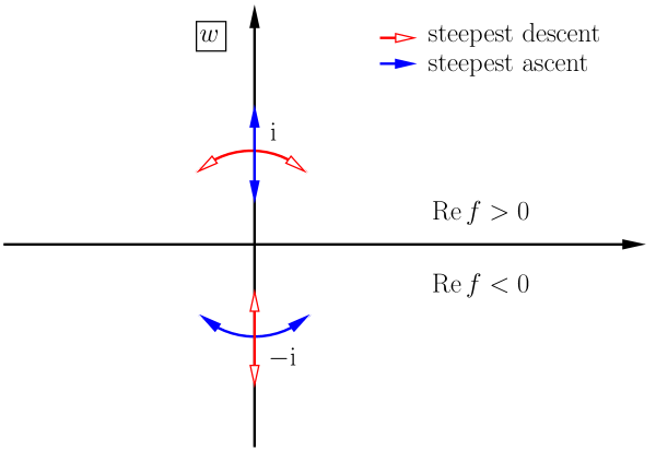
We shall analyse the integrals (B.178) for $\tau\rightarrow+\infty$ ($t\rightarrow-\infty$) by means of the steepest-descent method. This will be enough to understand the behaviour of the correlation function for $t\rightarrow\pm\infty$, since $\langle\sigma_{1}^{-}\sigma_{m+1}^{+}(t)\rangle_{T}=\langle\sigma_{1}^{-}\sigma_{m+1}^{+}(-t)\rangle_{T}^{\ast}$. The reason why $t\rightarrow-\infty$ is easier to analyse than $t\rightarrow+\infty$ is that in the latter case the relevant saddle point coincides with the pole of $b_{m}$ at $w=-{\rm i}$. In fact, the two saddle points, $f^{\prime}(w)=0$, are at $w=\pm{\rm i}$, where $f(\pm{\rm i})=\pm 1$. Hence, the saddle point at $+{\rm i}$ is dominant for $\tau\rightarrow+\infty$, while the saddle point at $-{\rm i}$ dominates for $\tau\rightarrow-\infty$. The saddle-point contours are easily determined in this case. They consist of the unit circle plus the imaginary axis. The steepest descent and steepest ascent directions close to the saddle points are indicated in figure 2.

Refer to caption
Figure 2: Sketch of saddle points and saddle point contours.

According to the usual reasoning of the steepest descent method we can restrict the integration contour to a vicinity of the saddle point at $+{\rm i}$. We may, for instance, choose a semi-circle of unit radius in the upper half plane around the origin, explicitly parameterized as $\theta\mapsto w={\rm i}{\rm e}^{{\rm i}\theta}$, $\theta\in[-\pi/2,\pi/2]$. Then

$$A^{l}_{k}(m){\rm e}^{-\tau}=\int_{-\pi/2}^{\pi/2}{\rm d}\theta\>{\rm e}^{{\rm i}\theta}b_{m}\bigl{(}{\rm i}{\rm e}^{{\rm i}\theta}\bigr{)}\bigl{(}{\rm i}{\rm e}^{{\rm i}\theta}\bigr{)}^{k+l}{\rm e}^{-2\tau\sin^{2}(\theta/2)}+{\cal O}\bigl{(}{\rm e}^{-\tau}\bigr{)}\,.$$ (B.196)

Setting

$$h(\theta)=\sqrt{2}\sin(\theta/2)\,,\quad\mathfrak{b}_{m}(u)=\frac{{\rm e}^{{\rm i}h^{-1}(u)}b_{m}\bigl{(}{\rm i}{\rm e}^{{\rm i}h^{-1}(u)}\bigr{)}}{h^{\prime}\circ h^{-1}(u)}$$ (B.197)

and substituting $u=h(\theta)$ as integration variable in (B.196) we obtain an all-order asymptotic expansion of the integral on the right hand side of (B.196),

$$A^{l}_{k}(m){\rm e}^{-\tau}={\rm i}^{k+l}\sum_{p\geq 0}\frac{\Gamma(p+\frac{1}{2})}{\tau^{p+\frac{1}{2}}(2p!)}\Bigl{[}\partial_{u}^{2p}\mathfrak{b}_{m}(u){\rm e}^{{\rm i}(k+l)h^{-1}(u)}\Bigr{]}_{u=0}+{\cal O}\bigl{(}{\rm e}^{-\tau}\bigr{)}\,.$$ (B.198)

Inserting this into the determinant in the denominator of (120b) and using the multi-linearity of the determinant we obtain

$$\det_{k,l=0,\dots,m}\bigl{\{}A^{l}_{k}(m)\bigr{\}}\sim{\rm e}^{(m+1)\tau}(-1)^{\frac{m(m+1)}{2}}\sum_{p_{0},\dots,p_{m}\geq 0}\biggl{[}\prod_{r=0}^{m}\frac{\Gamma(p_{r}+\frac{1}{2})}{\tau^{p_{r}+\frac{1}{2}}(2p_{r}!)}\partial_{u_{r}}^{2p_{r}}\biggr{]}\\ \times\biggl{(}\prod_{s=0}^{m}\mathfrak{b}_{m}(u_{s}){\rm e}^{{\rm i}s\cdot h^{-1}(u_{s})}\biggr{)}\det_{k,l=0,\dots,m}\bigl{\{}{\rm e}^{{\rm i}kh^{-1}(u_{l})}\bigr{\}}\Bigr{|}_{u_{j}=0}\,,$$ (B.199)

where “$\sim$” means asymptotically equal. The operator

$$\sum_{p_{0},\dots,p_{m}\geq 0}\biggl{[}\prod_{r=0}^{m}\frac{\Gamma(p_{r}+\frac{1}{2})}{\tau^{p_{r}+\frac{1}{2}}(2p_{r}!)}\partial_{u_{r}}^{2p_{r}}\biggr{]}_{u_{j}\rightarrow 0}$$ (B.200)

sends functions $\phi(u_{0},\dots,u_{m})$ that are antisymmetric in any pair of variables $u_{j}$, $u_{k}$ to zero. We may therefore replace the term in the second line of (B.199) by its symmetrized version,

$$\det_{k,l=0,\dots,m}\bigl{\{}A^{l}_{k}(m)\bigr{\}}\sim{\rm e}^{(m+1)\tau}(-1)^{\frac{m(m+1)}{2}}\frac{1}{(m+1)!}\\ \sum_{p_{0},\dots,p_{m}\geq 0}\biggl{[}\prod_{r=0}^{m}\frac{\Gamma(p_{r}+\frac{1}{2})}{\tau^{p_{r}+\frac{1}{2}}(2p_{r}!)}\partial_{u_{r}}^{2p_{r}}\biggr{]}\biggl{[}\prod_{s=0}^{m}\mathfrak{b}_{m}(u_{s})\biggr{]}\Bigl{(}\det_{k,l=0,\dots,m}\bigl{\{}{\rm e}^{{\rm i}kh^{-1}(u_{l})}\bigr{\}}\Bigr{)}^{2}\Bigr{|}_{u_{j}=0}\,.$$ (B.201)

¿From this expression we want to extract the leading term in $\tau$. Many terms under the sum on the right hand side vanish, e.g. the term $p_{0}=p_{1}=\dots=p_{m}$, because the determinants vanish. Non-vanishing terms are generated by the action of the derivatives on the columns of the determinants. The determinants are non-vanishing only if the degrees of the derivatives inside the columns are mutually different. The term of lowest possible degree of the derivatives is generated by $\prod_{r=0}^{m}\partial_{u_{r}}^{2r}$ and corresponds to summands with $p_{r}=r$; $r=0,\dots,m$, modulo permutations. This term can be calculated explicitly,

$$\biggl{[}\prod_{r=0}^{m}\partial_{u_{r}}^{2p_{r}}\biggr{]}\biggl{[}\prod_{s=0}^{m}\mathfrak{b}_{m}(u_{s})\biggr{]}\Bigl{(}\det_{k,l=0,\dots,m}\bigl{\{}{\rm e}^{{\rm i}kh^{-1}(u_{l})}\bigr{\}}\Bigr{)}^{2}\Bigr{|}_{u_{j}=0}\\ =\biggl{[}\prod_{r=0}^{m}\frac{(2r)!\mathfrak{b}_{m}(0){\rm i}^{m}}{(r!)^{2}(h^{\prime}(0))^{m}}\biggr{]}\Bigl{(}\det_{k,l=1,\dots,m}\bigl{\{}k^{l}\bigr{\}}\Bigr{)}^{2}\,.$$ (B.202)

Here the combinatorial factor $\prod_{r=0}^{m}(2r)!/(r!)^{2}$ comes from the application of the Leibniz rule. Since the degrees of the derivatives in (B.201) are connected with the powers of $\tau$, (B.202) corresponds to the leading asymptotics, and we conclude that

$$\det_{k,l=0,\dots,m}\bigl{\{}A^{l}_{k}(m)\bigr{\}}=\biggl{[}\prod_{r=0}^{m}\frac{{\rm e}^{\tau}\Gamma(r+\frac{1}{2})\mathfrak{b}_{m}(0)}{\tau^{r+\frac{1}{2}}(r!)^{2}(h^{\prime}(0))^{m}}\biggr{]}\Bigl{(}\det_{k,l=1,\dots,m}\bigl{\{}k^{l}\bigr{\}}\Bigr{)}^{2}\bigl{(}1+{\cal O}(\tau^{-1})\bigr{)}\\ =\frac{G(m+\frac{3}{2})\bigl{(}-{\rm i}\sqrt{2}\bigr{)}^{m^{2}-1}{\rm e}^{(m+1)(1+{\rm i}c)\tau}}{G(\frac{1}{2})(2\pi)^{m+1}\tau^{\frac{(m+1)^{2}}{2}}}\bigl{(}1+{\cal O}(\tau^{-1})\bigr{)}\,,$$ (B.203)

where $G$ is the Barnes function.

For the numerator in (120b) we have to replace in the $n$th column of the determinant $\mathbf{D}_{n}\rightarrow\mathbf{D}_{m+1}$. This amounts to replacing the column index $k$ in (B.196) and in the following equations by

$$x_{k}^{(n)}=k+\delta_{n,k}(m+1-n)\,.$$ (B.204)

The analysis stays very similar with this minor modification. After a few steps we obtain

$$\det_{k,l=0,\dots,m}\Bigl{\{}A^{l}_{x_{k}^{(n)}}(m)\Bigr{\}}={\rm i}^{m+1-n}\biggl{[}\prod_{r=0}^{m}\frac{{\rm e}^{\tau}\Gamma(r+\frac{1}{2})\mathfrak{b}_{m}(0)}{\tau^{r+\frac{1}{2}}(r!)^{2}(h^{\prime}(0))^{m}}\biggr{]}\det_{k,l=1,\dots,m}\bigl{\{}k^{l}\bigr{\}}\\[4.30554pt] \times\det_{k,l=0,\dots,m}\bigl{\{}-{\rm i}h^{\prime}(0)\partial_{u_{l}}^{l}{\rm e}^{{\rm i}x_{k}^{(n)}h^{-1}(u_{l})}\big{|}_{u_{l}=0}\bigr{\}}\bigl{(}1+{\cal O}(\tau^{-1})\bigr{)}\,.$$ (B.205)

The ratio between (B.203) and (B.205) can be easily calculated explicitly. Then, using (120b), we end up with

$$d_{m+1}^{(n)}=(-{\rm i})^{m+1-n}\binom{m+1}{n}\bigl{(}1+{\cal O}(\tau^{-1})\bigr{)}\,.$$ (B.206)

Inserting this into (117) we obtain the asymptotic formula (B.195) for $Q_{m+1}$. The derivation of the large-$\tau$ asymptotics of $P_{m}$ is similar. ∎

Corollary 2.

For large negative times the ‘prefactor’ in the asymptotic formula (160) for the transverse correlation function behaves as

$$Q_{m+1}(-{\rm i})P_{m}^{\prime}(-{\rm i})-P_{m}(-{\rm i})Q_{m+1}^{\prime}(-{\rm i})=(-1)^{m+1}4^{m}\bigl{(}1+{\cal O}(t^{-1})\bigr{)}\,.$$ (B.207)

The long-time behaviour of the function $u_{m}$ appearing in the exponent in (160) is harder to estimate, since the asymptotic forms of the polynomials $P_{m}$ and $Q_{m+1}$ have high-order zeros at $w={\rm i}$.

C Explicit results for small $m$

We set $\tilde{\tau}=-4Jt$. Even the first few coefficients of the polynomials $P_{m}(z)$ and $Q_{m}(z)$ are already too lengthy to be reproduced here. On the other hand, the combination $W_{m}(\tilde{\tau}):=\bigl{(}Q_{m+1}(-i)P_{m}^{\prime}(-i)-Q^{\prime}_{m+1}(-i)P_{m}(-i)\bigr{)}\,(m=1,2)$ turns out to be relatively simple. We write

$${W}_{m}(\tilde{\tau})=\frac{N_{m}(\tilde{\tau},h)}{D_{m}(\tilde{\tau},h)}\,,\quad m=1,2\,.$$ (C.208)

The denominators and numerators are then explicitly given by

$\displaystyle N_{1}(\tilde{\tau},h)$ $\displaystyle=2e^{\tilde{\tau}}(4iJ\tilde{\tau}^{-1}+h)I_{1}(\tilde{\tau})\,,$ (C.209a)
$\displaystyle D_{1}(\tilde{\tau},h)$ $\displaystyle=-4iJ+h\tau e^{\tilde{\tau}}\bigl{(}I_{0}(\tilde{\tau})-I_{1}(\tilde{\tau})\bigr{)}\,,$ (C.209b)
$\displaystyle N_{2}(\tilde{\tau},h)$ $\displaystyle=\tilde{\tau}^{2}\Bigr{(}e^{2\tilde{\tau}}I_{0}(\tilde{\tau}){}^{2}\left(h^{2}(2\tilde{\tau}-1)-16J^{2}\right)$
$\displaystyle\mspace{72.0mu}+2e^{2\tilde{\tau}}I_{1}(\tilde{\tau})I_{0}(\tilde{\tau})\left(16J^{2}-h^{2}\tilde{\tau}\right)+\left(h-4iJe^{\tilde{\tau}}I_{1}(\tilde{\tau})\right){}^{2}\Bigr{)}\,,$ (C.209c)
$\displaystyle D_{2}(\tilde{\tau},h)$ $\displaystyle=4e^{2\tilde{\tau}}\Bigl{(}h\tilde{\tau}I_{0}(\tilde{\tau}){}^{2}(h\tilde{\tau}+8iJ)$
$\displaystyle\mspace{108.0mu}-2hI_{1}(\tilde{\tau})I_{0}(\tilde{\tau})(h\tilde{\tau}+8iJ)+I_{1}(\tilde{\tau}){}^{2}(4J-ih\tilde{\tau})^{2}\Bigr{)}\,.$ (C.209d)

The final pieces $u_{m}\,(m=1,2)$ are also represented in simple forms,

$\displaystyle u_{1}$ $\displaystyle=4J-4J\frac{\partial}{\partial\tau}\ln D_{1}(\tau,h)\bigr{|}_{\tau=\tilde{\tau}}\,,$ (C.210a)
$\displaystyle u_{2}$ $\displaystyle=-8J\frac{1+\tilde{\tau}}{\tilde{\tau}}-4J\frac{\partial}{\partial\tau}\ln\Bigl{(}D_{2}({\tau},h)\Bigr{)}\Bigr{|}_{\tau=\tilde{\tau}}\,.$ (C.210b)

By substituting these into the formula (160), we obtain

$\displaystyle\bigl{\langle}\sigma_{1}^{-}\sigma_{2}^{+}(t)\bigr{\rangle}_{T}$ $\displaystyle\sim-\frac{J}{T}{\rm e}^{-4J^{2}t^{2}-iht}\frac{4iJ+h\tilde{\tau}}{4iJ\tilde{\tau}}I_{1}(\tilde{\tau})\,,$ (C.211a)
$\displaystyle\bigl{\langle}\sigma_{1}^{-}\sigma_{3}^{+}(t)\bigr{\rangle}_{T}$ $\displaystyle\sim\frac{1}{2}\Bigl{(}-\frac{J}{T}\Bigr{)}^{2}\frac{{\rm e}^{-4J^{2}t^{2}-iht}}{4J^{2}\tilde{\tau}^{2}}\bigl{(}h\tilde{\tau}I_{0}(\tilde{\tau}){}^{2}(h\tilde{\tau}+8iJ)$
$\displaystyle\mspace{90.0mu}-2hI_{1}(\tilde{\tau})I_{0}(\tilde{\tau})(h\tilde{\tau}+8iJ)+I_{1}(\tilde{\tau}){}^{2}(4J-ih\tilde{\tau})^{2}\bigr{)}\,.$ (C.211b)

When $h=0$, these expressions reduce to

$\displaystyle\bigl{\langle}\sigma_{1}^{-}\sigma_{2}^{+}(t)\bigr{\rangle}_{T,h=0}$ $\displaystyle\sim-\frac{J}{T}{\rm e}^{-4J^{2}t^{2}}\frac{I_{1}(\tilde{\tau})}{\tilde{\tau}},$ (C.212a)
$\displaystyle\bigl{\langle}\sigma_{1}^{-}\sigma_{3}^{+}(t)\bigr{\rangle}_{T,h=0}$ $\displaystyle\sim 2\Bigl{(}\frac{J}{T}\Bigr{)}^{2}{\rm e}^{-4J^{2}t^{2}}\Bigl{(}\frac{I_{1}(\tilde{\tau})}{\tilde{\tau}}\Bigr{)}^{2},$ (C.212b)

and the leading order terms in [26] (eq. (6.36)) are recovered if we identify $J_{\text{Perk-Capel}}=2J$.

For larger $m$, we still have difficulties in manipulating huge expressions and present only the result for $m=3$ and $h=0$,

$\displaystyle{W}_{3}(\tilde{\tau})|_{h=0}$ $\displaystyle=-\frac{8e^{\tilde{\tau}}\left(-\tilde{\tau}^{2}I_{0}(\tilde{\tau}){}^{2}+\tilde{\tau}^{2}I_{1}(\tilde{\tau}){}^{2}+\tilde{\tau}I_{1}(\tilde{\tau})I_{0}(\tilde{\tau})+2I_{1}(\tilde{\tau}){}^{2}\right)}{\tilde{\tau}^{3}I_{1}(\tilde{\tau})}\,,$ (C.213a)
$\displaystyle u_{3}|_{h=0}$ $\displaystyle=4J\frac{\partial}{\partial\tau}\Bigl{[}\tau+2\ln\bigl{(}\frac{\tau}{I_{1}(\tau)}\bigr{)}\Bigr{]}_{\tau=\tilde{\tau}}\,,$ (C.213b)
$\displaystyle\bigl{<}\sigma_{1}^{-}\sigma_{4}^{+}(t)\bigr{\rangle}_{T,h=0}$ $\displaystyle\sim 16\Bigl{(}-\frac{J}{T}\Bigr{)}^{3}{\rm e}^{-4J^{2}t^{2}}\frac{I_{1}(\tilde{\tau})}{\tilde{\tau}^{5}}$
$\displaystyle\mspace{72.0mu}\times\Bigl{(}-\tilde{\tau}^{2}I_{0}(\tilde{\tau})^{2}+\tilde{\tau}I_{0}(\tilde{\tau})I_{1}(\tilde{\tau})+(\tilde{\tau}^{2}+2)I_{1}(\tilde{\tau})^{2}\Bigr{)}\,.$ (C.213c)

This is (171) of the main text.

References

  • [1] E. L. Basor and H. Widom, On a Toeplitz determinant identity of Borodin and Okounkov, Integr. Equ. Oper. Theory 37 (2000), 397–401.
  • [2] R. Beals and R. R. Coifman, Scattering and inverse scattering for first order systems, Comm. Pure Appl. Math 37 (1984), 39–90.
  • [3] A. Borodin and A. Okounkov, A Fredholm determinant formula for Toeplitz determinants, Integr. Equ. Oper. Theory 37 (2000), 386–396.
  • [4] U. Brandt and K. Jacoby, Exact results for the dynamics of one-dimensional spin-systems, Z. Phys. B 25 (1976), 181–187.
  • [5] A. P. Calderon, Cauchy integrals on Lipschitz curves and related operators, Proc. Natl. Acad. Sci. USA 74 (1977), 1324–1327.
  • [6] H. W. Capel and J. H. H. Perk, Autocorrelation function of the x-compoment of the magnetization in the one-dimensional XY-model, Physica A 87 (1977), 211–242.
  • [7] F. Colomo, A. G. Izergin, V. E. Korepin, and V. Tognetti, Correlators in the Heisenberg XXO chain as Fredholm determinants, Phys. Lett. A 169 (1992), 243.
  • [8] P. Deift, Integrable operators, Amer. Math. Soc. Transl. (2) 189 (1999), 69–84.
  • [9] P. A. Deift and X. Zhou, Long-time asymptotics for the autocorrelation function of the transverse Ising chain at the critical magnetic field, Singular Limits of Dispersive Waves (N. M. Ercolani et al., ed.), NATO ASI Series, Series B: Physics Vol. 320, Plenum Press, New York, 1994, pp. 183–201.
  • [10] M. Dugave, F. Göhmann, and K. K. Kozlowski, Thermal form factors of the XXZ chain and the large-distance asymptotics of its temperature dependent correlation functions, J. Stat. Mech.: Theor. Exp. (2013), P07010.
  • [11] A. S. Fokas, A. R. Its, and A. V. Kitaev, The isomonodromy approach to matrix models in 2d quantum gravity, Comm. Math. Phys. 147 (1992), 395.
  • [12] J. S. Geronimo and K. M. Case, Scattering theory and polynomials orthogonal on the unit circle, J. Math. Phys. 20 (1979), 299–310.
  • [13] F. Göhmann, M. Karbach, A. Klümper, K. K. Kozlowski, and J. Suzuki, Thermal form-factor approach to dynamical correlation functions of integrable lattice models, J. Stat. Mech.: Theor. Exp. (2017), 113106.
  • [14] F. Göhmann, K. K. Kozlowski, J. Sirker, and J. Suzuki, Equilibrium dynamics of the XX chain, Phys. Rev. B 100 (2019), 155428.
  • [15] F. Göhmann, K. K. Kozlowski, and J. Suzuki, Late-time long-distance asymptotics of the transversal correlation functions of the XX chain in the space-like regime, 2019, preprint, arXiv:1908.11555.
  • [16] A. R. Its, A. G. Izergin, V. E. Korepin, and N. Slavnov, Differential equations for quantum correlations functions, Int. J. Mod. Phys. B 4 (1990), 1003.
  • [17]  , Temperature correlations of quantum spins, Phys. Rev. Lett. 70 (1993), 1704–1706.
  • [18] A. R. Its, A. G. Izergin, V. E. Korepin, and G. G. Varzugin, Large time and distance asymptotics of field correlation function of impenetrable bosons at finite temperature, Physica D 54 (1992), 351.
  • [19] N. Kitanine, K. K. Kozlowski, J. M. Maillet, N. A. Slavnov, and V. Terras, Riemann-Hilbert approach to a generalised sine kernel and applications, Comm. Math. Phys. 291 (2009), 691.
  • [20] V. E. Korepin and N. A. Slavnov, The time dependent correlation function of an impenetrable Bose gas as a Fredholm minor I, Comm. Math. Phys. 129 (1990), 103–113.
  • [21] K. K. Kozlowski, Riemann-Hilbert approach to the time-dependent generalized sine kernel, Adv. Theor. Math. Phys. 15 (2011), 1655.
  • [22] E. H. Lieb, T. Schultz, and D. Mattis, Two soluble models of an antiferromagnetic chain, Ann. Phys. (N.Y.) 16 (1961), 407–466.
  • [23] B. M. McCoy, J. H. H. Perk, and R. E. Shrock, Time-dependent correlation functions of the transverse Ising chain at the critical magnetic field, Nucl. Phys. B 220 (1983), 35.
  • [24] G. Müller and R. E. Shrock, Dynamic correlation functions for one-dimensional quantum-spin systems: New results based on a rigorous approach, Phys. Rev. B 29 (1984), 288.
  • [25] T. Niemeijer, Some exact calculations on a chain of spins $\frac{1}{2}$, Physica 36 (1967), 377.
  • [26] J. H. H. Perk and H. W. Capel, Time-dependent xx-correlation functions in the one-dimensional XY-model, Physica A 89 (1977), 265–303.
  • [27] K. Sakai, Dynamical correlation functions of the XXZ model at finite temperature, J. Phys. A 40 (2007), 7523.
  • [28] L. A. Sakhnovich, Operators which are similar to unitary operators with absolutely continuous spectrum, Funct. Anal. Appl. 2 (1968), 48–60.