Alexander polynomials of simple-ribbon knots

Abstract

This is a revised version of [6]. We revised the diagrams of $10_{42}$, $10_{75}$ in Figure 3, and the values of $l$ of $F(t\,;m,p,l)$ for $10_{42}$, $10_{75}$ and the value of $p$ of $F(t\,;m,p,l)$ for $10_{99}$ in Table 1. In [4], we introduced special types of fusions, so called simple-ribbon fusions on links. A knot obtained from the trivial knot by a finite sequence of simple-ribbon fusions is called a simple-ribbon knot. Every ribbon knot with $\leq 9$ crossings is a simple-ribbon knot. In this paper, we give a formula for the Alexander polynomials of simple-ribbon knots. Using the formula, we determine if a knot with $10$ crossings is a simple-ribbon knot. Every simple-ribbon fusion can be realized by “elementary” simple-ribbon fusions. We call a knot an $m$-simple-ribbon knot if the knot is obtained from the trivial knot by a finite sequence of elementary $m$-simple-ribbon fusions for a fixed positive integer $m$. We provide a condition for a simple-ribbon knot to be both of an $m$-simple-ribbon knot and an $n$-simple-ribbon knot for positive integers $m$ and $n$.

1. Introduction

Knots and links are assumed to be ordered and oriented, and they are considered up to ambient isotopy in an oriented $3$-sphere $S^{3}$. In [4], we introduced special types of fusions, so called simple-ribbon fusions. A ($m$-)ribbon fusion on a link $\ell$ is an $m$-fusion ([3, Definition 13.1.1]) on the split union of $\ell$ and an $m$-component trivial link $\mathcal{O}$ such that each component of $\mathcal{O}$ is attached to a component of $\ell$ by a single band. Note that any knot obtained from the trivial knot by a finite sequence of ribbon fusions is a ribbon knot ([3, Definition 13.1.9]), and that any ribbon knot can be obtained from the trivial knot by ribbon fusions. Here we only define an elementary simple-ribbon fusion. A general simple-ribbon fusion can be realized by elementary simple-ribbon fusions. Refer [4] for precise definition.

Let $\ell$ be a link and $\mathcal{O}=O_{1}\cup\cdots\cup O_{m}$ the $m$-component trivial link which is split from $\ell$. Let $\mathcal{D}=D_{1}\cup\cdots\cup D_{m}$ be a disjoint union of non-singular disks with $\partial D_{i}=O_{i}$ and $D_{i}\cap\ell=\emptyset$ ($i=1,\cdots,m$), and let $\mathcal{B}=B_{1}\cup\cdots\cup B_{m}$ be a disjoint union of disks for an $m$-fusion, called bands, on the split union of $\ell$ and $\mathcal{O}$ satisfying the following (see Figure 1 for example):

• $B_{i}\cap\ell=\partial B_{i}\cap\ell=\{$ a single arc $\}$;

• $B_{i}\cap\mathcal{O}=\partial B_{i}\cap O_{i}=\{$ a single arc $\}$; and

• $B_{i}\cap{\rm int}\>\mathcal{D}=B_{i}\cap{\rm int}\>D_{i+1}=\{$ a single arc of ribbon type $\}$.

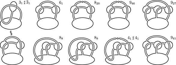
Figure 1. ribbon knots with less than or equal to nine crossings

Let $L$ be a link obtained from the split union of $\ell$ and $\mathcal{O}$ by the $m$-fusion along $\mathcal{B}$, i.e., $L=(\ell\cup\mathcal{O}\cup\partial\mathcal{B})-{\rm int}(\mathcal{B}\cap\ell)-{\rm int}(\mathcal{B}\cap\mathcal{O})$. Then we say that $L$ is obtained from $\ell$ by an elementary ($m$-)simple-ribbon fusion or an elementary ($m$-)SR-fusion (with respect to $\mathcal{D}\cup\mathcal{B}$). If a knot $K$ is obtained from the trivial knot $O$ by a finite sequence of elementary SR-fusions, then we call $K$ a simple-ribbon knot (or an SR-knot). Since an elementary SR-fusion is a ribbon fusion, any SR-knot is a ribbon knot. We also call the trivial knot an SR-knot. As illustrated in Figure 1, all the ribbon knots with $\leq 9$ crossings are SR-knots.

Let $\dot{D}_{i}$ and $\dot{B}_{i}$ be disks and $f:\cup_{i}\left(\dot{D}_{i}\cup\dot{B}_{i}\right)\to S^{3}$ an immersion such that $f(\dot{D}_{i})=D_{i}$ and $f(\dot{B}_{i})=B_{i}$. We denote the arc of ${\rm int}\>D_{i}\cap B_{i-1}$ by $\alpha_{i}$ and let $B_{i,1}$ and $B_{i,2}$ be the subdisks of $B_{i}$ such that $B_{i,1}\cup B_{i,2}=B_{i}$, $B_{i,1}\cap B_{i,2}=\alpha_{i+1}$, and $B_{i,1}\cap\partial D_{i}\neq\emptyset$. Take a point $b_{i}$ on ${\rm int}\>\alpha_{i}$ ($i=1$, $\ldots$, $m$) and an arc $\beta_{i}$ on $D_{i}\cup B_{i,1}$ so that $\beta_{i}\cap(\alpha_{i}\cup\alpha_{i+1})=\partial\beta_{i}=b_{i}\cup b_{i+1}$ and oriented from $b_{i+1}$ to $b_{i}$ (see Figure 2). Then $\beta=\cup_{i}\beta_{i}$ is an oriented simple loop and we call $\beta$ an attendant knot of $\mathcal{D}\cup\mathcal{B}$. Moreover, we denote the pre-images of $\alpha_{i}$ (resp. $b_{i}$) on $\dot{D}_{i}$ and $\dot{B}_{i-1}$ by $\dot{\alpha}_{i}$ and $\ddot{\alpha}_{i}$ (resp. $\dot{b}_{i}$ and $\ddot{b}_{i}$), respectively.

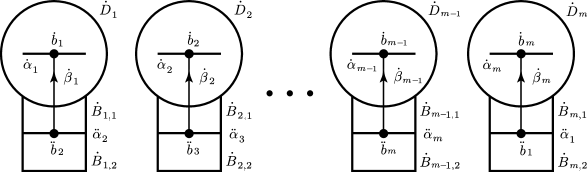
Figure 2.

$\mathcal{D}\cup\mathcal{B}$ is oriented so that induced orientations on boundaries are compatible with the orientation of $\ell$. Then we can see that each band $B_{i}$ intersects with $D_{i+1}$ in two ways, i.e. when we pass through $\alpha_{i+1}$ from $B_{i,2}$ to $B_{i,1}$, we pass through $D_{i+1}$ either from the negative side to the positive side of $D_{i+1}$, or from the positive side to the negative side of $D_{i+1}$. In the former and latter cases, we say that $B_{i}$ is positive and negative, respectively. Then we have the following.

Theorem 1.1.

Let $K$ be a knot obtained from a knot $k$ by an elementary $m$-SR-fusion with an attendant knot $\beta$ and with $p$ positive bands. Let $l=\mathrm{lk}(\beta,k)$ and $\varphi(t\,;m,p,l)=(1-t)^{m}-t^{\,l}(-t)^{p}$. Then we have the following.

(1.1) $$\Delta_{K}(t)\doteq\Delta_{k}(t)\,\varphi(t\,;m,p,l)\,\varphi(t^{-1}\,;m,p,l)$$

Remark. We can also write $\Delta_{K}(t)$ as $\Delta_{k}(t)\,\varphi(t\,;m,p,l)\,\varphi(t\,;m,m\!-\!p,-l)$, i.e.

(1.2) $$\Delta_{K}(t)\doteq\Delta_{k}(t)\,\{(1-t)^{m}-t^{\,l}(-t)^{p}\}\,\{(1-t)^{m}-t^{-l}(-t)^{m-p}\}$$

Corollary 1.2.

Let $K$ be a knot obtained from a knot $k$ by a finite sequence of elementary SR-fusions, i.e., there exists a finite sequence $k=K_{0}$, $K_{1}$, $\ldots$, $K_{N}=K$ of knots such that $K_{i}$ is obtained from $K_{i-1}$ by an elementary $m_{i}$-SR-fusion with an attendant knot $\beta_{i}$ and with $p_{i}$ positive bands $(i=1,\ldots,N)$. Let $l_{i}=\mathrm{lk}(\beta_{i},K_{i-1})$ and $\varphi(t\,;m_{i},p_{i},l_{i})=(1-t)^{m_{i}}-t^{\,l_{i}}(-t)^{p_{i}}$. Then we have the following.

(1.3) $$\Delta_{K}(t)\doteq\Delta_{k}(t)\prod_{i=1}^{N}\varphi(t\,;m_{i},p_{i},l_{i})\,\varphi(t^{-1}\,;m_{i},p_{i},l_{i})$$

As mentioned in the beginning, all the ribbon knots with $\leq 9$ crossings are SR-knots. Using Corollary 1.2, we can determine if a ribbon knot with $10$ crossings is an SR-knot. To do this, we use a value derived from the Alexander polynomial. For a knot $K$, let $\Delta^{\prime}_{K}(t)$ be the polynomial such that $\Delta^{\prime}_{K}(t)\doteq\Delta_{K}(t)$ and $\Delta^{\prime}_{K}(0)\neq 0$. Then define $\delta_{2}(K)$ as $0$ if $|\Delta^{\prime}_{K}(2)|=0$ and as the largest odd factor of $|\Delta^{\prime}_{K}(2)|$ if $|\Delta^{\prime}_{K}(2)|\neq 0$. Note that if $K$ is a simple-ribbon knot, then $\delta_{2}(K)$ is a product of the integers of the form $2^{s}\pm 1$ $(s=0,1,2,\ldots)$ from Corollary 1.2.

Lemma 1.3.

If $K$ is a simple-ribbon knot such that $\delta_{2}(K)=1$, then we have the following for a non-negative integer $n$.

(1.4) $$\Delta^{\prime}_{K}(t)=1~{}~{}\mbox{\rm{or}}~{}~{}(1-6t+11t^{2}-6t^{3}+t^{4})^{n}$$

Proof.

Since $K$ is a simple-ribbon knot, we have the following from Corollary 1.2, where $N$ $(\geq 1)$, $m_{i}$ $(\geq 1)$, $p_{i}$ $(0\leq p_{i}\leq m_{i})$, and $l_{i}$ are integers $(i=1,2,\ldots,N)$.

$\Delta_{K}(t)\doteq\prod_{i=1}^{N}\{(1-t)^{m_{i}}-t^{\,l_{i}}(-t)^{p_{i}}\}\,\{(1-t)^{m_{i}}-t^{-l_{i}}(-t)^{m_{i}-p_{i}}\}$

$\doteq\prod_{i=1}^{N}\{t^{p_{i}+l_{i}}+(-1)^{m_{i}-(p_{i}+1)}(t-1)^{m_{i}}\}\,\{t^{m_{i}-(p_{i}+l_{i})}+(-1)^{p_{i}+1}(t-1)^{m_{i}}\}$

Let $g_{i}(t)=t^{p_{i}+l_{i}}+(-1)^{m_{i}-(p_{i}+1)}(t-1)^{m_{i}}$ and $h_{i}(t)=t^{m_{i}-(p_{i}+l_{i})}+(-1)^{p_{i}+1}(t-1)^{m_{i}}$. Then we have that $\Delta^{\prime}_{K}(2)=2^{q}\prod_{i=1}^{N}g_{i}(2)h_{i}(2)$ for an integer $q$. Since $\delta_{2}(K)=1$, each of $|g_{i}(2)|$ and $|h_{i}(2)|$ is a power of $2$, and thus $2^{-1}=|2^{-1}-1|$, $2=2^{0}+1$, or $1=2^{1}-1$ ($i=1,2,\ldots,N$). Thus, each of $p_{i}+l_{i}$ and $m_{i}-(p_{i}+l_{i})$ is $-1$, $0$, or $1$ for each $i$, and hence $m_{i}=(p_{i}+l_{i})+(m_{i}-(p_{i}+l_{i}))$ is $1$ or $2$, since $m_{i}>0$. Therefore we have that $(g_{i}(2),h_{i}(2),m_{i})=(2^{0}+1,2^{1}-1,1)$, $(2^{1}-1,2^{0}+1,1)$, or $(2^{1}-1,2^{1}-1,2)$. In the first two cases and the last case, we have that $g_{i}(t)h_{i}(t)=\{t^{0}+(t-1)\}\{t^{1}-(t-1)\}=t$ and $g_{i}(t)h_{i}(t)=\{t-(t-1)^{2}\}^{2}=1-6t+11t^{2}-6t^{3}+t^{4}$, respectively. Hence we obtain the conclusion. ∎

Proposition 1.4.

Among the $16$ ribbon knots with $10$ crossings, $10_{42}$, $10_{75}$, $10_{87}$, $10_{99}$, $10_{129}$, $10_{137}$, $10_{140}$, $10_{153}$, and $10_{155}$ are simple-ribbon knots and $10_{3}$, $10_{22}$, $10_{35}$, $10_{48}$, $10_{123}$, $5_{1}\>\sharp\>5_{1}^{*}$, and $5_{2}\>\sharp\>5_{2}^{*}$ are not.

Proof.

The former statement is from Figure 3. To show the latter statement, we consider $\delta_{2}$ for each knot. Since $\delta_{2}(10_{22})=11$, $\delta_{2}(10_{48})=7\times 13=1\times 91$, and $\delta_{2}(5_{1}\>\sharp\>5_{1}^{*})=11\times 11=1\times 121$ from Table 1 and none of $11$, $13$, $91$, and $121$ is $2^{s}\pm 1$ for a non-negative integer $s$, we know that these $3$ knots are not simple-ribbon knots. For the other $4$ knots, we have that $\delta_{2}(10_{3})=\delta_{2}(10_{35})=\delta_{2}(10_{123})=\delta_{2}(5_{2}\>\sharp\>5_{2}^{*})=1$, and the following from Table 1. Hence we know that they are not simple-ribbon knots from Lemma 1.3.

$\Delta^{\prime}_{10_{3}}(t)=6-13t+6t^{2}$,                           $\Delta^{\prime}_{10_{35}}(t)=2-12t+21t^{2}-12t^{3}+2t^{4},$

$\Delta^{\prime}_{10_{123}}(t)=(1-3t+3t^{2}-3t^{3}+t^{4})^{2},$       $\Delta^{\prime}_{5_{2}\>\sharp\>5_{2}^{*}}(t)=4-12t+17t^{2}-12t^{3}+4t^{4}$ ∎

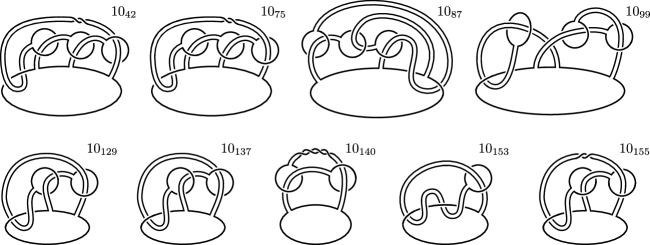
Figure 3.

Note that the above proof of Proposition 1.4 implies that for any ribbon knot $K$ with $\leq 10$ crossings, if $\Delta_{K}(t)$ can be written as equation (1.3), then $K$ is a simple-ribbon knot. However, it does not hold in general.

Theorem 1.5.

For any polynomial $\Delta(t)=\prod_{i=1}^{N}\varphi(t\,;m_{i},p_{i},l_{i})\,\varphi(t^{-1}\,;m_{i},p_{i},l_{i})$, there exists a ribbon knot whose Alexander polynomial is $\Delta(t)$ and which is not a simple-ribbon knot.

If an SR-knot is obtained from the trivial knot by a finite sequence of elementary $m$-SR-fusions for a fixed positive integer $m$, then we call the SR-knot $m$-SR-knot. For example, $8_{9}$ is a $2$-SR-knot and $3_{1}\>\sharp\>3_{1}^{*}$ is a $1$-SR-knot and also a $2$-SR-knot as we can see in Figure 1. It is natural to ask if there exists a simple-ribbon knot which is an $m$-SR-knot and also an $n$-SR-knot for distinct positive integers $m$ and $n$ other than $3_{1}\>\sharp\>3_{1}^{*}$. We give a partial answer to this question using equation (1.3). Let $m$ be a positive integer and $\mathcal{K}_{m}$ the set of non-trivial $m$-SR-knots. Then we have the following.

Theorem 1.6.

If $\mathcal{K}_{m}\cap\mathcal{K}_{n}\neq\emptyset$ for positive integers $m$ and $n$ with $m>n$, then we have either that $(m,n)=(3,1)$, $(3,2)$, or $(2n,n)$.

2. Proofs of Theorem 1.1 and Theorem 1.5

Let $K$ be a knot obtained from a knot $k$ by an elementary $m$-SR-fusion with respect to $\mathcal{D}\cup\mathcal{B}$ with its attendant knot $\beta$. Let $F$ be a Seifert surface for $k$. Here we may take $F$ so that $F\cap\mathcal{D}=\emptyset$. Let $\mathcal{C}=F\cup(\mathcal{D}\cup\mathcal{B})$. We first transform $\mathcal{C}$ into “standard” position and construct a Seifert surface $F_{K}$ for $K$ from $\mathcal{C}$ in standard position. Then, we calculate $\Delta_{K}(t)$ using $F_{K}$.

We may take $F$ so that the intersections with $\mathcal{D}\cup\mathcal{B}$ are only arcs of $\mathrm{int}F$ and $\mathcal{B}$. Then we divide the set of singularities of $\mathrm{int}F\cap B_{i}$ into two: one which consists of $\mathrm{int}F\cap B_{i,1}$, denoted by $\mathcal{S}_{i}$, and the other which consists of $\mathrm{int}F\cap B_{i,2}$, denoted by $\mathcal{T}_{i}$. Thus the set of singularities of $\mathcal{C}$ is $\cup_{i}\alpha_{i}\cup\cup_{i}(\mathcal{S}_{i}\cup\mathcal{T}_{i})$. We say that $\mathcal{C}$ is in standard position if $\mathcal{S}_{1}\cup\cdots\cup\mathcal{S}_{m-1}=\emptyset$ and $\mathcal{T}_{1}\cup\cdots\cup\mathcal{T}_{m}=\emptyset$ (see Figure 9 for example). To transform $\mathcal{C}$ into standard position, we need the following three transformations. Here note that each transformation changes neither $m$, $p$, nor the knot type of $\beta$.

Sliding a disk along a band : Deforming $D_{i+1}$ by deformation retraction into a regular neighborhood of $B_{i}$ and slide $D_{i+1}$ along $B_{i}$ toward $D_{i}$. Here $B_{i+1}$ follows $D_{i+1}$ (see Figure 4 for example). We allow $D_{i+1}\cup B_{i+1}$ to pass through $F$. Then an additional intersection of $B_{i+1}$ and $F$ is created.

Winding a band along $k$ : Winding $B_{i}$ along $k=\partial F$ in a regular neighborhood of $B_{i}\cap k$ either from negative side to positive side or from positive side to negative side (see Figure 5 for example). Here an additional intersection of $B_{i}$ and $F$ is created.

Tubing $F$ : Removing two disks $\delta_{1}$ and $\delta_{2}$ from $\mathrm{int}\,F$ and attatch an annulus $S^{1}\times[1,2]$ so that $S^{1}\times\{i\}=\partial\delta_{i}$ $(i=1,2)$ and the result is orientable (see Figure 6 for example).

Proposition 2.1.

Let $K$ be a knot obtained from a knot $k$ by an elementary $m$-SR-fusion with respect to $\mathcal{D}\cup\mathcal{B}$ with its attendant knot $\beta$. Let $F$ be a Seifert surface for $k$ such that $F\cap\mathcal{D}=\emptyset$ and let $\mathcal{C}\!=\!F\cup(\mathcal{D}\cup\mathcal{B})$. Then we may transform $\mathcal{C}$ into standard position by sliding a disk along a band, winding a band along $k$, and tubing $F$.

Proof.

First if $\mathcal{S}_{1}\cup\cdots\cup\mathcal{S}_{m-1}\neq\emptyset$, then take the smallest index $i$ such that $\mathcal{S}_{i}\neq\emptyset$ and slide $D_{i+1}$ along $B_{i}$ just next to $D_{i}$ so that $\mathcal{S}_{i}=\emptyset$ (See Figure 4 for example). Then slide $D_{j+1}$ along $B_{j}$ inductively just next to $D_{j}$ so that $\mathcal{S}_{j}=\emptyset$ $(j=i+1,\ldots,m-1)$.

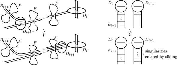
Figure 4.

Next if $\mathcal{T}_{1}\cup\cdots\cup\mathcal{T}_{m}\neq\emptyset$, then take an arbitrary $\mathcal{T}_{i}\neq\emptyset$ and let $t_{1}$, $\ldots$, $t_{p}$ be its singularities which are placed close to $B_{i}\cap k$ on $B_{i}$ in this order. Assume that $B_{i}$ is oriented as from $B_{i}\cap k$ towards $B_{i}\cap D_{i}$ and let $\sigma(t_{j})$ be the signed intersection number of $B_{i}$ and $F$ at $t_{j}$. First wind $B_{i}$ along $k$ depending on $\sigma(t_{j})$ $(j=1,\ldots,p)$. If $\sigma(t_{j})=1$ (resp. $-1$), then wind $B_{i}$ along $k=\partial F$ from negative side to positive side (resp. from positive side to negative side) as illustrated in Figure 5. Here we make these transformations from $j=1$ to $j=p$ in this order, and notice that each transformation creates a new intersection $t^{\prime}_{j}$ with $\sigma(t^{\prime}_{j})=-\sigma(t_{j})$. Then make a tubing $F$ so to erase $t_{j}$ and $t^{\prime}_{j}$ from $j=1$ to $j=p$ in this order as illustrated in Figure 6, and now $\mathcal{C}$ is in standard position. ∎

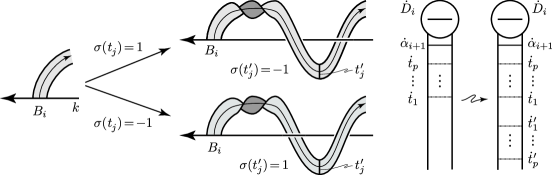
Figure 5.

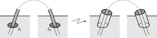
Figure 6.

Proof of Theorem 1.1. Let $F$ be a Seifert surface for $k$ such that $F\cap\mathcal{D}=\emptyset$ and let $\mathcal{C}=F\cup(\mathcal{D}\cup\mathcal{B})$. Here we may assume that $\mathcal{C}$ is in standard position from Proposition 2.1. Thus the set of singularities of $\mathcal{C}$ is $\cup_{i}\alpha_{i}\cup\mathcal{S}_{m}$. Erase $\cup_{i}\alpha_{i}$ and $\mathcal{S}_{m}$ to have a Seifert surface $F_{K}$ for $K$ by orientation preserving cut and deformation as illustrated in the second left of Figure 7 and Figure 8, respectively (see Figure 10 for example of $F_{K}$).

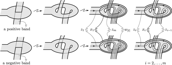
Figure 7.

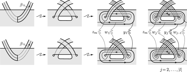
Figure 8.

Take a basis $x_{1}$, $\ldots$, $x_{m}$, $y_{1}$, $\ldots$, $y_{|l|}$, $z_{1}$, $\ldots$, $z_{m}$, $w_{1}$, $\ldots$, $w_{|l|}$, $u_{1}$, $\cdots$, $u_{g}$ of $H_{1}(F_{K};\mathbb{Z})$ as illustrated in Figure 7 and Figure 8 (see Figure 10 for example), where $u_{1}$, $\cdots$, $u_{g}$ is a basis of $H_{1}(F;\mathbb{Z})$. Then we have the following Seifert matrix $M$ with respect to the basis.

$$M\!=\!\left({\begin{array}[]{c|c|c}\!\!O_{(m+|l|)\times(m+|l|)}&P_{(m+|l|)\times(m+|l|)}&O_{(m+|l|)\times\,g\,}\!\!\\ \hline\cr\!\!Q_{(m+|l|)\times(m+|l|)}&*&*\!\!\\ \hline\cr\!\!O_{\,g\,\times(m+|l|)}&*&M^{\prime}\!\!\end{array}}\right)\!=\!\left({\begin{array}[]{c|c|c}\!\!\!O_{(m+|l|)\times(m+|l|)}&\begin{array}[]{c|c}\!\!\!P^{1}_{m\times m}&P^{2}_{m\times|l|}\!\!\!\\ \hline\cr\!\!\!P^{3}_{|l|\times m}&P^{4}_{|l|\times|l|}\!\!\!\end{array}&O_{(m+|l|)\times\,g\,}\!\!\!\\ \hline\cr\begin{array}[]{c|c}\!\!\!Q^{1}_{m\times m}&Q^{2}_{m\times|l|}\!\!\!\\ \hline\cr\!\!\!Q^{3}_{|l|\times m}&Q^{4}_{|l|\times|l|}\!\!\!\end{array}&*&*\\ \hline\cr\!\!\!O_{\,g\,\times(m+|l|)}&*&M^{\prime}\end{array}}\right),$$

where $M^{\prime}$ is a Seifert matrix for $k$, $O_{s\times t}$ is the $s\times t$ zero matrix,

$P^{1}_{m\times m}=(p^{1}_{ij})$ is an $m\times m$ matrix with $p^{1}_{ij}=\mathrm{lk}(x_{i},z_{j}^{+})=\left\{\begin{array}[]{ll}\!\!\!-(\varepsilon_{i}+1)/2&\text{if $i=j$}\\ ~{}\>~{}\>~{}\>~{}\>~{}\varepsilon_{i}&\text{if $i=1$ and $j=m$},\\ &\text{or $2\leq i\leq m$ and $j=i-1$}\\ ~{}\>~{}\>~{}\>~{}\>~{}0&\text{otherwise,}\end{array}\right.$
$P^{2}_{m\times|l|}=(p^{2}_{ij})$ is an $m\times|l|$ matrix with $p^{2}_{ij}=\mathrm{lk}(x_{i},w_{j}^{+})=\left\{\begin{array}[]{ll}~{}\>~{}\>~{}\>~{}\>~{}\varepsilon_{1}{}{}{}{}{}{}&\text{if $i=1$ and $j=|l|$}\\ ~{}\>~{}\>~{}\>~{}\>~{}0{}{}{}{}{}{}&\text{otherwise,}\end{array}\right.$
$P^{3}_{|l|\times m}=(p^{3}_{ij})$ is an $|l|\times m$ matrix with $p^{3}_{ij}=\mathrm{lk}(y_{i},z_{j}^{+})~{}=\left\{\begin{array}[]{ll}~{}\>~{}\>~{}\>~{}\>~{}\varepsilon{}{}{}{}{}{}{}&\text{if $j=m$}\\ ~{}\>~{}\>~{}\>~{}\>~{}0{}{}{}{}{}{}{}&\text{otherwise,}\end{array}\right.$
$P^{4}_{|l|\times|l|}=(p^{4}_{ij})$ is an $|l|\times|l|$ matrix with $p^{4}_{ij}=\mathrm{lk}(y_{i},w_{j}^{+})=\left\{\begin{array}[]{ll}(\varepsilon+1)/2{}{}&\text{if $i=j$}\\ (\varepsilon-1)/2{}{}&\text{if $2\leq i\leq|l|$ and $j=i-1$}\\ ~{}\>~{}\>~{}\>~{}\>~{}0&\text{otherwise,}\end{array}\right.$

if $l\neq 0$, and $P_{m\times m}=P^{1}_{m\times m}$ if $l=0$,
$Q^{1}_{m\times m}=(q^{1}_{ij})$ is an $m\times m$ matrix with $q^{1}_{ij}=\mathrm{lk}(z_{i},x_{j}^{+})=\left\{\begin{array}[]{ll}\!\!\!-(\varepsilon_{i}-1)/2&\text{if $i=j$}\\ ~{}\>~{}\>~{}\>~{}\>~{}\varepsilon_{i}&\text{if $i=m$ and $j=1$},\\ &\text{or $1\leq i\leq m-1$ and $j=i+1$}\\ ~{}\>~{}\>~{}\>~{}\>~{}0&\text{otherwise,}\end{array}\right.$
$Q^{2}_{m\times|l|}=(q^{2}_{ij})$ is an $m\times|l|$ matrix with $q^{2}_{ij}=\mathrm{lk}(z_{i},y_{j}^{+})~{}=\left\{\begin{array}[]{ll}~{}\>~{}\>~{}\>~{}\>~{}\varepsilon{}{}{}{}{}{}{}&\text{if $i=m$}\\ ~{}\>~{}\>~{}\>~{}\>~{}0{}{}{}{}{}{}{}&\text{otherwise,}\end{array}\right.$
$Q^{3}_{|l|\times m}=(q^{3}_{ij})$ is an $|l|\times m$ matrix with $q^{3}_{ij}=\mathrm{lk}(w_{i},x_{j}^{+})=\left\{\begin{array}[]{ll}~{}\>~{}\>~{}\>~{}\>~{}\varepsilon_{1}{}{}{}{}{}{}&\text{if $i=|l|$ and $j=1$}\\ ~{}\>~{}\>~{}\>~{}\>~{}0{}{}{}{}{}{}&\text{otherwise, and}\end{array}\right.$
$Q^{4}_{|l|\times|l|}=(q^{4}_{ij})$ is an $|l|\times|l|$ matrix with $q^{4}_{ij}=\mathrm{lk}(w_{i},y_{j}^{+})=\left\{\begin{array}[]{ll}(\varepsilon-1)/2{}{}&\text{if $i=j$}\\ (\varepsilon+1)/2{}{}&\text{if $1\leq i\leq|l|-1$ and $j=i+1$}\\ ~{}\>~{}\>~{}\>~{}\>~{}\>~{}0&\text{otherwise,}\end{array}\right.$

if $l\neq 0$, and $Q_{m\times m}=Q^{1}_{m\times m}$ if $l=0$, and $\varepsilon=\left\{\begin{array}[]{rl}1&\text{if $l$ is positive}\\ -1&\text{if $l$ is negative}\end{array}\right.$, $\varepsilon_{i}=\left\{\begin{array}[]{rl}1&\text{if $B_{i}$ is positive}\\ -1&\text{if $B_{i}$ is negative}\end{array}\right.$

$(i=1,\ldots,m)$. Letting $a=\displaystyle\frac{\varepsilon+1}{2}$, $b=\displaystyle\frac{\varepsilon-1}{2}$, $a_{i}=\displaystyle\frac{\varepsilon_{i}+1}{2}$, and $b_{i}=\displaystyle\frac{\varepsilon_{i}-1}{2}$, we have the following.

$P\!=\!\bordermatrix{&\!z^{+}_{1}\!&\!z^{+}_{2}\!&\!\cdots\!&\!z^{+}_{m-1}\!&\!z_{m}\!&\!w^{+}_{1}\!&\!w^{+}_{2}\!&\!\cdots\!&\!w^{+}_{|l|-1}\!\!&\!\!w^{+}_{|l|}\!\cr x_{1}&-a_{1}\!\!\!\!&&&&\!\!\!\!\varepsilon_{1}\!\!\!\!&&&&&\!\!\!\!\varepsilon_{1}\!\!\!\!\cr x_{2}&\varepsilon_{2}\!\!\!\!&\!\!\!\!-a_{2}\!\!\!\!&&&&&&&&\cr~{}\vdots&&\!\!\!\!\ddots\!\!\!\!&\!\!\!\!\ddots\!\!\!\!&&&&&&&\cr x_{m-1}&&&\!\!\!\!\ddots\!\!\!\!&\!\!\!\!-a_{m-1}\!\!\!\!&&&&&&\cr x_{m}&&&&\!\!\!\!\varepsilon_{m}\!\!\!\!&\!\!\!\!-a_{m}\!\!\!\!&&&&&\cr y_{1}&&&&&\varepsilon&\!\!\!a\!\!\!&&&&\cr y_{2}&&&&&\varepsilon&\!\!\!b\!\!\!&\!\!\!a\!\!\!&&&\cr~{}\vdots&&&&&\varepsilon&&\!\!\!\ddots\!\!\!&\!\!\!\ddots\!\!\!&&\cr y_{|l|-1}&&&&&\varepsilon&&&\!\!\!\ddots\!\!\!&\!\!\!a\!\!\!&\cr y_{|l|}&&&&&\varepsilon&&&&\!\!\!b\!\!\!&\!\!\!a\!\!\!\cr}$, $Q\!=\!\bordermatrix{&\!x^{+}_{1}\!&\!x^{+}_{2}\!&\!\cdots\!&\!x^{+}_{m-1}\!&\!x_{m}\!&\!y^{+}_{1}\!&\!y^{+}_{2}\!&\!\cdots\!&\!y^{+}_{|l|-1}\!\!&\!\!y^{+}_{|l|}\!\cr z_{1}&-b_{1}\!\!\!\!&\!\!\!\!\varepsilon_{2}\!\!\!\!&&&&&&&&\cr z_{2}&&\!\!\!\!-b_{2}\!\!\!\!&\!\!\!\!\ddots\!\!\!\!&&&&&&&\cr\vdots&&&\!\!\!\!\ddots\!\!\!\!&\!\!\!\!\ddots\!\!\!\!&&&&&&\cr z_{m-1}&&&&\!\!\!\!-b_{m-1}\!\!\!\!&\!\!\!\!\varepsilon_{m}\!\!\!\!&&&&&\cr z_{m}&\!\varepsilon_{1}\!&&&&\!\!\!\!-b_{m}\!\!\!\!&\varepsilon&\varepsilon&\varepsilon&\varepsilon&\varepsilon\cr w_{1}&&&&&&b&a&&&\cr w_{2}&&&&&&&b&a&&\cr\vdots&&&&&&&&\!\!\!\ddots\!\!\!&\!\!\!\ddots\!\!\!&\cr w_{|l|-1}&&&&&&&&&\!\!\!b\!\!\!&a\cr w_{|l|}&\!\varepsilon_{1}\!&&&&&&&&&b\cr}$

Then the Alexander polynomial $\Delta_{K}(t)$ of $K$ is the product of the Alexander polynomial $\Delta_{k}(t)$ of $k$, $|P-t\,Q^{T}|$, and $|Q-t\,P^{T}|$.

Claim 2.2.

We have the following, where $c=a-tb$, $d=b-ta$, $e=\varepsilon(1-t)$, $c_{i}=a_{i}-tb_{i}$, $d_{i}=b_{i}-ta_{i}$, and $e_{i}=\varepsilon_{i}(1-t)$.

$$|\,Q\!-\!tP^{T}|=\displaystyle d^{\,|l|}\prod_{i=1}^{m}(-d_{i})+(-1)^{|l|+m+1}c^{\,|l|}\prod_{i=1}^{m}e_{i}\,,~{}\,~{}\,~{}|P\!-\!t\,Q^{T}|=\displaystyle c^{\,|l|}\prod_{i=1}^{m}(-c_{i})+(-1)^{|l|+m+1}d^{\,|l|}\prod_{i=1}^{m}e_{i}.$$

Proof.  First we calculate $|\,P\!-\!tQ^{T}|$ noticing that $e=c+d$.

If $l=0$, then we have that $|P\!-\!t\,Q^{T}|=\begin{array}[]{|ccccc|}\!-c_{1}\!\!&&&&e_{1}\\[-2.15277pt] \!e_{2}\!&\!\!-c_{2}\!\!\!&&&\\[-4.30554pt] &\!\!\!\ddots\!\!\!&\!\!\ddots\!\!\!&&\\[-6.45831pt] &&\!\!\ddots\!\!\!&\!-c_{m-1}\!\!\!&\\[-2.15277pt] &&&e_{m}&\!\!-c_{m}\!\!\end{array}$ $=\displaystyle c^{\,0}\prod_{i=1}^{m}(-c_{i})+(-1)^{0+m+1}d^{\,0}\prod_{i=1}^{m}e_{i}$.

If $|l|=1$, then we have that

$|P\!-tQ^{T}|=\begin{array}[]{|ccccc|c|}\!-c_{1}\!\!&&&&e_{1}\!\!\!&e_{1}\!\\[-2.15277pt] \!e_{2}\!&\!\!-c_{2}\!\!\!&&&&\\[-4.30554pt] &\!\!\!\ddots\!\!\!&\!\!\ddots\!\!\!&&&\\[-6.45831pt] &&\!\!\ddots\!\!\!&\!-c_{m-1}\!\!\!&&\\[-2.15277pt] &&&e_{m}&\!\!-c_{m}\!\!&\\ \hline\cr&&&&e&c\end{array}=\begin{array}[]{|ccccc|c|}\!-c_{1}\!\!&&&&0\!\!\!&e_{1}\!\\[-2.15277pt] \!e_{2}\!&\!\!-c_{2}\!\!\!&&&&\\[-4.30554pt] &\!\!\!\ddots\!\!\!&\!\!\ddots\!\!\!&&&\\[-6.45831pt] &&\!\!\ddots\!\!\!&\!-c_{m-1}\!\!\!&&\\[-2.15277pt] &&&e_{m}&\!\!-c_{m}\!\!&\\ \hline\cr&&&&d&c\end{array}\,$ $=\displaystyle c^{\,1}\prod_{i=1}^{m}(-c_{i})+(-1)^{1+m+1}d^{\,1}\prod_{i=1}^{m}e_{i}$.

If $|l|>1$, then we have that

$|P\!-tQ^{T}|=\begin{array}[]{|ccccc|ccccc|}\!-c_{1}\!\!&&&&e_{1}\!\!\!&&&&&e_{1}\!\\[-2.15277pt] \!e_{2}\!&\!\!-c_{2}\!\!\!&&&&&&&&\\[-4.30554pt] &\!\!\!\ddots\!\!\!&\!\!\ddots\!\!\!&&&&&&&\\[-6.45831pt] &&\!\!\ddots\!\!\!&\!-c_{m-1}\!\!\!&&&&&&\\[-2.15277pt] &&&e_{m}&\!\!-c_{m}\!\!&&&&&\\ \hline\cr&&&&e&c&&&&\\[-2.15277pt] &&&&e&d&c&&&\\[-5.16663pt] &&&&e&&\ddots&\ddots&&\\[-6.45831pt] &&&&e&&&\ddots&c&\\[-2.15277pt] &&&&e&&&&d&c\!\\[-2.15277pt] \end{array}=\begin{array}[]{|ccccc|ccccc|}\!-c_{1}\!\!&&&&0&&&&&e_{1}\!\!\\[-2.15277pt] \!e_{2}\!&\!\!-c_{2}\!\!\!&&&&&&&&\\[-4.30554pt] &\!\!\!\ddots\!\!\!&\!\!\ddots\!\!\!&&&&&&&\\[-6.45831pt] &&\!\!\ddots\!\!\!&\!-c_{m-1}\!\!\!&&&&&&\\[-2.15277pt] &&&e_{m}&\!\!-c_{m}\!\!&&&&&\\ \hline\cr&&&&d&c&&&&\\[-2.15277pt] &&&&0&d&c&&&\\[-5.16663pt] &&&&0&&\ddots&\ddots&&\\[-6.45831pt] &&&&0&&&\ddots&c&\\[-2.15277pt] &&&&0&&&&d&c\!\!\\[-2.15277pt] \end{array}\,$

$=\displaystyle c^{\,|l|}\prod_{i=1}^{m}(-c_{i})+(-1)^{|l|+m+1}d^{\,|l|}\prod_{i=1}^{m}e_{i}$.

Next we calculate $|\,Q\!-\!tP^{T}|$ noticing that $e=c+d$.

If $l=0$, then we have that $|Q-t\,P^{T}|=\begin{array}[]{|ccccc|}\!\!-d_{1}\!\!&e_{2}\!\!\!&&&\\[-4.30554pt] &\!\!-d_{2}\!\!\!\!\!&\ddots\!\!&&\\[-5.16663pt] &&\ddots\!\!&\ddots\!\!&\\[-2.15277pt] &&&\!\!\!\!-d_{m-1}\!\!\!&e_{m}\\[-2.15277pt] e_{1}\!\!\!&&&&\!\!\!-d_{m}\!\!\end{array}=\displaystyle d^{\,0}\prod_{i=1}^{m}(-d_{i})+(-1)^{0+m+1}c^{\,0}\prod_{i=1}^{m}e_{i}$.

If $|l|=1$, then we have that

$|\,Q\!-tP^{T}|=\begin{array}[]{|ccccc|c|}\!\!-d_{1}\!\!&e_{2}\!\!\!&&&&\\[-2.15277pt] &\!\!-d_{2}\!\!\!\!\!&\ddots\!\!&&&\\[-5.16663pt] &&\ddots\!\!&\ddots\!\!&&\\[-2.15277pt] &&&\!\!\!\!-d_{m-1}\!\!\!&e_{m}&\\[-1.29167pt] e_{1}\!\!\!&&&&\!\!\!-d_{m}\!\!&e\\ \hline\cr e_{1}\!\!\!&&&&&d\\[-2.15277pt] \end{array}=\begin{array}[]{|ccccc|c|}\!\!-d_{1}\!\!&e_{2}\!\!\!&&&&\\[-2.15277pt] &\!\!-d_{2}\!\!\!\!\!&\ddots\!\!&&&\\[-5.16663pt] &&\ddots\!\!&\ddots\!\!&&\\[-2.15277pt] &&&\!\!\!\!-d_{m-1}\!\!\!&e_{m}&\\[-1.29167pt] 0&&&&\!\!\!-d_{m}\!\!&c\\ \hline\cr e_{1}\!\!\!&&&&&d\\[-2.15277pt] \end{array}$ $=\displaystyle d^{\,1}\prod_{i=1}^{m}(-d_{i})+(-1)^{1+m+1}c^{\,1}\prod_{i=1}^{m}e_{i}$.

If $|l|>1$, then we have that

$|\,Q\!-tP^{T}|=\begin{array}[]{|ccccc|ccccc|}\!\!-d_{1}\!\!&e_{2}\!\!\!&&&&&&&&\\[-2.15277pt] &\!\!-d_{2}\!\!\!\!\!&\ddots\!\!&&&&&&&\\[-5.16663pt] &&\ddots\!\!&\ddots\!\!&&&&&&\\[-2.15277pt] &&&\!\!-d_{m-1}\!\!\!&e_{m}&&&&&\\[-1.29167pt] e_{1}\!\!\!&&&&\!\!\!-d_{m}\!\!&e&e&\cdots&e&e\\ \hline\cr&&&&&d&c&&&\\[-2.15277pt] &&&&&&d&\ddots&&\\[-5.16663pt] &&&&&&&\ddots&\ddots&\\[-2.15277pt] &&&&&&&&d&c\\[-2.15277pt] e_{1}\!\!\!&&&&&&&&&d\\[-2.15277pt] \end{array}=\begin{array}[]{|ccccc|ccccc|}\!\!-d_{1}\!\!&e_{2}\!\!\!&&&&&&&&\\[-2.15277pt] &\!\!-d_{2}\!\!\!\!\!&\ddots\!\!&&&&&&&\\[-5.16663pt] &&\ddots\!\!&\ddots\!\!&&&&&&\\[-2.15277pt] &&&\!\!-d_{m-1}\!\!\!&e_{m}&&&&&\\[-1.29167pt] 0&&&&\!\!\!-d_{m}\!\!&c&0&\cdots&0&0\\ \hline\cr&&&&&d&c&&&\\[-2.15277pt] &&&&&&d&\ddots&&\\[-5.16663pt] &&&&&&&\ddots&\ddots&\\[-2.15277pt] &&&&&&&&d&c\\[-2.15277pt] e_{1}\!\!\!&&&&&&&&&d\\[-2.15277pt] \end{array}$

$=\displaystyle d^{\,|l|}\prod_{i=1}^{m}(-d_{i})+(-1)^{|l|+m+1}c^{\,|l|}\prod_{i=1}^{m}e_{i}$.

$\Box$

Now we calculate the Alexander polynomial $\Delta_{K}(t)$ of $K$ diving the case into two depending on the value of $l$; $l\geq 0$ or $l<0$. Here note the following.

$${\begin{array}[]{|c||c|c|c|c|c|}\hline\cr\varepsilon&a&b&c&d&e\\ \hline\cr 1&1&0&1&-t&1-t\\ \hline\cr-1&0&-1&t&-1&-(1-t)\\ \hline\cr\end{array}~{}\;~{}\;~{}\;~{}\begin{array}[]{|c||c|c|c|c|c|}\hline\cr\varepsilon_{i}&a_{i}&b_{i}&c_{i}&d_{i}&e_{i}\\ \hline\cr 1&1&0&1&-t&1-t\\ \hline\cr-1&0&-1&t&-1&-(1-t)\\ \hline\cr\end{array}}$$

Case $l\geq 0$ : From the above table, we have the following;

$|P-t\,Q^{T}|=\displaystyle c^{\,|l|}\prod_{i=1}^{m}(-c_{i})+(-1)^{|l|+m+1}d^{\,|l|}\prod_{i=1}^{m}e_{i}$

$=1^{\,l}\,(-1)^{p}(-t)^{m-p}+(-1)^{l+m+1}(-t)^{\,l}(-1)^{m-p}(1-t)^{m}$ $=(-1)^{1-p}\,\{t^{\,l}(1-t)^{m}-(-t)^{m-p}\}$

$|Q-t\,P^{T}|=\displaystyle d^{\,|l|}\prod_{i=1}^{m}(-d_{i})+(-1)^{|l|+m+1}c^{\,|l|}\prod_{i=1}^{m}e_{i}$

$=(-t)^{\,l}\,t^{\,p}\,1^{m-p}+(-1)^{l+m+1}1^{\,l}\,(-1)^{m-p}(1-t)^{m}$ $=(-1)^{l+1-p}\,\{(1-t)^{m}-t^{\,l}(-t)^{p}\}$

Case $l<0$ : From the above table, we have the following;

$|P-t\,Q^{T}|=\displaystyle c^{\,|l|}\prod_{i=1}^{m}(-c_{i})+(-1)^{|l|+m+1}d^{\,|l|}\prod_{i=1}^{m}e_{i}$

$=t^{-l}\,(-1)^{p}(-t)^{m-p}+(-1)^{-l+m+1}(-1)^{-l}(-1)^{m-p}(1-t)^{m}$ $=(-1)^{1-p}\,\{(1-t)^{m}-t^{-l}(-t)^{m-p}\}$

$|Q-t\,P^{T}|=\displaystyle d^{\,|l|}\prod_{i=1}^{m}(-d_{i})+(-1)^{|l|+m+1}c^{\,|l|}\prod_{i=1}^{m}e_{i}$

$=(-1)^{-l}\,t^{\,p}\,1^{m-p}+(-1)^{-l+m+1}t^{-l}\,(-1)^{m-p}(1-t)^{m}$ $=(-1)^{-l+1-p}\,\{t^{-l}(1-t)^{m}-(-t)^{p}\}$

In both cases, we obtain that $\Delta_{K}(t)\doteq\Delta_{k}(t)\,\{(1-t)^{m}-t^{\,l}(-t)^{p}\}\,\{(1-t)^{m}-t^{-l}(-t)^{m-p}\}$, and thus we complete the proof.

$\Box$

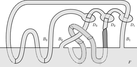
Figure 9.

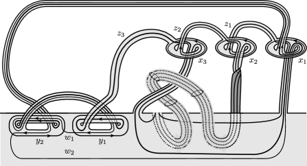
Figure 10.

Proof of Theorem 1.5. For each $i$ $(1\leq i\leq N)$, we can construct a simple-ribbon knot $k_{i}$ with $\Delta_{k_{i}}(t)=\varphi(t\,;m_{i},p_{i},l_{i})\,\varphi(t^{-1}\,;m_{i},p_{i},l_{i})$ by following the proof of Theorem 1.1 (see also Figure 9). Let $K^{\ast}$ be the connected sum of $k_{1}$, $k_{2}$, $\ldots$, $k_{N}$. Then $K^{\ast}$ is a simple-ribbon knot such that $\Delta_{K^{\ast}}(t)=\Delta(t)$. Let $\mathcal{D}\cup\mathcal{B}$ be the set of disks and bands which gives the SR-fusion on the trivial knot $\mathcal{O}=\partial D_{0}$ producing $K^{\ast}$. Take a $3$-ball $H$ which is a small neighborhood of a point of $\mathcal{O}-\mathcal{B}$ and a trivial knot $\rho$ in $H$ which intersects $D_{0}$ twice so that $\mathrm{lk}(\rho,\mathcal{O})=2$. Let $V^{\ast}$ be the closure of $S^{3}-N(\rho;S^{3})$. Since $\rho$ is the trivial knot, $V^{\ast}$ is an unknotted torus which contains $K^{\ast}$ with $w_{V^{\ast}}(K^{\ast})=2$, where $w_{V^{\ast}}(K^{\ast})$ is the absolute value of the algebraic intersection number of $K^{\ast}$ with a meridian disk of $V^{\ast}$.

Let $V$ be a tubular neighborhood of the Kinoshita-Terasaka knot $\kappa$ and $f$ a faithful homeomorphism of $V^{\ast}$ onto $V$, i.e. $f$ maps the preferred longitude of $\partial V^{\ast}$ onto the preferred longitude of $\partial V$. Since $\Delta_{\kappa}(t)=1$, we obtain that $\Delta_{K}(t)=\Delta_{K^{\ast}}(t)\,\Delta_{\kappa}(t^{2})$ $=\Delta_{K^{\ast}}(t)=\Delta(t)$ for $K=f(K^{\ast})$ by Proposition 8.23 of [1]. Since $f$ is faithful and both of $K^{\ast}$ and $\kappa$ are ribbon knots, $K$ is also a ribbon knot by Lemma 3 of [9]. On the other hand, as $w_{V}(K)=w_{V^{\ast}}(K^{\ast})=2$ and $\kappa$ is a non-trivial knot, $K$ is not a simple ribbon knot by Corollary 1.8 of [5].

$\Box$

3. Proof of Theorem 1.6

Note that if $K$ is a knot of $\mathcal{K}_{m}$, then $\mathrm{det}(K)=|\Delta_{K}(-1)|=(2^{\,m}-1)^{a}(2^{\,m}+1)^{b}$ for some non-negative integers $a$ and $b$ by Corollary 1.2. Moreover if $K$ is also a knot of $\mathcal{K}_{n}$, then $\mathrm{det}(K)=(2^{\,n}-1)^{c}(2^{\,n}+1)^{d}$ for some non-negative integers $c$ and $d$, and thus the set of prime factors of $(2^{\,m}-1)^{a^{\prime}}(2^{\,m}+1)^{b^{\prime}}$ and $(2^{\,n}-1)^{c^{\prime}}(2^{\,n}+1)^{d^{\prime}}$ coinside, where $i^{\prime}={\rm min}(i,1)$ for $a$, $b$, $c$, and $d$.

Let $P(x)$ be the set of prime factors of an integer $x>1$, and $(y,z)$ the greatest common divisor of positive integers $y$ and $z$. Note that if $P(y)=P(z)$ and $(y,z)=w$, then we have that $P(y)=P(z)=P(w)$. Here we prepare several lemmas, the first one of which is the theorem by P. Mihăilescu (the Catalan conjecture).

Lemma 3.1.

([7, Theorem 5]) The following equation has no other integer solutions but $3^{2}-2^{3}=1$.

(3.1) $$x^{u}-y^{v}=1~{}(x>0,y>0,u>1,v>1)$$

Lemma 3.2.

([2, Theorem 1]) Let $A$, $m$, and $n$ be integers such that $A>1$ and $m>n\geq 1$. Then $P(A^{m}-1)=P(A^{n}-1)$ if and only if $m=2$, $n=1$, and $A=2^{l}-1$ for an integer $l>0$.

Lemma 3.3.

Let $A$ be an integer such that $A>1$. Then the followings hold.

• $P(A^{p}+1)=P(A+1)$ for an odd integer $p$ $(>1)$ if and only if $p=3$ and $A=2$.

• $P(A^{q}-1)=P(A+1)$ for an even integer $q$ $(>0)$ if and only if $q=2$ and $A=2^{l}+1$ for an integer $l\geq 0$.

Proof.

Since the if parts are easy to be checked, we only show the only if parts.

(1) First the following equation holds, since $p$ is odd.

(3.2) $$B=\displaystyle\frac{A^{p}+1}{A+1}=A^{p-1}-A^{p-2}+\cdots-A+1=\displaystyle\sum_{i=0}^{p-2}\binom{p}{i}(A+1)^{p-i-1}(-1)^{i}+p$$

If $p$ is prime, then we have that $(B,A+1)=(A+1,p)=p$ from equation (3.2), and thus that $P(B)=\{p\}$, since $P(B)\subset P(A^{p}+1)=P(A+1)$. Moreover, we have that $B\equiv p$ $($mod $p^{2})$ also from equation (3.2), since $A+1\equiv 0$ $($mod $p)$, $\binom{p}{p-2}\equiv 0$ $($mod $p)$. Hence we obtain that $B=p$. If $p>3$, then we also have that

(3.3) $$B=A^{p-1}-A^{p-2}+\cdots-A+1=A(A-1)(A^{p-3}+A^{p-5}+\cdots+1)+1>A(A-1)\displaystyle\frac{p-1}{2}+1\geq p,$$

since $A\geq 2$. However then it contradicts that $B=p$. Therefore we have that $p=3$. Then we have that $A^{2}-A+1=B=p=3$ from equation (3.2), and thus that $A=2$, since $A>1$, which completes the proof.

If $p$ is not prime, then let $p^{\prime}$ be a prime factor of $p$, and let $p=p^{\prime}r$ and $B=A^{r}$. Since $r$ and $p^{\prime}$ are odd, we have that $A+1$ divides $A^{r}+1=B+1$ and that $B+1$ divides $B^{p^{\prime}}+1$. Hence we have that $P(A+1)\subset P(B+1)\subset P(B^{p^{\prime}}+1)=P(A^{p}+1)$, since $B^{p^{\prime}}=A^{p}$. Hence we have that $P(B^{p^{\prime}}+1)=P(B+1)$, since $P(A^{p}+1)=P(A+1)$. Thus from the previous case, we have that $p^{\prime}=3$ and $B=A^{r}=2$, and thus $A=2$ and $r=1$. However then, we have that $p=p^{\prime}r=3$, which contradicts that $p$ is not prime.

(2) Since $q$ is even, we have that $q\geq 2$. Hence we have that $P(A-1)\subset P(A^{q}-1)=P(A+1)$, and thus that $P(A^{2}-1)=P((A-1)(A+1))=P(A+1)=P(A^{q}-1)$. Thus we have that $q=2$ from Lemma 3.2. If $A\neq 2=2^{0}+1$, then we have that $A-1>1$ and thus that $A+1$ and $A-1$ are not coprime, since $P(A-1)\subset P(A+1)$. Hence we have that $(A+1,A-1)=(A-1,2)=2$, since $A+1=(A-1)+2$. Therefore we obtain that $A-1=2^{l}$ for $l>0$, which completes the proof. ∎

Using Lemma 3.1 and Lemma 3.3, we show the following.

Proposition 3.4.

Let $A$, $m$, and $n$ be integers such that $A>1$ and $m$, $n\geq 1$. Then we have the following.

• $P(A^{m}+1)=P(A^{n}+1)$ $(m>n)$ if and only if $m=3$, $n=1$, and $A=2$;

• $P(A^{m}+1)=P(A^{n}-1)$ if and only if one of the following holds.

  • $m=1$, $n=1$, and $A=3\,;$

  • $m=3$, $n=2$, and $A=2\,;$

  • $m=2$, $n=4$, and $A=3\,;$ and

  • $m=1$, $n=2$, and $A=2^{l}+1$ for an integer $l\geq 0$.

Proof.

First we have the following for indeterminate $X$ and positive integers $s$, $t$, and $q$ and a non-negative integer $r$ such that $s=qt+r$.

(3.4) $$X^{s}\pm 1=(X^{t}+1)(X^{s-t}-X^{s-2t}+\cdots-(-1)^{q}X^{s-qt})+(-1)^{q}X^{r}\pm 1$$

(3.5) $$X^{s}+1=(X^{t}-1)(X^{s-t}+X^{s-2t}+\cdots+X^{s-qt})+X^{r}+1~{}\ \ \ \ \ \ \ ~{}$$

Let $g=(m,n)$. Then we have the following.

Claim 3.5.

$(A^{m}+1,A^{n}+1),(A^{m}+1,A^{n}-1)=1$, $2$ or $A^{g}+1$.

Proof.

For positive integers $c_{0}$ and $c_{1}$, let $(c_{0},c_{1})=(c_{1},c_{2})=\cdots=(c_{N-1},c_{N})=c_{N}$ be the sequence obtained by the Euclidian algorithm. Then letting $c_{i}=q_{i+1}c_{i+1}+q_{i+2}$, we also have the following from equations (3.4) and (3.5).

(3.6) $$A^{c_{N-1}}\pm 1=(A^{c_{N}}+1)(A^{c_{N-1}-c_{N}}-A^{c_{N-1}-2c_{N}}+\cdots-(-1)^{q}A^{c_{N-1}-{q_{N}}c_{N}})+(-1)^{q_{N}}A^{0}\pm 1$$

(3.7) $$A^{c_{N-1}}+1=(A^{c_{N}}-1)(A^{c_{N-1}-c_{N}}+A^{c_{N-1}-2c_{N}}+\cdots+A^{c_{N-1}-{q_{N}}c_{N}})+A^{0}+1~{}\ \ \ \ \ \ \ \ ~{}\$$

Hence by letting $(c_{0},c_{1})=(m,n)$ or $(n,m)$, we have that $(A^{m}+1,A^{n}+1)$, $(A^{m}+1,A^{n}-1)$ is either $A^{g}+1$ or $(A^{g}\pm 1,2)$, which induces the conclusion. ∎

Since the if parts are easy to be checked, we only show the only if parts.

(1) Since $P(A^{m}+1)=P(A^{n}+1)$, we have that $A^{m}+1$ and $A^{n}+1$ are not coprime, and thus that $(A^{m}+1,A^{n}+1)=2$ or $A^{g}+1$ from Claim 3.5. In the former case, we have that $P(A^{m}+1)=P(A^{n}+1)=P(2)=\{2\}$. Thus, $A^{m}+1=2^{k}$ and $A^{n}+1=2$ for $k>1$, since $m>n$. However then, we have that $A=1$, which contradicts that $A>1$. In the latter case, we have that $P(A^{m}+1)=P(A^{n}+1)=P(A^{g}+1)$ and that $m=gM$ with an odd integer $M$ from equation (3.4). If $M=1$, then $m=g$, which contradicts that $m>n$. Thus $M$ is odd and $M>1$. Then we have that $M=3$ and $A^{g}=2$ by Lemma 3.3 (1), and thus that $A=2$, $g=1$, $m=gM=3$. Hence we have that $n=g=1$, since $m>n$, which completes the proof.

(2) Since $P(A^{m}+1)=P(A^{n}-1)$, we have that $A^{m}+1$ and $A^{n}-1$ are not coprime, and thus that $(A^{m}+1,A^{n}-1)=2$ or $A^{g}+1$ from Claim 3.5. In the former case, we have that $P(A^{m}+1)=P(A^{n}-1)=P(2)=\{2\}$, and thus that $A^{m}+1=2$ or $A^{n}-1=2$. If $A^{m}+1=2$, then $A^{m}=1$, which contradicts that $A>1$. If $A^{m}+1=2^{k}$ $(k>1)$ and $A^{n}-1=2$, then we have that $A=3$ and $n=1$, and thus that $A^{m}+1=3^{m}+1=2^{k}$ $(k>1)$. Then by Lemma 3.1, we have that $m=1$, and thus obtain condition (i).

In the latter case, we have that $P(A^{m}+1)=P(A^{n}-1)=P(A^{g}+1)$ and that $m=gM$ with an odd integer $M$ from equation (3.4). Consider the case where $M>1$. Then we have that $M=3$ and $A^{g}=2$ by Lemma 3.3 (1), and thus that $A=2$, $g=1$, $m=gM=3$. Since $A^{m}+1=2^{3}+1=9$, and thus $P(2^{n}-1)=P(9)=\{3\}$ and $(A^{m}+1,A^{n}-1)=(9,2^{n}-1)=3$, we have that $2^{n}-1=3$ and thus that $n=2$. Therefore we obtain condition (ii).

Next consider the case where $M=1$, i.e., $m=g$. Hence let $n=mq$ $(q\geq 1)$ and $D=A^{m}$. Thus we have that $P(D+1)=P(D^{q}-1)$ and that $(D+1,D^{q}-1)=D+1$. Therefore $q$ is even, since otherwise $D+1$ does not divide $D^{q}-1$. Then we have that $q=2$ and $D=2^{l}+1$ for $l\geq 0$ by Lemma 3.3 (2). If $m>1$ and $l>1$, then the equation $A^{m}=2^{l}+1$ has the unique solution $(A,m,l)=(3,2,3)$ by Lemma 3.1, and thus we obtain condition (iii). If $m=1$, then we have that $n=mq=2$ and $A=2^{l}+1$ for $l\geq 0$, i.e., condition condition (iv). If $l=0$ (resp. $1$), then we have that $A=2$ (resp. $A=3$) and $m=1$, and thus that condition (iv). ∎

Now using Proposition 3.4 and Lemma 3.2 we obtain the following.

Lemma 3.6.

Let $p$, $q$, $r$, $s$, $M$, $N$ be positive integers with $M\neq N$. Then we have the following.

• $(2^{M}-1)^{p}\neq(2^{N}-1)^{r}$.

• If $(2^{M}+1)^{q}=(2^{N}+1)^{s}$ $(M>N)$, then $M=3$, $N=1$, and $s=2q$.

• If $(2^{M}+1)^{q}=(2^{N}-1)^{r}$, then $M=3$, $N=2$, $r=2q$ or $M=1$, $N=2$, $q=r$.

• $(2^{M}-1)^{p}(2^{M}+1)^{q}\neq(2^{N}-1)^{r}(2^{N}+1)^{s}$

• If $(2^{M}-1)^{p}(2^{M}+1)^{q}=(2^{N}-1)^{r}$, then $2M=N$, $p=q=r$.

• If $(2^{M}-1)^{p}(2^{M}+1)^{q}=(2^{N}+1)^{r}$, then $M=1$, $N=3$, $q=2r$.

Proof.

Note that if positive integers $X$, $Y$ and non-negative integers $p$, $q$ satisfies the equation $X^{p}=Y^{q}$, then $P(X)=P(Y)$. The first three statements are obtained by Lemma 3.2, Proposition 3.4 (1), and Proposition 3.4 (2), respectively. For the last three statements, note that $P((2^{M}-1)^{p}(2^{M}+1)^{q})=P(2^{2M}-1)$. Therefore (4) and (5) are obtained by Lemma 3.2, and (6) is obtained by Proposition 3.4 (2). ∎

Proof of Theorem 1.6. Let $K$ be a knot of $\mathcal{K}_{m}\cap\mathcal{K}_{n}$. Then we have that $\mathrm{det}(K)=(2^{\,m}-1)^{a}(2^{\,m}+1)^{b}=(2^{\,n}-1)^{c}(2^{\,n}+1)^{d}$ for some non-negative integers $a$, $b$, $c$, and $d$ by Corollary 1.2. Thus we obtain the conclusion by Lemma 3.6.

$\Box$

Table 1. Ribbon knots with up to 10 crossings, where $F(t\,;m,p,l)=\varphi(t\,;m,p,l)\,\varphi(t^{-1}\,;m,p,l)$

$K$	simple-ribbon	$\delta_{2}(K)$	det(K)		$\Delta^{\prime}_{K}(t)$
$6_{1}$	$\bigcirc$	0	9	$F(t;2,0,0)=$	$2\!\!-\!\!5t+2t^{2}$
$8_{8}$	$\bigcirc$	5	25	$F(t;2,1,-1)=$	$2\!\!-\!\!6t+9t^{2}\!\!-\!\!6t^{3}+2t^{4}$
$8_{9}$	$\bigcirc$	7	25	$F(t;2,2,1)=$	$1\!\!-\!\!3t+5t^{2}\!\!-\!\!7t^{3}+5t^{4}\!\!-\!\!3t^{5}+t^{6}$
$8_{20}$	$\bigcirc$	9	9	$F(t;2,1,0)=$	$1\!\!-\!\!2t+3t^{2}\!\!-\!\!2t^{3}+t^{4}$
$9_{27}$	$\bigcirc$	5	49	$F(t;3,1,0)=$	$1\!\!-\!\!5t+11t^{2}\!\!-\!\!15t^{3}+11t^{4}\!\!-\!\!5t^{5}+t^{6}$
$9_{41}$	$\bigcirc$	7	49	$F(t;3,0,0)=$	$3\!\!-\!\!12t+19t^{2}\!\!-\!\!12t^{3}+3t^{4}$
$9_{46}$	$\bigcirc$	0	9	$F(t;2,0,0)=$	$2\!\!-\!\!5t+2t^{2}$
$10_{3}$	$\times$	1	25		$6\!\!-\!\!13t+6t^{2}$
$10_{22}$	$\times$	11	49		$2\!\!-\!\!6t+10t^{2}\!\!-\!\!13t^{3}+10t^{4}\!\!-\!\!6t^{5}+2t^{6}$
$10_{35}$	$\times$	1	49		$2\!\!-\!\!12t+21t^{2}\!\!-\!\!12t^{3}+2t^{4}$
$10_{42}$	$\bigcirc$	9	81	$F(t;3,2,-1)=$	$1\!\!-\!\!7t+19t^{2}\!\!-\!\!27t^{3}+19t^{4}\!\!-\!\!7t^{5}+t^{6}$
$10_{48}$	$\times$	91	49		$1\!\!-\!\!3t+6t^{2}\!\!-\!\!9t^{3}+11t^{4}\!\!-\!\!9t^{5}+6t^{6}\!\!-\!\!3t^{7}+t^{8}$
$10_{75}$	$\bigcirc$	9	81	$F(t;3,3,-1)=$	$1\!\!-\!\!7t+19t^{2}\!\!-\!\!27t^{3}+19t^{4}\!\!-\!\!7t^{5}+t^{6}$
$10_{87}$	$\bigcirc$	0	81	$F(t;3,2,-1)=$	$2\!\!-\!\!9t+18t^{2}\!\!-\!\!23t^{3}+18t^{4}\!\!-\!\!9t^{5}+2t^{6}$
$10_{99}$	$\bigcirc$	81	81	$F(t;1,1,1)F(t;2,1,0)=$	$1\!\!-\!\!4t+10t^{2}\!\!-\!\!16t^{3}+19t^{4}\!\!-\!\!16t^{5}+10t^{6}\!\!-\!\!4t^{7}+t^{8}$
$10_{123}$	$\times$	1	121		$1\!\!-\!\!6t+15t^{2}\!\!-\!\!24t^{3}+29t^{4}\!\!-\!\!24t^{5}+15t^{6}\!\!-\!\!6t^{7}+t^{8}$
$10_{129}$	$\bigcirc$	5	25	$F(t;2,1,1)=$	$2\!\!-\!\!6t+9t^{2}\!\!-\!\!6t^{3}+2t^{4}$
$10_{137}$	$\bigcirc$	1	25	$F(t;2,0,1)=$	$1\!\!-\!\!6t+11t^{2}\!\!-\!\!6t^{3}+t^{4}$
$10_{140}$	$\bigcirc$	9	9	$F(t;2,1,0)=$	$1\!\!-\!\!2t+3t^{2}\!\!-\!\!2t^{3}+t^{4}$
$10_{153}$	$\bigcirc$	35	1	$F(t;1,1,2)=$	$1\!\!-\!\!t\!\!-\!\!t^{2}+3t^{3}\!\!-\!\!t^{4}\!\!-\!\!t^{5}+t^{6}$
$10_{155}$	$\bigcirc$	7	25	$F(t;2,2,1)=$	$1\!\!-\!\!3t+5t^{2}\!\!-\!\!7t^{3}+5t^{4}\!\!-\!\!3t^{5}+t^{6}$
$3_{1}\>\sharp\>3_{1}^{*}$	$\bigcirc$	9	9	$F(t;1,1,1)=$	$1\!\!-\!\!2t+3t^{2}\!\!-\!\!2t^{3}+t^{4}$
$4_{1}\>\sharp\>4_{1}$	$\bigcirc$	1	25	$F(t;2,0,1)=$	$1\!\!-\!\!6t+11t^{2}\!\!-\!\!6t^{3}+t^{4}$
$5_{1}\>\sharp\>5_{1}^{*}$	$\times$	121	25		$1\!\!-\!\!2t+3t^{2}\!\!-\!\!4t^{3}+5t^{4}\!\!-\!\!4t^{5}+3t^{6}\!\!-\!\!2t^{7}+t^{8}$
$5_{2}\>\sharp\>5_{2}^{*}$	$\times$	1	49		$4\!\!-\!\!12t+17t^{2}\!\!-\!\!12t^{3}+4t^{4}$

Kengo KISHIMOTO (e-mail:kengo.kishimoto@oit.ac.jp)
Tetsuo SHIBUYA
Tatsuya TSUKAMOTO (e-mail:tatsuya.tsukamoto@oit.ac.jp)
Tsuneo ISHIKAWA (e-mail:tsuneo.ishikawa@oit.ac.jp)
Department of Mathematics, Osaka Institute of Technology, Asahi,Osaka 535-8585, Japan

References

[1] G. Burde and H. Zieschang,
Knots,
de Gruyter, 1985.
[2] T. Ishikawa, N. Ishida and Y. Yukimoto,
On prime factors of ,
Amer. Math. Monthly, 111 (2004), 243–245.
[3] A. Kawauchi,
A survey of knot theory,
Birkhuser Verlag, Basel, 1996.
[4] K. Kishimoto, T. Shibuya and T. Tsukamoto,
Simple-ribbon fusions and genera of links,
J. Math. Soc. Japan, 68 (2016), 1033–1045.
[5] K. Kishimoto, T. Shibuya and T. Tsukamoto,
Simple-ribbon concordance of knots,
Kobe J. Math, 37 (2020), 1–17.
[6] K. Kishimoto, T. Shibuya T. Tsukamoto and T. Ishikawa,