Critical properties of deterministic and stochastic sandpile models on two-dimensional percolation backbone

Abstract

Both the deterministic and stochastic sandpile models are studied on the percolation backbone, a random fractal, generated on a square lattice in $2$-dimensions. In spite of the underline random structure of the backbone, the deterministic Bak Tang Wiesenfeld (BTW) model preserves its positive time auto-correlation and multifractal behaviour due to its complete toppling balance, whereas the critical properties of the stochastic sandpile model (SSM) still exhibits finite size scaling (FSS) as it exhibits on the regular lattices. Analyzing the topography of the avalanches, various scaling relations are developed. While for the SSM, the extended set of critical exponents obtained is found to obey various the scaling relation in terms of the fractal dimension $d_{f}^{B}$ of the backbone, whereas the deterministic BTW model, on the other hand, does not. As the critical exponents of the SSM defined on the backbone are related to $d_{f}^{B}$, the backbone fractal dimension, they are found to be entirely different from those of the SSM defined on the regular lattice as well as on other deterministic fractals. The SSM on the percolation backbone is found to obey FSS but belongs to a new stochastic universality class.

1 Introduction

The term “Fractal” was coined by B. Mandelbrot [1] in order to address the notion of naturally occurring self-similar structures. At the same time to model the fractal objects, the concept of lattice with non-integer dimension (fractal lattice) was also introduced in the same spirit [2]. Various lattice statistical models are well studied on such fractal objects not only to investigate how the well-established theories like $\epsilon$-expansion or real space renormalization group work on such objects but also to verify the effect of non-integer dimension on the scaling relations which are derived straightforwardly on a hypercubic lattice. For example, study of critical phenomena on deterministic fractal lattices through renormalization-group technique [3] as well as numerical analysis [4, *pruessnerPRB01, *windusPHYA09] reveals that the critical properties of several lattice statistical models are affected not only by the non-integer dimension but also by various other topological aspects of the fractal lattice (such as ramification, connectivity or lacunarity). Backbone of the incipient infinite percolation cluster [7, *bunde-havlin] in two-dimensions ($2$D) at the percolation threshold is a random fractal lattice whose various scaling properties are well known [9, 10, *barthelemyPRE99, 12]. Several dynamical models are also studied on percolation cluster for its wide application, such as random walk on percolation cluster [13], flow in porous media [14, 15], absorbing state phase transition [16], etc. In all such studies, the emergence of non-trivial results occurs due to the coupling of the fractal nature of the underlying object to the model’s critical dynamics.

On the other hand, the concept of Self Organized Criticality (SOC) was introduced by Bak, Tang and Weisenfeld (BTW) in order to understand the spontaneous emergence of spatial and temporal correlation (and hence the criticality) of a wide class of slowly driven natural systems [17, *jensen]. BTW sandpile model then becomes a generic model to study the SOC [19, *btwPRA88]. Several variants of the BTW model have been extensively studied on regular lattices and many analytical, as well as numerical results exist in the literature [21, *dharPHYA06]. Among them, the Stochastic Sandpile Model (SSM) [21, *dharPHYA06] is a well-studied model for its clean scaling behaviour which does not exist in BTW model. It is widely accepted that the BTW model has a multiscaling behaviour [23, 24] due to its complete toppling balance [25] and positive auto-correlation in avalanche wave series [26, 27], whereas the SSM does not show such correlation and consequently follows finite size scaling (FSS) ansatz. Recent numerical studies of the SSM have been carried out not only on various regular lattices of integer dimension but also on various kind of deterministic fractal lattices [28, 29, 30] and the results confirm the existence of robust FSS behaviour of the SSM across different regular, as well as fractal lattices though the universality class depends on the space or fractal dimension of these lattices. The fractal lattices considered for such studies were deterministic, the properties of SSM as well as BTW on random fractal lattices are yet to be studied. It is then intriguing to study both the BTW and the SSM on the percolation backbone and investigate whether the random fractal structure of the backbone can destroy the positive auto-correlation of BTW model and the model would belong to a new universality class, whether the SSM can still preserve its robust FSS behaviour and exhibits behaviour of a new stochastic universality class. In this article, both BTW and SSM are studied on the percolation backbone generated on the square lattice in $2$D and their scaling behaviour estimating an extended set of exponents through extensive numerical simulations are reported.

2 The models

Infinite percolation networks are obtained generating percolation clusters on the $2$D square lattice employing the well-known Hoshen-Kopelman algorithm [31] with the open boundary condition. A backbone network is then extracted from an infinite cluster at the percolation threshold ($p_{c}=0.59278$) using irreducible configuration of articulation sites (if removing a site breaks the cluster into two or more parts, then the site is called articulation site). The details of the algorithm can be found in Ref. [32]. It has been verified that the fractal dimension of the backbone is found to be $d_{f}^{B}=1.64$ as reported in [12].

BTW and SSM are briefly described here on a percolation backbone generated on a $2$D square lattice of size $L\times L$. Each site of the backbone is associated with a non-negative integer variable $h$ representing the height of the “sand column” at that site. Sand grains are added one at a time to a randomly chosen backbone site and the height of the sand column of the respective site is increased as $h_{i}\rightarrow h_{i}+1$. The sand column at any arbitrary backbone site $i$ becomes unstable or active when its height $h_{i}$ exceeds a prefixed critical value $h_{c}$ and a burst of a toppling activity occurs by collapsing the sand column distributing the sand grains to the available nearest-neighbour (nn) sites on the backbone by some specific rule. As a result, some of the nn sites may become upper-critical and lead to further toppling activities in a cascading manner. Consequently, these toppling activities will lead to an avalanche. During an avalanche, no sand grain is added and the propagation of an avalanche stops if all sites of the backbone become under-critical.

In BTW, the critical height is taken as $h_{c}=d_{i}$, where $d_{i}$ is the number of available nearest neighbour sites of the $i$th site on the backbone. The toppling rule of BTW is given by

$$h_{i}\rightarrow h_{i}-d_{i}\ \ \ \rm{and}\ \ \ h_{j}\rightarrow h_{j}+1,$$ (1)

where $j=1,\cdots,d_{i}$. Whereas in SSM, the critical height is fixed as $h_{c}=2$ for all the backbone sites. The toppling rule of SSM is given by

$$h_{i}\rightarrow h_{i}-2\ \ \ \rm{and}\ \ \ h_{j}\rightarrow h_{j}+1,$$ (2)

where $j=j1,j2$ are two randomly and independently selected nn sites out of the $d_{i}$ nn sites of the $i$th site on the backbone.

Since the backbone is extracted from incipient infinite percolation cluster, the backbone must consist of the lattice boundary sites. As both the sandplie models are studied with the open boundary condition, dissipation of sand grains occurs due to toppling activity on the lattice boundary sites those belong to the backbone. During dissipation one sand grain dissipates from the system.

3 Numerical simulations

Defining the model on a percolation backbone, repetitive addition of sand grains drive the system to a steady state that corresponds to the equal current of incoming flux to the outgoing flux of the sand grains. Such a situation is identified by the constant average height of the sand columns. To study the critical behavior of the steady state of sandpile models on the percolation backbone, different avalanche properties such as the toppling size $s$, area $a$, and lifetime $t$ of the avalanches are measured at the steady state. The toppling size $s$ is defined as the total number of topplings which occurs in an avalanche, the avalanche area $a$ is equal to the number of distinct sites toppled in an avalanche, and the lifetime $t$ of an avalanche is the number of parallel updates to make the unstable configuration to a stable one where all the sites have $h_{i}<h_{c}$. The system size $L$ is varied from $L=64$ to $L=1024$ in multiples of $2$. For a fixed system size $L$, $1024$ backbone configurations are generated. On each backbone, after attaining the steady state for the considered model, $10^{6}$ avalanches are neglected and the next $10^{5}$ avalanches are collected for measurement. Therefore, total $1024\times 10^{5}$ avalanches are taken for data averaging for a given model with specific $L$.

4 Avalanche Morphology

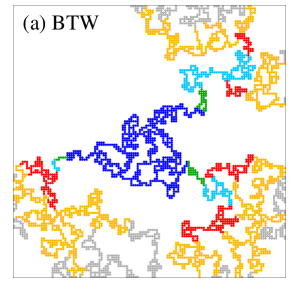
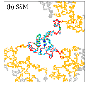
Figure 1: (Colour online) Morphology of a typical avalanche cluster of (a) the BTW and (b) the SSM on percolation backbone generated on an $L=128$ square lattice. Toppling numbers are binned into $5$ equal bins. Different colors correspond to different bins: blue, green, cyan, red, and yellow with decreasing order of toppling numbers. The gray sites are the site of backbone with no toppling. The black border represents the lattice boundary.

The morphology of avalanches in the steady state of both the models are presented here. Typical large avalanches of BTW and SSM obtained in their respective steady states are shown in Fig. 1(a) and 1(b) respectively. These avalanches are obtained on the same percolation backbone generated on a lattice of size $L=128$, dropping sand grain at the central part of the backbone (near to the center of the lattice). The backbone considered here has $3665$ number of lattice sites. For both the cases, the area of the avalanche is $80\%$ of the total number of backbone sites. Maximum toppling for BTW cluster is $154$ whereas that for the SSM is quite high which is $813$. For both the cases, the toppling numbers are binned into $5$ equal sizes. Different colours correspond to the different bin of toppling numbers. Blue colour corresponds to the bin of highest toppling numbers. Green, cyan, red, yellow colours correspond to the bins of the lower and lower toppling numbers respectively. The gray color corresponds to the sites of no toppling. It can be seen that the avalanche in BTW has structured toppling zones, similar to that when the model was studied on the regular lattice [33, 34, *mannaJSP90]. On the other hand, the avalanche of SSM exhibits random mixing of colors representing different toppling numbers as that of an avalanche of SSM on $2$D square lattice [36]. It could also be noted here that though both models preserve the nature of their avalanche morphology, the maximum toppling or the toppling size is quite larger than that of the $2$D regular lattice. This is because the walk dimension is quite high on the backbone than on the regular lattice (which will be discussed in details in terms of avalanche exponents in the following section). Sand grains need more steps to travel to the boundary of the backbone than on a regular lattice starting from the same point. As a result, more toppling occurs in an avalanche on a backbone than on a regular lattice.

5 Multifractal analysis

5.1 Probability distribution function

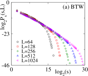
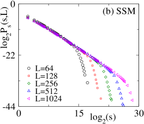
Figure 2: (Colour online) Probability distribution of $s$ for various system sizes $L$ are plotted in (a) for BTW and in (b) for the SSM.

The probability distribution of various avalanche properties $x\in\{s,a,t\}$ are analyzed to characterize the critical steady state of sandpile models. At the steady state, the probability distribution function $P_{x}(x,L)$ of a property $x$ of an avalanche on a percolation backbone generated on a lattice of size $L$ is expected to obey power-law scaling as

$$P_{x}(x,L)=x^{-\tau_{x}}f_{x}(x/L^{D_{x}}),$$ (3)

where $x\in\{s,a,t\}$, $\tau_{x}$ is the corresponding critical exponent, $D_{x}$ is the capacity dimension and $f_{x}$ is the corresponding scaling function. Data for toppling size only are shown in Fig. 2(a) and 2(b) for BTW and SSM respectively for various system size $L$.

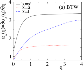
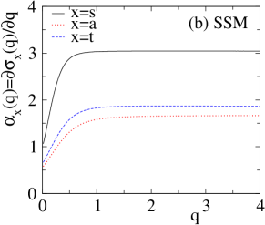
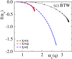
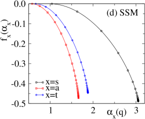
Figure 3: (Colour online) (a) Plot of $\alpha_{x}(q)$ against $q$ for $x=s,a,t$ for (a) the BTW and (b) the SSM. Plot of $\sf f_{x}(\alpha_{x})$ against $\alpha_{x}(q)$ for BTW and SSM in (c) and (d) respectively. Accumulation of points are observed clearly for each $x\in\{s,a,t\}$ in the case of SSM.

To estimate the values of the exponents $\tau_{x}$ and $D_{x}$ defined in Eq. (3), the concept of moment analysis [25, 37] for the various avalanche properties has been employed. The $q$th moment of $x$ is then given by

$$\langle x^{q}\rangle=\int_{0}^{x_{max}}x^{q}P_{x}(x,L)dx\sim L^{\sigma_{x}(q)}$$ (4)

and $\sigma_{x}(q)=[q+1-\tau_{x}]D_{x}$. If the probability distributions obey the scaling form given in Eq.3, the moment scaling function $\sigma_{x}(q)$ would be a piece wise linear : $\sigma_{x}(q)=0$ for $q<\tau_{x}-1$ and $\sigma_{x}(q)=D_{x}[q+1-\tau_{x}]$ for $q>\tau_{x}-1$ for $x\in\{s,a,t\}$. Hence, a multiscaling analysis [23, 24, 38] will be useful in which a spectra of singularity strengths ${\sf f}_{x}(\alpha_{x})$ are obtained. The singularity strengths ${\sf f}_{x}(\alpha_{x})$ can be obtained by Legendre transformation of $\sigma_{x}(q)$ as

$${\sf f}_{x}\left[\alpha_{x}(q)\right]-\sigma_{x}(q)=-q\alpha_{x}(q)$$ (5a)

and

$$\alpha_{x}(q)=\partial\sigma_{x}(q)/\partial q$$ (5b)

which are expected to converge at higher values of $q$. Therefore, a plot of ${\sf f}_{x}(\alpha_{x})$ vs $\alpha_{x}$ should exhibit an accumulation of points for large $q$ in the ${\sf f}_{x}$-$\alpha_{x}$ plane where $\alpha_{x,max}$ and ${\sf f}_{x,min}$ correspond to $D_{x}$ and $-(\tau_{x}-1)D_{x}$ respectively. The analysis not only confirms whether the models exhibit FSS or not but also estimates the exponents in $L\rightarrow\infty$ limit.

Following [38, 39], the technique of direct empirical determination of ${\sf f}_{x}$ has been applied here. Two quantities $\mbox{log}\langle x^{q}(L)\rangle/\mbox{log}L$ and $\langle\mbox{log}(x)x^{q}(L)\rangle/[\mbox{log}(L)\langle x^{q}(L)\rangle]$ have been calculated for finite $L$ and then extrapolated to $L\rightarrow\infty$ limit by a suitable logarithmic correction proposed by Manna [40] to estimate $\sigma_{x}(q)$ and $\alpha_{x}(q)$ for both the models. The values of ${\sf f}_{x}\left[\alpha_{x}(q)\right]$ have been calculated for the moment $q$ in the range $0<q\leq 4$ with $0.01$ interval. For different avalanche properties $x=s,a,t$, the plots of $\alpha_{x}(q)$ against $q$ are shown in Fig. 3(a) for BTW model and in Fig 3(b) for SSM. It can be seen that all the $\alpha_{x}(q)$s do not converge for the BTW model upto $q=4$ whereas in the case of SSM, there is a clear convergence of $\alpha_{x}(q)$, which confirms that though the spatial structure is random fractal the BTW retains its multifractal behavior whereas the SSM obeys FSS. Different spectra of ${\sf f}_{x}(\alpha_{x})$ are plotted in Figs. 3(c) and 3(d) for BTW and SSM respectively. For the case of BTW model, the points are not accumulated at a point on the ${\sf f}-\alpha$ plane which is more prominent for avalanche time $t$. Hence, BTW model exhibits true maultifractal behaviour and no exponent is possible to extract. However, it is recently shown in the $2$D induced model [41], $2$-dimensional cross-section of site dilutated cubic percolatioan lattice, the BTW exponents have similarities with the $2$D Ising universality class [42] and satisfy some hyper-scaling relations. Whereas for SSM, the accumulation of points at large $q$ corresponds to $(\alpha_{x,max},{\sf f}_{x,min})$. The values of $(\alpha_{x,max},{\sf f}_{x,min})$ are found to be ($3.062,-0.472$), ($1.663,-0.479$), and ($1.872,-0.442$) for $x=s,a$, and $t$ respectively and the values of different critical exponents of SSM are then estimated as $\tau_{s}=1.154$, $\tau_{a}=1.288$, $\tau_{t}=1.236$, $D_{s}=3.062$, $D_{a}=1.663$, $D_{t}=1.872$. Note that the values of the exponents obtained for SSM on the backbone are completely different from those known on the square lattice and other deterministic fractals. A detailed comparison of the exponents on the square lattice and deterministic fractal lattices with those on the percolation backbone is given in Table 1. Thus SSM on the percolation backbone obeys FSS but belongs to a new stochastic universality class.

Exponent	Square Lattice	SSTK	Arrowhead	Backbone
	($d=2$)	($d_{f}=1.46$)	($d_{f}=1.58$)	($d_{f}^{B}=1.64$)
$\tau_{s}$	1.273(2)	1.13(2)	1.173(1)	1.154(19)
$\tau_{a}$	1.382(3)	1.273(11)	1.298(1)	1.288(13)
$\tau_{t}$	1.489(9)	1.21(2)	1.279(2)	1.236(14)
$D_{s}$	2.750(6)	2.94(3)	2.793(2)	3.06(2)
$D_{a}$	1.995(3)	1.466(5)	1.584(1)	1.66(1)
$D_{t}$	1.532(8)	1.81(1)	1.673(1)	1.87(1)
$\gamma_{sa}$	1.23(1)	–	–	1.784(4)
$\gamma_{st}$	1.70(1)	–	–	1.547(4)

Table 1: Comparison of different exponents of SSM studied on a regular square lattice, deterministic fractal [semi-inverse square triadic Koch (SSTK) lattice with fractal dimension $1.46$ and arrowhead fractal lattice with fractal dimension $\ln(3)/\ln(2)=1.58$] and on random fractal (percolation backbone) with fractal dimension $1.62$. The values of the exponents for square lattice, SSTK, and Arrowhead are taken from Refs. [43, 30]. The numbers in the parentheses represent the error in the last digit(s) of the value of the exponents. In case of backbone (this work), the errors in $\tau$ estimated from the propagation error in the expression $\tau_{x}=(1-\sf{f}_{x,min}/\alpha_{x,max})$. Similarly the errors in $D$ estimated from the least square fit error during extrapolation.

For lattices with integer dimension it is already known that the average toppling size $\langle s\rangle$ is equivalent to the average number of steps of a random walker on a given lattice before it reaches the boundary starting from an arbitrary lattice point [44, 45]. Thus one could get a relation

$$\sigma_{s}(q=1)=D_{s}(2-\tau_{s})=d_{w},$$ (6)

where $d_{w}$ is the random walk dimension of the lattice considered. This relation for SSM was not only verified for integer dimension [44] but also for various deterministic fractal lattice [29, 30]. In the present case of percolation backbone $\sigma_{s}(q=1)$ for SSM at $L\rightarrow\infty$ is found to be $2.62\pm 0.02$ which is in agreement with the value of $d_{w}\approx 2.64$ estimated by Hong et al. [9] performing exact enumeration of random walks on backbone. Note that taking the measured values of the exponents the quantity $D_{s}(2-\tau_{s})$ has the value $2.59$ which is again within the error bar of the measured value of $\sigma_{s}(1)$. Recently, based on an extensive numerical study Huynh and Pruessner [29, 30] proposed a relation among $D_{s}$, $d_{w}$ and spatial dimension $(d)$ as,

$$D_{s}=ad+bd_{w}$$ (7)

with $a=0.55$ and $b=0.82$. Taking $d=d_{f}^{B}=1.64$ [12], the fractal dimension of the backbone, and $d_{w}=2.64$ [9], the value of $D_{s}$ will be $3.066$ which is again consistent with the measured value. The value of $D_{a}\approx d_{f}^{B}$ is found for both the BTW and SSM as it is expected.

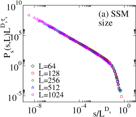
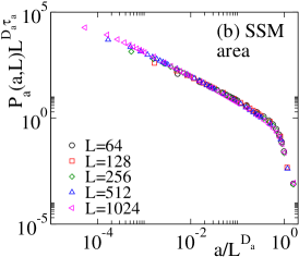
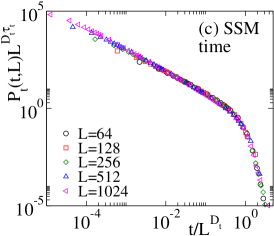
Figure 4: (Colour online) Plot of scaled distribution $P_{x}(x,L)L^{\tau_{x}D_{x}}$ of SSM against scaled variable $x/L^{D_{x}}$ in (a) for $x=s$, (b) for $x=a$, and in (c) for $x=t$. Different curves are for different system sizes $L$. Reasonable collapse of data are observed for all the cases.

To verify the measured values of the exponents and the form of the scaling function defined in Eq. (3) for SSM, a scaled distribution $P_{x}(x,L)L^{\tau_{x}D_{x}}$ is plotted against a scaled variable $x/L^{D_{x}}$ in Fig. 4 for different avalanche properties. For all the cases, the reasonable data collapse confirms the FSS in the SSM defined on the percolation backbone.

5.2 Conditional expectation

The critical behaviour of sandpile models on the backbone is further investigated by studying the conditional expectation values [46] of the avalanche properties through moment analysis technique following Refs. [23, 24]. For a fixed system size $L$, the $q$th moment of the conditional expectation $\langle x^{q}\rangle_{y,L}$ of a property $x$ keeping another property $y$ fixed at a certain value, is defined as [46],

$$\langle x^{q}\rangle_{y,L}=\int_{0}^{\infty}x^{q}P_{x|y,L}(x|y,L)dx$$ (8)

where $P_{x|y,L}(x|y,L)$ is the conditional probability of property $x$ for a fixed value of $y$ and a fixed system size $L$. If $P_{x}(x,L)$ obeys FSS, $P_{x|y,L}(x|y,L)$ can be assumed as $P_{x|y,L}(x|y,L)\sim\delta(x-y^{\gamma_{xy}})$ in the $L\rightarrow\infty$ limit where $\gamma_{xy}$ is a critical exponent. The quantity $\langle x^{q}\rangle_{y,L}$ is then expected to scale with the other property $y$ as

$$\langle x^{q}\rangle_{y,L}\sim y^{\kappa(q)}$$ (9)

where $x\in\{s,a,t\}$ and $\kappa(q)=q\gamma_{xy}$ is a $L$ independent moment exponent. However, for finite system, the quantity $y$ is expected to scale with the system size $L$ as $y\sim L^{\beta_{y}}$ and the conditional moment should be given by

$$\langle x^{q}\rangle_{y,L}\sim L^{\beta_{y}\kappa(q)}$$ (10)

where $\beta_{y}\kappa(q)$ would be the conditional moment scaling function. If the system obeys FSS, the quantity $\beta_{y}\kappa(q)/q$ will be independent of $q$ and would be equal to $\beta_{y}\gamma_{xy}$ [24]. Thus a plot of $\beta_{y}\kappa(q)/q$ versus $\beta_{y}$ will give a unique slope $\gamma_{xy}$ for various values of $q$ and $L$. To measure $\beta_{y}\kappa(q)/q$ the quantity $\log(\langle x^{q}\rangle_{y,L}^{1/q})/\log(L)$ is calculated and plotted against $\beta_{y}=\log(y)/\log(L)$ for $x=s$ and $y=a$ in Fig. 5(a) for BTW and in Fig. 5(b) for the SSM for $q=1,2,3$, and $4$ and for three different system sizes, $L=256$, $512$, and $1024$. It can be seen that the plots for BTW are not parallel to each other. Especially at higher values of $q$, the plots are dispersed and curved which do not allow to measure any critical exponent. Whereas for the case of SSM various plots for different $q$ and $L$ values are parallel to each other for the whole range of $\beta_{a}$ and the measured slope gives the value of $\gamma_{sa}=1.784\pm 0.004$. The values of other conditional critical exponents are also measured following the same method and they are found to be: $\gamma_{st}=1.547\pm 0.004$, $\gamma_{at}=0.873\pm 0.002$. The exponent $\gamma_{xy}$ can also be obtained in terms of the distribution exponents $\tau_{x}$ and $\tau_{y}$ as given in [36]: $\gamma_{xy}=(\tau_{y}-1)/(\tau_{x}-1)$. This scaling relation is satisfied within error bars for $x,y\in{s,a,t}$ for SSM. For example, the values of $\tau_{s}=1.154$ and $\tau_{t}=1.236$ demand that $\gamma_{st}$ should be $1.532$, when the measured value of $\gamma_{st}$ is found to be $1.547\pm 0.004$. Thus, the extended set of exponents obtained here for SSM from moment analysis of both probability distribution and conditional expectation are consistent with the scaling relations. It should be noted here that the exponents $\tau_{x}$ and $\gamma_{xy}$ are found to be different from those obtained for the same model on the regular and other fractal lattices.

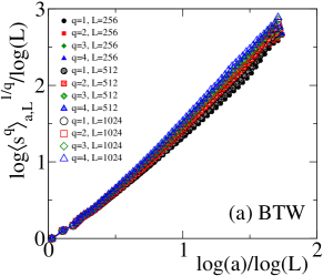
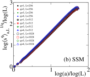
Figure 5: (Colour online) Plot of scaled conditional moment scaling function $\beta_{a}\kappa(q)/q=\log(\langle s^{q}\rangle_{a,L}^{1/q})/\log(L)$, against $\beta_{a}=\log(a)/\log(L)$ for (a) BTW and (b) SSM for three different system sizes $L=256$, $512$, $1024$ and different values of $q$.

6 Time auto-correlation of toppling waves

The multifractal scaling [25] in BTW model on regular lattice is known to be due to the finite auto-corelation in the toppling wave [26, 27, 38]. A toppling wave is the number of topplings during the propagation of an avalanche starting from a critical site without further toppling at the same site and hence each toppling of the critical site creates a new toppling wave [47]. It is then importent to study the time auto-correlation of the toppling waves for the BTW and SSM on the percolation backbone. The time auto-correlation function is defined as

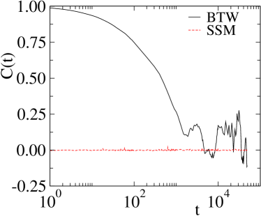
Figure 6: (Color online) Plot of auto-correlation function of toppling waves $C(t)$ against $t$ for BTW model (in solid black line) and for SSM (in red dashed line). For both the models $10^{5}$ toppling waves are considered and they are collected on one realization of the backbone for $L=1024$.

$$C(t)=\frac{\langle s_{k+t}s_{k}\rangle-\langle s_{k}\rangle^{2}}{\langle s_{k}^{2}\rangle-\langle s_{k}\rangle^{2}},$$ (11)

where $t=1,2,\cdots$ and $\langle\cdots\rangle$ represents the time average. $C(t)$ is calculated for both the models — on a system of size $L=1024$, generating $10^{5}$ toppling waves in the steady state. $C(t)$ values obtained are plotted against $t$ in Fig. 6. It can be seen that $C(t)$ in the BTW is positive and hence, the toppling waves are highly correlated, whereas for SSM, the values of $C(t)$ is always $0$ revealing the uncorrelated toppling waves. It should be emphasized here that Karmakar et al. [25] showed that the toppling wave correlation in the BTW-type sandpile model on an regular lattice is essentially due to the precise toppling balance. Thus on the backbone the precise toppling balance is maintained for BTW model and the toppling size which consists of the correlated toppling wave, and the other properties of avalanche like avalanche area and avalanche time do not obey FSS rather than they obey multiscaling behaviour. The uncorrelated toppling wave in SSM leads to the system to obey FSS which is consistence with the observation in the multifractal analysis in previous section.

7 Toppling surface analysis

The analysis of toppling surface of the avalanche, developed in Refs. [48, 49], gives the deeper insight about the topography of the avalanche structure. The values of the toppling number of all the lattice sites of an avalanche define a surface called toppling surface which is obtained for several large avalanches whose area are more than $80\%$ of the total mass of the backbone on which they occur. For a given system size $L$, a total of $N_{\rm span}=4096$ spanning avalanches are taken over $128$ different configurations of backbone. The height of the toppling surface at a position $i$ is given by $S(i)$, the toppling number at $i$th site on the backbone. To study the scaling behaviour of toppling surface a two-point height-height correlation function, the correlation between the toppling numbers of two sites of backbone separated by a certain distance is determined. The expectation value of the square of the difference of toppling numbers $\delta S(r)=\left|S(x+r)-S(x)\right|^{2}$ at two sites separated by a distance $r$ will give the two-point height-height correlation function $C_{L}(r)$. To determine the above said expectation the probability $P[\delta S(r)]$ of a particular value of $\delta S(r)$ occurring for a fixed value of $r$ is estimated for several values of $L$ and $r$. Plots of $P[\delta S(r)]$ versus $\delta S(r)$ for various values of $L$ and $r$ are given in Figs. 7(a) and 7(b) for BTW and SSM respectively. Following Ref. [49], the form of the probability distribution function $P[\delta S(r)]$ is proposed as

$$P[\delta S(r)]=\frac{r^{-2H}}{L^{\zeta}}g\left[\frac{\delta S(r)}{L^{\zeta}r^{2H}}\right]$$ (12)

where $H$ is the Hurst exponent, $\zeta$ is another exponents, and $g$ is the scaling function. Thus for a given $L$, the correlation function $C_{L}(r)$ is obtained as

$$C_{L}(r) = \int_{0}^{\infty}\delta S(r)P[\delta S(r)]d[\delta S_{L}(r)]$$ (13)

$$\sim r^{2H}L^{\zeta}$$

Note that $C_{L}(r)$ is a system size dependent correlation function which is generally observed in stochastic sandpile models [49]. In order to determine the values of the Hurst exponent $H$ and the other exponent $\zeta$, integrated correlation function $I_{L}(R)$ up to a distance $R$ is obtained as

$$I_{L}(R) = \int_{0}^{R}C_{L}(r)dr\sim R^{1+2H}L^{\zeta},$$ (14)

It can be seen that at $R=L$ the value of $I_{L}(R)$ scales as $I_{L}(L)\sim L^{1+2H+\zeta}$. Consequently a plot of $I_{L}(R)/L^{1+2H+\zeta}$ against $R/L$ in log-log scale will give the slope $1+2H$ and from the best collapse of data, one could find the value of $\zeta$. The plots of $\log_{2}[I_{L}(R)/L^{1+2H+\zeta}]$ against $\log_{2}[R/L]$ for various values of $L$ are given in Fig. 7(c) for BTW and in Fig. 7(d) for SSM. Tuning the value of $1+2H+\zeta$ the best collapse is observed when $1+2H+\zeta=4.75\pm 0.03$ for BTW and $1+2H+\zeta=3.87\pm 0.01$ for SSM; while the slope, which is equal to $1+2H$, is measured as $3.00\pm 0.05$ and $1.85\pm 0.02$ for BTW and SSM respectively (given by the straight line in the respective figures). Thus the value of $H$ is found to be $\approx 1$ and $0.425\pm 0.010$ for BTW and SSM, while the value of $\zeta$ is $\approx 1.75$ for BTW and $\approx 2$ for SSM. It should be noted here that the value of the Hurst exponent $H$ ranges from $0$ to $1$ and its value defines the nature of correlation presents in the surface, e.g.; the values $H>1/2$, $H=1/2$, and $H<1/2$ correspond to correlated, uncorrelated and anti-correlated Brownian functions respectively [50]. Since the Hurst exponent of toppling surface of SSM studied on the backbone is $0.42<1/2$, its toppling surfaces are anti-correlated surfaces. On the other hand, the BTW toppling surface is expected to be smooth and less fluctuating as usually seen when the model studied in the two-dimensional square lattice. In-spite of the fact that the substrate (percolation backbone) considered here is random as well as fractal in nature, the toppling surface of the BTW model when studied on such substrate is found to be completely correlated as the Hurst’s exponent is found as $\approx 1$.

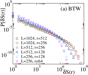
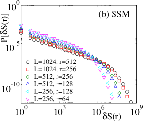
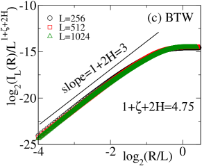
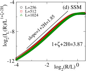
Figure 7: (Colour online) Plot of probability distribution of $\delta S(r)$ for various values of $L$ and $r$ in (a) for BTW and in (b) for SSM. Plot of $I_{L}(R)/L^{1+\zeta+2H}$ against $R/L$ in (c) for BTW and in (d) for SSM for $L=256(\Circle),512(\Box),1024(\triangle)$. The straight line in each figure having slope $1+2H$ is a guide to the eye.

To verify further the values of the exponents the overall surface width $W_{L}$, for a given $L$ is also studied. $W_{L}$ is defined as

$$W_{L}=\left\langle\frac{1}{M_{B}}\sum_{i=0}^{M_{B}}(\bar{S}-S_{i})^{2}\right\rangle^{1/2}$$ (15)

where $M_{B}$ is the mass of the backbone, $\bar{S}$ is the average toppling height, and $\left\langle\cdots\right\rangle$ represents the average over the toppling surfaces. The width $W_{L}$ is expected to scale with $L$ as

$$W_{L}\sim L^{\chi}$$ (16)

where $\chi$ is known as the roughness exponent. To have an estimate of the exponent $\chi$, $W_{L}$ is calculated for different system sizes $L$ and plotted against $L$ in Fig. 8(a) for BTW and Fig. 8(a) for SSM in double logarithmic scale. The best-fitted straight line gives the slope as $\chi_{BTW}=1.74\pm 0.02$ $\chi_{SSM}=1.419\pm 0.016$. To obtain a relationship between the exponents $H$ and $\chi$, the square of the width, $W_{L}^{2}$ can be expressed as

$$W_{L}^{2} = \frac{1}{M_{B}}\int_{0}^{L}C_{L}(r)rdr$$ (17)

Figure 8: (Colour online) Plot of width $W_{L}$ against $L$ in double logarithmic scale for (a) BTW and (b) SSM. The slope of the solid straight line, obtained from the least square fitting, as indicated beside, is the estimated value of $\chi$ for the respective model.

As $M_{B}\sim L^{d_{f}^{B}}$ and the integration is over the plane of the backbone, one could get

$$W_{L}^{2}\sim L^{-d_{f}^{B}+\zeta+d_{f}^{B}+2H}\sim L^{\zeta+2H}$$ (18)

which immediately follows a scaling relation

$$\chi=\zeta/2+H.$$ (19)

This relation is well satisfied within the error bar by the measured exponents. Note that this relation is also satisfied for SSM on $2$D square lattice [49] though the value of $\zeta$ equal to $1$ there. The difference between Hurst exponent and Roughness exponent appeared from system size dependent correlation function as was observed in Ref. [49]. The critical exponent of toppling surfaces and that of the avalanche size capacity dimension can be found to be related as

$$D_{s}=\mbox{spatial dimension}+\chi=d_{f}^{B}+\chi.$$ (20)

For the SSM, taking $d_{f}^{B}=1.64$ and $\chi_{SSM}=0.42$, $D_{s,SSM}$ should be $3.06$ which is in agreement to the measured value of $D_{s,SSM}=3.062$ by the moment analysis of avalanche size. Since the BTW model does not follow FSS, the value of $D_{s,BTW}$ is not well defined and such relation is not satisfied well. However, taking $d_{f}^{B}=1.64$ and the measured value of $\chi_{BTW}=1.74\pm 0.02$, one can obtain $D_{s,BTW}=3.38$ close to the value of $\alpha_{s}(q)$ at higher $q$ (e.g $\alpha_{s}(q=4)$ in Fig. 3(a)).

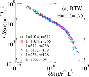
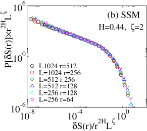
Figure 9: (Colour online) Plot of Scaled distribution $P[\delta S(r)]r^{2H}L$ against scaled variable $\delta S(r)/Lr^{2H}$ for (a) BTW and (b) SSM for various choice of $L$ and $r$. Collapse of data for BTW model is not satisfactory whereas for SSM that is reasonably good.

Finally, to verify the scaling form of the probability distribution $P[\delta S_{L}(r)]$, the value of the exponent $H$ and $\zeta$, a scaled distribution $P[\delta S_{L}(r)]r^{2H}L$ against a scaled variable $\delta S_{L}(r)/Lr^{2H}$ for different values $L$ and $r$ are plotted in Figs. 9(c) and (d). Taking respective values of $H$ and $\zeta$ of a given model, an attempt has been made to collapse the data. It can be seen that while a good data collapse is observed for SSM taking $H=0.42$ and $\zeta=2$, for BTW the collapsed data is not satisfactory which could be due to the fact that BTW model does not obey FSS ansatz. On the other hand, reasonable data collapse for the SSM not only confirms the proposed scaling function given in Eq. (12) is correct but also verify the measured correct exponents.

8 Conclusion

Both the deterministic and the stochastic sandpile models have been carried out on the percolation backbone in order to verify the effect of a random fractal on the critical properties of such sandpile models. By extensive numerical analysis, an extended set of critical exponents of both the models has been estimated and verified through various scaling analysis. Multifractal analysis of the probability distribution functions and the expectations of the avalanche properties suggest that though the spatial structure is a random fractal, the BTW model preserves its multiscaling behaviour due to its complete toppling balance, whereas the SSM retains its robust finite size scaling behaviour. Moreover, the toppling surface analysis has been carried out and the attempt has been made to explore the effect of the fractal dimension of the backbone on the characteristics of the toppling surface for both the models. New scaling relations have been developed in terms of fractal dimension of the backbone and such scaling relations are verified numerically. As the critical exponents depend on the dimension of the underlying structures, the values of the critical exponents of SSM on the percolation backbone are found to be very different from those for the model defined on the regular and other fractal lattices. Hence, SSM on the percolation backbone belongs to a new stochastic universality class.

Acknowledgments: This work is partially supported by DST, Government of India through project No. SR/S2/CMP-61/2008. Availability of computational facility, “Newton HPC” under DST-FIST project (No. SR/FST/PSII-020/2009) Government of India, of Department of Physics, IIT Guwahati is gratefully acknowledged.

References

- [1] B. B. Mandelbrot, Fractals: Form, chance, and dimension, W. H. Freedman and Co., New York, 1977
- [2] D. Dhar, Journal of Mathematical Physics 18, 577 (1977)
- [3] Y. Gefen, B. B. Mandelbrot, and A. Aharony, Phys. Rev. Lett. 45, 855 (1980)
- [4] J. M. Carmona, U. M. B. Marconi, J. J. Ruiz-Lorenzo, and A. Tarancón, Phys. Rev. B 58, 14387 (1998)
- [5] G. Pruessner, D. Loison, and K. D. Schotte, Phys. Rev. B 64, 134414 (2001)
- [6] A. L. Windus and H. J. Jensen, Physica A: Statistical Mechanics and its Applications 388, 3107 (2009)
- [7] D. Stauffer and A. Aharony, Introduction to Percolation Theory, Taylor and Francis, London, 1994
- [8] A. Bunde and S. Havlin, Fractals and Disordered Systems, Springer-Verlag, Berlin, 1991
- [9] D. C. Hong, S. Havlin, H. J. Herrmann, and H. E. Stanley, Phys. Rev. B 30, 4083 (1984)
- [10] P. Grassberger, Physica A: Statistical Mechanics and its Applications 262, 251 (1999)
- [11] M. Barthélémy, S. Buldyrev, S. Havlin, and H. Stanley, Phys. Rev. E 60, R1123 (1999)
- [12] M. Porto, A. Bunde, S. Havlin, and H. Roman, Phys. Rev. E 56, 1667 (1997)
- [13] R. Rammal and G. Toulouse, Journal de Physique Lettres 44, 13 (1983)
- [14] M. Grova and A. Hansen, Journal of Physics: Conference Series 319, 012009 (2011)
- [15] M. Najafi and M. Ghaedi, Physica A: Statistical Mechanics and its Applications 427, 82 (2015)
- [16] S. B. Lee and J. S. Kim, Phys. Rev. E 87, 032117 (2013)
- [17] P. Bak, How Nature Works: The Science of Self-Organized Criticality, Copernicus, New York, 1996
- [18] H. J. Jensen, Self-Organized Criticality, Cambridge University Press, Cambridge, 1998
- [19] P. Bak, C. Tang, and K. Wiesenfeld, Phys. Rev. Lett. 59, 381 (1987)
- [20] P. Bak, C. Tang, and K. Wiesenfeld, Phys. Rev. A 38, 364 (1988)
- [21] D. Dhar, Physica A 263, 4 (1999), and references therein
- [22] D. Dhar, Physica A 369, 29 (2006)
- [23] M. DeMenech, A. L. Stella, and C. Tebaldi, Phys. Rev. E 58, R2677 (1998)
- [24] C. Tebaldi, M. DeMenech, and A. L. Stella, Phys. Rev. Lett. 83, 3952 (1999)
- [25] R. Karmakar, S. S. Manna, and A. L. Stella, Phys. Rev. Lett. 94, 088002 (2005)
- [26] M. DeMenech and A. L. Stella, Phys. Rev. E 62, R4528 (2000)
- [27] M. DeMenech and A. L. Stella, Physica A 309, 289 (2002)
- [28] H. Huynh, G. Pruessner, and L. Chew, J. Stat. Mech 2011, P09024 (2011)
- [29] H. N. Huynh, L. Y. Chew, and G. Pruessner, Phys. Rev. E 82, 042103 (2010)
- [30] H. N. Huynh and G. Pruessner, Phys. Rev. E 85, 061133 (2012)
- [31] J. Hoshen and R. Kopelman, Phys. Rev. B 14, 3438 (1976)
- [32] W.-G. Yin and R. Tao, Physica B: Condensed Matter 279, 84 (2000)
- [33] K. Christensen and Z. Olami, Phys. Rev. E 48, 3361 (1993)
- [34] P. Grassberger and S. S. Manna, J. Phys (France) 51, 1077 (1990)
- [35] S. S. Manna, J. Stat. Phys. 59, 509 (1990)
- [36] S. B. Santra, S. R. Chanu, and D. Deb, Phys. Rev. E 75, 041122 (2007)
- [37] S. Lübeck, Phys. Rev. E 61, 204 (2000)
- [38] A. L. Stella and M. DeMenech, Physica A 295, 101 (2001)
- [39] A. Chhabra and R. V. Jensen, Phys. Rev. Lett. 62, 1327 (1989)
- [40] S. S. Manna, Physica A 179, 249 (1991)
- [41] M. N. Najafi and H. Dashti-Naserabadi, Journal of Statistical Mechanics: Theory and Experiment 2018, 023211 (2018)
- [42] M. N. Najafi, Journal of Statistical Mechanics: Theory and Experiment 2015, P05009 (2015)
- [43] A. Ben-Hur and O. Biham, Phys. Rev. E 53, R1317 (1996)
- [44] H. Nakanishi and K. Sneppen, Phys. Rev. E 55, 4012 (1997)
- [45] Y. Shilo and O. Biham, Phys. Rev. E 67, 066102 (2003)
- [46] K. Christensen, H. C. Fogedby, and H. J. Jensen, J. Stat. Phys. 63, 653 (1991)
- [47] V. B. Priezzhev, D. V. Ktitarev, and E. V. Ivashkevich, Phys. Rev. Lett. 76, 2093 (1996)
- [48] J. A. Ahmed and S. B. Santra, Europhys. Lett. 90, 50006 (2010)
- [49] H. Bhaumik, J. A. Ahmed, and S. B. Santra, Phys. Rev. E 90, 062136 (2014)
- [50] P. Mealin, Fractals, scaling and growth far from equilibrium, Cambridge University Press, Cambridge, 1998