KMT-2018-BLG-1292: A Super-Jovian Microlens Planet in the Galactic Plane

Abstract

We report the discovery of KMT-2018-BLG-1292Lb, a super-Jovian $M_{\rm planet}=4.5\pm 1.3\,M_{J}$ planet orbiting an F or G dwarf $M_{\rm host}=1.5\pm 0.4\,M_{\odot}$, which lies physically within ${\cal O}(10\,{\rm pc})$ of the Galactic plane. The source star is a heavily extincted $A_{I}\sim 5.2$ luminous giant that has the lowest Galactic latitude, $b=-0.28^{\circ}$, of any planetary microlensing event. The relatively blue blended light is almost certainly either the host or its binary companion, with the first explanation being substantially more likely. This blend dominates the light at $I$ band and completely dominates at $R$ and $V$ bands. Hence, the lens system can be probed by follow-up observations immediately, i.e., long before the lens system and the source separate due to their relative proper motion. The system is well characterized despite the low cadence $\Gamma=0.15$–$0.20\,{\rm hr^{-1}}$ of observations and short viewing windows near the end of the bulge season. This suggests that optical microlensing planet searches can be extended to the Galactic plane at relatively modest cost.

1 Introduction

As a rule, optical microlensing searches heavily disfavor regions of high extinction and, as a result, systematically avoid the Galactic plane. For example, prior to the start of OGLE-IV (the fourth phase of the Optical Gravitational Lensing Experiment, Udalski et al. 2015a) in 2010, all but a small fraction of Galactic-bulge microlensing observations were restricted to the southern bulge despite the fact that the stellar content of the lines of sight toward the northern and southern bulge are extremely similar. With its larger format camera, OGLE-IV began systematically covering the northern bulge, but mainly at very low cadence. Hence, it remained the case that the great majority of observations were toward the southern bulge.

However, Poleski (2016) showed that the microlensing event rate is basically proportional to the product of the surface density of clump stars and the surface density of stars below some magnitude limit (in the principal survey band), e.g., $I<20$; the two numbers being proxies for the column densities of lenses and sources, respectively. Guided in part by this work, the Korea Microlensing Telescope Network (KMTNet, Kim et al. 2016) devised an observing strategy that much more heavily favored the northern bulge, which accounts for about 37% of the area covered and 24% of all the observations. Nevertheless, even with this more flexible attitude toward high-extinction fields, KMTNet still followed previous practice in systematically avoiding the Galactic plane. See Figure 12 of Kim et al. (2018a).

Indeed, there is an additional reason for avoiding fields with high or very high extinction. That is, even if the high stellar-lens column densities near the plane partially compensate for the lower column density of sources, it remains the case that events, particularly planetary and binary events, in very high extinction fields are more difficult to interpret. Very often these events have caustic crossings from which one can usually measure $\rho=\theta_{*}/\theta_{\rm E}$, i.e., the ratio of the angular radius of the source to the Einstein radius. Then, one can usually determine $\theta_{*}$ from the offset of the source relative to the red clump in color and magnitude (Yoo et al., 2004). However, the color measurement required for this technique is only possible if the event is detected in a second band, which is usually $V$ band in most microlensing surveys. But $V$-band observations rarely yield usable results in very high-extinction fields. Hence, one must either take special measures to observe the event in a redder band (e.g., $H$) or one must estimate $\theta_{*}$ without benefit of a color measurement, which inevitably substantially increases the error in $\theta_{*}$ (and so $\theta_{\rm E}=\theta_{*}/\rho$).

As a result of the almost complete absence of optical microlensing observations toward the Galactic plane, there is essentially no experience with how these theoretical concerns translate into practical difficulties, and similarly no practical approaches to overcoming these difficulties. This is unfortunate because the Galactic plane could potentially provide important complementary information to more standard fields in terms of understanding the microlensing event rate and Galactic distribution of planets.

While this shortcoming is widely recognized, the main orientation of researchers in the field has been to await infrared microlensing surveys. Gould (1995) advocated a “K-band microlensing [survey] of the inner galaxy”. Although his focus was on regions projected close to the Galactic center, the same approach could be applied to any high-extinction region, in particular the Galactic plane. In fact, PRIME, a 1.8m field telescope with 1.3 deg² camera to be installed at SAAO in South Africa, will be the first to conduct a completely dedicated IR microlensing survey (T. Sumi 2019, private communication), While the exact survey strategy has not yet been decided, PRIME will certainly focus on heavily extincted regions toward the inner Galaxy. The VISTA Variables in the Via Lactea (VVV; Minniti et al. 2010; Saito et al. 2012) Microlensing Survey (Navarro et al., 2017, 2018) has already conducted wide-field IR observations covering a $(20.4^{\circ}\times 1.1^{\circ})$ rectangle of the Galactic plane spanning 2010-2015. They discovered 630 microlensing events. However, given their low cadence (ranging from 73 to 104 epochs over 6 years), they were not sensitive to planetary deviations. In addition, Navarro et al. (2019) used VVV near-IR photometry to search for microlensing events in fields along the Galactic minor axis, ranging from $b=-3.7$ to $b=4$, covering a total area of $\sim 11.5\,{\rm deg}^{2}$. They found $N=238$ new microlensing events in total, $N=74$ of which have bulge red clump (RC) giant sources. They found a strong increase of the number of microlensing events with Galactic latitude toward the plane, both in the total number of events and in the RC subsample, in particular, an order of magnitude more events at $b=0$ than at $|b|=2$ along the Galactic minor axis. This gradient is much steeper than predicted by models that had in principle been tuned to explain the observations from the optical surveys farther from the plane.

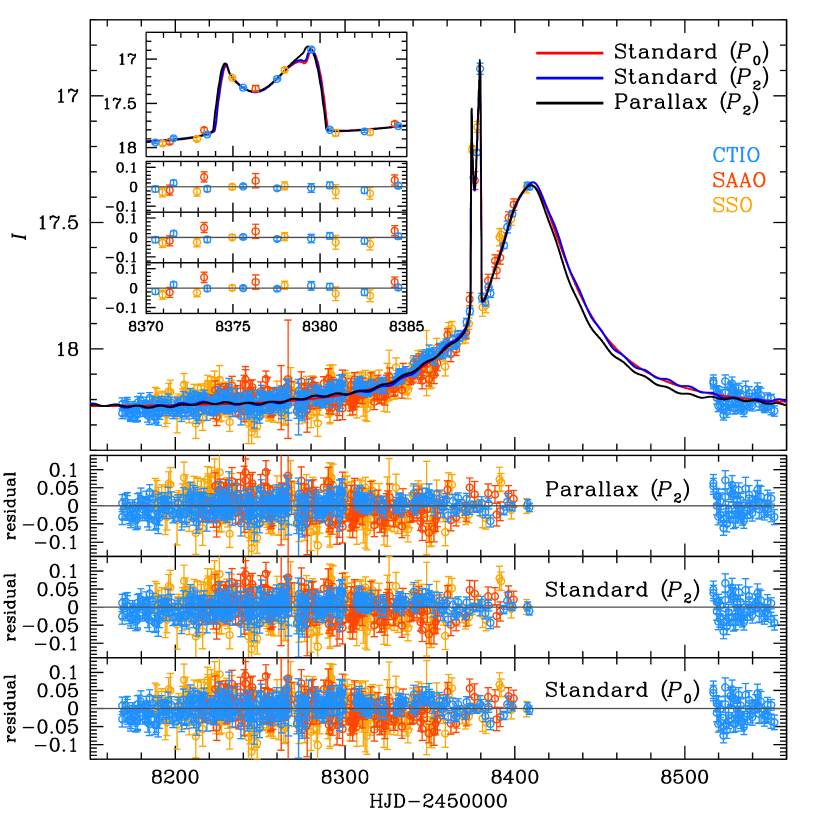
Figure 1: KMT data and best-fit model for KMT-2018-BLG-1292. The lower three panels show the residuals from the final parallax model, a standard model that includes two periodic wave forms, and a standard model without additional wave forms, respectively. The inset shows a zoom of the caustic region. Note that although the source spent six days transiting the caustic, there are only six data points from all three KMT observatories combined. This is partly because the event lies in a low-cadence field and partly because the anomaly occurred very near the end of the season, when the bulge is visible for only a few hours per night.

Shvartzvald et al. (2017) conducted a survey of high-extinction microlensing fields (Figure 1 of Shvartzvald et al. 2017 and Figure 1 of Shvartzvald et al. 2018), which had substantially higher cadence despite the relatively short viewing window from the 3.8m UKIRT telescope in Hawaii. This yielded the first infrared detection of a microlensing planet, UKIRT-2017-BLG-001Lb, which lies projected just $0.33^{\circ}$ from the Galactic plane and $0.35^{\circ}$ from the Galactic center (Shvartzvald et al., 2018). Both values were by far the smallest for any microlensing planet up to that point. They estimated the extinction at $A_{K}=1.68$, which corresponds approximately to $A_{I}\simeq 7A_{K}=11.8$.

This high extinction value might lead one to think that such planets are beyond the reach of optical surveys. In fact, KMTNet routinely monitors substantial areas of very high extinction simply because its cameras are so large that these are “inadvertently” covered while observing neighboring regions of lower extinction and high stellar density. For example, KMT-2018-BLG-0073 lies at $(l,b)=(+2.32,+0.27)$ and has $A_{K}=1.3$. This raises the possibility that optical surveys could in fact probe very high extinction regions as well, albeit restricted to monitoring exceptionally luminous sources or very highly magnified events.

Here we report the discovery of the planet KMT-2018-BLG-1292Lb, which at Galactic coordinates $(l,b)=(-5.23,-0.28)$ is the closest to the Galactic plane of any microlensing planet to date. The planetary perturbation is well characterized despite the fact that it occurred near the end of the season when it could be observed only about three hours per night from each site and that it lies in KMTNet’s lowest cadence field. Thus, this detection in the face of these moderately adverse conditions suggests that optical surveys could contribute to the study of Galactic-plane planetary microlensing at relatively modest cost.

2 Observations

KMT-2018-BLG-1292 is at (RA,Dec) = (17:33:42.62,$-33$:31:14.41) corresponding to $(l,b)=(-5.23,-0.28)$. It was discovered by applying the KMTNet event-finder algorithm (Kim et al., 2018a) to the full-season of 2018 KMTNet data, which were taken from three identical 1.6m telescopes equipped with $(2^{\circ}\times 2^{\circ})$ cameras in Chile (KMTC), South Africa (KMTS), and Australia (KMTA). The event lies in KMT field BLG13, which was observed in the $I$ band at cadences of $\Gamma=0.2\,{\rm hr}^{-1}$ from KMTC and $\Gamma=0.15\,{\rm hr}^{-1}$ from KMTS and KMTA. One out of every ten $I$-band observations was matched by an observation in the $V$ band. However, the $V$-band light curve is not useful due to high extinction.

The event was initially classified as “clear microlensing” based on the relatively rough DIA pipeline photometry (Alard & Lupton, 1998; Woźniak, 2000), but planetary features were not obvious. The possibly planetary anomaly was noted on 5 January 2019, when the data were routinely re-reduced using the KMTNet pySIS (Albrow et al., 2009) pipeline as part of the event-verification process. The first modeling was carried almost immediately, on 8 January 2019. This confirmed the planetary nature, thus triggering final tender-loving care (TLC) reductions. But, in addition, it also made clear that the event might still be ongoing after the bulge had passed behind the Sun.

This led KMTNet to take two measures to obtain additional data. First, KMTNet began observing BLG13 from KMTC on 2 February, which was 17 days before the start of its general bulge observations. This was made possible by the fact that KMT-2018-BLG-1292 lies near the western edge of the bulge fields and so can be observed earlier in the season than most fields, given the pointing restrictions due to the telescope design. Second, KMTNet contacted C. Kochanek for special permission to obtain nine epochs of observations (17 pointings) from 31 January 2019 to 8 February 2019 on the dual channel (optical/infrared) ANDICAM camera (DePoy et al., 2003) on the 1.3m SMARTS telescope in Chile. The primary objective of these observations was to obtain $H$-band data, which could yield an $I-H$ color, provided that the event remained magnified at these late dates. As mentioned above, it was already realized that the KMT $V$-band data would not yield useful source-color information.

However, because the source turned out to be a low-amplitude variable (see Section 3.1) while the magnification at the first ANDICAM $H$-band observation was low, $A\sim 1.1$, the $(I-H)$ color measurement from these data was significantly impacted by systematic uncertainties. Fortunately, the VVVX survey (Minniti, 2018) obtained seven $K_{s}$-band data points on the rising part of the light curve, including three with magnifications $A=1.47$–1.58. While these are, of course, also affected by systematics from source variability, the impact is a factor $\sim 5$ times smaller. Hence, in the end, we use these VVV survey data to measure the source color.

3 Light Curve Analysis

3.1 Source and Baseline Variability

The light curve exhibits low-level (few percent) variability, including roughly periodic variations with period $P\sim 13\,$days. This level of variation is far too small to have important implications for deriving basic model parameters, but could in principle affect subtle higher-order effects, in particular the microlens parallax. For clarity of exposition, we therefore initially ignore this variability when exploring static models (Section 3.2), and then use these to frame the investigation of the variability. We then account for its impact on the microlensing parameters (and their uncertainties) after introducing higher-order effects into the modeling in Section 3.3.

3.2 Static Model

Figure 1 shows the KMT data and best-fit model for KMT-2018-BLG-1292. With the exception of a strong anomaly lasting $\delta t\simeq 6\,$days, the 2018 data take the form of the rising half of a standard Paczyński (1986) single-lens single-source (1L1S) curve. The early initiation of 2019 observations, discussed in Section 2, then capture the extreme falling wing of the same Paczyński profile.

We therefore begin by searching for static binary (2L1S) models, which are characterized by seven non-linear parameters: $(t_{0},u_{0},t_{\rm E},q,s,\alpha,\rho)$. The first three are the standard 1L1S Paczyński parameters, i.e., the time of lens-source closest approach, the impact parameter (in units of the Einstein radius $\theta_{\rm E}$), and the Einstein radius crossing time. The next three characterize the planet, i.e., the planet-host mass ratio, the magnitude of the planet-host separation (in units of $\theta_{\rm E}$), and the orientation of this separation relative to the lens-source relative proper-motion ${\mbox{\boldmath$\mu$}}_{\rm rel}$. The last, $\rho\equiv\theta_{*}/\theta_{\rm E}$, is the normalized source radius.

We first conduct a grid search over $(s,q)$, in which these two parameters are held fixed while all others are allowed to vary in a Markov chain Monte Carlo (MCMC). The Paczyński parameters are seeded at values derived from a 1L1S fit (with the anomaly removed), and $\alpha$ is seeded at six values drawn uniformly around the unit circle. Given the very high extinction toward this field $A_{I}\simeq 7A_{K}=5.2$ and the relatively bright baseline flux $I_{\rm base}\sim 18.2$, the source is very likely to be a giant. In view of this, we seed the normalized source radius at $\rho=0.005$. This procedure yields only one local minimum. We then allow all seven parameters to vary and obtain the result shown as the first model in Table 1.

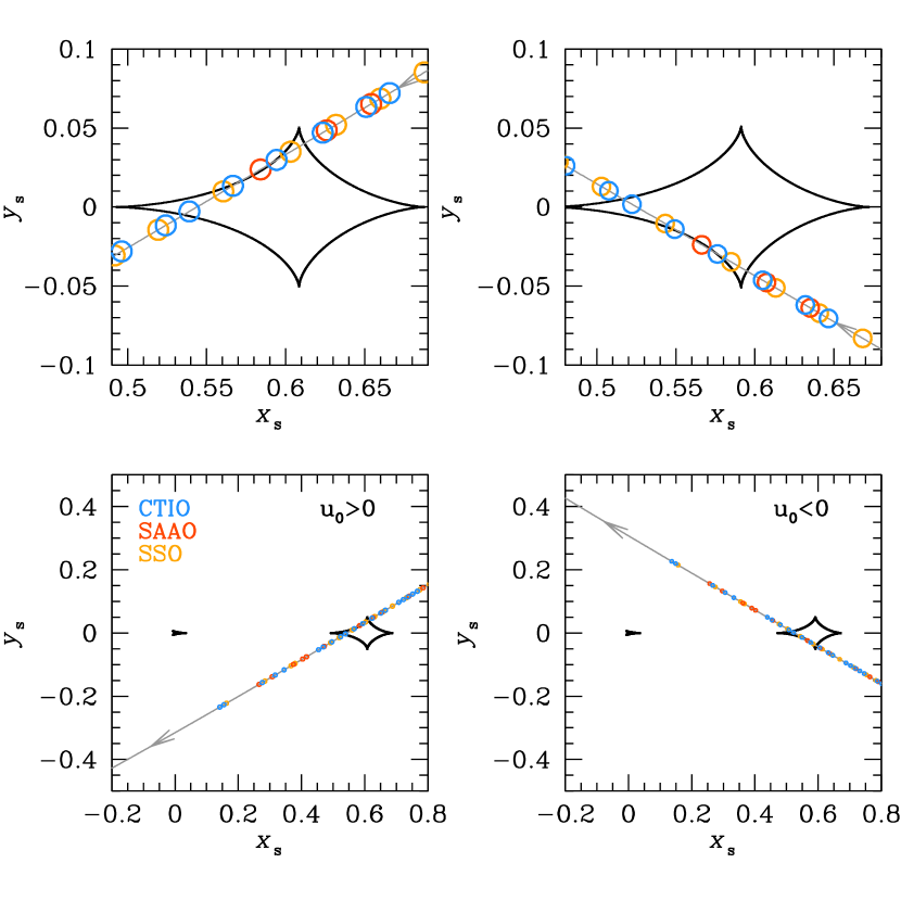
Figure 2: Geometry for the two parallax models ($u_{0}>0$ and $u_{0}<0$) of KMT-2018-BLG-1292. The closed contours show the planetary caustic. The upper panels are zooms of the regions surrounding these caustics. The source size is shown to scale at the epochs of observation, which are color-coded by observatory. Note that the source travels along the edge of the caustic, so that all six data points (spread out over six days) are affected by the caustic, which enables a reasonably good measurement of the normalized source size $\rho=\theta_{*}/\theta_{\rm E}$. While this close alignment of the source trajectory with the edge of the caustic is unusual, the large value of $\rho$ (due to the very large source) implies that random trajectories through the caustic would likely intersect or closely approach the caustic contour several times.

The only somewhat surprising element of this analysis is that $\rho$ is measured reasonably well, with $\sim 15\%$ precision. This is unexpected because one does not necessarily expect to measure $\rho$ with such sparse sampling, roughly one point per day. However, from the solution, the source-radius crossing time is $t_{*}\equiv\rho t_{\rm E}=9.4\,$hrs, so that the diameter crossing time is almost one day. Moreover, as shown by the caustic geometry in Figure 2, the source actually runs almost tangent to caustic, which means that all six data points are affected by the caustic (and so finite-source effects). Hence, the relatively good measurement of $\rho$ is partly due to a generic characteristic of giant-star sources (which in turn are much more likely for optical microlensing searches in extincted fields) and partly due to a chance alignment of the source trajectory with the caustic. We note that UKIRT-2017-BLG-001 (Shvartzvald et al., 2018) had a similarly good ($\sim 10\%$) $\rho$ measurement with similar O(1 day) cadence, and for similar reasons: large source, whose detection was favored by heavy extinction, and consequently long $t_{*}$ ($\sim 16\,$ hrs).

3.3 Parallax Models

We next attempt to measure the microlens parallax vector (Gould, 1992, 2000),

$${\mbox{\boldmath$\pi$}}_{\rm E}\equiv{\pi_{\rm rel}\over\theta_{\rm E}}{{\mbox{\boldmath$\mu$}}_{\rm rel}\over\mu_{\rm rel}},\qquad\theta_{\rm E}^{2}\equiv\kappa M\pi_{\rm rel},\qquad\kappa\equiv{4G\over c^{2}{\rm AU}}\simeq 8.1\,{{\rm mas}\over M_{\odot}}.$$ (1)

where, $M$ is the lens mass, ${\mbox{\boldmath$\mu$}}_{\rm rel}$ is the instantaneous geocentric lens-source relative proper motion, and $\pi_{\rm rel}$ is the lens-source relative parallax. Because the parallax effect due to Earth’s annual motion is quite subtle, such a measurement can be affected by source variability. Hence we must simultaneously model this variability together with the microlens parallax in order to assess its impact on both the best estimate and uncertainty of ${\mbox{\boldmath$\pi$}}_{\rm E}$.

3.3.1 Significant Parallax Constraints Are Expected

The relatively long timescale, $t_{\rm E}\simeq 67\,$days, of the standard solution in Table 1 suggests that it may be possible to measure or strongly constrain ${\mbox{\boldmath$\pi$}}_{\rm E}$. In addition to the relatively long timescale, the presence of sharply defined peaks (from the anomaly) tend to improve microlens parallax measurements (An & Gould, 2001). Finally, while it would be relatively difficult to measure ${\mbox{\boldmath$\pi$}}_{\rm E}$ from 2018 data alone (because these contain only the rising part of the light curve), the 2019 data on the extreme falling wing add significant constraints to this measurement. We therefore add two parameters to the modeling $(\pi_{{\rm E},N},\pi_{{\rm E},E})$, i.e., the components of ${\mbox{\boldmath$\pi$}}_{\rm E}$ in equatorial coordinates.

Because parallax effects, which are due to Earth’s orbital motion, can be mimicked in part by orbital motion of the lens system (Batista et al., 2011; Skowron et al., 2011), one should always include lens motion, at least initially, when incorporating parallax into the fit. We model this with two parameters, ${\mbox{\boldmath$\gamma$}}\equiv((ds/dt)/s,d\alpha/dt)$, where $ds/dt$ is the instantaneous rate of change in separation and $d\alpha/dt$ is the instantaneous rate of change of the orientation of the binary axis. Note that all “instantaneous” quantities $({\mbox{\boldmath$\mu$}},{\mbox{\boldmath$\gamma$}})$ are defined at time $t=t_{0}$. However, we find that these two additional parameters are not significantly correlated with the parallax and are also not significantly constrained by the fit. Hence, we remove them from the fit.

3.3.2 Accounting for Variability

As mentioned in Section 3.1, the source shows low-level variations in the standard-model residuals. We will show in Section 4 that the source is a luminous red giant, so source variability would not be unexpected. These variations do not significantly affect the static model (and so were ignored up to this point) but could affect the parallax measurement, which depends on fairly subtle distortions of the light curve relative to the one defined by a static geometry. We therefore simultaneously fit for this variability together with the nine other non-linear parameters describing the 2L1S parallax solution. This will allow us, in particular, to determine whether the parallax parameters $(\pi_{{\rm E},N},\pi_{{\rm E},E})$ are correlated with the variability parameters. We consider models that incorporate variability into an “effective magnification”

$$A_{\rm eff}(t)=A(t;t_{0},u_{0},t_{\rm E},q,s,\alpha,\rho,\pi_{{\rm E},N},\pi_{{\rm E},E})\biggl{[}1+\sum_{i=1}^{N_{\rm per}}a_{i}\sin\biggl{(}{2\pi t\over P_{i}}+\phi_{i}\biggr{)}\biggr{]},$$ (2)

where $(a_{i},P_{i},\phi_{i})$ are the amplitude, period, and phase of each of the $N_{\rm per}$ wave forms that are included.

We search for initial values of the wave-form parameters by first applying Equation (2) to static models with the microlensing parameters seeded at the best fit non-variation model. We set $N_{\rm per}=1$ and find the three wave-form parameters. We then set $N_{\rm per}=2$ and seed the previous $(7+3)=10$ non-linear parameters at the $N_{\rm per}=1$ solution in order to find the next three. In principle this procedure could be repeated, but we find no additional significant periodic variations.

We seeded the first component with $P_{1}=11\,$days based on our by-eye estimate of the periodic variations. Somewhat surprisingly, this fit converged to $P_{1}\sim 70\,$days. Hence, we seeded the second component again with $P_{2}=11\,$days, which converged to $P_{2}\simeq 13\,$days. We show this $N_{\rm per}=2$ standard model in Table 1 next to the model without periodic variation. As anticipated in Section 3.2, the introduction of periodic components has virtually no effect on the standard microlensing parameter estimates, although the fit is improved by $\Delta\chi^{2}=27$ for six degrees of freedom (dof).

These values served as benchmarks for the next phase of simultaneously fitting for parallax and periodic variations, in which the parallax fits could in principle become coupled to long-term variations. We seed the $N_{\rm per}=1$ parallax fits with a variety of periods, but these always converge to $P_{1}\sim 63\,$days. We then seed $P_{2}=13\,$days, which then converges to a similar value. Adding more wave forms does not significantly improve the fit.

3.3.3 Parallax Model Results

Table 1 shows the final results, i.e., for nine microlensing parameters plus six periodic-variation parameters. As usual, we test for the “ecliptic degeneracy”, which approximately takes $(u_{0},\alpha,\pi_{{\rm E},N})\rightarrow-(u_{0},\alpha,\pi_{{\rm E},N})$ (Skowron et al., 2011) and present this solution as well in Table 1.

In addition, in Table 2, we show the evolution of key microlens parameters as additional period terms are introduced. In fact, neither the microlens parallax nor the other key microlens parameters change significantly as a result of incorporating periodic variability into the fits.

Because both $\pi_{\rm E}$ and $\rho$ are measured, one can infer the lens mass and lens-source relative parallax via,

$$M={\theta_{\rm E}\over\kappa\pi_{\rm E}},\qquad\pi_{\rm rel}=\theta_{\rm E}\pi_{\rm E},$$ (3)

provided that the angular source size $\theta_{*}$ (and so $\theta_{\rm E}=\theta_{*}/\rho$) can be determined from the color-magnitude diagram (CMD).

4 Color-Magnitude Diagram

There are two challenges to applying the standard procedure (Yoo et al., 2004) of putting the source star on an instrumental CMD in order to determine $\theta_{*}$. Both challenges derive from the fact that the event lies very close to the Galactic plane. First, the extinction is high, which implies that the $V$-band data, which are routinely taken, will not yield an accurate source color. Fortunately, there are $K_{s}$ data from the VVVX survey taken when the event was sufficiently magnified to measure the $K_{s}$ source flux.

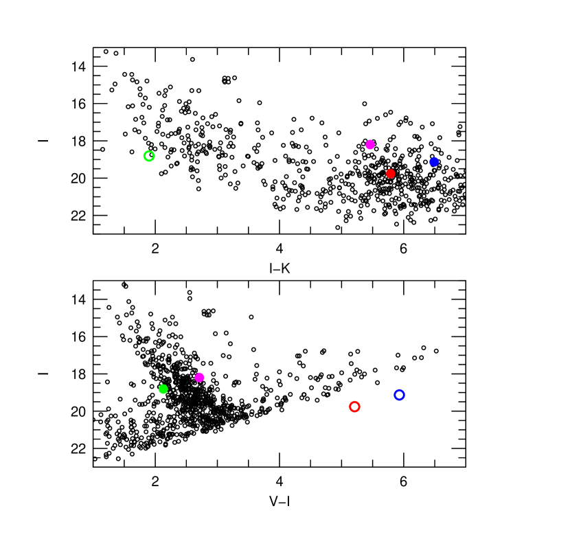
Figure 3: Color-magnitude diagrams (CMDs) in $I$ vs. $(I-K)$ (upper) and $I$ vs. $(V-I)$ (lower). The black points are field stars from a $(2^{\prime}\times 2^{\prime})$ square centered on KMT-2018-BLG-1292. The large circles are the positions of the source (blue), blend (green), “baseline object” (magenta) and clump centroid (red). The filled circles are measured, while the open circles are estimated (and shown for illustration only). The source (blue) is a luminous and very red giant. The blend (green) is a foreground main-sequence star, lying in front of the majority of the dust column toward the Galactic bar.

The second issue is more fundamental. The upper panel in Figure 3 shows an $I$ versus $(I-K)$ CMD, where the $I$-band data come from pyDIA reductions of the field stars within a $2^{\prime}\times 2^{\prime}$ square centered on the event and the $K$-band data come from the VVV catalog. The position of the “baseline object” (magenta) is derived from the field-star photometry of these two surveys, while the position of the source star (blue) is derived from the $f_{S}$ measurements from the model fit to the light curves. The position of the blended light is shown as an open circle because, while its $I$-band magnitude is measured from the fit, its $K$-band flux is too small to be reliably determined. Hence its position is estimated from the $I$ versus $(V-I)$ CMD, which is described immediately below. The centroid of the red clump is shown in red.

The lower panel of Figure 3 shows the same quantities for the $I$ versus $(V-I)$ CMD. It is included to facilitate analysis of the properties of the blend, which is discussed further below. In this case, the source (blue) and clump centroid (red) are shown as open symbols because neither can be reliably determined from the data and so are estimates rather then measurements.

The source lies $\Delta(I-K,I)=(+0.70,-0.63)$ redward and brighter than the clump. We first interpret this position under the assumption that the lens suffers similar extinction as the clump itself. In this case, the source is a very red, luminous giant, $[(I-K)_{0},M_{I}]\simeq(2.1,-0.7)$, which would explain why it is a low-amplitude semi-regular variable.

Adopting the assumption that the source suffers the same extinction as the clump, together with the intrinsic clump position $[(V-I),I]_{0,\rm cl}=(1.06,14.66)$ from Bensby et al. (2013) and Nataf et al. (2013), as well as the color-color relations of Bessell & Brett (1988), we obtain $[(V-K),K]_{0}=(3.90,11.87)$. Then using the color/surface-brightness relation of Groenewegen (2004)

$$\log(\theta_{*}/\mu{\rm as})=3.286-0.2\,K_{0}+0.039(V-K)_{0},$$ (4)

we obtain

$$\theta_{*}=11.59\pm 1.00\,\mu{\rm as}.$$ (5)

The error bar in Equation (5) is determined as follows. First, while the formal error $\Delta(I-K)$ (from fitting the $I$ and $K$ light curves to the model and centroiding the clump) is only $\sim 0.05\,$mag, we assign a total error $\sigma[\Delta(I-K)]=0.11\,$mag (i.e., adding 0.1 mag in quadrature). We do so because the source is variable, and this variation may have a different phase and amplitude in $I$ (where it is measured) than $K$. Hence, we determine $I-K$ by fitting both light curves to a standard model without periodic wave-forms and account for the unknown form of the variation with this error term. This error directly propagates to errors of 0.28 mag in $(V-K)_{0}$ and 0.11 mag in $K_{0}$, which are perfectly anti-correlated, and so add constructively via Equation (5) to $0.2\times 0.11+0.039\times 0.28=0.329\,$dex. Finally, there is a statistically independent error in $\Delta I$ of 0.09 mag, which comes from a 0.07 mag error in centroiding the clump and a 0.05 mag error from fitting the model. This yields an additional error in Equation (5) of $0.2\times 0.09=0.018\,$dex, which is added in quadrature to obtain the final result.

We consider the assumption underlying Equation (5) that the source suffers the same extinction as the clump to be plausible because there is a well-defined clump, meaning that there is a strong overdensity of stars at the bar. Hence, it is quite reasonable that the source would lie in this overdensity. However, because the line of sight passes through the bar only about 45 pc below the Galactic plane, it is also possible that the source lies in front of, or behind, the bar. For example, the source star for UKIRT-2017-BLG-001Lb, the only other microlensing planet that was discovered so close to the Galactic plane, was found to lie in the far disk (Shvartzvald et al., 2018). From the standpoint of determining $\theta_{*}$, the distance to the source does not enter directly because only the apparent magnitude and color enter into Equation (4). But the distance does enter indirectly because if the source lies farther or closer than the clump, then it suffers more or less extinction. In most microlensing events this issue is not important because the line of sight usually intersects the bulge well above (or below) the dust layer. We can parameterize the extra dust (or dust shortfall) relative to the clump by $\Delta A_{K}$. Then, from Equation (4), the inferred change in $\theta_{*}$ for a given excess dust column is

$${\Delta\log\theta_{*}\over\Delta A_{K}}=0.2\biggl{(}0.195{E(V-K)\over A_{K}}-1\biggr{)}\rightarrow 0.23,$$ (6)

where we have adopted $E(V-K)=11\,A_{K}$.

The dust column to the clump has $A_{K}=0.75$. The source cannot lie in front of substantially less dust than the clump because then it would be intrinsically both much redder and much less luminous than we derived above for the color and absolute magnitude. For example, if $\Delta A_{K}=-0.1$ and the source were at $D_{S}=6\,{\rm kpc}$ then, $[(I-K)_{0},M_{I}]\rightarrow(2.7,+0.9)$. Such low luminosity extremely red giants are very rare.

By the same token, if $\Delta A_{K}=+0.1$ and $D_{S}=11\,{\rm kpc}$, then $[(I-K)_{0},M_{I}]\rightarrow(1.5,-1.8)$. This is a marginally plausible combination, although higher values of $A_{K}$ would imply giants that are bluer than the clump but several magnitudes brighter. We adopt a $1\,\sigma$ uncertainty in $\sigma(A_{K})=0.05$, and hence a fractional error $\sigma(\ln\theta_{*})=0.05\cdot 0.23\,\ln 10=2.6\%$. This uncertainty is actually small compared to the 8.6% error in Equation (5). Finally we adopt an error of 9.0% by adding these two errors in quadrature. (We will provide some evidence in Section 6 that the source is actually in the bar.)

Combining the value of $\theta_{*}$ from Equation (5) with the average of the two virtually identical values of $\rho$ in Table 1 (but using the larger error), we obtain

$$\theta_{\rm E}={\theta_{*}\over\rho}=1.72\pm 0.34\,{\rm mas}\qquad\mu_{\rm rel}={\theta_{\rm E}\over t_{\rm E}}=10.7\pm 2.0\,{\rm mas}\,{\rm yr}^{-1}$$ (7)

Together with the parallax measurement $\pi_{\rm E}\sim 0.125$, this result for $\theta_{\rm E}$ implies that the lens mass and relative parallax are $M\sim 1.7\,M_{\odot}$ and $\pi_{\rm rel}\simeq 0.22\,{\rm mas}$, and so $D_{L}\sim 3.0\,{\rm kpc}$. In fact, because the fractional errors on both $\theta_{\rm E}$ and $\pi_{\rm E}$ are relatively large, these estimates will require a more careful treatment. However, from the present perspective the main point to note is that these values make the blended light seen in Figure 3 a plausible candidate for the lens.

5 Blend = Lens?

We therefore begin by gathering the available information about the blend.

5.1 Astrometry: Blend is Either The Lens or Its Companion

We first measure the astrometric offset between the “baseline object” and the source, initially finding $\Delta\theta=60\,{\rm mas}$ (0.15 pixels), with the source lying almost due west of the “baseline object”. This offset substantially exceeds the formal measurement error ($\sim 8\,{\rm mas}$) based on the standard error of the mean of seven near-peak measurements, as well as our estimate of $\sim 15\,{\rm mas}$ for the astrometric error of the “baseline object”. However, such an offset could easily be induced by differential refraction. That is, the source position is determined from difference images formed by subtracting the template from images near peak, i.e., late in the season when the telescope is always pointed toward the west, whereas the template is formed from images taken over the season (and in any case, the source contributes less than half the light to these images). Moreover, the image alignments are dominated by foreground main-sequence stars because these are the brightest in $I$ band. This contrasts strongly with the situation for typical microlensing events for which the majority of bright stars are bulge giants. Hence, the color offset between the reference-frame stars and the source is about $\Delta(I-K)\sim 4$. This means that the mean wavelength of source photons passing through the $I$-band filter is close to the red edge of this band pass, while the mean wavelength of reference-frame photons is closer to the middle. As the effective width of KMT $I$ band is about 160 nm, the wavelength offset between the two should be about $\Delta\lambda\sim 50\,$nm. Because blue light has a higher index of refraction than red light, it appears relatively displaced toward the zenith. Stated otherwise, the red light is displaced in the direction of the telescope pointing, i.e., west.

To quantify this argument, we first review the expected displacement starting from Snell’s Law ($n=\sin i/\sin r^{\prime}$), where $n$ is the index of refraction, $i$ is the angle of incidence, and $r^{\prime}$ is the angle of refraction. We then quantitatively evaluate the astrometric data within this formalism. The angular displacement $\delta(i)$ of the source should obey

$$\delta(i)=r^{\prime}_{\rm source}-r^{\prime}_{\rm frame}\simeq{dr^{\prime}\over d\lambda}\Delta\lambda\simeq{d\sin r^{\prime}\over d\lambda}{\Delta\lambda\over\cos i}\simeq-\tan i{dn\over d\lambda}\Delta\lambda.$$ (8)

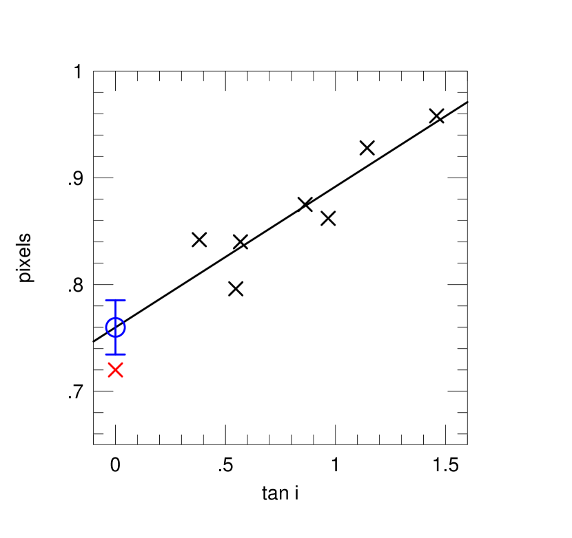
Figure 4: Correction for differential refraction along the east-west axis. Pixel position of the difference-image source in the $x$ (west) direction as a function of $\tan i$, where $i$ is the angle of incidence (i.e., airmass = $\sec i$) at seven epochs (black). The red point shows the position of the “baseline object” on the template. The line is a simple regression of the seven points, while the blue circle is its extrapolation to the zenith. The agreement within 0.04 pixels (16 mas), together with similar agreement on $y$ (north-south) axis, which is not impacted by differential refraction, shows that the blended light is either the lens itself or a companion to the lens. The scatter of the measurements is 10 mas. This strong differential fraction is unusual for the near-standard KMT $I$-band filter and occurs only because of the extreme reddening, which displaces the mean source light from the mean reference-frame light within this filter by $\Delta\lambda=(41\pm 9)\,$nm.

Figure 4 shows the seven measurements of the $x$ (east-west) coordinate of the source position in pixels versus $\tan i$ in black and the “baseline object” position in red. The line is a simple regression without outlier removal. The scatter about this line is $\sigma=10\,{\rm mas}$ (0.025 pixels). The $y$ intercept is the extrapolation of the observed trend to the zenith. The offset from the “baseline object” is only $16\,{\rm mas}$ (0.04 pixels), i.e., of order the error in measuring its position on the template. The offset in the other (north-south) coordinate (which is not significantly affected by differential refraction) is likewise $16\,{\rm mas}$. We note that the slope of the line is $d\theta/d\tan i=(2.56\pm 0.54)\times 10^{-7}\,$radians. Substituting $dn/d\lambda=-6.17\times 10^{-9}\,{\rm nm}^{-1}$, into Equation (8) yields

$$\Delta\lambda=\lambda_{\rm source}-\lambda_{\rm frame}=(41\pm 9)\,{\rm nm}.$$ (9)

The close proximity of the baseline object with the source implies that the excess light is almost certainly associated with the event, i.e., it is either the lens itself or a companion to the lens or to the source. That is, the surface density of stars brighter in $I$ than the blend is only $90\,{\rm arcmin}^{-2}$. Hence, the chance of a random alignment of such a star with the source within $25\,{\rm mas}$ is only $\sim 5\times 10^{-5}$. However, the blend is far too blue to be a companion to the source, which would require that it be behind the same $E(V-I)\sim 4$ column of dust.

5.2 Is the Blend a Companion to the Lens?

Thus, the blend must be either the lens or a companion to the lens. To evaluate the relative probability of these two options, we should consider the matter from the standpoint of the blend, which is definitely in the lens system whether it is the lens or not. There is a roughly 70% probability that the blend has a companion, and if it does, some probability that this companion to the blend is the lens.

However, this conditional probability is actually quite low due to three factors. We express the arguments in terms of $Q\gtrsim 1$, the mass ratio of the blend to the host-lens (viewed as companion to the blend) and $a_{b}$, the projected separation between them. For purposes of this argument, we assume that the lens is at $D_{L}\sim 3\,{\rm kpc}$, but the final result depends only weakly on this choice.

First, $a_{b}<75\,{\rm AU}$. Otherwise the astrometric offset between the source and the “baseline object” would be larger than observed. Second, the source must pass no closer than about 2.5 blend-Einstein-radii from the blend. Expressed quantitatively: $a_{b}>2.5\,D_{L}\,\theta_{\rm E}Q^{1/2}$. Smaller separations can be divided into two cases. Case 1: $0.5\,D_{L}\,\theta_{\rm E}Q^{1/2}\lesssim a_{b}<2.5\,D_{L}\,\theta_{\rm E}Q^{1/2}$. In this case,the blend would give recognizable microlensing signatures to the light curve. Actually, this is a fairly conservative limit because such signatures will often be present even at larger separations. Case 2: $a_{b}\lesssim 0.5\,D_{L}\,\theta_{\rm E}Q^{1/2}$. Such cases are possible, but the planet would then be a circumbinary planet rather than a planet of the companion to the blend, which would be required to make the blend a distinct source of light. Third, the cross section for lensing is lower for the blend’s putative companion than for the blend itself by $Q^{-1/2}$. We take account of all three factors using the binary statistics of Duquennoy & Mayor (1991) and plot the cumulative probability as a function of host to blend mass ratio in Figure 5. The total probability that the blend is a companion to the lens is only 6.6%.

5.3 Gaia Proper Motion of the “Baseline Object”

Regardless of whether the blend is the lens or a companion to the lens, the blend proper motion ${\mbox{\boldmath$\mu$}}_{b}$ is essentially the same as that of the lens. In principle, the two could differ due to orbital motion. However, we argued in Section 5.2 that the projected separation is at least $a_{b}\gtrsim 12Q^{1/2}\,{\rm AU}$, meaning that the velocity of the blend relative to the center of mass of the system is less than $5\,{\rm km}\,{\rm s}^{-1}$, which is small compared to the measurement errors in the problem.

The proper motion of the “baseline object” has been measured by Gaia

$${\mbox{\boldmath$\mu$}}_{\rm base}(N,E)=(-3.0,+0.9)\pm(0.8,1.1)\,{\rm mas}\,{\rm yr}^{-1},$$ (10)

with a correlation coefficient of 0.51. In fact, ${\mbox{\boldmath$\mu$}}_{\rm base}$ is the flux weighted proper motion of the blend and source in the Gaia band,

$${\mbox{\boldmath$\mu$}}_{\rm base}=(1-\eta){\mbox{\boldmath$\mu$}}_{B}+\eta{\mbox{\boldmath$\mu$}}_{S}\rightarrow(1-\eta){\mbox{\boldmath$\mu$}}_{L}+\eta{\mbox{\boldmath$\mu$}}_{S}$$ (11)

where $\eta$ is the fraction of total Gaia flux due to the source. It may eventually be possible to measure $\eta$ directly from Gaia data because there are two somewhat magnified ($A\simeq 1.34$) epochs at ${\rm JD}^{\prime}=8342.62$ and 8342.69 and one moderately magnified ($A\simeq 1.75$) epoch at 8364.62. Based on the reported photometric error and number of observations, we estimate that individual Gaia measurements of the “baseline object” have 2% precision. If so, Gaia will determine $\eta$ with fractional precision $\sigma(\eta)/\eta\simeq 0.022/\eta$. Pending release of Gaia individual-epoch photometry, we estimate $\eta$ by first noting that the blend is 0.32 mag brighter than the source, even in the $I$ band, and that only the blend will effectively contribute at shorter wavelengths where the Gaia passband peaks. We therefore estimate that the blend will contribute an equal number of photons at these shorter wavelengths, while the source will contribute almost nothing, which implies $\eta=0.27$.

We can relate the Gaia proper motion to the heliocentric proper motions of the source and lens by writing

$${\mbox{\boldmath$\mu$}}_{\rm hel}\equiv{\mbox{\boldmath$\mu$}}_{L}-{\mbox{\boldmath$\mu$}}_{S};\qquad{\mbox{\boldmath$\mu$}}_{\rm hel}={\mbox{\boldmath$\mu$}}_{\rm rel}+{\pi_{\rm rel}\over{\rm AU}}{\bf v}_{\oplus,\perp},$$ (12)

where ${\bf v}_{\oplus,\perp}(N,E)=(-3.9,-15.0)\,{\rm km}\,{\rm s}^{-1}$ is Earth’s velocity projected on the event at $t_{0}$. We can then simultaneously solve Equations (11) and (12) to obtain

$${\mbox{\boldmath$\mu$}}_{L}=\eta{\mbox{\boldmath$\mu$}}_{\rm hel}+{\mbox{\boldmath$\mu$}}_{\rm base};\qquad{\mbox{\boldmath$\mu$}}_{S}=-(1-\eta){\mbox{\boldmath$\mu$}}_{\rm hel}+{\mbox{\boldmath$\mu$}}_{\rm base}.$$ (13)

Next, we note that Equation (13) depends only weakly on the somewhat uncertain $\pi_{\rm rel}$ via the ${\bf v}_{\oplus,\perp}$ term in Equation (12). For example, if $\pi_{\rm rel}=0.22\,{\rm mas}$, then this term is only $v_{\oplus,\perp}\pi_{\rm rel}/{\rm AU}\sim 0.7\,{\rm mas}\,{\rm yr}^{-1}$, which is quite small compared to $\mu_{\rm rel}$. Therefore, to simplify what follows, we evaluate ${\mbox{\boldmath$\mu$}}_{\rm hel}$ using this value.

6 A New Test of the ${\mbox{\boldmath$\pi$}}_{\rm E}$ Measurement

The Gaia measurement of the “baseline object” and the resulting Equation (13) allow us to test the reliability of the parallax measurement. Such tests are always valuable, but especially so in the present case because the modeling of the source variability could introduce systematic errors into the parallax measurement. We have already conducted one test by showing in Table 2 that ${\mbox{\boldmath$\pi$}}_{\rm E}$ does not significantly change as we introduce additional wave-form parameters. However, the opportunity for additional tests is certainly welcome, particularly because introducing ${\mbox{\boldmath$\pi$}}_{\rm E}$ only improves the fit by $\Delta\chi^{2}=13$.

From a mathematical standpoint, the two degrees of freedom of ${\mbox{\boldmath$\pi$}}_{\rm E}$ can be equally well expressed in Cartesian $(\pi_{{\rm E},N},\pi_{{\rm E},E})$ or in polar $(\pi_{\rm E},\phi_{\pi})$ coordinates. Here, $\tan\phi_{\pi}\equiv\pi_{{\rm E},E}/\pi_{{\rm E},N}$, i.e., the position angle of ${\mbox{\boldmath$\mu$}}_{\rm rel}$ north through east. Cartesian coordinates are usually more convenient for light-curve modeling because their covariances are better behaved (but see Shin et al. 2018). However, from a physical standpoint, polar coordinates are more useful because the amplitude of ${\mbox{\boldmath$\pi$}}_{\rm E}$ contains all the information relevant to $M$ and $\pi_{\rm rel}$ (see Equation (3)) while the direction contains none. In particular, a test of the measurement of $\phi_{\pi}$ that does not involve any significant assumption about $\pi_{\rm E}$ can give added confidence to the measurement of the latter.

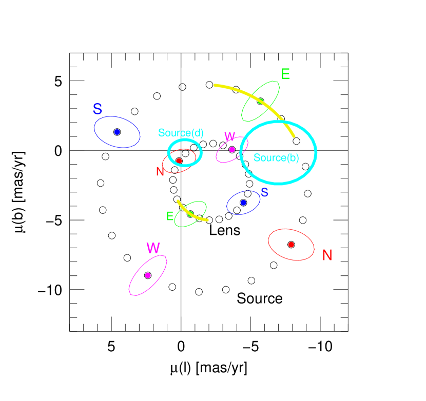
Figure 6: Proper motion of the lens and source, under the assumption that the angle of the parallax vector ${\mbox{\boldmath$\pi$}}_{\rm E}$ has a direction indicated by the figure labels, north (red), east (green), south (blue), and west (magenta), with $15^{\circ}$ steps indicated by black circles. The error ellipses, which take account of both the Gaia errors and correlation coefficient and the error in the magnitude of the geocentric lens-source relative proper motion, $\mu_{\rm rel}$, are shown for the cardinal directions. The cyan ellipses show the expected proper motion dispersions for disk (left) and bar (right) sources. The $1\,\sigma$ range of the measured source proper motion (upper yellow track), which is derived from the direction $\phi_{\pi}$ of the microlens parallax ${\mbox{\boldmath$\pi$}}_{\rm E}$, is consistent with the kinematics of the Galactic-bar. This lends support to the other polar coordinate of the parallax vector, i.e., its amplitude $\pi_{\rm E}$, being correctly measured as well.

Figure 6 illustrates such a test. It shows the source and lens proper motions as functions of $\phi_{\pi}$ in $15^{\circ}$ steps. The cardinal directions are marked in color and labeled. The error ellipses (shown for cardinal directions only) take account of both the Gaia proper motion error and the uncertainty in the magnitude of $\mu_{\rm rel}$ (at fixed direction). The cyan ellipses show the expected dispersions of Galactic-disk (left) and Galactic-bar (right) sources. Hence, it is expected that if the parallax solutions are correct, then at least one of them should yield $\phi_{\pi}$ that is reasonably consistent with one of these two cyan ellipses. Note that there are substantial sections of the source “circle of points” that would be inconsistent or only marginally consistent with these ellipses.

The yellow line segments show the ranges of source (outer) and lens (inner) proper motions implied by the $1\,\sigma$ range of the $\phi_{\pi}$ measurements from the two ($u_{0}>0$ and $u_{0}<0$) solutions. The source proper motion derived from these solutions is clearly consistent with a Galactic bar source. This increases confidence that $\pi_{\rm E}$ is correctly measured within its quoted uncertainties as well.

Finally, we note that in order to limit the complexity of Figure 6, we have fixed both $\pi_{\rm rel}=0.22$ and $\eta=0.27$. We therefore now consider how this Figure would change for other values of these quantities.

Changing $\pi_{\rm rel}$ by $\Delta\pi_{\rm rel}$ would displace the center of each “circle of points” very slightly, i.e., by $-(1-\eta)\Delta\pi_{\rm rel}{\bf v}_{\oplus,\perp}\simeq(0.06,0.23)(\Delta\pi_{\rm rel}/0.1\,{\rm mas}){\rm mas}\,{\rm yr}^{-1}$ for the source and by $(-0.02,0.08)(\Delta\pi_{\rm rel}/0.1\,{\rm mas}){\rm mas}\,{\rm yr}^{-1}$ for the lens. The effect of such a shift on this figure would hardly be discernible.

Changing $\eta$, for example from 0.27 to 0.22 or 0.32, would make the source “circle of points” larger or smaller by 7%. Again, such changes would hardly impact the argument given above.

7 Physical Parameters

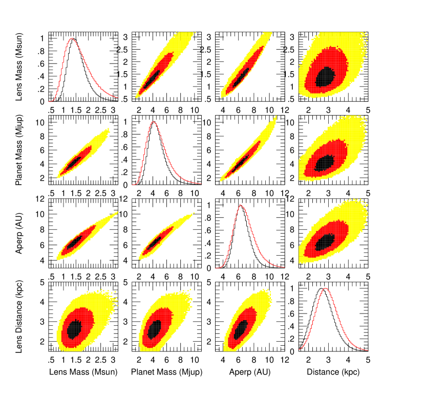
Figure 7: Likelihood distributions for pairs of physical parameters, $(M,M_{p},a_{\perp},D_{L})$, i.e., the lens mass, the planet mass, the host-planet projected separation, and the distance to the lens system. The lower-left panels show the $(u_{0}<0)$ solution, while the upper-right panels show the $(u_{0}>0)$ solution. Black, red, and yellow show likelihood ratios $[-2\Delta\ln({\cal L}/{\cal L}_{\rm max})]<(1,4,9)$, respectively. The diagonal shows the single-parameter histograms, with $(u_{0}<0)$ in black and $(u_{0}>0)$ in red.

While both $\theta_{\rm E}$ and $\pi_{\rm E}$ are measured, they have relatively large fractional errors: of order 20% and 25%, respectively. Hence, it is inappropriate to evaluate the physical parameters simply by algebraically propagating errors, using for example, Equation (3). Instead, we evaluate all physical quantities by applying these (and other) algebraic equations to the output of the MCMC. The results are tabulated in Table 3 and illustrated in Figure 7. Because the source proper motion is consistent with Galactic-bar (but not Galactic-disk) kinematics, we simply assign the source distance $D_{S}=9\,{\rm kpc}$. See Section 6 and Figure 6. The errors are relatively large, but based on the microlensing data alone, the lens is likely to be an F or G star, with a super-Jovian planet.

This result is supported by the fact that the blend (lens) lies near the “bottom edge” (alternatively “blue edge”) of the foreground main-sequences stars on the CMD (Figure 3). To understand the implications of this position, consider two stars of the same apparent color $(V-I)$, but which differ in reddening by $\Delta E(V-I)$ and in intrinsic color by $\Delta(V-I)_{0}$. Tautologically, $\Delta E(V-I)+\Delta(V-I)_{0}=0$. We then adopt estimates $\Delta A_{I}=1.25\Delta E(V-I)$ and $\Delta M_{I}=2.3\Delta(V-I)$. This leads to an estimate

$$\Delta I=\Delta M_{I}+\Delta A_{I}+\Delta{\rm DM}=-0.84\Delta A_{I}+\Delta{\rm DM},$$ (14)

where $\Delta{\rm DM}$ is the difference in distance modulus.

Now, $A_{I}$ is roughly linear in distance $A_{I}=5.2\,{\rm mag}/(9\,{\rm kpc})=0.58\,{\rm mag\,kpc^{-1}}$, while DM is logarithmic, $d{\rm DM}/dD=(5/\ln 10)\,D^{-1}$. Hence, the derivatives of the two terms in Equation (14) are equal and opposite at $D_{\rm stationary}\simeq 4.45\,{\rm kpc}$. As the second derivative of Equation (14) is strictly negative, this stationary point is a maximum. That is, the bottom of the foreground track in the CMD corresponds roughly to stars at this distance, which implies that the lens/blend has $D_{L}\sim D_{\rm stationary}$, $A_{I,L}\sim 2.6$, and $M_{I,L}\sim 2.9$. This would be consistent with an $M\sim 1.5\,M_{\odot}$ main-sequence star, or perhaps a star of somewhat lower mass on the turn off (which is not captured by the simplified formalism of Equation (14)). That is, this qualitative argument is broadly consistent with the results in Table 3. We discuss how followup observations can improve the precision of these estimates in Section 8.2.

We note that at the distances indicated in Figure 7 (or by this more qualitative argument), the lens lies quite close to the Galactic plane,

$$z_{L}=z_{\odot}\biggl{(}1-{D_{L}\over R_{0}}\biggr{)}+D_{L}\sin(b-b_{\rm sgrA*})=-0.0060(D_{L}-2.48\,{\rm kpc}),$$ (15)

where $b_{\rm sgrA*}$ is the Galactic latitude of SgrA*, $R_{0}$ is the Galactocentric distance, and where we have adopted $z_{\odot}=15\,{\rm pc}$ for the height of the Sun above the Galactic plane. That is, if $D_{L}$ is within a kpc of 2.48 kpc, then the lens is within 6 pc, of the Galactic plane.

8 Discussion

8.1 Lowest Galactic-Latitude Planet

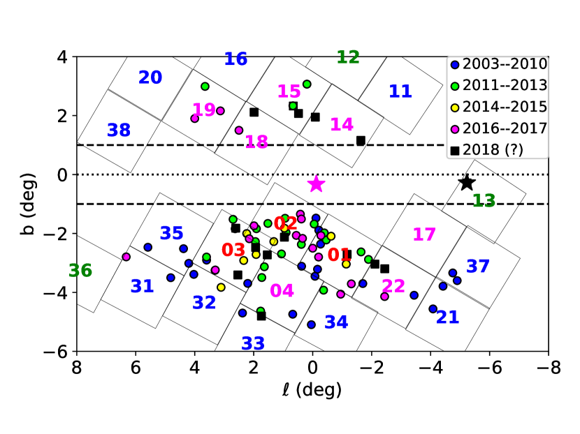
Figure 8: The positions of published microlensing planets from 2003-2017 (circles) and likely-to-be-published microlensing planets from 2018 (squares) are shown against the KMT field configuration for 2016-2018, which are color-coded (red, magenta, blue, green) according to their nominal cadence $\Gamma=(4,1,0.4,0.2)\,{\rm hr}^{-1}$. The two planets that lie close to the plane, UKIRT-2017-BLG-001Lb (Shvartzvald et al., 2018) and KMT-2018-BLG-1292Lb (this work) are shown as stars. Despite the fact that KMT systematically avoids the Galactic plane, five of its fields (BLG13, 14, 18, 38, and 02/42) “inadvertently” cross the plane or come close to it. The detection of KMT-2018-BLG-1292Lb in the lowest cadence of these fields suggests that the Galactic plane could be probed for planets in the optical at relatively low cost. Published planets are color coded by year of discovery. Their changing areal distribution with time is discussed in Section 8.1.

At $b=-0.28$, KMT-2018-BLG-1292Lb is the lowest Galactic-latitude microlensing planet yet detected. Yet, KMTNet did not consciously set out to monitor the Galactic plane. Instead, it has a few fields, including BLG13, BLG14, BLG18, BLG38, and BLG02/BLG42, whose corners “inadvertently” cross the Galactic plane or come very close to it. See Figure 8. This is a side effect of having a large-format square camera on an equatorial mount telescope (together with the fact that the Galactic plane is inclined by $\sim 30^{\circ}$ relative to north toward the Galactic center). Of these five fields, BLG13 has the lowest cadence ($\Gamma=0.15$–$0.2\,{\rm hr}^{-1}$), with BLG14 and BLG18 being 5 times higher and BLG02/42 being 20 times higher. Nevertheless, despite this low-cadence (further aggravated by the fact that the anomaly occurred near the end of the season, when the Galactic bulge was visible for only a few hours per night) and the very high extinction $A_{I}\sim 5.2$, KMT-2018-BLG-1292Lb is reasonably well characterized, with measurements of both $\theta_{\rm E}$ and ${\mbox{\boldmath$\pi$}}_{\rm E}$. This leads us to assess the reason for this serendipitous success.

The first point is that the source is very luminous and very red, which together made the event reasonably bright in spite of the high extinction. It also implies a large source radius, with a source-diameter crossing time of almost one day, $2t_{*}=19\,$hr. Hence, despite the low effective combined cadence from all three observatories $\Gamma\sim 1\,{\rm day}^{-1}$, the source profiles on the source plane nearly overlap as it transits the caustic. See Figure 2. Thus, although the actual trajectory fortuitously rides the edge of a caustic, even random trajectories through the caustic would have led to significant finite source effects for some measurements, and therefore to a measurement of $\theta_{\rm E}$. This large source size is not fortuitous: in high extinction fields, such large sources are the only ones that will give rise to detectable microlensing events in the optical, apart from a handful of very high magnification events. That is, although high-extinction fields necessarily greatly reduce the number of sources that can be probed for microlensing events, those that can shine through the dust can yield well-characterized events even with very low cadence. This means that optical surveys could in principle more systematically probe the Galactic plane for microlens planets at relatively low cost in observing time.

Although Figure 8 is presented primarily to show current optical coverage of the Galactic plane and to illustrate the possibilities for future coverage, it also has more general implications for understanding past and possible future strategies for microlensing planet detection. We summarize these here. The colored circles in Figure 8 represent published microlensing planets discovered in 2003-2017, while the black squares show 2018 event locations that we assess as likely to yield future planet publications. The blue points, which are from 2003-2010, i.e., prior to OGLE-IV, are uniformly distributed over the southern bulge. By contrast (and restricting attention for the moment to the southern bulge) planet detections in all subsequent epochs are far more concentrated toward the regions near $(l,b)\sim(+1,-2.5)$. During 2003-2010, the cadence of the survey observations was typically too low to detect and characterize planets by themselves. Hence, most planets were discovered by a combination of follow-up observations (including survey auto-follow-up) and survey observations of events alerted by OGLE and/or MOA. The choice of these follow-up efforts was not strongly impacted by survey cadence, which in any case was relatively uniform. It is still slightly surprising that the planet detections do not more closely track the underlying event rate, which is higher toward the concentration center of later planet detections.

As soon as the OGLE-IV survey started (green points 2011-2013), the overall detection rate increases by a factor 2.7, but the southern-bulge planets also immediately become more concentrated. This partly reflects that the OGLE and MOA surveys (together with the Wise survey, Shvartzvald et al. 2016) were very capable of detecting planets without followup observations in their higher-cadence regions, which were near this concentration. But in addition, these higher-cadence regions began yielding vastly more alerted events and also better characterization of these events, which also tended to concentrate the targets for follow-up observations. Also notable in this period are the first three planets in the northern bulge, to which OGLE-IV devoted a few relatively high-cadence fields.

In the next period (yellow points, 2014-2015), the surveys remained similar, but follow-up observations were sharply curtailed due to reduction of work by the Microlensing Follow-Up Network ($\mu$FUN, Gould et al. 2010). The rate drops by 45%, but the main points to note are that the southern bulge discoveries become even more concentrated and there are no northern bulge discoveries. In particular, comparing 2003-2010 with 2011-2015, the dispersion in the $l$ direction in the southern bulge drops by more than a factor two, from $3.21^{\circ}\pm 0.50^{\circ}$ to $1.45^{\circ}\pm 0.20^{\circ}$.

The magenta and black points together show the planets discovered during the three years when the KMT wide-area survey joined the ongoing OGLE and MOA surveys, which is also the first time that the KMT fields shown in the figure become relevant to the immediate discussion. There are several points to note. First, the rate of detection increases by a factor 2.7 relative to the previous two years (or by a factor 1.8 relative to the previous five years). Second, the southern bulge planets become somewhat less concentrated, but still tend to follow the KMT very-high-cadence (numbered in red) and high-cadence (numbered in magenta) fields. In fact, only four out of 24 planets in the southern bulge lie outside of these fields. This should be compared to the 22 blue (2003-2010) points, 11 (half) of which lie outside these fields. Finally, there are eight planets in the northern bulge, all in the four high cadence fields.

This history seems to indicate that there is substantial potential for finding microlensing planets in low cadence fields by carrying out aggressive follow-up observations similar to those of the pre-OGLE-IV era.

8.2 Precise Lens Characterization From Spectroscopic Followup

As shown in Section 5.1, the blend is almost certainly either the lens or its companion and as shown in Section 5.2, it is very likely to be the lens. See Figure 5. Hence, a medium-resolution spectrum of the blend would greatly clarify the nature of the lens in two ways.

First, by spectrally typing the blend one could obtain a much better estimate of its mass. Second, if the mass turns out to be, e.g., $M\sim 1.5\,M_{\odot}$ in line with the results in Table 3, then this would further reduce the probability that the lens is a companion to the blend relative to the 6.6% probability that we derived in Section 5.2. This is because companions to the blend with mass ratio $Q^{-1}\lesssim 0.5$ would then have masses $M\lesssim 0.75\,M_{\odot}$, which are significantly disfavored by the results of Section 7. Hence, of order half the probability allowed by Figure 5 would be eliminated, which would further increase confidence that the blend (now spectrally typed) was the lens.

Such a spectrum could be taken immediately. Of course, the source would remain in the aperture for many years, but it is unlikely to contribute much light in the $V$- and $R$-band ranges of the spectrum, as we discussed in Section 5.1. In addition, the source spectrum is likely to be displaced by many tens of ${\rm km}\,{\rm s}^{-1}$ from that of the blend.

Table 1: Best Fit Models of KMT-2018-BLG-1292

			Parallax $(P_{2})$
Parameters	Standard	Standard $(P_{2})$	$u_{0}>0$	$u_{0}<0$
$\chi^{2}/\rm{dof}$	750.637/721	723.357/715	710.145/713	710.294/713
$t_{0}$ $(\rm{HJD}^{\prime})$	8408.91 $\pm$ 0.52	8408.98 $\pm$ 0.52	8408.35 $\pm$ 0.15	8407.91 $\pm$ 0.33
$u_{0}$	0.268 $\pm$ 0.009	0.269 $\pm$ 0.009	0.286 $\pm$ 0.013	-0.281 $\pm$ 0.008
$t_{\rm E}$ $(\rm{days})$	67.33 $\pm$ 1.57	66.48 $\pm$ 1.50	61.87 $\pm$ 2.05	60.80 $\pm$ 1.36
$s$	1.328 $\pm$ 0.009	1.333 $\pm$ 0.009	1.347 $\pm$ 0.013	1.343 $\pm$ 0.008
$q$ $(10^{-3})$	2.671 $\pm$ 0.245	2.705 $\pm$ 0.245	2.852 $\pm$ 0.270	2.982 $\pm$ 0.221
$\alpha$ $(\rm{rad})$	2.595 $\pm$ 0.009	2.601 $\pm$ 0.009	2.576 $\pm$ 0.020	-2.589 $\pm$ 0.020
$\rho$ $(10^{-3})$	5.790 $\pm$ 0.821	5.687 $\pm$ 0.776	6.505 $\pm$ 1.135	6.516 $\pm$ 0.777
$\pi_{\rm{E},\it{N}}$	-	-	0.032 $\pm$ 0.058	-0.021 $\pm$ 0.061
$\pi_{\rm{E},\it{E}}$	-	-	0.118 $\pm$ 0.029	0.131 $\pm$ 0.027
$f_{S}$	0.359 $\pm$ 0.015	0.365 $\pm$ 0.015	0.387 $\pm$ 0.021	0.379 $\pm$ 0.013
$f_{B}$	0.450 $\pm$ 0.015	0.446 $\pm$ 0.014	0.421 $\pm$ 0.021	0.430 $\pm$ 0.014
$t_{*}$ $(\rm{days})$	0.390 $\pm$ 0.049	0.378 $\pm$ 0.046	0.403 $\pm$ 0.061	0.396 $\pm$ 0.044
$a_{1}$		0.012 $\pm$ 0.004	0.008 $\pm$ 0.003	0.010 $\pm$ 0.003
$P_{1}$ $(\rm{days})$	-	70.13 $\pm$ 9.81	62.24 $\pm$ 9.71	63.63 $\pm$ 9.22
$\phi_{1}$	-	0.670 $\pm$ 0.513	0.993 $\pm$ 0.611	0.451 $\pm$ 0.577
$a_{2}$	-	0.009 $\pm$ 0.003	0.007 $\pm$ 0.002	0.007 $\pm$ 0.002
$P_{2}$ $(\rm{days})$	-	13.04 $\pm$ 2.32	13.00 $\pm$ 4.90	13.00 $\pm$ 6.85
$\phi_{2}$	-	-0.070 $\pm$ 0.324	-0.450 $\pm$ 0.549	0.076 $\pm$ 0.773

Table 2: Parameter Evolution with Additional Periodic Components

Parameters	$P_{0}$	$P_{1}$	$P_{2}$
$\rm{Parallax}(u_{0}>0)$
$\chi^{2}/\rm{dof}$	731.918/719	719.868/716	710.145/713
$q$ $(10^{-3})$	2.781 $\pm$ 0.240	2.865 $\pm$ 0.223	2.852 $\pm$ 0.270
$\rho$ $(10^{-3})$	5.809 $\pm$ 0.871	5.433 $\pm$ 0.831	6.505 $\pm$ 1.135
$f_{S}$	0.363 $\pm$ 0.015	0.368 $\pm$ 0.015	0.387 $\pm$ 0.021
$\pi_{\rm{E},\it{N}}$	0.0002 $\pm$ 0.053	0.088 $\pm$ 0.058	0.032 $\pm$ 0.058
$\pi_{\rm{E},\it{E}}$	0.105 $\pm$ 0.027	0.119 $\pm$ 0.028	0.118 $\pm$ 0.029
$a_{1}$	-	0.009 $\pm$ 0.003	0.008 $\pm$ 0.003
$P_{1}$ $(\rm{days})$	-	62.17 $\pm$ 9.26	62.24 $\pm$ 9.71
$\phi_{1}$	-	0.705 $\pm$ 1.234	0.993 $\pm$ 0.611
$a_{2}$	-	-	0.007 $\pm$ 0.002
$P_{2}$ $(\rm{days})$	-	-	13.00 $\pm$ 4.90
$\phi_{2}$	-	-	-0.450 $\pm$ 0.549
$\rm{Parallax}(u_{0}<0)$
$\chi^{2}/\rm{dof}$	732.186/719	719.252/716	710.294/713
$q$ $(10^{-3})$	2.937 $\pm$ 0.247	3.117 $\pm$ 0.236	2.982 $\pm$ 0.221
$\rho$ $(10^{-3})$	6.083 $\pm$ 0.930	6.728 $\pm$ 0.909	6.516 $\pm$ 0.777
$f_{S}$	0.368 $\pm$ 0.016	0.381 $\pm$ 0.016	0.379 $\pm$ 0.013
$\pi_{\rm{E},\it{N}}$	0.003 $\pm$ 0.054	-0.008 $\pm$ 0.058	-0.021 $\pm$ 0.061
$\pi_{\rm{E},\it{E}}$	0.118 $\pm$ 0.028	0.129 $\pm$ 0.027	0.131 $\pm$ 0.027
$a_{1}$	-	0.008 $\pm$ 0.003	0.010 $\pm$ 0.003
$P_{1}$ $(\rm{days})$	-	62.67 $\pm$ 13.16	63.63 $\pm$ 9.22
$\phi_{1}$	-	0.453 $\pm$ 1.346	0.451 $\pm$ 0.577
$a_{2}$	-	-	0.007 $\pm$ 0.002
$P_{2}$ $(\rm{days})$	-	-	13.00 $\pm$ 6.85
$\phi_{2}$	-	-	0.076 $\pm$ 0.773

Table 3: Physical parameters

	Parallax $(P_{2})$
Quantity	$u_{0}>0$	$u_{0}<0$
$M_{\rm lens}$ $[M_{\sun}]$	$1.54_{-0.43}^{+0.67}$	$1.51_{-0.30}^{+0.41}$
$M_{\rm planet}$ $[M_{J}]$	$4.53_{-1.26}^{+1.79}$	$4.45_{-0.98}^{+1.32}$
$a_{\bot}$ [au]	$6.65_{-1.14}^{+1.47}$	$6.41_{-0.88}^{+1.07}$
${\it D_{L}}$ [kpc]	$2.92_{-0.54}^{+0.62}$	$2.69_{-0.51}^{+0.58}$
$\theta_{\rm{E}}$ [mas]	$1.71_{-0.26}^{+0.34}$	$1.80_{-0.23}^{+0.28}$
$\mu_{{\rm hel},N}$ [mas/yr]	$3.6_{-4.5}^{+2.9}$	$-5.2_{-3.5}^{+4.8}$
$\mu_{{\rm hel},E}$ [mas/yr]	$8.1_{-1.8}^{+1.8}$	$8.2_{-2.3}^{+1.7}$
$v_{{\rm L,LSR},l}$ [km/s]	$9.5_{-12.5}^{+6.6}$	$-13.0_{-9.8}^{+14.0}$
$v_{{\rm L,LSR},b}$ [km/s]	$-44.7_{-17.3}^{+17.0}$	$-52.4_{-11.0}^{+10.2}$

Figure 5: Cumulative probability that the host is a companion to the blend (rather than the blend itself) as function of lens to “putative primary” (blend) mass ratio. Although lower mass secondaries of G-dwarf binaries are more common (Duquennoy & Mayor, 1991), these are suppressed by lower cross sections ($\propto M^{1/2}$) and smaller range of semi-major axis in which the “putative primary” could avoid giving rise to microlensing signatures. The total probability that the lens is a companion to the blend (rather than the blend itself) is only 6.6%.

References

- Alard & Lupton (1998) Alard, C. & Lupton, R.H.,1998, ApJ, 503, 325
- Albrow et al. (2009) Albrow, M. D., Horne, K., Bramich, D. M., et al. 2009, MNRAS, 397, 2099
- An & Gould (2001) An, J.H., & Gould, A. 2001, ApJ, 563, L111
- Batista et al. (2011) Batista, V., Gould, A., Dieters, S. et al. A&A, 529, 102
- Bennett et al. (2008) Bennett, D.P., Bond, I.A., Udalski, A., et al. 2008, ApJ, 684, 663
- Bennett et al. (2012) Bennett, D.P., Sumi, T., Bond, I.A., et al. 2012, ApJ, 757, 119
- Bensby et al. (2013) Bensby, T. Yee, J.C., Feltzing, S. et al. 2013, A&A, 549A, 147
- Bessell & Brett (1988) Bessell, M.S., & Brett, J.M. 1988, PASP, 100, 1134
- DePoy et al. (2003) DePoy, D.L., Atwood, B., Belville, S.R., et al. 2003, SPIE 4841, 827
- Duquennoy & Mayor (1991) Duquennoy, A., & Mayor, M. 1991, A&A, 248, 485
- Gould (1992) Gould, A. 1992, ApJ, 392, 442
- Gould (1995) Gould, A. 1995, ApJ, 446, L71
- Gould (2000) Gould, A. 2000, ApJ, 542, 785
- Gould & Loeb (1992) Gould, A. & Loeb, A. 1992, ApJ, 396, 104
- Gould et al. (2010) Gould, A., Dong, S., Gaudi, B.S. et al. 2010, ApJ, 720, 1073
- Groenewegen (2004) Groenewegen, M.A.T., 2004, MNRAS, 353, 903
- Kim et al. (2016) Kim, S.-L., Lee, C.-U., Park, B.-G., et al. 2016, JKAS, 49, 37
- Kim et al. (2018a) Kim, D.-J., Kim, H.-W., Hwang, K.-H., et al., 2018a, AJ, 155, 76
- Koshimoto et al. (2014) Koshimoto1, N., Udalski2, A., Sumi, T., et al. 2014, AJ, 788, 128
- Minniti et al. (2010) Minniti, D., Lucas, P. W., Emerson, J. P., et al. 2010, New Astron., 15, 433
- Minniti (2018) Minniti, D. 2018, in The Vatican Observatory, Castel Gandolfo: 80th Anniversary Celebration (ed. G. Gionti, S.J., & J.-B. Kikwaya Eluo, S.J). Astrophysics and Space Science Proceedings, 51, 63
- Nataf et al. (2013) Nataf, D.M., Gould, A., Fouqué, P. et al. 2013, ApJ, 769, 88
- Navarro et al. (2017) Navarro, M.G., Minniti, D., & Contreras-Ramos, R. 2017, ApJ, 851, L13
- Navarro et al. (2018) Navarro, M.G., Minniti, D., & Contreras-Ramos, R. 2018, ApJ, 865, L5
- Navarro et al. (2019) Navarro, M.G., Minniti, D., & Contreras-Ramos, R. 2019, submitted
- Paczyński (1986) Paczyński, B. 1986, ApJ, 304, 1
- Poleski et al. (2014a) Poleski, R., Skowron, J., Udalski, A., et al. 2014a, ApJ, 755, 42
- Poleski (2016) Poleski, R. 2016, MNRAS, 455, 3656
- Rattenbury et al. (2015) Rattenbury, N.J., Bennett, D.P., Sumi, T., et al. 2015, MNRAS, 454, 946
- Saito et al. (2012) Saito, R.K., Hempel, M., Minniti, D., et al. 2012, A&A, 537, A107
- Shin et al. (2018) Shin, I.-G., Yee, J.C., Skowron, J. et al. 2018, ApJ, 863, 23
- Shvartzvald et al. (2016) Shvartzvald, Y., Maoz, D., Udalski, A. et al. 2016, MNRAS, 457, 4089
- Shvartzvald et al. (2017) Shvartzvald, Y.,Bryden, G., Gould, A., et al. 2017, AJ, 153, 61
- Shvartzvald et al. (2018) Shvartzvald, Y., Calchi Novati, S., Gaudi, B.S., et al. 2018, ApJ, 857, 8
- Skowron et al. (2011) Skowron, J., Udalski, A., Gould, A et al. 2011, ApJ, 738, 87
- Suzuki et al. (2014) Suzuki, D., Udalski, A., Sumi, T., et al. 2014, ApJ, 780, 123
- Udalski et al. (2015a) Udalski, A., Syzmanski, M.K., & Szymanski, G., et al. 2015a, AcA, 65, 1
- Woźniak (2000) Woźniak, P. R. 2000, Acta Astron., 50, 421
- Yoo et al. (2004) Yoo, J., DePoy, D.L., Gal-Yam, A. et al. 2004, ApJ, 603, 139