Higgs boson decay into four bottom quarks in the SM and beyond

Abstract

We present predictions for the Higgs boson decay into four bottom quarks in the standard model and via light exotic scalars retaining full bottom-quark mass dependence. In the SM the decay can be induced either by the Yukawa couplings of bottom quarks and top quarks or the electroweak couplings. We calculate the partial decay width and various differential distributions up to next-to-leading order in QCD. We find large QCD corrections for decay via Yukawa couplings, as large as 90% for the partial decay width, and reduced scale variations. The results of this paper are therefore helpful for the measurement of this multi-jets final state at future Higgs factory of electron-positron colliders. We also propose several observables that can differentiate the SM decay channel and the exotic decay channel and compare their next-to-leading order predictions.

1 Introduction

The successful operation of the LHC and the ATLAS and CMS experiments have led to the discovery of the Higgs boson and completion of the standard model (SM) of particle physics Aad:2012tfa ; Chatrchyan:2012xdj . Further refined study at the LHC has revealed one essential of the Higgs boson, Yukawa couplings of top quarks Sirunyan:2018hoz ; Aaboud:2018urx and bottom quarks Aaboud:2018zhk ; Sirunyan:2018kst . Precision test on properties of the Higgs boson including all its couplings with standard model particles becomes one primary task of particle physics at the high energy frontier. In the SM the Higgs boson decays dominantly to hadronic final states which are hard to access at hadron colliders due to huge QCD backgrounds. That includes decay channels of a pair of bottom quarks or charm quarks, a pair of gluons via top-quark loops, and four quarks via electroweak gauge bosons, adding to a total decay branching ratio of about 80% 1307.1347 . To measure the Higgs properties with higher accuracy and to probe rare decay modes of the Higgs boson, there have been a few proposals to build a future lepton collider that can serve as a Higgs factory. These include ILC Behnke:2013xla , CEPC CEPCStudyGroup:2018ghi , CLIC Lebrun:2012hj and FCC-$ee$ Gomez-Ceballos:2013zzn . The proposed LHeC program can also produce abundant Higgs boson and measure its couplings precisely 1206.2913 ; Klein:2018rhq . Certainly with the future Higgs factory, the precious hadronic decay channles of the Higgs boson can be studied in details thanks to the clean environment An:2018dwb .

Precision experiments require equally precision theoretical predictions. To further scrutinize the SM and to look for possible new physics beyond, it is necessary to calculate higher-order corrections to the production and decay of the Higgs boson. In this respect, there have been enormous advances in recent years. For example, the next-to-next-to-next-to-leading order (N³LO) QCD corrections to Higgs boson production via gluon fusion in the heavy top-quark limit Anastasiou:2015ema ; Mistlberger:2018etf and to Higgs boson production via vector boson fusion within the structure function approach Dreyer:2016oyx , the next-to-next-to-leading order (NNLO) corrections to Higgs boson production in association with a jet in the heavy top-quark limit Boughezal:2013uia ; Chen:2014gva ; Boughezal:2015dra ; Boughezal:2015aha , and the next-to-leading order (NLO) corrections to Higgs boson pair production with full top-quark mass dependence Borowka:2016ypz have been known for some time. The two-loop mixed QCD and electroweak corrections have also been calculated recently for the associated production of Higgs boson and a $Z$ boson at electron-positron colliders Gong:2016jys ; Sun:2016bel ; Chen:2018xau . For decays of the Higgs boson, the partial width for $H\to b\bar{b}$ is known up to the next-to-next-to-next-to-next-to-leading order (N⁴LO), in the limit where the mass of the bottom quark is neglected Baikov:2005rw ; Davies:2017xsp ; Herzog:2017dtz . The partial width for $H\to gg$ has been calculated to the N³LO Baikov:2006ch and N⁴LO Herzog:2017dtz in the heavy top-quark limit. We refer the readers to Denner:2011mq ; Spira:2016ztx for a complete list of relevant calculations. At a more exclusive level, the fully differential cross sections for $H\to b\bar{b}$ have been calculated to NNLO in Anastasiou:2011qx ; DelDuca:2015zqa and N³LO in Mondini:2019gid for massless bottom quarks, and to NNLO in Bernreuther:2018ynm with massive bottom quarks.

Besides, multi-jets final state, for instance, Higgs boson decays into three or four QCD partons can also be explored at future Higgs factory. There have been strong motivations for experimental searches of those exclusive hadronic decay channels to look for exotic decays of the Higgs boson induced by light states beyond the SM 0909.1521 ; 1312.4992 ; Liu:2016zki ; Liu:2016ahc . Among them there is the decay of the Higgs boson to four bottom quarks which will be the main focus of this paper. There have already been searches carried out by ATLAS collaboration at the LHC 1806.07355 setting an upper limit of about 50% on the decay branching ratio to four bottom quarks. On the theory side, the Higgs boson decays into four massless quarks via electroweak gauge bosons have been calculated to NLO in both QCD and electroweak couplings and have been implemented in the MC program Prophecy4f Bredenstein:2006rh ; Bredenstein:2006ha . There have also been recent predictions for Higgs boson decays into three-jets final state Li:2018qiy ; 1901.02253 ; 1903.07277 for the hadronic event shapes. That is particularly interested for the probe of light-quark Yukawa interactions Gao:2016jcm . Very recently there exist a NNLO calculation for Higgs boson decays into a pair of bottom quarks plus an additional jet for massless bottom quarks Mondini:2019vub .

In this paper, we present predictions for the Higgs boson decays into four bottom quarks in the standard model and via light exotic scalars retaining full bottom-quark mass dependence. In the SM the decays can be induced either by the Yukawa couplings of bottom quarks and top quarks or the electroweak couplings. We calculate the partial decay width and various differential distributions up to next-to-leading order in QCD. We discuss details of the calculation in Section 2 and present numerical results for the SM case. We then move to discussion on exotic decays induced by new scalars including for the QCD corrections and comparisons to the SM case in Section 3. We conclude in Section 4.

2 Decay in the SM

2.1 Decay via Yukawa interactions

In the full theory with $n_{f}=6$ active flavor of quarks, the relevant interactions include the Yukawa couplings of quarks and the QCD interactions,

$$\mathcal{L}_{int}=\mathcal{L}_{QCD}-\sum_{i=n_{f}-1}^{n_{f}}\frac{H}{v}m_{i}\bar{\psi}_{i}\psi_{i},$$ (1)

We neglect quark masses except for top quark and bottom quark. We use onshell scheme for renormalization of the quark or gluon fields and masses except for masses in Yukawa couplings, when calculating the QCD radiative corrections. The renormalization of the QCD coupling is carried out in $\overline{\rm MS}$ scheme with top quark decoupled Collins:1978wz , namely the number of light and heavy flavor, $n_{l}=5$ and $n_{h}=1$ respectively. The corresponding renormalization constants at one-loop are,

$$Z_{g} = 1+\frac{\alpha_{S}^{(n_{l})}(\mu)}{4\pi}S_{\epsilon}\left\{-\frac{\beta_{0}^{(n_{l})}}{\epsilon}+\frac{2T_{R}}{3\epsilon}\sum_{i=n_{f}-n_{h}+1}^{n_{f}}\left(\frac{\mu^{2}}{m_{i}^{2}}\right)^{\epsilon}\right\},$$

$$Z_{2}^{G} = 1-\frac{\alpha_{S}^{(n_{l})}(\mu)}{4\pi}S_{\epsilon}\frac{4T_{R}}{3\epsilon}\sum_{i=n_{f}-n_{h}+1}^{n_{f}}\left(\frac{\mu^{2}}{m_{i}^{2}}\right)^{\epsilon},$$

$$Z_{2}^{\psi_{i}} = 1-\frac{\alpha_{S}^{(n_{l})}(\mu)}{4\pi}S_{\epsilon}C_{F}\left\{\frac{3}{\epsilon}+4\right\}\left(\frac{\mu^{2}}{m_{i}^{2}}\right)^{\epsilon},$$

$$\frac{\delta m_{i}}{m_{i}} = -\frac{\alpha_{S}^{(n_{l})}(\mu)}{4\pi}S_{\epsilon}C_{F}\left\{{\frac{3}{\epsilon}+4}\right\}\left(\frac{\mu^{2}}{m_{i}^{2}}\right)^{\epsilon},$$ (2)

with $S_{\epsilon}=(4\pi)^{\epsilon}/\Gamma(1-\epsilon)$, and $\beta_{0}^{(n_{l})}=(11C_{A}-4T_{R}n_{l})/6$. Furthermore, since the relevant hard scale is much larger than the bottom quark mass, we use the $\overline{\rm MS}$ running mass of bottom quark in Yukawa coupling, that can be related to the input pole mass hep-ph/0004189 .

Since the top quarks only appear as internal states, one can adopt an effective theory by integrating out top quark, the interactions can be expressed as

$$\mathcal{L}_{eff}=\mathcal{L}_{QCD}-\frac{H}{v}C_{1}G_{\mu\nu}^{a}G^{\mu\nu,a}-\frac{H}{v}C_{2}\sum_{i=n_{l}}^{n_{l}}m_{i}\bar{\psi}_{i}\psi_{i},$$ (3)

to the leading power of inverse of the top-quark mass. The Wilson coefficients $C_{1}$ and $C_{2}$ Kataev:1981gr ; Inami:1982xt ; Dawson:1990zj ; Djouadi:1991tka ; Kataev:1993be ; hep-ph/9405325 ; Spira:1995rr ; hep-ph/9708255 carry further logarithmic dependence on top-quark mass and are given by

$$C_{1} = -\frac{\alpha_{S}^{(n_{l})}(\mu)}{12\pi}\left\{1+\frac{\alpha_{S}^{(n_{l})}(\mu)}{4\pi}11+\mathcal{O}(\alpha_{S}^{2})\right\},$$

$$C_{2} = 1+\left(\frac{\alpha_{S}^{(n_{l})}(\mu)}{4\pi}\right)^{2}\left\{{40\over 9}-{16\over 3}\log{\mu^{2}\over m_{t}^{2}}\right\}+\mathcal{O}(\alpha_{S}^{3}).$$ (4)

The renormalization of QCD coupling and gluon field are done with pure $\overline{\rm MS}$ scheme with $n_{l}=5$ light flavors. Again we use onshell scheme for renormalization of bottom quark field and mass, apart from using $\overline{\rm MS}$ running mass in the Yukawa coupling. That is equivalent to set $n_{h}=0$ in Eq. (2.1). Moreover, in the effective theory, there will be operator mixing between the last two terms in Eq. (3) requiring renormalization of the Wilson coefficients,

$$C_{1}^{0}=Z_{11}C_{1},\quad\quad C_{2}^{0}=Z_{21}C_{1}+C_{2},$$ (5)

with the one-loop renormalization constants in $\overline{\rm MS}$ scheme given by hep-ph/9708255 ,

$$Z_{11} = 1-\frac{\alpha_{S}^{(n_{l})}(\mu)}{4\pi}S_{\epsilon}\frac{2\beta_{0}^{(n_{l})}}{\epsilon},$$

$$Z_{21} = -\frac{\alpha_{S}^{(n_{l})}(\mu)}{4\pi}S_{\epsilon}\frac{12C_{F}}{\epsilon}.$$ (6)

Under the effective theory the leading order (LO) Feynman diagrams for the Higgs boson decaying into four bottom quarks are shown in Fig. 1. Those diagrams can be obtained with interchanges of identical particles are not shown for simplicity. In this calculation the squared amplitudes needed for a next-to-leading order QCD calculation are generated automatically with program GoSam 2.0 1404.7096 , including for the one-loop virtual corrections and the real corrections. Reduction of loop integrals are performed with Ninja 1203.0291 ; 1403.1229 and scalar integrals are calculated with OneLOop 0903.4665 ; 1007.4716 . We do not show here the one-loop virtual or real radiation diagrams which are lengthy. We use the dipole subtraction method with massive quarks hep-ph/0201036 for handling the QCD real corrections.

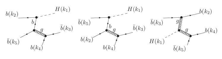
Figure 1: Feynman diagrams at leading order for the Higgs boson decaying into four bottom quarks via Yukawa interactions. Diagrams can be obtained with interchanges of identical particles are not shown for simplicity.

2.2 Decay via electroweak interactions

Within the standard model, the Higgs boson can also decay into four bottom quarks through a cascade decay with an onshell $Z$ boson, $H\rightarrow Z(b\bar{b})b\bar{b}$. The corresponding branching ratio turns to be comparable to the one as induced by the Yukawa couplings of bottom quarks and top quarks. At leading order the relevant Feynman diagrams in Feynman-’t Hooft gauge are shown in Fig. 2. Those diagrams mediated by $Z$ boson and goldstone bosons $\chi$ must be considered together to form a gauge invariant set. Furthermore, we also include the diagrams mediated by Higgs bosons though their contributions are small, since we would like to keep full bottom quark mass dependence. In principle there are also Feynman diagrams mediated by photons. We do not consider them here since there at next-to-leading order in QCD one will also need to include one-loop QED corrections of decay via Yukawa couplings for consistency.

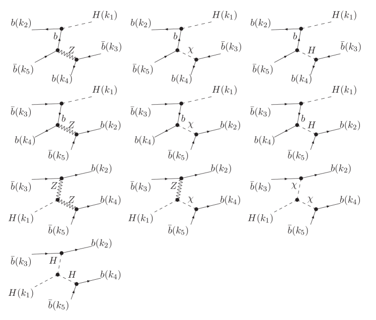
Figure 2: Similar to Fig. 1 for Feynman diagrams of the Higgs boson decaying into four bottom quarks via electroweak interactions.

As mentioned earlier dominant contributions to decay via electroweak couplings arise from the resonance region, namely one of the $b\bar{b}$ pairs lies at $Z$ boson mass pole. Thus one must include finite width effects of the electroweak gauge bosons which may violate gauge symmetry since that will mix contributions from various orders of the EW couplings. In order to preserve gauge symmetry especially at one-loop level in QCD, we use the complex mass scheme hep-ph/0505042 . There the masses of $W$ and $Z$ bosons and the electroweak couplings are complex numbers depending on the width of $W$ and $Z$ bosons, and the Lagrangian are manifestly gauge invariant. The squared amplitudes needed for the next-to-leading order QCD calculation are again generated automatically with GoSam 2.0 1404.7096 and are checked against MadGraph5_aMC@NLO 1405.0301 . Good agreements are found between the two programs.

2.3 Inclusive decay rate

Similar to the total hadronic width, the inclusive decay width of the Higgs boson to four bottom quarks in the limit of infinite top-quark mass includes contributions from the bottom-quark Yukawa coupling, the gluon effective coupling, and their interferences. It can be expressed as hep-ph/0503172

$$\Gamma_{4b,yuk} = \left(\frac{\alpha_{S}(\mu)}{2\pi}\right)^{2}\Big{\{}A_{b\bar{b}}[\Delta_{b\bar{b}}(x)(1+\delta_{b\bar{b}}(x))C_{2}^{2}+\Delta_{bg}(x)(1+\delta_{bg}(x))C_{1}C_{2}]$$ (7)

$$+A_{gg}[\Delta_{gg}(x)(1+\delta_{gg}(x))C_{1}^{2}]\Big{\}},$$

with

$$A_{b\bar{b}}=\frac{3M_{H}}{8\pi v^{2}}\overline{m}_{b}^{2}(\mu),\qquad A_{gg}=\frac{4M_{H}^{3}}{2\pi v^{2}},\qquad x=m_{b}^{2}/M_{H}^{2},$$ (8)

and $C_{1}(\mu)$, $C_{2}(\mu)$ as given in Eq. (2.1). The leading-order form factors $\Delta_{ij}$ carry up to quadratic dependence on logarithm of the bottom quark mass. Scale dependent terms in the next-to-leading order corrections $\delta_{ij}$ can be obtained through renormalization scale invariance, e.g.,

$$\delta_{b\bar{b}}(x) = \frac{\alpha_{S}(\mu)}{2\pi}\left[(2\beta_{0}+3C_{F})\ln(4\mu^{2}/M_{H}^{2})+a_{b\bar{b}}(x)\right],$$

$$\delta_{bg}(x) = \frac{\alpha_{S}(\mu)}{2\pi}\left[(3\beta_{0}+3C_{F})\ln(4\mu^{2}/M_{H}^{2})+a_{bg}(x)\right],$$

$$\delta_{gg}(x) = \frac{\alpha_{S}(\mu)}{2\pi}\left[(4\beta_{0})\ln(4\mu^{2}/M_{H}^{2})+a_{gg}(x)\right].$$ (9)

Furthermore, the contributions via Higgs boson decaying into electroweak gauge bosons can be written as

$$\Gamma_{4b,ew}=A_{ZZ}\Delta_{ZZ}(x)(1+\delta_{ZZ}(x)),$$ (10)

with

$$A_{ZZ}=\frac{32M_{Z}^{4}M_{H}}{\pi^{3}v^{4}},\qquad\delta_{ZZ}=\frac{\alpha_{S}(\mu)}{2\pi}[a_{ZZ}(x)].$$ (11)

In this case both $\Delta_{ZZ}(x)$ and $a_{ZZ}(x)$ depend on the bottom-quark mass weakly. We do not consider the interferences between decay induced by Yukawa couplings and via the electroweak gauge bosons.

$m_{b}$ (GeV)	$x\,(10^{-3})$	$\Delta_{b\bar{b}}$	$\Delta_{bg}$	$\Delta_{gg}$	$a_{b\bar{b}}$	$a_{bg}$	$a_{gg}$	$\Delta_{ZZ}$	$a_{ZZ}$
4.2	1.129	7.32	-144.0	1.160	45.2	56.9	57.8	0.1222	5.64
4.4	1.239	6.80	-133.3	1.094	45.2	56.0	56.7	0.1205	5.80
4.6	1.354	6.32	-123.4	1.032	45.1	55.2	55.7	0.1188	5.97
4.8	1.474	5.89	-114.7	0.976	45.0	54.5	54.8	0.1170	6.14
5.0	1.600	5.49	-106.7	0.922	44.9	53.8	53.9	0.1152	6.32
5.2	1.730	5.13	-99.4	0.873	44.9	53.2	53.2	0.1133	6.50

Table 1: Numerical results of the LO form factors and their NLO corrections for representative values of the bottom-quark pole mass and with $M_{H}=125\,{\rm GeV}$.

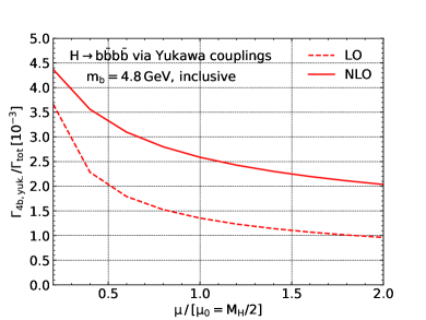
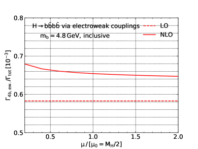
Figure 3: Decay branching ratio of the Higgs boson to four bottom quarks as a function of the renormalization scale via either Yukawa couplings (left plot) or the electroweak couplings (right plot), at both LO and NLO.

Full mass dependence of factors $\Delta_{ij}$ and $a_{ij}$ can be complicated. We provide their numerical values in Table. 1 for several choices of the bottom-quark pole mass. We set mass of the Higgs boson $M_{H}=125\,{\rm GeV}$, vacuum expectation value $v=246.22\,{\rm GeV}$, and $\alpha_{S}(M_{Z})=0.118$ in all numerical calculations. The from factors further depend on the masses of the electroweak gauge bosons, as well as their width, which we set to Tanabashi:2018oca

$$M_{W}=80.379\,{\rm GeV}, \qquad M_{Z}=90.1876\,{\rm GeV},$$

$$\Gamma_{Z}=2.4952\,{\rm GeV}, \qquad\Gamma_{W}=2.085\,{\rm GeV}.$$ (12)

Negative sign of $\Delta_{bg}$ shown in Table. 1 indicates a constructive interference between the Feynman diagrams due to bottom-quark Yukawa coupling and those induced by effective coupling with gluons. We found large NLO QCD corrections for $\Delta_{b\bar{b}}$, $\Delta_{gg}$, and the interference $\Delta_{bg}$ contributions, with mild dependence on the mass of the bottom quark. We further calculate the decay branching ratio of the four bottom quark channels assuming a total width of the Higgs boson $\Gamma_{tot}$ of 4 MeV 1101.0593 . We plot the decay branching ratio as a function of the renormalization scale in Fig. 3 at both LO and NLO for a bottom-quark mass of 4.8 GeV. The decay branching ratio due to Yukawa couplings can reach a few per mill and receives large QCD corrections. The LO prediction has a large scale uncertainty which is improved with the NLO corrections. The NLO prediction amounts to $2.59^{+0.7}_{-0.6}\times 10^{-3}$ if using a central scale of $\mu_{0}=M_{H}/2$ and a conventional scale variation by a factor of two. The decay branching ratio via electroweak couplings of the bottom quarks is smaller and receives mild QCD corrections. The NLO prediction is $0.656^{+0.01}_{-0.01}\times 10^{-3}$ using the same scale choice.

Figure 4: Fractional contributions to partial decay width of the Higgs boson to four bottom quarks as a function of the bottom quark mass, at both LO and NLO.

Fractional contributions from different terms to the total decay branching ratio to four bottom quarks are shown in Fig. 4 as a function of the bottom quark mass. Decay via electroweak couplings is sub-dominant but has larger contribution than interference of the bottom-quark Yukawa coupling and the gluon effective coupling. Decay due to pure gluon effective coupling is at the level of a few percents of the total decay branching ratio.

2.4 Jet cross sections

We consider final state with at least 4 $b$-tagged jets to separate from other multi-parton hadronic decay modes, for instance, Higgs boson decaying into a bottom quark pair plus two gluons or two light quarks. We use the $k_{T}$ jet algorithm Catani:1991hj with a resolution parameter $y$ varied between $10^{-3}$ and $0.5$. The separation of any two clusters are calculated as

$$d_{ij}=\frac{2\,{\rm min}(E_{i}^{2},E_{j}^{2})}{Q^{2}}(1-\cos\theta_{ij}),$$ (13)

with $Q^{2}=M_{H}^{2}/4$. Constituents of jets are combined with $E$ scheme by directly summing the four momentums. Flavor of jets are defined by counting net $b$-quark numbers within the jet, namely a jet with a $b$ quark and a $b$ anti-quark is considered as light-flavor jet 0704.2999 .

We show the decay branching ratio to 4 $b$-jets as a function of the jet resolution parameter in Fig. 5 via either Yukawa couplings or electroweak couplings with a bottom-quark mass of 4.8 GeV. In the upper panel we plot the branching ratio at LO and NLO. In the lower inset we show several ratios including the NLO prediction to the LO one for the nominal scale choice and the scale variations of the LO or NLO predictions. The jet rate approaches the inclusive rate of the decay when $y$ goes to 0 since then the four bottom quarks are always fully resolved. It decreases rapidly as the increasing of $y$ especially for the case of decay via Yukawa couplings where the dominant contributions are from quasi-collinear region of $b\bar{b}$ in the phase space. The effects of QCD corrections are similar as in the inclusive decay rate and exhibit mild dependence on the resolution parameter except when close to the endpoint region of the phase space. We found sizable NLO corrections and reduced scale variations for decay via Yukawa couplings. We further summarize the fractional contributions from different channels to the jet rate in Fig. 6. Contributions from $\Delta_{b\bar{b}}$ are always dominant while the contributions from $\Delta_{ZZ}$ increase with the increasing of the resolution parameter.

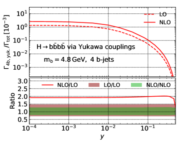
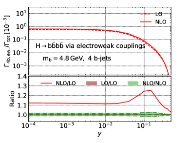
Figure 5: Decay branching ratio of the Higgs boson to four $b$-jets as a function of the jet resolution parameter via either Yukawa couplings (left plot) or the electroweak couplings (right plot), at both LO and NLO.

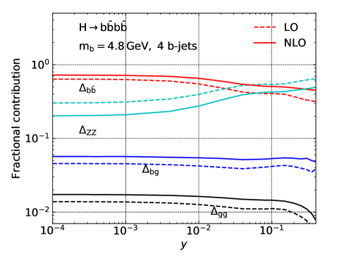
Figure 6: Fractional contributions to partial decay width of the Higgs boson to four $b$-jets as a function of the jet resolution parameter, at both LO and NLO.

2.5 Event topology

We consider several kinematic distributions of the final state $b$-jets, that includes energy of individual jets, invariant mass and energy of $b$-jet pairs. Jets are ordered according to their energies. For invariant mass of $b$-jet pairs, we include the highest and lowest mass among all combinations, $M_{bb,H}$, $M_{bb,L}$, the inclusive mass $M_{bb,inc}$ by counting all possible combinations, and the mass asymmetry $\Delta M_{bb}$ that is the minimum of absolute mass difference of two jet pairs for all possible divisions. We define similar variables for energy of jet pairs, highest and lowest pair energy $E_{bb,H}$ and $E_{bb,L}$, inclusive pair energy $E_{bb,inc}$, and the pair energy asymmetry $\Delta E_{bb}$. In case that the 4 $b$-jets arise from a cascade decay of two scalars with identical masses, the mass or energy asymmetry peaks at zero values.

We show representative results for a choice of the jet resolution parameter $y=0.02$ and $m_{b}=4.8$ GeV. That corresponds to an angular separation of $\Delta\theta\sim 0.3$ for two jets with the lower energy equals $M_{H}/4$. We first plot the energy distributions of each individual jet in Figs. 7-10. Energies are always normalized to the mass of the Higgs boson. We show the results for decay via Yukawa couplings and electroweak couplings in parallel with upper panel gives the differential decay branching ratio and lower inset gives ratio of NLO predictions to LO ones and their scale variations respectively. The distributions from two decay channels show clearly differences. For instance, the (sub-)leading jet peaks at slightly lower(higher) values for decay via electroweak couplings. The energy spectrum of the third and fourth jets are broader for decay via Yukawa couplings. Beside of the normalization, the QCD corrections induce changes on shape of the distributions. The spectrum is generally pushed to lower energy region due to the recoiled gluon in QCD real corrections, except for energy of the third and fourth jets in decay via electroweak couplings, where enhancements are found right after the peak region.

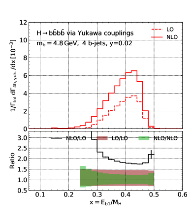
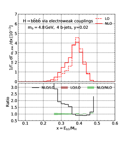
Figure 7: Differential decay branching ratio of the Higgs boson to four bottom quarks as a function of the energy of the leading $b$-jet, via the Yukawa couplings (left plot) and electroweak couplings (right plot), at both LO and NLO.

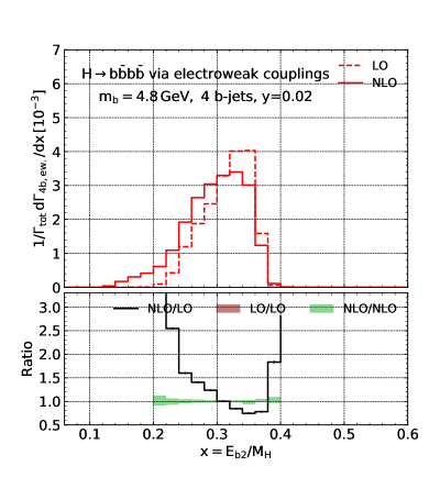
Figure 8: Similar to Fig. 7 for distribution as a function of of the energy of the sub-leading $b$-jet.

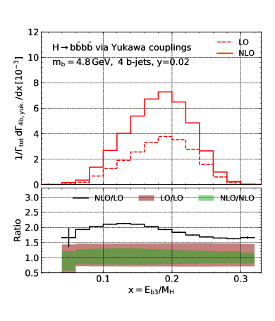
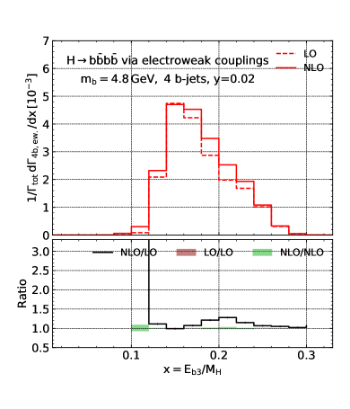
Figure 9: Similar to Fig. 7 for distribution as a function of of the energy of the third-leading $b$-jet.

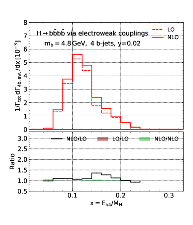
Figure 10: Similar to Fig. 7 for distribution as a function of of the energy of the softest $b$-jet.

We now move to distributions of invariant mass of jet pairs. In Fig. 11 we plot distribution of the highest invariant mass among all jet pairs in the event, $M_{b\bar{b},H}$. The decay via Yukawa couplings show a broad peak around 0.6$M_{H}$. On another hand decay via electroweak couplings has a narrow peak close to 0.7$M_{H}$ due to the dominant contributions from onshell $Z$ boson. Concerning shape of the distributions, the QCD corrections shift the spectrum to lower mass region for decay via Yukawa couplings. Both sides off the narrow peak are enhanced for decay via electroweak couplings because of the QCD real radiations. For the distribution of the lowest invariant mass $M_{b\bar{b},L}$ in Fig. 12, the decay via Yukawa couplings shows a sharp peak right after the mass threshold. In both decay channels the QCD corrections turn to induce a change of spectrum towards high mass regions. We plot the inclusive invariant mass distribution of jet pairs in Fig. 13. They show a much broader spectrum as expected and peak around 0.2$M_{H}$. The invariant mass peak at $Z$ boson mass in decay via electroweak couplings are diluted for the inclusive mass distribution. The QCD corrections sharpen the peak slightly in the case of decay via Yukawa couplings. Finally in Fig. 14 we show distributions of the invariant mass asymmetry. Both channels can have rather large asymmetry and show similar shapes. The QCD corrections are stable crossing the full kinematic range.

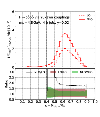
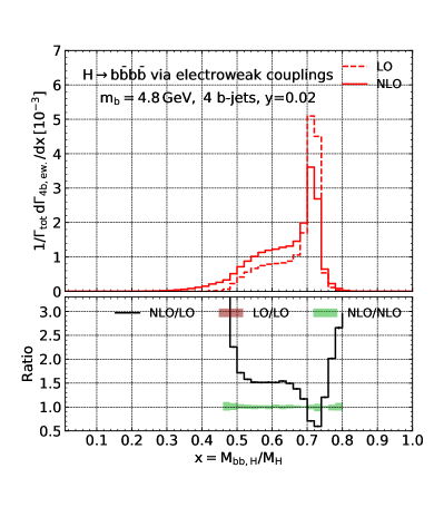
Figure 11: Similar to Fig. 7 for distribution as a function of of the highest invariant mass of all $b$-jet pairs.

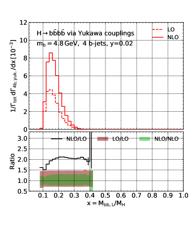
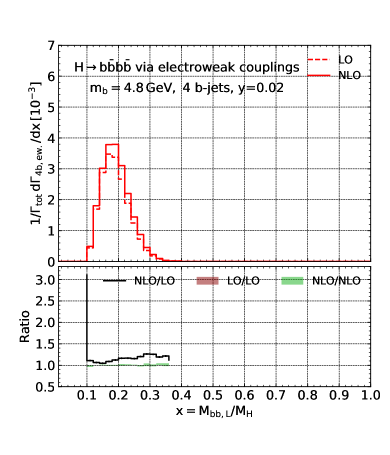
Figure 12: Similar to Fig. 7 for distribution as a function of the lowest invariant mass of all $b$-jet pairs.

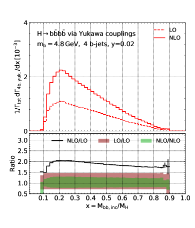
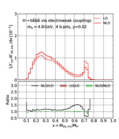
Figure 13: Similar to Fig. 7 for distribution as a function of the inclusive invariant mass of all $b$-jet pairs.

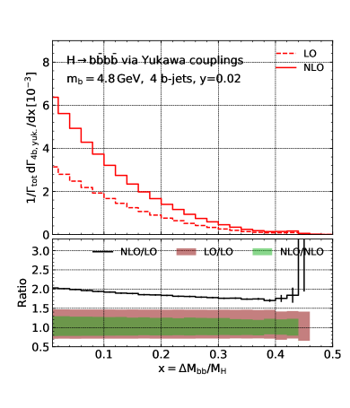
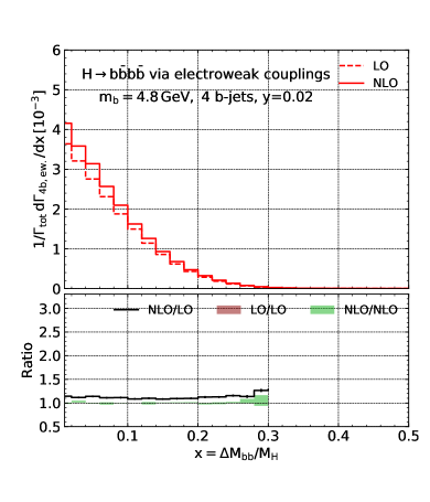
Figure 14: Similar to Fig. 7 for distribution as a function of the invariant mass asymmetry of all $b$-jet pairs.

We present various distributions on energy of the jet pairs in Figs. 15-18. The distribution on the highest energy of all jet pairs in Fig. 15 tends to be very similar to the case of highest invariant mass as discussed in Fig. 11 since they are mostly from the same jet pair. The impact of QCD corrections are also similar, namely push the spectrum to lower energy region for the decay through Yukawa couplings and broaden the $Z$ mass peak in the case of electroweak couplings. For the distribution on the lowest energy of all jet pairs in Fig. 16, at LO it is simply a reflection of the distribution on the highest energy of all jet pairs since the two energies add up to the Higgs boson mass. The QCD radiations change the shape of the distribution in a non-trivial way. Due to the same reason the inclusive energy distribution of all jet pairs in Fig. 17 are symmetric with respect to an energy of $M_{H}/2$ at LO. Thus the decay via electroweak couplings exhibits a triple-peak structure. For their shape the QCD corrections push the distribution to lower energy region in general due to energies carried away by gluon radiations. Energy of jet pairs can also show large asymmetry as presented in Fig. 18. The QCD corrections are almost constant for decay via Yukawa couplings and are largely enhanced towards the tail of the distribution for decay via electroweak couplings.

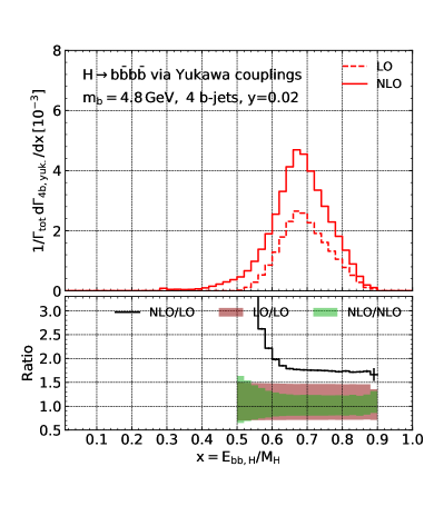
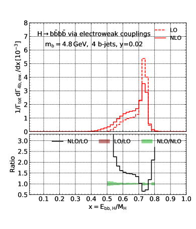
Figure 15: Similar to Fig. 7 for distribution as a function of the highest energy of all $b$-jet pairs.

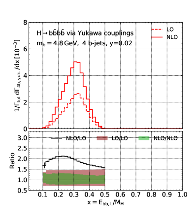
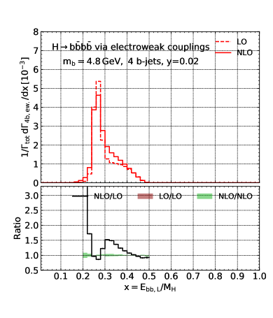
Figure 16: Similar to Fig. 7 for distribution as a function of the lowest energy of all $b$-jet pairs.

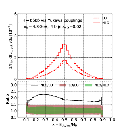
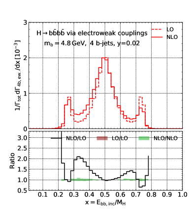
Figure 17: Similar to Fig. 7 for distribution as a function of the inclusive energy of all $b$-jet pairs.

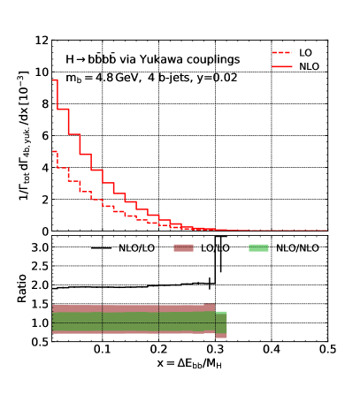
Figure 18: Similar to Fig. 7 for distribution as a function of the energy asymmetry of all $b$-jet pairs.

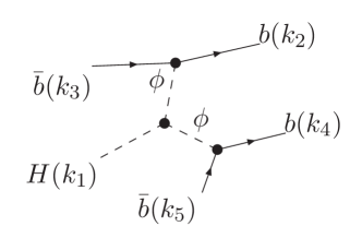
Figure 19: Feynman diagram at leading order for exotic decay of the Higgs boson to four bottom quarks via two light scalars.

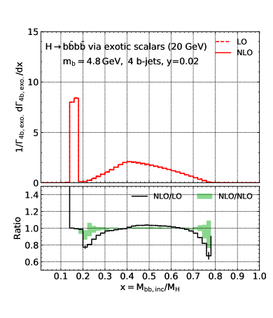
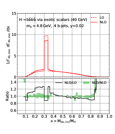
Figure 20: Normalized distribution of the Higgs boson decay to four bottom quarks as a function of the inclusive invariant mass of all $b$-jet pairs, via new light scalars with a mass of 20 GeV (left plot) and 40 GeV (right plot), at both LO and NLO.

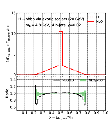
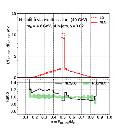
Figure 21: Similar to Fig. 20 for distribution as a function of the inclusive energy of all $b$-jet pairs.

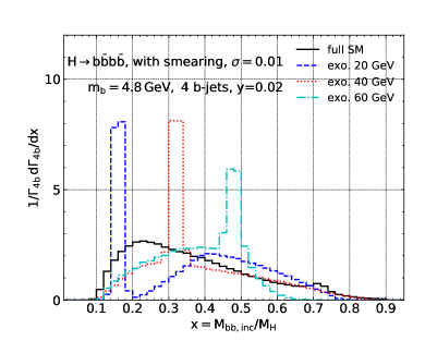
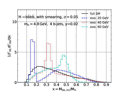
Figure 22: Comparison on normalized distribution of the Higgs boson decay to four bottom quarks as a function of the inclusive invariant mass of all $b$-jet pairs, for the SM decay and exotic decay via new light scalars with different masses, assuming an energy resolution of 1% (left plot) and 5% (right plot), at NLO in QCD.

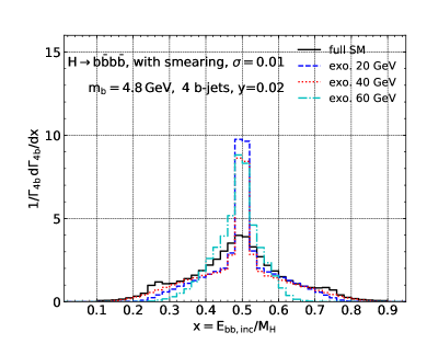
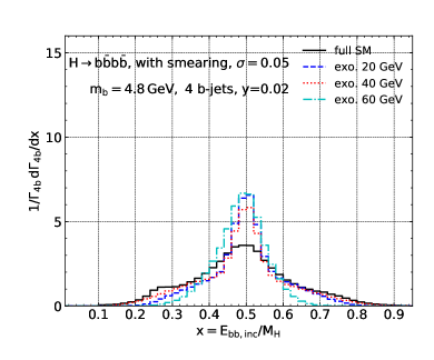
Figure 23: Similar to Fig. 22 for distribution as a function of the inclusive energy of all $b$-jet pairs.

3 Exotic decay

There have been proposals to study various exotic decay channels of the Higgs boson at both the LHC 1312.4992 and future electron-positron colliders Liu:2016zki . Higgs boson decays into four bottom quarks is among them and has been employed to search for possible new scalars with mass $\lesssim m_{H}/2$ at the LHC 1806.07355 , as demonstrated by Feynman diagram in Fig. 19. The ATLAS collaboration recently reported an upper limit of about 50% on the decay branching ratio of the Higgs boson to four bottom quarks via two light scalars 1806.07355 , depending on the mass and lifetime of the new scalar. In this section we first investigate the QCD corrections to this exotic decay channel as we did for the SM case. Afterwards we compare various kinematic distributions for Higgs boson decays into four bottom quarks via two light scalars to those predicted in the SM.

3.1 Kinematic distributions and QCD corrections

In the calculation of the exotic decay, we assume the light scalar to be CP-even similar to the SM Higgs boson. We renormalize the Yukawa coupling between the bottom quark and the new scalar with the $\overline{\rm MS}$ scheme. We also assume the new scalar has a small width thus the narrow width approximation can be applied. We are mostly interested in two kinematic distributions, i.e., the inclusive invariant mass distribution and the inclusive energy distribution of $b$-jet pairs. They are relevant for the exotic decay via new scalars which will show up either as a sharp peak at the scalar mass or a sharp peak at half of the Higgs mass respectively. We plot the normalized distribution of $M_{b\bar{b},inc}$ in Fig. 20 for a scalar mass of 20 and 40 GeV. We compare the shape at LO and NLO. For a lower mass of the new scalar, the QCD corrections barely modify the shape except for the tail regions. We observe a slightly broader peak with the QCD corrections for a larger scalar mass. The impact of QCD corrections are similar for $E_{b\bar{b},inc}$ shown in Fig. 21.

3.2 Comparison to the SM case

For a future electron-positron collider, for instance, CEPC, the Higgs boson can be produced abundantly and collected with a high efficiency. With a center of mass energy of 250 GeV and an integrated luminosity of 5.6 ab^-1, we expect a total number of the Higgs boson of about $1.1\times 10^{6}$ in $ZH$ production. Thus in the SM it predicts a total of about 4000 events for the Higgs boson decaying into four bottom quarks based on the decay branching ratio in Sect. 2. Such a rate can be measured with a precision of 2% if taking into account only statistical uncertainties and assuming perfect background rejection. The SM decay of course contributes as an important background for searches of the exotic decay via two new scalars, not mentioning other non-resonant processes, e.g., $e^{+}e^{-}\rightarrow Zb\bar{b}b\bar{b}$. In Fig. 22 we compare the normalized distribution of $M_{b\bar{b},inc}$ for the decay to four bottom quarks in the SM and via the new scalars at NLO in QCD. The SM result includes both decays via Yukawa couplings and electroweak couplings. We consider new scalars with a mass of 20, 40 and 60 GeV respectively. We further apply a Gaussian smearing on the distributions since the signal over background ratio strongly depends on the detector energy resolution. In the left and right plots we assume an energy resolution of 1% and 5% respectively. One can see clearly distortions of the signal peak while the background is less modified. In Fig. 23 we present similar comparison for normalized distribution of $E_{b\bar{b},inc}$. Impact of the energy smearing are similar as shown in Fig. 22. The inclusive energy of $b$-jet pairs show less discrimination power as comparing to the inclusive invariant mass of $b$-jet pairs especially after taking into account the realistic jet energy resolution.

4 Conclusions

We study in details decays of the standard model Higgs boson to two bottom quark and anti-quark pairs. The hadronic decay can be triggered either by Yukawa couplings of bottom and top quarks or the electroweak couplings. Both channels are calculated to next-to-leading order in QCD with the former one utilizing effective theory with top quarks integrated out. We found large NLO QCD corrections for decay via Yukawa couplings that lead to a 90% increase of the inclusive partial decay width and residual QCD scale variations of about 20%. On another hand we found moderate NLO QCD corrections of about 12% for inclusive partial decay width of decay via electroweak couplings. We also calculated various jet cross sections and kinematic distributions. The QCD corrections can result in significant changes not only on normalizations but also on shape of various distributions. At future Higgs factory, all hadronic decay channels of the Higgs boson including the one to four bottom quarks can be explored and measured. Especially they can be employed to directly search for new physics beyond the standard model, e.g., possible new light scalars that can induce exotic decay of the Higgs boson to four bottom quarks. Thus we further compare predictions on various kinematic distributions of the decay in the SM and induced by those new scalars. To complete the study on searches for new physics in the four bottom quark decay channel it will be desirable to carry out a refined study with all SM backgrounds included, e.g., those from non-Higgs boson production processes, and with realistic detector coverage and resolution included. Further matching of the NLO calculations with parton showering and QCD hadronizations will also be required. We leave those topics for a future study.

References

- (1) G. Aad et al. [ATLAS Collaboration], Phys. Lett. B 716 (2012) 1 doi:10.1016/j.physletb.2012.08.020 [arXiv:1207.7214 [hep-ex]].
- (2) S. Chatrchyan et al. [CMS Collaboration], Phys. Lett. B 716 (2012) 30 doi:10.1016/j.physletb.2012.08.021 [arXiv:1207.7235 [hep-ex]].
- (3) A. M. Sirunyan et al. [CMS Collaboration], Phys. Rev. Lett. 120 (2018) no.23, 231801 doi:10.1103/PhysRevLett.120.231801 [arXiv:1804.02610 [hep-ex]].
- (4) M. Aaboud et al. [ATLAS Collaboration], Phys. Lett. B 784 (2018) 173 doi:10.1016/j.physletb.2018.07.035 [arXiv:1806.00425 [hep-ex]].
- (5) M. Aaboud et al. [ATLAS Collaboration], Phys. Lett. B 786 (2018) 59 doi:10.1016/j.physletb.2018.09.013 [arXiv:1808.08238 [hep-ex]].
- (6) A. M. Sirunyan et al. [CMS Collaboration], Phys. Rev. Lett. 121 (2018) no.12, 121801 doi:10.1103/PhysRevLett.121.121801 [arXiv:1808.08242 [hep-ex]].
- (7) S. Heinemeyer et al. [LHC Higgs Cross Section Working Group], doi:10.5170/CERN-2013-004 arXiv:1307.1347 [hep-ph].
- (8) T. Behnke et al., arXiv:1306.6327 [physics.acc-ph].
- (9) J. Guimaraes da Costa et al. [CEPC Study Group], arXiv:1811.10545 [hep-ex].
- (10) P. Lebrun et al., doi:10.5170/CERN-2012-005 arXiv:1209.2543 [physics.ins-det].
- (11) M. Bicer et al. [TLEP Design Study Working Group], JHEP 1401 (2014) 164 doi:10.1007/JHEP01(2014)164 [arXiv:1308.6176 [hep-ex]].
- (12) J. L. Abelleira Fernandez et al. [LHeC Study Group], J. Phys. G 39 (2012) 075001 doi:10.1088/0954-3899/39/7/075001 [arXiv:1206.2913 [physics.acc-ph]].
- (13) M. Klein, doi:10.1142/9789813238053_0015 arXiv:1802.04317 [hep-ph].
- (14) F. An et al., Chin. Phys. C 43 (2019) no.4, 043002 doi:10.1088/1674-1137/43/4/043002 [arXiv:1810.09037 [hep-ex]].
- (15) C. Anastasiou, C. Duhr, F. Dulat, F. Herzog and B. Mistlberger, Phys. Rev. Lett. 114 (2015) 212001 doi:10.1103/PhysRevLett.114.212001 [arXiv:1503.06056 [hep-ph]].
- (16) B. Mistlberger, JHEP 1805 (2018) 028 doi:10.1007/JHEP05(2018)028 [arXiv:1802.00833 [hep-ph]].
- (17) F. A. Dreyer and A. Karlberg, Phys. Rev. Lett. 117 (2016) no.7, 072001 doi:10.1103/PhysRevLett.117.072001 [arXiv:1606.00840 [hep-ph]].
- (18) R. Boughezal, F. Caola, K. Melnikov, F. Petriello and M. Schulze, JHEP 1306 (2013) 072 doi:10.1007/JHEP06(2013)072 [arXiv:1302.6216 [hep-ph]].
- (19) X. Chen, T. Gehrmann, E. W. N. Glover and M. Jaquier, Phys. Lett. B 740 (2015) 147 doi:10.1016/j.physletb.2014.11.021 [arXiv:1408.5325 [hep-ph]].
- (20) R. Boughezal, F. Caola, K. Melnikov, F. Petriello and M. Schulze, Phys. Rev. Lett. 115 (2015) no.8, 082003 doi:10.1103/PhysRevLett.115.082003 [arXiv:1504.07922 [hep-ph]].
- (21) R. Boughezal, C. Focke, W. Giele, X. Liu and F. Petriello, Phys. Lett. B 748 (2015) 5 doi:10.1016/j.physletb.2015.06.055 [arXiv:1505.03893 [hep-ph]].
- (22) S. Borowka, N. Greiner, G. Heinrich, S. P. Jones, M. Kerner, J. Schlenk and T. Zirke, JHEP 1610 (2016) 107 doi:10.1007/JHEP10(2016)107 [arXiv:1608.04798 [hep-ph]].
- (23) Y. Gong, Z. Li, X. Xu, L. L. Yang and X. Zhao, Phys. Rev. D 95 (2017) no.9, 093003 doi:10.1103/PhysRevD.95.093003 [arXiv:1609.03955 [hep-ph]].
- (24) Q. F. Sun, F. Feng, Y. Jia and W. L. Sang, Phys. Rev. D 96 (2017) no.5, 051301 doi:10.1103/PhysRevD.96.051301 [arXiv:1609.03995 [hep-ph]].
- (25) W. Chen, F. Feng, Y. Jia and W. L. Sang, Chin. Phys. C 43 (2019) no.1, 013108 doi:10.1088/1674-1137/43/1/013108 [arXiv:1811.05453 [hep-ph]].
- (26) P. A. Baikov, K. G. Chetyrkin and J. H. Kuhn, Phys. Rev. Lett. 96 (2006) 012003 doi:10.1103/PhysRevLett.96.012003 [hep-ph/0511063].
- (27) J. Davies, M. Steinhauser and D. Wellmann, Nucl. Phys. B 920, 20 (2017) doi:10.1016/j.nuclphysb.2017.04.012 [arXiv:1703.02988 [hep-ph]].
- (28) F. Herzog, B. Ruijl, T. Ueda, J. A. M. Vermaseren and A. Vogt, JHEP 1708, 113 (2017) doi:10.1007/JHEP08(2017)113 [arXiv:1707.01044 [hep-ph]].
- (29) P. A. Baikov and K. G. Chetyrkin, Phys. Rev. Lett. 97 (2006) 061803 doi:10.1103/PhysRevLett.97.061803 [hep-ph/0604194].
- (30) A. Denner, S. Heinemeyer, I. Puljak, D. Rebuzzi and M. Spira, Eur. Phys. J. C 71 (2011) 1753 doi:10.1140/epjc/s10052-011-1753-8 [arXiv:1107.5909 [hep-ph]].
- (31) M. Spira, Prog. Part. Nucl. Phys. 95 (2017) 98 doi:10.1016/j.ppnp.2017.04.001 [arXiv:1612.07651 [hep-ph]].
- (32) C. Anastasiou, F. Herzog and A. Lazopoulos, JHEP 1203 (2012) 035 doi:10.1007/JHEP03(2012)035 [arXiv:1110.2368 [hep-ph]].
- (33) V. Del Duca, C. Duhr, G. Somogyi, F. Tramontano and Z. Trócsányi, JHEP 1504 (2015) 036 doi:10.1007/JHEP04(2015)036 [arXiv:1501.07226 [hep-ph]].
- (34) R. Mondini, M. Schiavi and C. Williams, arXiv:1904.08960 [hep-ph].
- (35) W. Bernreuther, L. Chen and Z. G. Si, JHEP 1807 (2018) 159 doi:10.1007/JHEP07(2018)159 [arXiv:1805.06658 [hep-ph]].
- (36) D. E. Kaplan and M. McEvoy, Phys. Lett. B 701 (2011) 70 doi:10.1016/j.physletb.2011.05.026 [arXiv:0909.1521 [hep-ph]].
- (37) D. Curtin et al., Phys. Rev. D 90 (2014) no.7, 075004 doi:10.1103/PhysRevD.90.075004 [arXiv:1312.4992 [hep-ph]].
- (38) Z. Liu, L. T. Wang and H. Zhang, Chin. Phys. C 41 (2017) no.6, 063102 doi:10.1088/1674-1137/41/6/063102 [arXiv:1612.09284 [hep-ph]].
- (39) S. Liu, Y. L. Tang, C. Zhang and S. h. Zhu, Eur. Phys. J. C 77, no. 7, 457 (2017) doi:10.1140/epjc/s10052-017-5012-5 [arXiv:1608.08458 [hep-ph]].
- (40) M. Aaboud et al. [ATLAS Collaboration], JHEP 1810 (2018) 031 doi:10.1007/JHEP10(2018)031 [arXiv:1806.07355 [hep-ex]].
- (41) A. Bredenstein, A. Denner, S. Dittmaier and M. M. Weber, Phys. Rev. D 74 (2006) 013004 doi:10.1103/PhysRevD.74.013004 [hep-ph/0604011].
- (42) A. Bredenstein, A. Denner, S. Dittmaier and M. M. Weber, JHEP 0702 (2007) 080 doi:10.1088/1126-6708/2007/02/080 [hep-ph/0611234].
- (43) G. Li, Z. Li, Y. Liu, Y. Wang and X. Zhao, Phys. Rev. D 98 (2018) no.7, 076010 doi:10.1103/PhysRevD.98.076010 [arXiv:1805.10138 [hep-ph]].
- (44) J. Gao, Y. Gong, W. L. Ju and L. L. Yang, JHEP 1903 (2019) 030 doi:10.1007/JHEP03(2019)030 [arXiv:1901.02253 [hep-ph]].
- (45) M. X. Luo, V. Shtabovenko, T. Z. Yang and H. X. Zhu, arXiv:1903.07277 [hep-ph].
- (46) J. Gao, JHEP 1801 (2018) 038 doi:10.1007/JHEP01(2018)038 [arXiv:1608.01746 [hep-ph]].
- (47) R. Mondini and C. Williams, arXiv:1904.08961 [hep-ph].
- (48) J. C. Collins, F. Wilczek and A. Zee, Phys. Rev. D 18 (1978) 242. doi:10.1103/PhysRevD.18.242
- (49) K. G. Chetyrkin, J. H. Kuhn and M. Steinhauser, Comput. Phys. Commun. 133 (2000) 43 doi:10.1016/S0010-4655(00)00155-7 [hep-ph/0004189].
- (50) A. L. Kataev, N. V. Krasnikov and A. A. Pivovarov, Nucl. Phys. B 198 (1982) 508 Erratum: [Nucl. Phys. B 490 (1997) 505] doi:10.1016/0550-3213(82)90338-8, 10.1016/S0550-3213(97)00101-6 [hep-ph/9612326].
- (51) T. Inami, T. Kubota and Y. Okada, Z. Phys. C 18 (1983) 69. doi:10.1007/BF01571710
- (52) S. Dawson, Nucl. Phys. B 359 (1991) 283. doi:10.1016/0550-3213(91)90061-2
- (53) A. Djouadi, M. Spira and P. M. Zerwas, Phys. Lett. B 264 (1991) 440. doi:10.1016/0370-2693(91)90375-Z
- (54) A. L. Kataev and V. T. Kim, Mod. Phys. Lett. A 9 (1994) 1309. doi:10.1142/S0217732394001131
- (55) L. R. Surguladze, Phys. Lett. B 341 (1994) 60 doi:10.1016/0370-2693(94)01253-9 [hep-ph/9405325].
- (56) M. Spira, A. Djouadi, D. Graudenz and P. M. Zerwas, Nucl. Phys. B 453 (1995) 17 doi:10.1016/0550-3213(95)00379-7 [hep-ph/9504378].
- (57) K. G. Chetyrkin, B. A. Kniehl and M. Steinhauser, Nucl. Phys. B 510 (1998) 61 doi:10.1016/S0550-3213(98)81004-3, 10.1016/S0550-3213(97)00649-4 [hep-ph/9708255].
- (58) G. Cullen et al., Eur. Phys. J. C 74 (2014) no.8, 3001 doi:10.1140/epjc/s10052-014-3001-5 [arXiv:1404.7096 [hep-ph]].
- (59) P. Mastrolia, E. Mirabella and T. Peraro, JHEP 1206 (2012) 095 Erratum: [JHEP 1211 (2012) 128] doi:10.1007/JHEP11(2012)128, 10.1007/JHEP06(2012)095 [arXiv:1203.0291 [hep-ph]].
- (60) T. Peraro, Comput. Phys. Commun. 185 (2014) 2771 doi:10.1016/j.cpc.2014.06.017 [arXiv:1403.1229 [hep-ph]].
- (61) A. van Hameren, C. G. Papadopoulos and R. Pittau, JHEP 0909 (2009) 106 doi:10.1088/1126-6708/2009/09/106 [arXiv:0903.4665 [hep-ph]].
- (62) A. van Hameren, Comput. Phys. Commun. 182 (2011) 2427 doi:10.1016/j.cpc.2011.06.011 [arXiv:1007.4716 [hep-ph]].
- (63) S. Catani, S. Dittmaier, M. H. Seymour and Z. Trocsanyi, Nucl. Phys. B 627 (2002) 189 doi:10.1016/S0550-3213(02)00098-6 [hep-ph/0201036].
- (64) A. Denner, S. Dittmaier, M. Roth and L. H. Wieders, Nucl. Phys. B 724 (2005) 247 Erratum: [Nucl. Phys. B 854 (2012) 504] doi:10.1016/j.nuclphysb.2011.09.001, 10.1016/j.nuclphysb.2005.06.033 [hep-ph/0505042].
- (65) J. Alwall et al., JHEP 1407 (2014) 079 doi:10.1007/JHEP07(2014)079 [arXiv:1405.0301 [hep-ph]].
- (66) A. Djouadi, Phys. Rept. 457 (2008) 1 doi:10.1016/j.physrep.2007.10.004 [hep-ph/0503172].
- (67) M. Tanabashi et al. [Particle Data Group], Phys. Rev. D 98 (2018) no.3, 030001. doi:10.1103/PhysRevD.98.030001
- (68) S. Dittmaier et al. [LHC Higgs Cross Section Working Group], doi:10.5170/CERN-2011-002 arXiv:1101.0593 [hep-ph].
- (69) S. Catani, Y. L. Dokshitzer, M. Olsson, G. Turnock and B. R. Webber, Phys. Lett. B 269 (1991) 432. doi:10.1016/0370-2693(91)90196-W
- (70) A. Banfi, G. P. Salam and G. Zanderighi, JHEP 0707 (2007) 026 doi:10.1088/1126-6708/2007/07/026 [arXiv:0704.2999 [hep-ph]].