Dynamic Routing Networks

Abstract

The deployment of deep neural networks in real-world applications is mostly restricted by their high inference costs. Extensive efforts have been made to improve the accuracy with expert-designed or algorithm-searched architectures. However, the incremental improvement is typically achieved with increasingly more expensive models that only a small portion of input instances really need. Inference with a static architecture that processes all input instances via the same transformation would thus incur unnecessary computational costs. Therefore, customizing the model capacity in an instance-aware manner is much needed for higher inference efficiency. In this paper, we propose Dynamic Routing Networks (DRNets), which support efficient instance-aware inference by routing the input instance to only necessary transformation branches selected from a candidate set of branches for each connection between transformation nodes. The branch selection is dynamically determined via the corresponding branch importance weights, which are first generated from lightweight hypernetworks (RouterNets) and then recalibrated with Gumbel-Softmax before the selection. Extensive experiments show that DRNets can reduce a substantial amount of parameter size and FLOPs during inference with prediction performance comparable to state-of-the-art architectures.

1 Introduction

Deep convolutional neural networks (CNNs) [8, 42] have revolutionized computer vision with increasingly large and sophisticated architectures. The architectures are typically designed and tuned by domain experts with rich engineering experience. These models achieve remarkable performance with hundreds of layers and millions of parameters, which however consume a substantial amount of computational resources during inference. Improving inference efficiency has thus become a major issue for the deployment of deep neural networks in real-world applications.

Recently, there has been a growing body of research on efficient network design [11, 28, 33] for more efficient inference architectures. These works mainly focus on designing more efficient transformations to reduce the parameter size and inference FLOPs. Many architectures with efficient transformation building blocks have been proposed. Particularly, SqueezeNet [15] reduces the parameter size significantly with the squeeze-and-expand convolution block. MobileNets [11] substantially reduce the parameter size and computation cost measured in FLOPs on mobile devices with depthwise separable convolution. Subsequent works such as MobileNetV2 [28] and ShuffleNetV2 [22] further reduce FLOPs on the target hardware. However, it is well recognized that designing these architectures is a non-trivial task that requires engineering expertise.

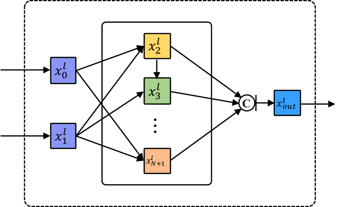
(a) Cell Structure

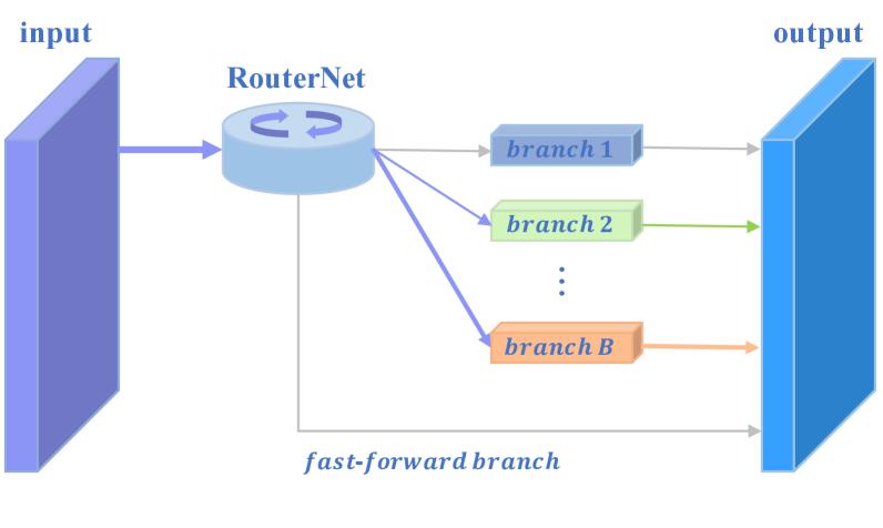
(b) Node Connection

Figure 1: Left: the Cell structure of DRNets with inter-connected nodes. Right: the illustration of a node connection with $B$+1 transformation branches. During inference, each input instance is routed to only necessary branches for efficiency. Importance weights of branches are dynamically generated from the RouterNet and then recalibrated with Gumbel-Softmax.

To automate the architecture design process, there has been an increasing interest in Neural Architecture Search (NAS). Mainstream NAS algorithms [41, 42, 26] search for the network architecture iteratively. In each iteration, an architecture is proposed by the search algorithm and then trained and evaluated. The evaluation performance is in turn utilized to update the algorithm. This process is incredibly slow because both the algorithm and the proposed architectures require extensive training. In particular, the reinforcement learning (RL) based algorithm NASNet [42] takes 1800 GPU days, and the evolution based algorithm AmoebaNet [26] costs 3150 GPU days to obtain the final architecture. To expedite the search process, many acceleration methods [1, 19, 2, 25] have been proposed. Many recent works [20, 39, 4, 36] instead remove the search algorithm and instead optimize parameters of both the architecture and the selection process concurrently with gradient-based algorithms. Among these methods, the gradient-based NAS algorithms turn out to be both efficient and effective for the architecture search.

By and large, expert-designed and NAS-searched models are quite efficient and accurate during inference. Nonetheless, most architectures of these models are static during inference, and thus not adaptive to the varying complexity of input instances. In real-world applications, only a small portion of input instances require deep representations [33, 13], as made evident by the diminishing marginal returns of increasing model size on accuracy. Therefore, extensive computational resources could be wasted if all input instances are processed in the same way. To further improve the inference efficiency over existing architectures, designing a dynamic architecture with adequate representational power to support the inference of hard instances, and meanwhile a flexible mechanism to provide only necessary computation for instances of varying difficulty is thus much needed.

To support dynamic inference, we propose DRNets to support instance-aware inference with the building block Cell and the transformation of the node connection illustrated in Figure 1. At a high level, DRNets can be regarded as a dynamic architecture generator with its backbone network building upon best-performing expert-designed and NAS-searched architectures, which produce architectures customized for the current input instance for higher inference efficiency. Specifically, the backbone network is a stack of $L$ structurally identical Cells. Each cell contains $N$ inter-connected Nodes and receives inputs from the outputs of its two preceding cells. Instead of painstakingly searching for the connection topology and the respective transformation for each node connection of the cell as in NAS [41, 42, 26, 20], each node of DRNets is simply connected to a predetermined subset of its previous node(s), e.g., two in Figure 1(a), and each connection transforms the current instance via a candidate operation set of $B$+1 transformation branches. These $B$ branches can be homogeneous or heterogeneous, which are trained to specialize in certain types of instances. There is another fast-forward branch integrated to efficiently forward the current instance without heavy computation.

To enable instance-aware architecture customization, we integrate $L$ lightweight hypernetworks RouterNets, one for each cell to dynamically determine the relative importance weight of each branch among the $B$+1 branches of each connection. We further introduce Gumbel-Softmax [16, 23] to recalibrate the importance weights of each connection so that during training, these weights are dense and the entire architecture is efficiently optimized, and during inference, the input instance is routed only to necessary branches of larger importance weights for efficiency as illustrated in Figure 1(b). The advantages of DRNets can be summarized as follows:

• The architecture of DRNets is general and customizable, which supports the instance-aware dynamic routing mechanism and thus improves inference efficiency significantly by reducing redundant computation.

• DRNets introduce Gumbel-Softmax to lightweight RouterNets during the branch selection process, which enables direct gradient descent optimization and is more tractable than the RL-based methods.

• DRNets achieve state-of-the-art inference efficiency in terms of parameter size and FLOPs and inherently supports applications that require runtime control.

Our experiments show that DRNets are extremely efficient during inference which selects only necessary branches on a per-input basis. For instance, DRNets reduce the parameter size by 3.71x and FLOPs by 4.53x respectively compared with the NAS-searched high-performance architecture DARTS [20] on CIFAR-10 with comparable accuracy. With a tiny model of 0.57M parameters, DRNets achieve much better accuracy while with only 13.48% parameter size and 46.41% FLOPs during inference compared with the expert-designed network MobileNetV2 1.5x [28]. We also provide ablation studies and visualize the branch selection process to better understand the proposed dynamic routing mechanism.

The remainder of this paper is organized as follows: we first discuss the related works in Section 2. Then in section 3, we introduce the backbone network and the hypernetworks of DRNets in detail. Experimental evaluations of DRNets are provided in Section 4, where the main results and findings are summarized in Section 4.2 and Section 4.3. Finally, Section 5 concludes the paper.

2 Related Work

Efficient Architecture Design. An increasing number of works focus on directly designing resource-aware networks [15, 22, 11, 28]. SqueezeNet [15] proposes the fire module of the squeeze-and-expand convolution, which reduces the parameter size substantially. MobileNets [11, 28, 10] series architectures adopt depthwise separable convolution for efficient inference. MobileNetV2 [28] achieves higher efficiency with inverted residual blocks, and MobileNetV3 [10] further improves efficiency with the integration of components searched by NAS. ShuffleNet [40] introduces the lightweight channel shuffle operation for information exchange between channel groups, and ShuffleNetV2 [22] further improve inference speed by considering the actual overhead on the target platform. To provide efficient inference, many of these transformations are adopted in the candidate operation set of DRNets.

Neural Architecture Search. There has been an increasing interest in automated architecture search (NAS). Given the learning task, NAS aims to find the optimal architecture, specifically, the topology of network connections between nodes and the transformation operation for each connection. NAS typically consists of two stages, i.e., architecture optimization and parameter optimization. Mainstream NAS methods [42, 26] consider architecture optimization as a stand-alone process that is separated from the parameter optimization. Search algorithms, such as RL-based NAS [41, 42] and evolutionary-based NAS [37, 26], obtain high-performing architectures while at the cost of an unprecedented amount of search time. Many works have been proposed to expedite the search process, e.g., via performance prediction [1, 19], hyperparameter generating initialization weights [3], weight sharing [25], and etc.

Many recent works [4, 36] instead integrate the architecture search and architecture optimization into one gradient-based optimization framework. In particular, DARTS [20] relaxes the discrete search space to continuous operation mixing weights for each connection and optimizes the weights directly with gradient back-propagated from the validation loss. Likewise, SNAS [39] models the discrete search space with sets of one-hot random variables, which are made differentiable by sampling from continuous Concrete Distribution [16, 23]. DRNets also relax the discrete branch selection to continuous importance weights that are optimized by gradient descent. While instead of obtaining a set of fixed weights, RouterNets are introduced to dynamically generate these weights to support instance-aware architecture customization for efficiency.

Dynamic Inference Architecture. A growing body of research has been investigating methods to accelerate inference, e.g., model compression via weight pruning [7], vector quantization, knowledge distillation [9] and etc. Typically, these methods are designed as post-training techniques. Relatively fewer works explore dynamic inference architectures, which supports instance-aware execution. The dynamic inference is based on the observation that most input instances can be accurately processed with a small network, and only a few inputs need an expensive model.

The idea of dynamic inference is related to mixture-of-experts [29], whereas in DRNets, the input is dynamically routed to specialized branches instead of individual models. Most prior dynamic inference architectures [29, 27, 18] focus mainly on accuracy, and their architectures are introduced in abstract terms. To improve efficiency, the two ResNet [8] based architectures SkipNet [33] and AIG [32] propose to dynamically skip each residual layer. While the backbone network of DRNets adopts the topology and efficient branches of best-performing architectures [28, 20], which provides more efficient and diversified branch selection for higher efficiency. Further, the dynamic skipping of SkipNet [33] and AIG [32] are based on a hypernetwork trained with policy gradient [34] and straight-through Gumbel-Softmax [16] respectively. However, training with policy gradient is brittle and often stuck in poor optima; the Straight-Through gradient estimation of AIG is biased [32, 16, 23] and easily falls into the selection collapse of sampling only a few branches repeatedly. Compared with SkipNet and AIG, the hypernetworks of DRNets are optimized more effectively with a two-stage temperature annealing scheme, and DRNets support a varied branch selection of multiple branches for each connection instead of the binary skipping choice. MSDNet [13] inserts multiple classifiers into a multi-scale version of DenseNet [14] and supports faster predictions by exiting into a classifier. DRNets can also selectively route the input to lightweight branches for accelerating predictions.

3 Dynamic Routing Network

We aim to devise an efficient and flexible backbone network for DRNet so that during inference, accompanying hypernetworks can dynamically produce a customized architecture for each input instance for higher inference efficiency. We introduce the backbone network in Section 3.1, hypernetworks in Section 3.2, and the optimization and efficient inference in Section 3.3.

3.1 The Backbone Network

Following NAS [41, 20, 39], the backbone of DRNet is constructed with a stack of $L$ Cells. As illustrated in Figure 1(a), each cell is a directed acyclic graph consisting of an ordered sequence of $N$ intermediate nodes, which receives inputs $x_{0}^{l}$ and $x_{1}^{l}$ from outputs of the two preceding cells. Each intermediate node $x_{i}^{l}(i>1)$ of the $l_{th}$ cell learns latent representations and receives inputs from a set of $n$ previous nodes of smaller indexes $I_{i}^{l}$, e.g., $n=2$ in Figure 1(a):

$$x_{i}^{l}=\sum_{j\in I_{i}^{l}}\mathcal{F}_{j,i}(x_{j}^{l}),j<i\wedge|I_{i}^{l}|=n$$ (1)

The main task of NAS is to find the best cell connection topology given by $I_{i}^{l}$, i.e., best previous nodes (two nodes for most NAS architectures [41, 20, 39]) for each intermediate node, and meanwhile, determine the best branch from candidates for each node connection. We sidestep the architecture search by using a hypernetwork, which will be introduced in Section 3.2, to dynamically determine the necessary branches for each connection given the current input instance for higher efficiency.

Thereby, there are $C=n\cdot N$ connections for each cell. As is illustrated in Figure 1(b), the connection passes information from node $x_{j}^{l}$ to $x_{i}^{l}$ via a predetermined set of $B$+1 candidate transformation branches, e.g., operations adopted from efficient networks [28, 40] and NAS [20, 39]:

$$\mathcal{F}_{j,i}(x_{j}^{l})=\sum_{b=0}^{B}w_{b}\cdot\mathcal{F}_{b}(x_{j}^{l})=\sum_{b=0}^{B}w_{b}\cdot(\mathcal{W}_{b}\ast x_{j}^{l})$$ (2)

where $\mathcal{W}_{b}$ is the transformation weights (e.g., the weight matrix of a linear layer or a convolutional kernel), $\ast$ denotes the transformation (e.g., matrix multiplication or a convolutional operation), and $w_{b}$ indicates and importance of the $b_{th}$ branch. The branch importance weight $w_{b}$ is dynamically determined by the cell hypernetwork (RouterNet^l), rather than a fixed learned parameter as in most NAS methods [20, 39]. For each connection, the $B$+1 importance weights are recalibrated with Gumbel-Softmax so that these branches can be effectively trained and specialized for different input instances during training; while during inference, only the most important branches are selected for prediction efficiency. We will elaborate on RouterNet and Gumbel-Softmax in Section 3.2.

The candidate operation set should contain at least one fast-forward branch, e.g., identity mapping, to minimize unnecessary computation for easy instances. Further, the training cost of Equation 2 can be greatly reduced by preparing the aggregate transformation weights before the computation-heavy input transformation, with the reformulation: $\sum_{b=0}^{B}w_{b}\cdot(\mathcal{W}_{b}\ast x_{j}^{l})=(\sum_{b=0}^{B}w_{b}\cdot\mathcal{W}_{b})\ast x_{j}^{l}$. Finally, the output of the cell $x_{out}^{l}$ is collected by concatenating outputs from all intermediate nodes $\{x_{2}^{l},\dots,x_{N+1}^{l}\}$. We shall use superscript $l$, subscript $c$ and $b$ to index the cell, connection, and branch respectively.

Recent works [38] demonstrate that architectures with randomly generated connections achieve surprisingly competitive results compared with the best-performing NAS models, which is also confirmed in our experiments. In this paper, we thus adopt a simple connection topology introduced in Section 4.1 and focus mainly on the branch selection mechanism and the impact of dynamic routing on inference efficiency. With such a dynamic architecture, we can readily adjust the candidate operation set for each connection to customize the model capacity and inference efficiency based on the task difficulty and resource constraints in deployment.

3.2 Dynamic Weight Recalibration with RouterNet

To support instance-aware inference control, we introduce one lightweight hypernetwork RouterNet for each cell. Each $\textit{RouterNet}^{l}$ receives the same input as the $l_{th}$ cell, specifically, the output nodes $x_{out}^{l-2},x_{out}^{l-1}$ ($x_{0}^{l},x_{1}^{l}$) from the two preceding cells, and generates importance weights $\boldsymbol{W}^{l}$ for the $C$ connections of the corresponding cell at once:

$$\boldsymbol{W}^{l}=\textit{RouterNet}^{l}(x_{0}^{l},x_{1}^{l}),\boldsymbol{W}^{l}\in\mathbb{R}^{C\times(B+1)}$$ (3)

Specifically, each $\textit{RouterNet}^{l}$ weighs each branch of the connection with the respective importance weight during training; and further, as illustrated in Figure 1(b), routes the current input to only necessary branches during inference. In this work, the RouterNet comprises a pipeline of 2 convolutional blocks, a global average pooling, and finally an affine transformation to produce the weights. The convolution block adopts the separable convolution [28], specifically a point-wise convolution and a depth-wise convolution of stride two and kernel size 5$\times$5. The convolution block with large stride and kernel size incurs minimal computational overhead while extracts necessary features for the generation of the importance weights.

The importance weights are introduced along the lines of convolutional attention mechanism [24, 12, 35], where attention weights are first determined based on the input instance and then used to recalibrate the activations of certain input dimensions, e.g., channels [12]. In DRNets, the importance weights are applied to transformation branches of each connection, where each candidate branch is coupled with a respective weight for branch selection.

The Gumbel-Softmax [16, 23] and reparameterization technique [17] are integrated to recalibrate the importance weights generated by RouterNets. The weight recalibration is a continuous relaxation of the categorical branch sampling process, which enables tractable gradient-based optimization for the entire network during training. Specifically, $\widetilde{w}_{c,b}^{l}$ (the importance weight of $b_{th}$ branch of the $c_{th}$ connection in the $l_{th}$ cell) after the recalibration of ${w}_{c,b}^{l}$ ($\boldsymbol{W}_{c}^{l}\in\mathbb{R}^{B+1}$) with Gumbel-Softmax follows a Concrete Distribution [23]:

$$\widetilde{w}_{c,b}^{l}=\frac{\exp((w_{c,b}^{l}+g_{c,b}^{l})/\tau)}{\sum_{b^{\prime}=0}^{B}\exp((w_{c,b^{\prime}}^{l}+g_{c,b^{\prime}}^{l})/\tau)},\tau>0$$ (4)

where $\tau$ is the temperature of the softmax and is annealed steadily during training, and $g_{c,b}^{l}$=$-\log(-\log(u_{c,b}^{l}))$ is a $Gumbel(0,1)$ [23] random variable for the $b_{th}$ branch by sampling $u_{c,b}^{l}$ from Uniform Distribution $\mathcal{U}(0,1)$ [16]. $\widetilde{w}_{c,b}^{l}$ is then directly used for branch weighting in Equation 2. Denoting parameters of the backbone network and RouterNets as $\theta$ and $\phi$, then the objective function $\mathcal{L}_{CE}(\theta,\phi)$ can be reparameterized as:

$$\mathcal{L}_{CE}(\theta,\phi) =\mathbb{E}_{\widetilde{w}\sim p_{\phi}(\mathbf{x})}[f_{\theta}(\mathbf{x},\widetilde{w})]$$ (5)

$$=\mathbb{E}_{g\sim Gumbel(0,1)}[f_{\theta}(\mathbf{x},h_{\phi}(\mathbf{x},g))]$$

where $\mathbf{x}$ is the current input instance and the dependence of the importance weights $\widetilde{w}$ on the parameters of $\phi$ can be transferred from the sampling of $p_{\phi}(\mathbf{x})$ into $h_{\phi}(\mathbf{x},g)$. With such reparameterization, the branch selection weights $\widetilde{w}_{c,b}^{l}$ can be computed as a deterministic function of the weights $w_{c,b}^{l}$ generated from RouterNets with parameters $\phi$ and an independent random variable $u_{c,b}^{l}$, such that non-differentiable categorical branch sampling process is made directly differentiable with respect to $\phi$ during training. The weight $\widetilde{w}_{c,b}^{l}$ following Concrete Distribution [23] satisfies the nice properties: (1) $\widetilde{w}_{c,b}=\frac{1}{B+1},\tau\rightarrow+\infty$, and (2)

$$p(\lim_{\tau\rightarrow 0}\widetilde{w}_{c,b}^{l}=1)=\exp(w_{c,b}^{l})/\sum_{b^{\prime}=0}^{B}\exp(w_{c,b^{\prime}}^{l})$$ (6)

which indicates that the softmax computation of Equation 4 smoothly approaches discrete argmax branch selection as the temperature $\tau$ anneals. High temperature leads to uniform dense branch selection, while a lower temperature tends to select the most important branch following a Categorical Distribution parameterized by $softmax(\boldsymbol{W}_{c}^{l})$.

3.3 Optimization and Efficient Inference

With the continuous relaxation of the Gumbel-Softmax (Equation 4) and reparameterization (Equation 5), the branch selection process of the RouterNets is made directly differentiable with respect to the parameters of RouterNets using the chain rule:

$$\nabla_{\phi}\mathcal{L}_{CE}(\theta,\phi) =\mathbb{E}_{g}[\nabla_{\phi}f_{\theta}(\mathbf{x},h_{\phi}(\mathbf{x},g))]$$ (7)

$$=\mathbb{E}_{g}[f^{\prime}_{\theta}(\mathbf{x},h_{\phi}(\mathbf{x},g))\nabla_{\phi}h_{\phi}(\mathbf{x},g)]$$

where the gradient $\frac{\partial\mathcal{L}}{\partial\widetilde{w}_{c,b}^{l}}$ backpropagated from the loss function $\mathcal{L}_{CE}$ to $\widetilde{w}_{c,b}^{l}$ through the backbone network via $f^{\prime}_{\theta}(\mathbf{x},h_{\phi}(\mathbf{x},g))$ can be directly backpropagated to $w_{c,b}^{l}$ with low variance [23], and further to the $RouterNet^{l}$ via $\nabla_{\phi}h_{\phi}(\mathbf{x},g)$ unimpededly. Therefore, parameters of the entire DRNet can be optimized in an end-to-end manner by gradient descent effectively.

During training, the temperature $\tau$ of Equation 4 regulates the sparsity of the branch selection. A relatively higher temperature forces the weights to distribute more uniformly so that all the branches can be efficiently trained. While a low temperature instead tends to sparsely sample one branch from the categorical distribution parameterized by the importance weights dynamically determined by RouterNets, and thus supports efficient inference by routing inputs to only necessary branches. We thus propose a two-stage training scheme for DRNets: (1) the first stage pretrains the entire network with a fixed relatively high temperature till convergence. (2) the second stage fine-tunes the parameters with $\tau$ steadily annealing to a low temperature. The first stage ensures that all the branches are sufficiently trained and specialized for certain input instances; the fine-tuning and annealing in the second stage help maintain the performance of DRNets with dynamic routing during inference for higher efficiency.

To further improve inference efficiency, a regularization term is explicitly introduced during the fine-tuning stage, which takes into account the expectation of the resource consumption $\mathcal{R}$ in the final loss function $\mathcal{L}$ for the already correctly-classified input instances:

$$\mathcal{L} =\mathcal{L}_{CE}+\lambda\mathds{1}_{\mathrm{\hat{\mathbf{y}}=\mathbf{y}}}\log\mathbb{E}[\mathcal{R}]$$ (8)

$$\approx\mathcal{L}_{CE}+\lambda\mathds{1}_{\mathrm{\hat{\mathbf{y}}=\mathbf{y}}}\log\sum_{l=1}^{L}\sum_{c=1}^{C}\sum_{b=0}^{B}\widetilde{w}_{c,b}^{l}\cdot\mathcal{R}(\mathcal{F}_{c,b}^{l}(\cdot))$$

where $\mathcal{L}_{CE}$ denotes the cross-entropy loss (Equation 5), $\mathbf{y}$ is the ground truth class label, $\hat{\mathbf{y}}$ is the prediction, $\lambda$ controls the regularization strength and $\mathcal{R}(\cdot)$ calculates the resource consumption of each branch $\mathcal{F}_{c,b}^{l}(\cdot)$. The branch importance weight $\widetilde{w}_{c,b}^{l}$ represents the probability of the corresponding transformation $\mathcal{F}_{c,b}^{l}(\cdot)$ being selected during inference, and thus the regularization term $\mathbb{E}[\mathcal{R}]$ corresponds to the expectation of the computational resource required for each input instance. The resource regularizer can be adapted based on deployment constraints, which may include the parameter size, FLOPs, and memory access cost (MAC), and etc. In this paper, we mainly focus on the inference time measured by FLOPs, where $\mathcal{R}(\mathcal{F}_{c,b}^{l}(\cdot))$ is a constant and can be calculated beforehand. This indicates that the regularizer $\mathcal{R}$ is also directly differentiable with respect to $\widetilde{w}_{c,b}^{l}$ during the optimization. We denote DRNets trained with regularization strength $\lambda$ as DRNet-R-$\lambda$.

As illustrated in Figure 1(b), during inference, dynamic routing for efficiency is achieved by passing the input to the top-$k$ most important branches out of the $B$+1 branches for each connection, whose overall importance weights denoted as $s_{c}^{l}$ just exceeds a predetermined threshold $T$. After the selection, the recalibration weight $\widetilde{w}_{c,b}^{l}$ of the selected branch is rescaled by $\frac{1}{s_{c}^{l}}$ to stabilize the scale of the connection output. Consequently, each RouterNet selects only necessary branches for each instance depending on the input difficulty and the computational cost of each branch to trade off between $\mathcal{L}_{CE}$ and $\mathcal{R}$. In this paper, the same threshold is shared among all connections for simplicity, and DRNets inference with a threshold $t$ is denoted as DRNet-T-t.

Under such an inference scheme, the backbone network comprises up to $(2^{B+1}-1)^{L\cdot C}$ possible candidate subnets, corresponding to each unique branch selection of all $L\cdot C$ connections. For a small 10 cells DRNet, with 8 connections per cell and 5 candidate operations per connection, there are ${(2^{5}-1)^{8\cdot 10}}\approx 2\cdot 10^{119}$ possible candidate architectures of different branch selections, which is orders of magnitudes larger than the search space of conventional NAS [25, 20, 39, 4, 31].

4 Experiments

We mainly focus on the evaluation of the accuracy and efficiency of DRNets on benchmark datasets. We compare the results of DRNets against the best-performing expert-designed, NAS-searched and dynamic inference architectures. Experimental details are provided in Section 4.1, and main results are reported in Section 4.2. We discuss and visualize the dynamic routing process in Section 4.3.

4.1 Experimental Setup

Dataset. Following conventions [39, 20], we report the performance of DRNets on benchmark datasets CIFAR-10 and ImageNet-12, where the accuracy and inference efficiency are compared with other state-of-the-art architectures. CIFAR-10 contains 50,000 training images and 10,000 test images of $32\times 32$ pixels in 10 classes. We adopt standard data pre-processing and augmentation pipeline [20, 39] and apply AutoAugment [5], cutout [6] of length 16. ImageNet contains 1.2 million training and 50,000 validation images in 1000 classes. We adopt a standard augmentation scheme following [20, 39] and apply label smoothing of 0.1 and AutoAugment. Results are reported with a $224\times 224$ center crop.

Temperature Annealing Scheme. In the pre-training stage, the temperature $\tau$ is fixed to 3 till convergence. In the fine-tuning stage, $\tau$ is reset to 1.0 and is further annealed by $\exp(-0.0006)\approx 0.999$ every epoch to 0.5. The initial $\tau$ is 5 and exponentially annealed to 0.8 for ImageNet.

Candidate Operation Set. The following 5 candidate operations ($B$+1=5) are adopted for demonstration, which can be readily adjusted in deployment:

• $3\times 3$ max-pooling

• $3\times 3$ avg-pooling

• skip connection

• $3\times 3$ separable-conv

• $5\times 5$ separable-conv

In particular, skip connection is adopted as the fast-forward branch that allows for efficient input forwarding; pooling layers contain no parameter and are computationally lightweight; separable-conv dominates the parameter size and computation in each connection, which contains separable convolutions of ReLU-Conv-Conv-BN. The three types of transformations support trade-offs between model capacity and efficiency for the branch selection of each connection.

Architecture Details We adopt three DRNet architectures of different size: (1) DRNet(S), a smaller network with $L$=5 cells and 15 initial channels; (2) DRNet(M), a medium network with 10 cells and 20 initial channels; (3) DRNet(L), a larger network with 10 cells and 32 initial channels.

All the architectures adopt $N$=$4$ intermediate nodes for each cell and a plain node connection strategy where each node is connected to $n$=$2$ preceding nodes, specifically $x_{i-1}^{l}$ and randomly $x_{0}^{l}$ or $x_{1}^{l}$ for simplicity. Further, nodes directly connected to input nodes are downsampled with stride 2 for the $\frac{L}{3}$-th and $\frac{2L}{3}$-th cells. An auxiliary classifier with weight 0.4 is connected to the output of the $\frac{2L}{3}$-th cell for additional regularization.

Optimization Details. Following conventions [20, 39, 30], we apply SGD with Nesterov-momentum 0.9 and weight decay $3\cdot 10^{-5}$ for 250 epochs of 0.97 learning rate decay for ImageNet. For CIFAR-10, we apply SGD with momentum 0.9 and weight decay $3\cdot 10^{-4}$ for 1200 epochs for both training stages. The learning rate is initialized to 0.025 and 0.005 for the pre-training and fine-tuning stage respectively. The batch size is set to 128 to fit the entire DRNet into one NVIDIA Titan RTX. We adopt higher structural level dropout for better regularization during training, specifically, drop-connection linearly increased to 0.1, and drop-branch to 0.7 for CIFAR-10. The learning rate is annealed to zero with the cosine learning rate scheduler [21].

4.2 Performance Evaluation

Overall Results and Discussion.

Architecture	Test Error	Params	FLOPs	Search Method	Search Space	Search Cost
	(%)	(M)	(M)			(GPU days)
ResNet-110 [8]	6.43	1.73	255.3	manual	–	–
DenseNet-L190-k40 [14]	3.46	25.6	9345	manual	–	–
ShuffleNetV2 1.5$\times$ [22]$\dagger$	6.36	2.49	95.70	manual	–	–
MobileNetV2 1.0$\times$ [28]$\dagger$	5.56	2.30	94.42	manual	–	–
NASNet-A [42]$\dagger$	2.65	3.3	505.1	RL	cell	1800
AmoebaNet-A [26]$\dagger$	3.12	3.1	514.9	evolution	cell	3150
ENAS [25]$\dagger$	2.83	4.7	767.8	RL	cell	2.2
DARTS [20]	3.00	3.3	542.0	gradient	cell	1.9
ConvNet-AIG-110 [32]	5.76	1.78	410	gradient	layer-wise	–
SkipNet-110-HRL [33]	6.70	1.75	150.6	RL	layer-wise	–
MSDNet [13]$\dagger$	6.82	5.44	54.35	manual	–	–
DRNet(S)-R-0.1-T-0.8	3.66 / 4.21	0.57 / 0.31	84.65 / 43.82	gradient	layer-wise	–
DRNet(M)-R-0.1-T-0.8	2.84 / 3.44	1.86 / 0.89	267.3 / 119.6	gradient	layer-wise	–
DRNet(L)-R-0.1-T-0.8	2.27 / 2.84	4.41 / 2.16	603.1 / 265.8	gradient	layer-wise	–

Table 1: Performance (Inference with All Branches/Dynamic Routing) of DRNets compared with representative expert-designed, NAS-searched and dynamic inference architectures on CIFAR-10. Results marked with $\dagger$ are obtained by training respective architectures with our implementation.

Table 1 summarizes the overall performance of DRNets on CIFAR-10. In terms of total training cost, DRNets take only 2.5 and 5.5 GPU training days for DRNet(S) and DRNet(M) respectively without explicit architecture search. The training time of DRNet is up to three orders of magnitudes less than evolution-based NAS or RL-based NAS, thanks to the efficient end-to-end gradient-based optimization scheme.

Architecture	Test Error	Params	FLOPs
	(%)	(M)	(M)
1.0 MobileNet [11]	29.4	4.2	569
ShuffleNet $2\times$ [40]	29.1	5.0	524
NASNet0-A [42]	26.0	5.3	564
DARTS [20]	26.9	4.9	595
ConvNet-AIG-50-t-0.4 [32]	24.8	26.56	2560
SkipNet-101 [33]	27.9	26.56	2147
DRNet(L)-R-0.01-T-0.8	29.8	3.8	351

Table 2: Inference performance of DRNet(L) compared with representative expert-designed, NAS-searched and dynamic inference architectures on ImageNet.

For inference performance, DRNets with dynamic routing considerably reduce the parameter size and FLOPs compared with baseline networks. In particular, DRNet(S)-R-0.1-T-0.8 takes 0.31M parameters and 43.82M FLOPs on average during inference, specifically, only 13.48% and 46.41% of efficient network MobileNetV2 $1.0\times$ [28] with 1.35% higher accuracy; DRNet(M)-R-0.1-T-0.8 achieves up to 3.71x and 4.53x parameter size and FLOPs reduction compared with DARTS [20], with a minor 0.44% accuracy decrease; further, DRNet(L)-R-0.1-T-0.9 achieves accuracy comparable to the best NAS-searched architectures (2.27% with all branches and 2.84% with dynamic routing) while takes only 265.8M Flops, which is around half of their inference FLOPs. Compared with other dynamic inference networks, in particular, SkipNet-110-HRL [33] that dynamically determines to skip each residual layer with an RL-trained hypernetwork, and MSDNet [13] that supports inference time accuracy-efficiency trade-offs by giving predictions with intermediate features, DRNet(S)-R-0.1-T-0.8 achieves a notably lower test error rate of 4.21% and meanwhile much more efficient inference with only 43.82M FLOPs on average.

We note that such a significant reduction in prediction parameter size and FLOPs can be ascribed to the adoption of efficient operations following MobileNets and NAS, and the fact that not all instances need an expensive architecture to be correctly classified. Therefore, dynamic routing inputs to only necessary branches can reduce redundant computation considerably.

Architecture	Test Error	Params	FLOPs
	(%)	(M)	(M)
DRNet(S)-w/o-RouterNet	4.78	0.46	77.34
DRNet(S)-Softmax	4.37	0.57	84.65
$\hookrightarrow$ DRNet(S)-Softmax-T-0.8	5.27 (+0.90%)	0.55 (-3.51%)	80.99 (-4.32%)
DRNet(S)-Gumbel-Softmax	3.66	0.57	84.65
$\hookrightarrow$ DRNet(S)-R-0.0-T-0.8	4.07 (+0.41%)	0.33 (-42.1%)	47.91 (-43.4%)
$\hookrightarrow$ DRNet(S)-R-0.1-T-0.8	4.21 (+0.55%)	0.31 (-45.6%)	43.82 (-48.2%)
$\hookrightarrow$ DRNet(S)-R-0.5-T-0.8	5.85 (+2.19%)	0.20 (-64.9%)	29.28 (-65.4%)

Table 3: Inference performance of DRNet(S) with different regularization strengths. The amount of reduction compared with the respective full networks is given in parentheses.

Table 2 reports the performance of representative architectures and DRNets with a thresholds of 0.8 on ImageNet. The results show that DRNet(L) obtains competitive prediction performance compared with expert-designed architectures and lower accuracy than NAS-searched architectures. The lower accuracy can be largely attributed to the simple connection topology adopted in the backbone of DRNet, as we focus on showing the effectiveness of the proposed dynamic routing mechanism in reducing unnecessary computation instead of obtaining state-of-the-art accuracy.

With the dynamic routing of RouterNet, one single model of DRNet supports accuracy-efficiency trade-offs by simply controlling the importance threshold $T$ during inference. In particular, DRNet(L) inference with a threshold 0.8 reduces FLOPs by 27.63% with a minor accuracy decrease, and can further reduce FLOPs with a lower threshold. These results show that DRNets can also support applications that require runtime accuracy-efficiency control.

Ablation studies. We further examine the effect of the hypernetworks RouterNets and regularization strength quantitatively in Table 3. We train DRNets without hypernetworks (DRNet(S)-w/o-RouterNet), which increases test error by 1.12% from 3.66% to 4.78% as compared with DRNets trained with Gumbel-Softmax (DRNet(S)-Gumbel-Softmax). We also find that DRNets trained with Gumbel-Softmax obtain noticeably lower test error compared with DRNets train with Softmax only (DRNet(S)-Softmax). Further, DRNet(S)-Softmax only reduces a very limited amount of 4.32% FLOPs with dynamic routing inference. These findings suggest that RouterNet and the Gumbel-Softmax recalibration are essential to obtain high accuracy and efficiency during inference. Specifically, RouterNets enable instance-aware branch selection, and Gumbel-Softmax makes the selection process optimizable during training and efficient during inference. We also train DRNet(S) with different regularization strengths. Results show that a larger regularization strength effectively trades off prediction accuracy for higher efficiency. E.g., with a regularization strength 0.5, DRNets-R-0.5-T-0.8 only takes 29.28M inference FLOPs, a reduction of 65.4% FLOPs, while the test error increases by 1.78% compared with the full network DRNet(S)-Gumbel-Softmax.

4.3 Visualization of Dynamic Routing

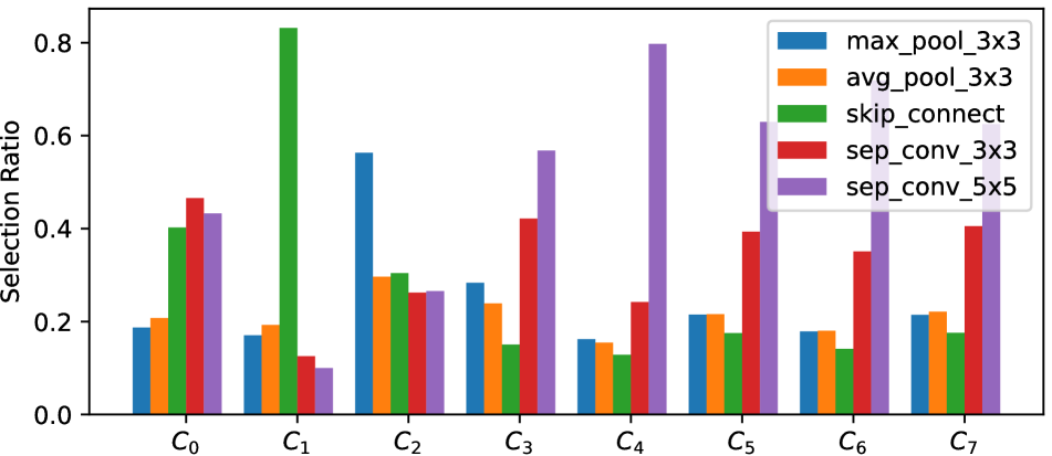
Figure 2: Branch selection ratio for each connection with dynamic routing during inference in a representative cell of DRNet(S)-R-0.1-T-0.8 on CIFAR-10.

Branch Selection Ratio. We visualize in Figure 2 the average branch selection ratio of one representative cell of DRNet(S)-R-0.1-T-0.8 with dynamic routing, which shows the ratio of each branch being selected by RouterNets during inference. Figure 2 confirms that the transformations required for different input instances vary greatly. In particular, lightweight pooling and skip connection branches are commonly selected, and thus, a considerable amount of computation can be saved.

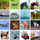
(a) Easy Instances

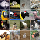
(b) Hard Instances

Figure 3: Visualization of easy and hard instances of model DRNet(M)-R-0.1-T-0.8 on CIFAR-10. Easy instances are generally clearer and brighter, while hard instances are darker and blurry.

Qualitative Difference between Instances. Denoting instances that the network is confident with in prediction as easy instance and uncertain about as hard instance, we can then show the cluster of easy and hard instances in Figure 3 to help understand the dynamic routing mechanism. We find that in DRNets, the confidence of the prediction is highly correlated to the image quality. Specifically, easy instances are more salient (clear with high contrast) while hard instances are more inconspicuous (dark with low contrast). We then compute the accuracy and average FLOPs of these two types of instances. Easy instances achieve higher classification accuracy with 23.1% fewer FLOPs on average compared to hard instances. This suggests that although instances from the same dataset are generally regarded as i.i.d., the prediction difficulty of different instances still differs greatly, and thus a sizeable amount of computation can be reduced by dynamically cutting off unnecessary branches for relatively easier instances.

5 Conclusion

In this paper, we present DRNets, a general architecture framework that supports input-aware inference by dynamic routing. Lightweight hypernetwork RouterNets are integrated to dynamically produce customized architectures for different instances so that inputs can be dynamically routed to only necessary branches for efficiency. We also introduce Gumbel-Softmax and the reparameterization trick to the routing process, which enables tractable and effective gradient-based training, and more importantly, extremely efficient inference. The inference efficiency is enhanced with the resource-aware regularization. Experimental results with ablation studies and visualizations confirm the efficiency of the dynamic routing architecture.

References

- [1] Bowen Baker, Otkrist Gupta, Ramesh Raskar, and Nikhil Naik. Accelerating neural architecture search using performance prediction. In 6th International Conference on Learning Representations, ICLR, 2018.
- [2] Gabriel Bender, Pieter-Jan Kindermans, Barret Zoph, Vijay Vasudevan, and Quoc Le. Understanding and simplifying one-shot architecture search. In International Conference on Machine Learning, 2018.
- [3] Andrew Brock, Theodore Lim, James M. Ritchie, and Nick Weston. SMASH: one-shot model architecture search through hypernetworks. In 6th International Conference on Learning Representations, ICLR 2018, Vancouver, BC, Canada, April 30 - May 3, 2018, Conference Track Proceedings, 2018.
- [4] Han Cai, Ligeng Zhu, and Song Han. Proxylessnas: Direct neural architecture search on target task and hardware. In 7nd International Conference on Learning Representations, ICLR, 2019.
- [5] Ekin D Cubuk, Barret Zoph, Dandelion Mane, Vijay Vasudevan, and Quoc V Le. Autoaugment: Learning augmentation policies from data. arXiv preprint arXiv:1805.09501, 2018.
- [6] Terrance DeVries and Graham W Taylor. Improved regularization of convolutional neural networks with cutout. arXiv preprint arXiv:1708.04552, 2017.
- [7] Song Han, Jeff Pool, John Tran, and William J. Dally. Learning both weights and connections for efficient neural network. In Advances in Neural Information Processing Systems 28: Annual Conference on Neural Information Processing Systems 2015, December 7-12, 2015, Montreal, Quebec, Canada, pages 1135–1143, 2015.
- [8] Kaiming He, Xiangyu Zhang, Shaoqing Ren, and Jian Sun. Deep residual learning for image recognition. In Proceedings of the IEEE conference on computer vision and pattern recognition, pages 770–778, 2016.
- [9] Geoffrey E. Hinton, Oriol Vinyals, and Jeffrey Dean. Distilling the knowledge in a neural network. CoRR, abs/1503.02531, 2015.
- [10] Andrew Howard, Mark Sandler, Grace Chu, Liang-Chieh Chen, Bo Chen, Mingxing Tan, Weijun Wang, Yukun Zhu, Ruoming Pang, Vijay Vasudevan, Quoc V. Le, and Hartwig Adam. Searching for mobilenetv3. ICCV, 2019.
- [11] Andrew G Howard, Menglong Zhu, Bo Chen, Dmitry Kalenichenko, Weijun Wang, Tobias Weyand, Marco Andreetto, and Hartwig Adam. MobileNets: efficient convolutional neural networks for mobile vision applications. CoRR, abs/1704.04861, 2017.
- [12] Jie Hu, Li Shen, and Gang Sun. Squeeze-and-excitation networks. In Proceedings of the IEEE conference on computer vision and pattern recognition, pages 7132–7141, 2018.
- [13] Gao Huang, Danlu Chen, Tianhong Li, Felix Wu, Laurens van der Maaten, and Kilian Q Weinberger. Multi-scale dense networks for resource efficient image classification. In 6th International Conference on Learning Representations, ICLR, 2018.
- [14] Gao Huang, Zhuang Liu, Laurens Van Der Maaten, and Kilian Q Weinberger. Densely connected convolutional networks. In Proceedings of the IEEE conference on computer vision and pattern recognition, pages 4700–4708, 2017.
- [15] Forrest N. Iandola, Matthew W. Moskewicz, Khalid Ashraf, Song Han, William J. Dally, and Kurt Keutzer. Squeezenet: Alexnet-level accuracy with 50x fewer parameters and <1mb model size. ICLR, 2017.
- [16] Eric Jang, Shixiang Gu, and Ben Poole. Categorical reparameterization with gumbel-softmax. In 5th International Conference on Learning Representations, ICLR, 2017.
- [17] Diederik P. Kingma and Max Welling. Auto-encoding variational bayes. In 2nd International Conference on Learning Representations, ICLR 2014, Banff, AB, Canada, April 14-16, 2014, Conference Track Proceedings, 2014.
- [18] Louis Kirsch, Julius Kunze, and David Barber. Modular networks: Learning to decompose neural computation. In Advances in Neural Information Processing Systems 31: Annual Conference on Neural Information Processing Systems 2018, NeurIPS, pages 2414–2423, 2018.
- [19] Chenxi Liu, Barret Zoph, Maxim Neumann, Jonathon Shlens, Wei Hua, Li-Jia Li, Li Fei-Fei, Alan Yuille, Jonathan Huang, and Kevin Murphy. Progressive neural architecture search. In Proceedings of the European Conference on Computer Vision (ECCV), 2018.
- [20] Hanxiao Liu, Karen Simonyan, and Yiming Yang. DARTS: differentiable architecture search. In 7th International Conference on Learning Representations, ICLR, 2019.
- [21] Ilya Loshchilov and Frank Hutter. SGDR: stochastic gradient descent with warm restarts. In 5th International Conference on Learning Representations, ICLR 2017, Toulon, France, April 24-26, 2017, Conference Track Proceedings, 2017.
- [22] Ningning Ma, Xiangyu Zhang, Hai-Tao Zheng, and Jian Sun. Shufflenet v2: Practical guidelines for efficient cnn architecture design. In Proceedings of the European Conference on Computer Vision (ECCV), 2018.
- [23] Chris J. Maddison, Andriy Mnih, and Yee Whye Teh. The concrete distribution: A continuous relaxation of discrete random variables. In 5th International Conference on Learning Representations, ICLR, 2017.
- [24] Alejandro Newell, Kaiyu Yang, and Jia Deng. Stacked hourglass networks for human pose estimation. In Computer Vision - ECCV 2016 - 14th European Conference, Amsterdam, The Netherlands, October 11-14, 2016, Proceedings, Part VIII, pages 483–499, 2016.
- [25] Hieu Pham, Melody Y Guan, Barret Zoph, Quoc V Le, and Jeff Dean. Efficient neural architecture search via parameter sharing. In Proceedings of the 35th International Conference on Machine Learning, ICML, 2018.
- [26] Esteban Real, Alok Aggarwal, Yanping Huang, and Quoc V Le. Regularized evolution for image classifier architecture search. In Proceedings of the AAAI conference on artificial intelligence, volume 33, pages 4780–4789, 2019.
- [27] Clemens Rosenbaum, Tim Klinger, and Matthew Riemer. Routing networks: Adaptive selection of non-linear functions for multi-task learning. In 6th International Conference on Learning Representations, ICLR, 2018.
- [28] Mark Sandler, Andrew Howard, Menglong Zhu, Andrey Zhmoginov, and Liang-Chieh Chen. Mobilenetv2: Inverted residuals and linear bottlenecks. In Proceedings of the IEEE Conference on Computer Vision and Pattern Recognition, pages 4510–4520, 2018.
- [29] Noam Shazeer, Azalia Mirhoseini, Krzysztof Maziarz, Andy Davis, Quoc V. Le, Geoffrey E. Hinton, and Jeff Dean. Outrageously large neural networks: The sparsely-gated mixture-of-experts layer. In 5th International Conference on Learning Representations, ICLR, 2017.
- [30] Yao Shu, Wei Wang, and Shaofeng Cai. Understanding architectures learnt by cell-based neural architecture search. In 8th International Conference on Learning Representations, ICLR, 2020.
- [31] Dimitrios Stamoulis, Ruizhou Ding, Di Wang, Dimitrios Lymberopoulos, Bodhi Priyantha, Jie Liu, and Diana Marculescu. Single-path nas: Designing hardware-efficient convnets in less than 4 hours. arXiv preprint arXiv:1904.02877, 2019.
- [32] Andreas Veit and Serge J. Belongie. Convolutional networks with adaptive inference graphs. In Computer Vision - ECCV, pages 3–18. Springer, 2018.
- [33] Xin Wang, Fisher Yu, Zi-Yi Dou, Trevor Darrell, and Joseph E Gonzalez. Skipnet: Learning dynamic routing in convolutional networks. In Proceedings of the European Conference on Computer Vision (ECCV), pages 409–424, 2018.
- [34] Ronald J. Williams. Simple statistical gradient-following algorithms for connectionist reinforcement learning. Machine Learning, 8:229–256, 1992.
- [35] Sanghyun Woo, Jongchan Park, Joon-Young Lee, and In So Kweon. Cbam: Convolutional block attention module. In Proceedings of the European Conference on Computer Vision (ECCV), pages 3–19, 2018.
- [36] Bichen Wu, Xiaoliang Dai, Peizhao Zhang, Yanghan Wang, Fei Sun, Yiming Wu, Yuandong Tian, Peter Vajda, Yangqing Jia, and Kurt Keutzer. Fbnet: Hardware-aware efficient convnet design via differentiable neural architecture search. In IEEE Conference on Computer Vision and Pattern Recognition, CVPR 2019, Long Beach, CA, USA, June 16-20, 2019, pages 10734–10742, 2019.
- [37] Lingxi Xie and Alan L. Yuille. Genetic CNN. In IEEE International Conference on Computer Vision, ICCV 2017, Venice, Italy, October 22-29, 2017, pages 1388–1397, 2017.
- [38] Saining Xie, Alexander Kirillov, Ross Girshick, and Kaiming He. Exploring randomly wired neural networks for image recognition. CoRR, abs/1904.01569, 2019.
- [39] Sirui Xie, Hehui Zheng, Chunxiao Liu, and Liang Lin. SNAS: stochastic neural architecture search. In 7th International Conference on Learning Representations, ICLR, 2019.
- [40] Xiangyu Zhang, Xinyu Zhou, Mengxiao Lin, and Jian Sun. Shufflenet: An extremely efficient convolutional neural network for mobile devices. In Proceedings of the IEEE Conference on Computer Vision and Pattern Recognition, pages 6848–6856, 2018.
- [41] Barret Zoph and Quoc V Le. Neural architecture search with reinforcement learning. In 5th International Conference on Learning Representations, ICLR, 2017.
- [42] Barret Zoph, Vijay Vasudevan, Jonathon Shlens, and Quoc V Le. Learning transferable architectures for scalable image recognition. In Proceedings of the IEEE conference on computer vision and pattern recognition, pages 8697–8710, 2018.