Charles \surnameDelman \givennameRachel \surnameRoberts \subjectprimarymsc201057M50 \arxivreference1905.04838
Persistently foliar composite knots
Abstract
A knot in is persistently foliar if, for each non-trivial boundary slope, there is a co-oriented taut foliation meeting the boundary of the knot complement transversely in a foliation by curves of that slope. For rational slopes, these foliations may be capped off by disks to obtain a co-oriented taut foliation in every manifold obtained by non-trivial Dehn surgery on that knot. We show that any composite knot with a persistently foliar summand is persistently foliar and that any nontrivial connected sum of fibered knots is persistently foliar. As an application, it follows that any composite knot in which each of two summands is fibered or at least one summand is nontorus alternating or Montesinos is persistently foliar.
We note that, in constructing foliations in the complements of fibered summands, we build branched surfaces whose complementary regions agree with those of Gabai’s product disk decompositions, except for the one containing the boundary of the knot complement. It is this boundary region which provides for persistence.
keywords:
taut foliationkeywords:
persistently foliar knotkeywords:
L-spacekeywords:
L-space knotkeywords:
composite knotkeywords:
spinekeywords:
branched surface1 Introduction
Co-oriented taut foliations play an important role in the study of 3-manifolds. Recently, the search for co-oriented taut foliations in 3-manifolds has been informed by the L-space conjecture [44, 2, 33], which states that an irreducible space that is not an L-space necessarily contains a co-oriented taut foliation. Considering manifolds obtained by Dehn surgery on , a knot is called an L-space knot if some non-trivial Dehn surgery on yields an L-space. A knot is persistently foliar if, for each boundary slope, there is a co-oriented taut foliation meeting the boundary of the knot complement transversely in a foliation by curves of that slope. For rational slopes, these foliations may be capped off by disks to obtain a co-oriented taut foliation in every manifold obtained by Dehn surgery on that knot. In this context, we propose the L-space knot conjecture:
Conjecture 1.1 (L-space knot conjecture).
A knot is persistently foliar if and only if it is not an L-space knot and has no reducible surgeries.
Krcatovich [35] has proven that nontrivial connected sums of knots are never L-space knots. In this paper, we prove that many composite knots are also persistently foliar, as detailed in the results described below. It follows that any such knot satisfies the L-space knot conjecture, and any 3-manifold obtained by Dehn surgery along satisfies the L-space conjecture.
Let be any knot in , and fix a regular neighbourhood of . Set . Parametrize as so that represents the meridian, and represents the longitude, of . A lamination of has slope if it is isotopic to the image of lines of slope under the universal covering map . The slope is called the trivial slope.
More generally, given any oriented 3-manifold with a single torus boundary component, which we give the standard orientation induced by the orientation of , define the set of slopes on to be the set of isotopy classes of unoriented (simple) curves on . In the case that is fibered over with fiber , we distinguish as the longitude of and denote it by . In this context we define a meridian to be any curve having a single point of minimal transverse intersection with . Once a distinguished meridian is chosen (see Section 3), each slope may be identified with a point in . A different choice of meridian results in a parabolic shift, fixing (the longitudinal slope), of the associated points of ; since a parabolic shift preserves the cyclic ordering, we may speak of an interval of slopes (with given endpoints and containing a given third slope in its interior) independently of this choice.
Definition 1.2.
A foliation strongly realizes a slope if intersects transversely in a foliation by curves of that slope.
Remark 1.3.
Note that no co-oriented taut foliation strongly realizes the meridian of a knot in , since is simply connected.
We proceed as follows. First we show that connected sums behave well with respect to strong realization of slopes:
Proposition 4.1. Suppose is a connected sum of knots in . If the slope along is strongly realized, then so is the slope along .
Corollary 4.2 Suppose is a connected sum of knots. If at least one of the is persistently foliar, then so is .
We next show that connected sums of fibered knots are persistently foliar and therefore satisfy the L-space Knot Conjecture:
Theorem 6.1 Suppose and are nontrivial fibered knots in . Any nontrivial slope on is strongly realized by a co-oriented taut foliation that has a single minimal set, disjoint from . Hence is persistently foliar.
Corollary 6.2 Suppose is a connected sum of knots. If at least one of the is a nontorus alternating or Montesinos knot or a connected sum of fibered knots, then is persistently foliar.
Corollary 6.3 Suppose is a composite knot with a summand that is a nontorus alternating or Montesinos knot or the connected sum of two fibered knots, and is a manifold obtained by non-trivial Dehn surgery along . Then contains a co-oriented taut foliation; hence, satisfies the L-space Knot Conjecture.
Since connected sums of fibered knots are necessarily fibered ([49]; for a geometric argument, see [13]), we can contrast the co-oriented taut foliations constructed in this paper with those constructed in [47, 48]. First, we combine some results found in [48] and restate them using the language of Honda, Kazez and Matić [29]:
Theorem 1.4.
[48] Suppose is any nontrivial fibered knot in , with monodromy . Exactly one of the following is true:
-
1.
is right-veering, and for some , any slope in is strongly realized by a minimal co-oriented taut foliation.
-
2.
is left-veering, and for some , any slope in is strongly realized by a minimal co-oriented taut foliation.
-
3.
Any nontrivial slope is strongly realized by a minimal co-oriented taut foliation.
A nontrivial connected sum of fibered knots has right-veering (left-veering, respectively) monodromy only if each nontrivial component has right-veering (left-veering, respectively) monodromy. Hence, if and are nontrivial fibered knots in with monodromies that are neither both left-veering nor both right-veering, then the construction of [48] yields co-oriented taut foliations that strongly realize all nontrivial boundary slopes. In Section 7, we focus on this case, and prove that the methods of this paper yield new constructions of co-oriented taut foliations. Recall that a minimal set is called genuine if there is at least one region complementary to the minimal set that is is not a product [24].
Theorem 7.3 Suppose that is a fibered 3-manifold, with fiber a compact oriented surface with connected boundary, and orientation-preserving monodromy . If there is a tight arc so that the corresponding product disk has transition arcs of opposite sign, then there is a co-oriented taut foliation that strongly realizes slope for all slopes except , the distinguished meridian. Furthermore, each extends to a co-oriented taut foliation in , the closed 3-manifold obtained by Dehn filling along , and when intersects the meridian efficiently in at least two points, the minimal set of is genuine.
In contrast, the foliations constructed in [47, 48] are minimal up to Denjoy blowdown. Hence, when the foliations have genuine minimal set, they cannot be isotopic to the foliations constructed in [47, 48]. However, it is possible that these foliations are equivalent under some coarser notion of equivalence.
Question 1.5.
Suppose is a nontrivial connected sum that is fibered, and let be obtained by nontrivial Dehn surgery along . Let , and be co-oriented taut foliations in , with constructed as in [48] and constructed as described in this paper.
The construction of co-oriented taut foliations in this paper, as well as in [7, 8, 9], involves making choices of spine and co-orientation on the branches of a spine chosen. It seems likely that different choices can lead to co-orientable taut foliations that are not isotopic (even up to reversing the co-orientation), and hence (1)–(4) of Question 1.5 apply.
Note that work of Ghiggini [26] and Ni [38, 39] (see also [31, 32]) establishes that an L-space knot is necessarily fibered. Hence, conjecturally, any non-fibered knot in is persistently foliar. Restricting attention to fibered knots permits us to minimize use of the theory of sutured manifolds and thus to emphasize the simplicity of the construction. In a future paper [10], we discuss more general conditions that allow for the construction of co-oriented taut foliations that strongly realize all boundary slopes except one. In particular, we make the following conjecture:
Conjecture 1.6.
Every composite knot is persistently foliar.
All constructions of co-oriented taut foliations found in this paper are adaptions of the pure arrow type construction found in [7]. Among the constructions of persistent families of co-oriented taut foliations found in [7, 8, 9, 10, 11], these are the ones closest to the sutured manifold constructions introduced by Gabai.
2 Acknowledgements
The work for this paper began at Casa Matemática Oaxaca (CMO), where the second author attended the workshop Thirty Years of Floer Theory for 3-Manifolds. We thank Michel Boileau for calling our attention to the specialness of connected sums, and Casa Matemática Oaxaca (CMO) for their hospitality.
This work was partially supported by National Science Foundation Grant DMS-1612475.
3 Preliminary Definitions
3.1 Fibered knots and product disks
A knot in is fibered if the knot complement is homeomorphic to
where for some compact orientable surface and homeomorphism . In this case, is called a fiber of , and the monodromy map of the fibering. The homeomorphism type of is dependent only on the isotopy class of .
We will always assume that a fibered knot and its fiber are consistently oriented; namely, is oriented and is isotopic to as an oriented manifold. We also assume an orientation of , with the induced normal orientation on equal to the increasing orientation on the factor of .
We next state some results in the context of fibered 3-manifolds, rather than restricting attention to knot complements. Let denote the fibered 3-manifold
where , for some compact orientable surface and orientation preserving homeomorphism . We restrict attention to the case that has a single boundary component. As described in [48] and [34], there is a canonical choice of meridian , and hence a canonical parametrization of as so that is isotopic to , and is isotopic to . When is a knot complement in , this canonical choice agrees with the standard one, although this is not necessarily the case for a knot complement in a general 3-manifold. For completeness, we give below a purely topological description of this distinguished meridian .
Two properly embedded arcs intersect efficiently (efficiently rel endpoints) if any intersections are transverse and no isotopy through properly embedded arcs (rel endpoints) reduces the number of points of intersection. A pair of properly embedded arcs is tight if either (as unoriented arcs) or if and are non-isotopic and intersect efficiently. Given a properly embedded arc , we may isotope so that is a tight pair; in this case, we say that is tight (with respect to ). Given a tight pair , it is clear that is also a tight pair; furthermore, we may isotope so that the arcs , and are pairwise tight. Indeed, any finite collection of properly embedded oriented arcs can be isotoped to be pairwise tight, and then isotoped so that the collection of arcs together with their images under are pairwise tight. When working with a finite collection of arcs, we will henceforth assume that these arcs and then have been isotoped in this way.
Notation 3.1.
Given any properly embedded arc , with endpoints and in , let be the image of , and let be the image of , for , under the quotient map . Identify with the image of and with the image of ; thus, .
Now consider an oriented properly embedded tight essential arc . If (as oriented arcs), set . Suppose that (as oriented arcs). The endpoints of cut into two open arcs, and say. The simple closed curves and are meridians satisfying .
We observe the following, which will be useful in the definition of given below. If is parametrized as so that represents the meridian and represents , then, up to isotopy of this parametrization, maps to under the projection onto the second factor . Letting denote the 3-manifold obtained by Dehn filling along , , it follows that is to the left of in the associated open book of if and only if is to the right of in the associated open book of , for .
Next consider a properly embedded oriented essential arc such that the arcs , and are pairwise nonisotopic as unoriented arcs and pairwise tight. Orient the arc . Up to symmetry, including interchanging the labelings and , there are three possibilities:
-
1.
;
-
2.
but ;
-
3.
for all (and, hence, ).
These are illustrated in Figure 1.
at 160 408 \pinlabel at 234 408 \pinlabel at 363 408 \pinlabel at 442 408 \pinlabel (1) at 180 284 \pinlabel (2) at 395 284 \pinlabel (3) at 600 284 \pinlabel at 266 350 \pinlabel at 478 350 \pinlabel at 678 350 \endlabellist
If (1) holds for some choice of , let be the common meridian, and set . In this case, realizes as a closed orbit and for all choices of . If (2) holds for two choices and such that , so , we note in passing that has a periodic point of order two. If (3) holds for all , we note that is isotopic to a periodic homeomorphism of order two. (If not, consider an arc such that is not isotopic to and an arc with in the component of that does not contain . One of or fails to satisfy (3).) In these cases, we defer the choice of until after Corollary 3.3. Otherwise, set , as well.
Theorem 3.2.
[48] If (1) holds for some choice of , there are co-oriented taut foliations that strongly realize all slopes except possibly . Otherwise, there are co-oriented taut foliations that strongly realize all slopes in the interval of slopes containing that lie strictly between and for some, and hence all, choices of tight .
If is the complement of a fibered knot , and is a tight essential arc in , then in terms of the standard parametrization of , and , for some . If , then by Theorem 3.2, would be strongly realized by a taut foliation, an impossibility; hence, . In fact, the proof of Theorem 4.5 of [34] implies more:
Corollary 3.3.
If is the complement of a fibered knot , one of or is the standard meridian for some, and hence any, choice of tight ; moreover, as defined as above is the standard meridian.
Finally, in the cases for which has not been defined above, we define it as follows: if is the complement of a fibered knot in , choose to be the standard meridian; otherwise, with reference to the observation above, choose so that is to the right of in the -Dehn filling of . Set . With these definitions we have for all tight and for .
Notation 3.4.
Parting with previous notation, henceforth let , .
Definition 3.5.
Each is a transition arc, and each is the meridian complement of .
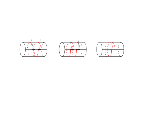
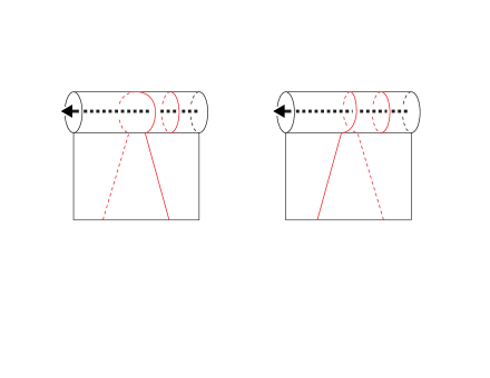
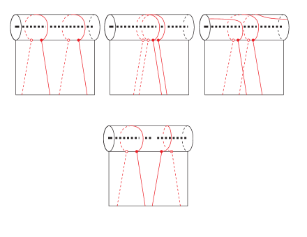
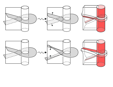
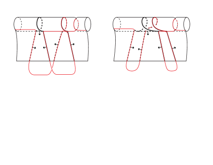
In summary, parametrize as so that represents the distinguished meridian , and represents the longitude , the isotopy class of . If we consider , for some tight , and focus on a neighourhood of one of or , then either as oriented arcs, or we see one of the models shown in Figure 2. Reversing the orientation convention found in [47, 48], we call the first transition arc positive and the second negative. Notice that reversing the orientation of reverses the orientation on , and vice versa; so, the sign of a transition arc is independent of the initial choice of orientation on . Either the endpoints of separate those of or they do not; up to symmetry, the possibilities when is not isotopic to (as unoriented arcs) are listed in Figure 3.
Remark 3.6.
We observe that the open book decomposition in associated to is right-veering (respectively, left-veering) [29] if, for every properly embedded tight oriented arc , either or the transition arc is positive (respectively, negative).
at 84 433 \pinlabel at 430 433 \pinlabel at 300 447 \pinlabel at 643 447 \pinlabel at 208 290 \pinlabel at 278 290 \pinlabel at 580 290 \pinlabel at 510 290 \pinlabel at 154 370 \pinlabel at 500 370 \pinlabelPositive transition [Bl] at 111 220 \pinlabelNegative transition [Bl] at 451 220 \endlabellist
at 141 480 \pinlabel at 450 480 \pinlabel at 697 480 \pinlabel at 385 190 \pinlabela at 385 340 \pinlabelb at 385 50 \endlabellist
Definition 3.7.
Given any metric space and any subset , the closed complement of in , denoted , is the metric completion of .
Remark 3.8.
Intuitively, amounts to cutting open along . (Although other authors have used the notation , we feel the inclusion of a vertical slash evokes the notion of “cutting.”) In particular, we will consider the closed complement of a curve in a surface and of a surface or, more generally, a lamination [25], in a -manifold, with respect to the path metric inherited from a Riemannian metric. For example, if is a fiber of a fibered knot , then is homeomorphic to .
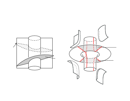
Definition 3.9.
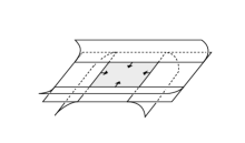
Let be a 3-manifold with nonempty boundary, and let be an oriented surface with nonempty boundary properly embedded in . Label the two copies of in by and . A product disk is an immersed disk in whose pre-image under the quotient map is properly embedded in with boundary consisting of two essential arcs in , and two essential arcs in , one contained in and one in . A product disk is tight if the two arcs of its boundary in are tight.
In particular, the disk of Notation 3.1 is a tight product disk whenever is tight.
3.2 Laminations and foliations
Roughly speaking, a codimension-one foliation of a 3-manifold is a disjoint union of surfaces injectively immersed in such that looks locally like . More precisely, we have the following definition.
Definition 3.10.
Let be a closed 3-manifold. A codimension one foliation of (or in) is a decomposition of into disjoint connected surfaces , called the leaves of , such that looks locally like . More precisely:
-
1.
, and
-
2.
there exists an atlas on with respect to which respects the following local product structure:
-
•
for every , there exists a coordinate chart in about such that is homeomorphic to and the restriction of to is the union of planes given by constant.
-
•
A foliation is co-oriented if the leaves admit co-orientations that are locally compatible.
We also consider foliations in compact smooth 3-manifolds with nonempty boundary, restricting attention to the case that is a nonempty union of tori and intersects everywhere transversely. In this case, at boundary points of , looks locally like horizontal closed half planes .
Calegari [4] proved that any foliation has an isotopy representative that is ; in particular, such that is defined and continuous, and leaves of are smoothly immersed. A foliation is taut [14, 6] if for every there exists a 1-submanifold that contains and is everywhere transverse to . The foliations constructed in this paper will have only noncompact leaves; hence they have an isotopy representative that is taut [27, 6].
Recall that a subset of is -saturated if it is a union of leaves of . A minimal set of is a closed -saturated subset of that doesn’t properly contain a nonempty closed -saturated subset. The foliations constructed in this paper contain a unique minimal set, and this minimal set is disjoint from .
A lamination is a decomposition of a closed subset of into a union of injectively immersed surfaces, called the leaves of , such that looks locally like , where is a closed subset of . Properly embedded compact surfaces, foliations, and -saturated closed subsets of , such as minimal sets of foliations, are all key examples of laminations. All laminations that arise in this paper are -saturated closed subsets of for some foliation .
A lamination strongly realizes the slope if it meets transversely in a lamination consisting of consistently oriented curves of slope . When is rational, these curves are closed, and it makes sense to talk about the manifold obtained by Dehn surgery along by slope . If a lamination strongly realizes slope , then it extends to a lamination in by capping off each boundary curve with disk. Moreover, if is a co-oriented taut foliation, then so is .
4 Any composite knot with a persistently foliar summand is persistently foliar.
Before discussing connected sums of fibered knots, we prove the useful fact that strong realization of a slope for a knot in extends to any connected sum with that knot.
Proposition 4.1.
Suppose is a connected sum of knots in . If the slope along is strongly realized by a co-oriented taut foliation, then so is the slope along .
Proof.
Suppose contains a co-oriented taut foliation that strongly realizes slope . By [20], there is a co-oriented taut foliation in that strongly realizes the longitudinal boundary slope. We describe how to form a “connected sum” of these two foliations to produce a co-oriented taut foliation that strongly realizes slope in .
Let denote a summing sphere for this connected sum, and set Observe that for each , is the union of two annuli, one of which is . Viewing as , we may arrange that each foliation intersects with leaves , . It is easy to check that, gluing to along , we obtain a taut foliation in that realizes slope . Choosing compatible co-orientations on the foliations and yields a co-orientation for . ∎
Corollary 4.2.
Suppose is a connected sum of knots. If at least one of the is persistently foliar, then so is .∎
5 Spines, Train Tracks and Branched surfaces
In this paper we construct foliations by first constructing a spine, which we then smooth to a branched surface that carries a foliation (more precisely, a lamination that extends to a foliation). We restrict attention to the case that any intersections of a spine or a branched surface with are transverse; hence the intersection of a branched surface with the boundary of a 3-manifold is a train track. The curves carried by this train track play an important role in our analysis.
A train track is a space locally modeled on one of the spaces of Figure 4. An -fibered neighbourhood of a train track is a regular neighborhood foliated (as a 2-manifold with corners) by interval fibers that intersect transversely, as locally modeled by the spaces in Figure 5.
1-manifold [B] at 195 135 \pinlabelneighborhood [B] at 195 95 \pinlabeldouble point [B] at 570 135 \pinlabelneighborhood [B] at 570 95 \endlabellist

1-manifold [B] at 170 100 \pinlabelneighborhood [B] at 170 70 \pinlabeldouble point [B] at 552 100 \pinlabelneighborhood [B] at 552 70 \endlabellist
A standard spine [5] is a space locally modeled on one of the spaces of Figure 6. A standard spine with boundary has the additional local models shown in Figure 7. The critical locus of is the 1-complex of points of where the spine is not locally a manifold. The critical locus is a stratified space (graph) consisting of triple points and arcs of double points .
Definition 5.1.
The components of are called the sectors of .
surface [B] at 170 200 \pinlabelneighborhood [B] at 170 170 \pinlabeldouble point [B] at 395 200 \pinlabelneighborhood [B] at 395 170 \pinlabeltriple point [B] at 615 200 \pinlabelneighborhood [B] at 615 170 \endlabellist
surface [B] at 235 215 \pinlabelneighborhood [B] at 235 185 \pinlabeldouble point [B] at 535 215 \pinlabelneighborhood [B] at 535 185 \pinlabelat boundary [B] at 235 155 \pinlabelat boundary [B] at 535 155 \pinlabel at 375 210 \endlabellist
A branched surface (with boundary) ([50]; see also [40, 41]) is a space locally modeled on the spaces of Figure 8 (along with those in Figure 9); that is, is homeomorphic to a spine, with the additional structure of a well-defined tangent plane at each point. The branching locus of is the 1-complex of points of where is not locally a manifold; such points are called branching points. The branching locus is a stratified space (graph) consisting of triple points and arcs of double points . The components of are called the sectors of .
surface [B] at 170 210 \pinlabelneighborhood [B] at 170 180 \pinlabeldouble point [B] at 390 210 \pinlabelneighborhood [B] at 390 180 \pinlabeltriple point [B] at 615 210 \pinlabelneighborhood [B] at 615 180 \endlabellist

surface [B] at 215 225 \pinlabelneighborhood [B] at 215 195 \pinlabeldouble point [B] at 535 225 \pinlabelneighborhood [B] at 535 195 \pinlabelat boundary [B] at 215 165 \pinlabelat boundary [B] at 535 165 \pinlabel at 355 220 \endlabellist
An -fibered neighborhood of a branched surface in a -manifold is a regular neighborhood foliated by interval fibers that intersect transversely, as locally modeled by the spaces in Figure 10 at interior points; if the ambient manifold has non-empty boundary, all spines and branched surfaces are assumed to be properly embedded, with a union (possibly empty) of I-fibers. The surface is a union of two subsurfaces, and , where , the vertical boundary, is a union of sub-arcs of I-fibers, and , the horizontal boundary, is everywhere transverse to the I-fibers.
Horizontal Boundary [Bl] at 270 345 \pinlabelVertical boundary [Br] at 270 310 \pinlabelsurface [B] at 120 105 \pinlabelneighborhood [B] at 120 75 \pinlabeldouble point [B] at 390 105 \pinlabelneighborhood [B] at 390 75 \pinlabeltriple point [B] at 635 105 \pinlabelneighborhood [B] at 635 75 \endlabellist
Let be the retraction of onto the quotient space obtained by collapsing each fiber to a point. The branched surface is obtained, modulo a small isotopy, as the image of under this retraction. We will freely identify with this image [40] and the core of each component of vertical boundary with its image in . Double points of the branching locus are cusps with cusp direction pointing inward from the vertical boundary if is viewed as the quotient of obtained by collapsing the vertical fibers to points. Cusp directions will be indicated by arrows, as in Figures 8 and 9.
A branched surface is co-oriented if the one-dimensional foliation of is oriented. When is a union of tori, and co-oriented is transverse to , the regions
are products, and we use the notation
Following Gabai [14, 19, 20], we call each component of a suture and refer to the pair as a sutured manifold. Note that each component of is an annulus or a torus.
A surface is said to be carried by if it is contained in and is everywhere transverse to the one-dimensional foliation of . A surface is said to be fully carried by if it carried by and has nonempty intersection with every I-fiber of . A lamination is carried by if each leaf of is carried by , and fully carried if, in addition, each I-fiber of has nonempty intersection with some leaf of .
Similarly, a 1-manifold, or union of 1-manifolds, is said to be carried by a train track if it is contained in some I-fibered neighbourhood , everywhere transverse to the one-dimensional foliation of . A 1-manifold, or union of 1-manifolds, is said to be fully carried by if it is carried by and has nonempty intersection with every I-fiber of .
at 243 360 \pinlabel at 295 327 \pinlabel at 285 270 \endlabellist
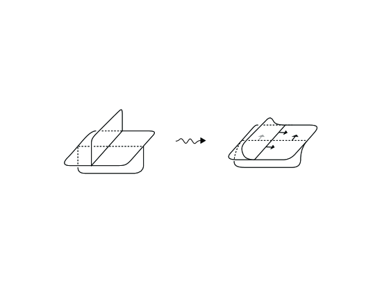
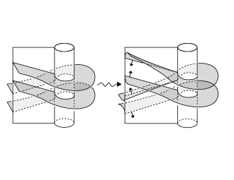
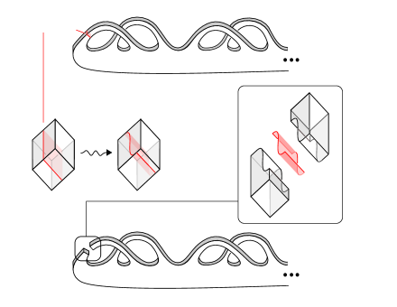
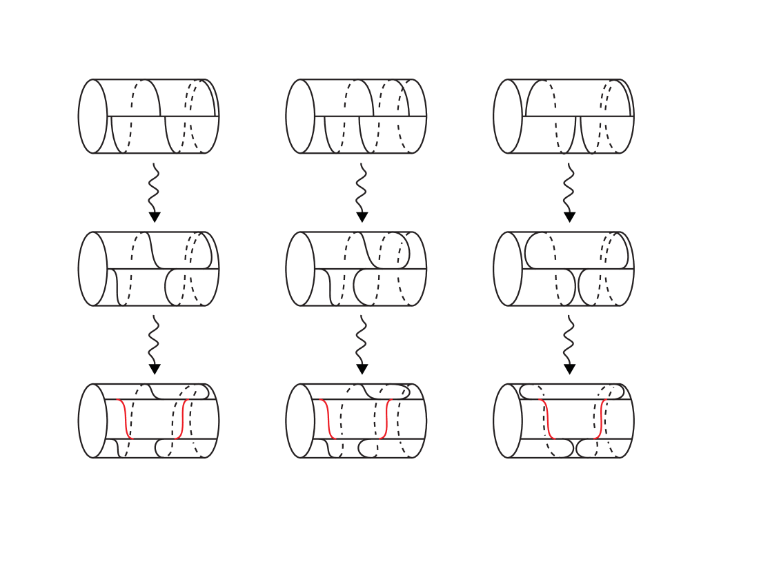
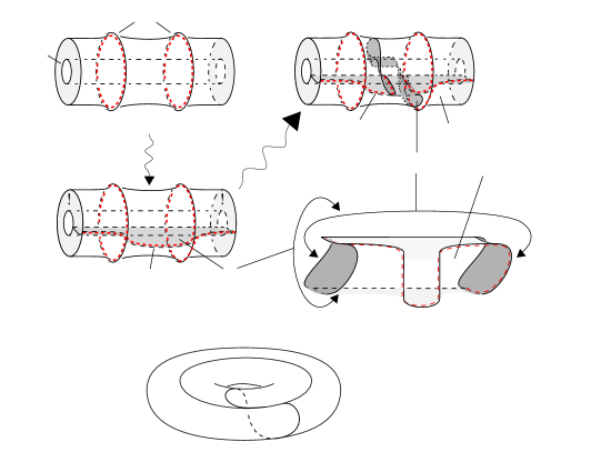
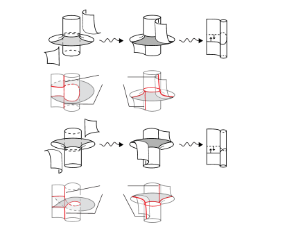
If a branched surface is homeomorphic to a spine , we say that is obtained by smoothing . An example is illustrated in Figure 11. We say that a choice of co-orientations on the sectors of is compatible if there is a smoothing of to a co-oriented branched surface that preserves the co-orientations on sectors; in this case, we call this smoothing the smoothing determined by the co-orientations. Examples are illustrated in Figure 12 and Figure 13. Branched surfaces as described below play a key role in this paper. We use the superscript because Lemma 5.3 describes a special case of Gabai’s Construction 4.16 of [20] applied in the context of [17].
Notation 5.2.
Let be a fibered 3-manifold, with compact fiber and monodromy ; assume is connected and non-empty. (For current purposes, of course, we focus on the complement of a fibered knot .) Let be a tight arc in such that (as unoriented arcs). Set . Any choice of orientations on the surfaces and determines a unique compatible smoothing of to a branched surface. We denote this branched surface by . (For purposes of this notation, and are assumed oriented.)
at 100 534 \pinlabel at 230 479 \pinlabel at 100 424 \pinlabel at 100 298 \pinlabel at 230 243 \pinlabel at 100 188 \pinlabel, showing [Bl] at 562 110 \pinlabelthe sutures, [Bl] at 562 85 \endlabellist
at 116 415 \pinlabel at 276 358 \pinlabel at 276 277 \endlabellist
Lemma 5.3.
The complement pair is homeomorphic to .
Proof.
The complement of is homeomorphic to , and hence is a handlebody of genus twice the genus of , with . Cutting along introduces two strips of vertical boundary with cores isotopic to , as illustrated in Figure 14, from which it follows that the complement of is homeomorphic to , with . ∎
at 102 558 \pinlabel at 375 490 \pinlabel at 375 62 \pinlabel at 622 185 \endlabellist
We next generalize the notation above for a particular family of splittings of the branched surface .
Notation 5.4.
Suppose is a sequence of pairwise tight oriented arcs properly embedded in , with .
Let , oriented so that contains as a positively oriented subarc. Let .
We denote by the branched surface obtained, under the identification , by smoothing the spine with co-orientation consistent with the given orientations on the product disks and copies of the fiber . Notice that is a splitting of for .
5.1 Laminar branched surfaces
A minimal set of a co-oriented taut foliation is necessarily essential, and therefore carried by an essential branched surface:
Definition 5.5.
[25] A branched surface in a closed 3-manifold is called an essential branched surface if it satisfies the following conditions:
-
1.
is incompressible in , no component of is a sphere and is irreducible.
-
2.
There is no monogon in ; i.e., no disk with , where is in an interval fiber of and
-
3.
There is no Reeb component; i.e., does not carry a torus that bounds a solid torus in .
In practice, it can be difficult to determine whether an essential branched surface fully carries a lamination. In [36, 37], Li defines the notion of laminar, a very useful criterion that is sufficient (although not necessary) to guarantee that an essential branched surface fully carries a lamination. We recall the necessary definitions here.
Definition 5.6.
Sink disks and half sink disks play a key role in Li’s notion of laminar branched surface. A sink disk or half sink disk can be eliminated by splitting open along a disk in its interior; these trivial splittings must be ruled out:
Definition 5.7.
Definition 5.8.
Theorem 5.9.
In general, the branched surface of Lemma 5.3 is not laminar. However, admits a splitting to a laminar branched surface. Moreover, this splitting can be chosen so that the boundary train track of the resulting laminar branched surface contains the meridian as subtrack.
Definition 5.10.
Let be an oriented fibered 3-manifold, with monodromy and compact fiber ; assume is connected and nonempty. Let be a tight arc properly embedded in . A sequence of oriented arcs properly embedded in is -sparse if, for all ,
-
1.
and
-
2.
and are non-isotopic.
Definition 5.11.
For , an -sparse sequence is -end-effective, if the endpoints give a monotonic sequence in the interval . An -sparse sequence is end-effective if it is both -end-effective and -end-effective.
Theorem 5.12.
Let be an oriented fibered 3-manifold, with monodromy and compact fiber ; assume is connected and nonempty. Let be a tight, non-separating, oriented arc properly embedded in such that (as oriented arcs). If both transition arcs are positive (respectively, negative), then there is a -end-effective (respectively, -end-effective) sequence such that the train track contains as subtrack the meridian, with the meridional subtrack necessarily containing (respectively, ).
If one transition arc is positive and the other negative, then there is an end-effective sequence such the train track contains as subtrack two disjoint copies of the meridian, with one component of the subtrack containing and the other containing .
In each case, the resulting branched surface is necessarily laminar.
Proof.
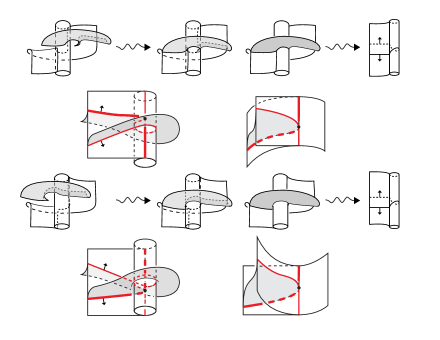
This is primarily a restatement of results found in [47, 48]. There are three possibilities, as illustrated in Figure 16.
When the transitions have a common sign and , this is the main result of [47] together with Corollary 6.4 of [48]. Corollary 6.4 of [48] is easily modified to allow for the case that ; a hint is shown in Figure 17. When the transitions are of opposite sign, this is the main construction of [47] together with Corollary 6.6 of [48]. ∎
[Bl] at 280 185 \pinlabel [Bl] at 613 185 \pinlabel [tr] at 192 148 \pinlabel [tr] at 524 148 \pinlabelor [Bl] at 406 143 \endlabellist
In particular, it follows that carries all meridians. (Recall that in this general context, a meridian is defined to be any curve having a single point of minimal transverse intersection with , and we use the definite article and the letter when referring to the distinguished meridian defined in Section 3.) When the transition arcs are of opposite sign, fully carries all meridians except . When both transition arcs have the same sign, fully carries all meridians except the two, which we call extremal, obtained by taking the union of with, respectively, each of the components of . When is positive (respectively, negative), the extremal meridians are and the simple closed curve of slope (respectively ). It follows that the train track fully carries the open interval of slopes that is bounded by these extremal meridians and contains all other meridians.
6 Connected sums of fibered knots are persistently foliar
Theorem 6.1.
Suppose and are nontrivial fibered knots in . Any nontrivial slope on is strongly realized by a co-oriented taut foliation that has a unique minimal set, disjoint from . Hence is persistently foliar.
Corollary 6.2.
Suppose is a connected sum of knots. If at least one of the is a nontorus alternating or Montesinos knot or a connected sum of fibered knots, then is persistently foliar.∎
Proof.
Corollary 6.3.
Suppose is a composite knot with a summand that is a nontorus alternating or Montesinos knot or the connected sum of two fibered knots, and is a manifold obtained by non-trivial Dehn surgery along . Then contains a co-oriented taut foliation; hence, satisfies the L-space Knot Conjecture.
We prove Theorem 6.1 in the sections that follow. First, in Section 6.1, we describe the spine, , underlying the branched surface, , that carries the minimal set of the desired foliations. In Section 6.2 we describe compatible co-orientations on , smoothing it to obtain . In Section 6.3 we give a precise description of the complementary regions of . In Section 6.4 we prove that carries no compact leaves, and in Section 6.5 we prove that fully carries a lamination. Finally, in Section 6.6, we show that this lamination extends to a family of co-oriented taut foliations with unique common minimal set, carried by , that strongly realize all boundary slopes.
6.1 The spine
Let be a connected sum, where each of the knots and is nontrivial and fibered, with fibers and respectively. Let denote the band connect sum of and ; so is a fiber for [13].
Let denote a summing sphere for this connected sum, cutting into and . Set
Choose the isotopy representatives of and so that for an arc properly embedded in . Thus and the endpoints of are fixed points of .
View as a compact surface properly embedded in , and view and as compact surfaces properly embedded in . Denote the component of containing by ; we observe that is indeed homeomorphic to the complement of . Let .
To simplify the exposition, we focus on the case that both and have right-veering monodromy. The case that they both have left-veering monodromy follows symmetrically. We address the remaining case, that has monodromy that is neither right- nor left-veering, in Section 7.
Choose non-separating, tight, properly embedded oriented arcs in and in disjoint from and such that , . Consider . Set Notice that is not yet a spine as two surfaces meet transversely along . To remedy this, isotope so that remains a properly embedded surface in , but is an isotopy representative of in that meets transversely in a single point. (We could instead have chosen this representative to be disjoint from . Now set
To simplify notation, set for .
Finally, isotope into the interior of , so that is parallel to , with the annulus still contained in the summing sphere .
6.2 The co-oriented branched surface
In this section, we describe a smoothing of by fixing a compatible choice of co-orientations on the sectors of .
at 245 464 \pinlabel at 485 464 \pinlabel at 355 455 \pinlabel at 258 440 \pinlabel at 400 470 \pinlabel at 500 440 \pinlabel at 185 345 \pinlabel at 580 345 \pinlabel at 258 250 \pinlabel at 360 235 \pinlabel at 500 250 \pinlabel at 285 230 \pinlabel at 525 230 \pinlabel at 415 212 \endlabellist
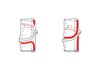
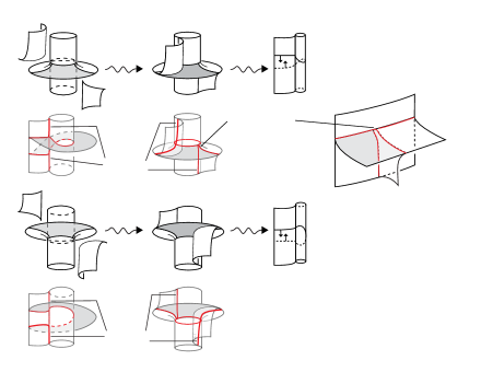
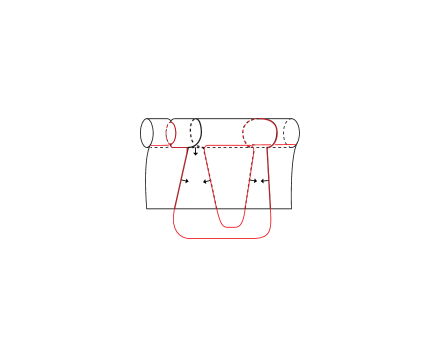
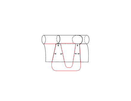
Choose a regular neighbourhood of in such that the closure of is disjoint from , and fix co-orientations on the sectors of as shown in Figure 18. Give and the co-orientations that agree, respectively, with the co-orientations of and . Choose any co-orientations on and . These induce orientations on and . Finally, cut open along (as defined in Notation 3.4) and assign co-orientations to the resulting annuli components to agree with those of . We have thus described co-orientations on the sectors of .
at 160 540 \pinlabel at 325 540 \pinlabel at 355 540 \pinlabelType C meridional smoothing [Bl] at 385 530 \pinlabel at 225 475 \pinlabel at 265 465 \pinlabel at 160 450 \pinlabel at 355 450 \pinlabel at 95 430 \pinlabel [Bl] at 378 425 \pinlabel at 450 430 \pinlabel at 123 388 \pinlabel at 160 330 \pinlabel at 265 340 \pinlabel at 355 330 \pinlabel at 297 325 \pinlabelType C [tr] at 130 305 \pinlabelmeridional smoothing [tr] at 130 270 \pinlabel at 160 255 \pinlabel at 193 252 \pinlabel at 363 252 \pinlabelBranching locus [Bl] at 270 80 \pinlabelon the annulus A [Bl] at 270 45 \endlabellist
It is straightforward to check that this choice of co-orientations on the sectors of determines a compatible smoothing of to a branched surface. Call this branched surface . The smoothings restricted to are shown in Figure 19. Those near and are shown in Figures 20 and 21, and called Type C, and those near and are shown in Figure 22, and called Type B. We note that the choice of co-orientations on the sectors of is motivated by the theory developed in [7, 8], as is the terminology Type C (for cusp) and Type B.
at 50 550
\pinlabel at 85 489
\pinlabel at 135 518
\pinlabelTriple point at at 535 430
\pinlabel at 305 550
\pinlabel at 292 506
\pinlabel at 212 485
\pinlabel at 225 526
\pinlabel at 247 492
\pinlabel at 180 515
\pinlabel at 557 535
\pinlabel at 490 505
\pinlabel at 579 484
\pinlabel at 653 515
\pinlabel at 641 486
\pinlabel at 509 465
\pinlabel at 190 402
\pinlabel at 145 357
\pinlabel at 120 280
\pinlabel at 75 260
\pinlabel [tr] at 90 328
\pinlabel [tr] at 88 296
\pinlabel [bl] at 182 345
\pinlabel [tl] at 172 328
\pinlabel at 410 380
\pinlabel at 375 365
\pinlabel at 350 300
\pinlabel at 380 280
\pinlabelBranch at 203 190
\pinlabelcurves at 203 165
\pinlabel at 340 170
\pinlabel at 300 152
\pinlabel at 265 81
\pinlabel at 303 70
\pinlabel at 655 215
\pinlabel at 545 184
\pinlabel at 627 183
\pinlabel at 690 165
\pinlabel at 550 135
\pinlabelTriple point at at 625 95
\endlabellist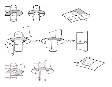
at 50 550 \pinlabel at 85 489 \pinlabel at 137 522 \pinlabelTriple point at at 540 430 \pinlabel at 180 520 \pinlabel at 210 550 \pinlabel at 290 530 \pinlabel at 300 488 \pinlabel at 227 511 \pinlabel at 247 545 \pinlabel at 557 470 \pinlabel at 480 500 \pinlabel at 580 516 \pinlabel at 641 520 \pinlabel at 655 490 \pinlabel at 502 539 \pinlabel at 80 390 \pinlabel at 120 370 \pinlabel at 143 291 \pinlabel at 190 250 \pinlabel [Br] at 93 330 \pinlabel [br] at 88 355 \pinlabel [tl] at 182 302 \pinlabel [Bl] at 172 330 \pinlabel at 380 370 \pinlabel at 350 355 \pinlabel at 375 285 \pinlabel at 410 270 \pinlabel at 303 160 \pinlabel at 265 150 \pinlabel at 300 81 \pinlabel at 340 70 \pinlabelBranch at 201 65 \pinlabelcurves at 201 40 \pinlabel at 650 90 \pinlabel at 533 157 \pinlabel at 615 120 \pinlabel at 688 140 \pinlabel at 517 132 \pinlabelTriple point at at 630 65 \endlabellist
at 92 539 \pinlabel at 145 518 \pinlabel at 70 490 \pinlabel at 114 567 \pinlabel at 135 550 \pinlabel at 162 528 \pinlabel at 114 495 \pinlabel at 85 493 \pinlabel at 398 553 \pinlabel at 310 527 \pinlabel at 373 518 \pinlabel at 305 490 \pinlabel at 349 567 \pinlabel at 326 530 \pinlabel at 375 555 \pinlabel at 349 495 \pinlabel at 323 495 \pinlabel at 430 518 \pinlabel at 510 560 \pinlabel at 486 530 \pinlabel at 545 555 \pinlabel at 510 505 \pinlabel at 475 500 \pinlabel at 478 450 \pinlabel at 485 390 \pinlabel at 470 315 \pinlabel [l] at 258 396 \pinlabel [Bl] at 537 380 \pinlabelTriple point [Bl] at 590 408 \pinlabelat [Bl] at 590 378 \pinlabel at 164 277 \pinlabel at 53 265 \pinlabel at 135 240 \pinlabel at 65 215 \pinlabel at 70 270 \pinlabel at 112 250 \pinlabel at 150 245 \pinlabel at 80 218 \pinlabel at 400 275 \pinlabel at 310 250 \pinlabel at 372 237 \pinlabel at 302 215 \pinlabel at 350 278 \pinlabel at 325 255 \pinlabel at 387 275 \pinlabel at 350 220 \pinlabel at 317 218 \pinlabel at 431 245 \pinlabel at 505 282 \pinlabel at 477 250 \pinlabel at 553 275 \pinlabel at 505 220 \pinlabel at 472 218 \pinlabel at 485 173 \pinlabel at 485 90 \pinlabel at 460 32 \pinlabel [l] at 258 88 \pinlabel [Bl] at 537 90 \pinlabelTriple point [Bl] at 590 115 \pinlabelat [Bl] at 590 85 \endlabellist
It is helpful for calculations to make note of the components of that result locally from each type of smoothing near a transition arc. These are shown in (red) boldface in Figure 23.
Type A or C [B] at 220 165 \pinlabelType B [B] at 560 165 \endlabellist
6.3 The three complementary regions of
For each , let denote the genus of . We now describe the components of the sutured manifold , commonly referred to as the complementary regions of . Clearly there are three, one of which contains , and one lying in each . Let and be the annuli of vertical boundary with cores and .
Proposition 6.4.
The sutured manifold consists of the following three (sutured manifold) components:
-
1.
,
-
2.
, and
-
3.
,
where is a surface with two boundary components and genus .
Proof.
is parallel to . Moreover, each of the two Type C neighbourhoods of introduces a single meridian suture. Hence, the complementary region containing is isomorphic to the sutured manifold described in (1).
Set and . By Lemma 5.3, it suffices to show that the remaining components complementary to are isomorphic as sutured manifolds to the closed complements of and , respectively. Let be the component that lies in . Forgetting the sutured manifold structure of , the compact 3-manifold is a genus handlebody, and hence is homeomorphic to . It suffices, therefore, to prove that this homeomorphism can be chosen so that is mapped to . Away from and the crossings , the core of runs along , parallel to . At the crossings, this core combines with the arcs (topologically) as it does in ; see Figure 23.
At , this core wraps partway about , but disjointly from . Hence is isomorphic to This is illustrated in Figure 24. ∎
Type C at 145 570 \pinlabelType B at 245 570 \pinlabelType C at 515 570 \pinlabelType B at 600 570 \pinlabel [Br] at 120 405 \pinlabel [Br] at 183 405 \pinlabel [Bl] at 201 405 \pinlabel [Bl] at 268 405 \pinlabel [Br] at 483 405 \pinlabel [Bl] at 520 405 \pinlabel [Br] at 610 405 \pinlabel [Bl] at 645 405 \endlabellist
Corollary 6.5.
Let denote a closed 3-manifold obtained by Dehn filling of slope along . The complement consists of the following three components:
-
1.
A solid torus whose meridian has minimal geometric intersection number with ,
-
2.
, and
-
3.
,
where is a surface with two boundary components and genus .
Proof.
Consider the complementary component that contains . After Dehn filling with slope , this component transforms to a solid torus with meridian intersecting each of the curves and minimally in points. ∎
6.4 Any leaf carried by is noncompact.
Proposition 6.6.
Any surface carried by has nonempty intersection with every branch of , and is noncompact. In particular, does not carry a torus.
Proof.
Let be any nonempty surface carried by , and let be the sub-branched surface of that fully carries . If fully carries , then . In general, is a union of sectors of .
We first observe that must contain a sector of that has nonempty intersection with . Suppose by way of contradiction that it does not. Since the sink directions on point into for each , contains such a sector of whenever contains ; hence we may assume that contains no . But if does not contain or , it can contain a sector of only when it contains every sector of . Hence, we may assume that does not contain , , or any sector of , and therefore does not contain any sector of , since a cusp direction points from into at Type C smoothings. But it then follows that cannot contain a sector of , and hence is empty, an impossibility.
Thus, contains a sector of that has nonempty intersection with . Since has an arc of boundary along with outward-pointing cusp direction, contains a proper embedding of a ray carried by a meridian of ; hence, is not compact. ∎
6.5 fully carries a lamination
The branched surface might contain sink or half sink disks. However, using ideas from [48], it is straightforward to show that it can be split to a branched surface that contains no sink or half sink disk.
Notation 6.7.
Given a sequence of oriented arcs embedded in , let , oriented so that contains as a positively oriented subarc. Let .
Proposition 6.8.
The branched surface can be split open to a laminar branched surface homeomorphic to the spine
where is a -end-effective sequence in .
The complement of has components:
-
1.
, where and are disjoint meridional annuli,
-
2.
copies of , and
-
3.
copies of ,
where each is a surface with two boundary components and genus .
Proof.
Recall our assumption that all transition arcs are positive; hence Type B smoothings occur at and Type C smoothings occur at for each arc , .
at 125 365 \pinlabel at 300 365 \pinlabel [tr] at 105 330 \pinlabel [tl] at 335 270 \pinlabel at 135 290 \pinlabel at 280 290 \pinlabel at 620 418 \pinlabel at 465 380 \pinlabel at 550 374 \pinlabel at 550 280 \pinlabel at 458 190 \pinlabel at 612 152 \pinlabel [l] at 685 243 \pinlabel [l] at 702 323 \endlabellist
Applying Theorem 5.12 to , for each , there are -end-effective sequences such that each branched surface is laminar, and each train track , contains the meridian as a subtrack containing . Denote each meridian subtrack by . Recall that each is oriented consistently with , .
Setting
we describe a smoothing of by fixing a compatible choice of co-orientations on the sectors of . Indeed, co-orientations have been fixed for all sectors except those lying in . We define co-orientations in the sectors of by choosing co-orientations on the two annuli obtained by cutting open along , choosing these co-orientations to agree with the co-orientations chosen on .
It is straightforward to check that this choice of co-orientations on the sectors of determines a compatible smoothing of to a branched surface. Call this branched surface . Under this smoothing, the two meridians become meridian cusps in the complementary region that contains . This is illustrated in Figure 25. Let be the annulus of vertical boundary with core .
Since does not carry a torus, and is a splitting of , does not carry a torus. Moreover, since the sequences are -sparse, neither has a sink disk or half sink disk; thus, has no sink disk or half sink disk. So is laminar. ∎
Corollary 6.9.
fully carries a lamination.
6.6 extends to co-oriented taut foliations that strongly realize all boundary slopes
Proposition 6.10.
For each slope (not necessarily rational), the lamination extends to a co-oriented taut foliation that strongly realizes . Each has a unique minimal set, fully carried by .
Proof.
The complementary region of that is not a product (as a sutured manifold) is the one containing : , where and are disjoint meridional annuli. Denote this region by . We will now show that for every nontrivial slope (not necessarily rational), this region can be filled in by noncompact leaves that meet in parallel leaves of slope .
When is rational, this region contains a properly embedded annulus . When is not the meridian, any choice of co-orientation of describes a smoothing of to a branched surface in whose complementary regions are all products (as sutured manifolds).
In general (when is either rational, but not the longitude , or irrational), proceed instead as follows. Consider the essential annulus . Again, any choice of co-orientation of describes a smoothing of to a branched surface in whose complementary regions are all products. In particular, the complementary region is a solid torus with two longitudinal sutures (one of which is ). Let be the product disk for this region, isotoped so that the essential arcs are disjoint. The two distinct choices of orientation on give rise to two smoothings of ; call the resulting branched surfaces and . The isotopy representative of can be chosen so that the train tracks and together fully carry all nontrivial, nonlongitudinal boundary slopes. The associated measures on these train tracks describe measured laminations that are fully carried by the sub-branched surfaces (not properly embedded) with spine . See Figure 26. (Alternatively, the branched surfaces and are laminar, and hence there exist co-oriented laminations fully carried by or that strongly realize any nontrivial, nonlongitudinal slope [37]. The proof of the main result of [37] reveals that these foliations can be chosen to include as a sublamination.) This argument can of course be repeated replacing with any nontrivial rational slope.
Branch curves at 190 595 \pinlabel [Bl] at 25 545 \pinlabel! at 88 548 \pinlabel! at 285 548 \pinlabel (Identify annuli marked “!”) at 190 450 \pinlabel! at 398 548 \pinlabel! at 596 548 \pinlabelBranch curve at 460 448 \pinlabelHalf-disk [Bl] at 572 432 \pinlabelproduct sutured [Bl] at 572 410 \pinlabelmanifold component [Bl] at 572 388 \pinlabel at 545 398 \pinlabelBranch curve at 190 255 \pinlabel at 302 260 \pinlabel(Cut open on and ) at 535 190 \pinlabel at 170 95 \pinlabel at 230 100 \pinlabel at 283 100 \pinlabel at 350 75 \pinlabel at 413 125 \pinlabel at 396 75 \pinlabelSlope = (in terms of ) at 320 22 \endlabellist
Filling in the product complementary regions of the resulting lamination with parallel copies of the boundary leaves yields a co-oriented foliation that strongly realizes . Since has no compact leaves, it is necessarily taut. Since any leaf carried by has nonempty intersection with every branch of , has exactly one minimal set. When the surgery coefficient is rational but not an integer, the minimal set of remains genuine after Dehn filling by slope . ∎
This extension of to the family of co-oriented taut foliations (and ) is an extension of the well known “stacking chair” construction (see, for example, Example 1.1.i in [22]). An alternate approach to moving from the lamination to co-oriented taut foliations in , for rational, can be found as Operations 2.3.2 and 2.4.4 in [21].
We note, for the reader interested in understanding all co-oriented taut foliations in the complement of , that there are multiple distinct choices of compatible co-orientations on leading to branched surfaces that fully carry taut foliations.
7 Additional constructions when the monodromy of is neither right- nor left-veering.
Recall that if the monodromy of is neither right- nor left-veering, Theorem 1.4 guarantees that any nontrivial slope is strongly realized by some co-oriented taut foliation. We now introduce several new constructions of co-oriented taut foliations that give the same result, most of which differ from the foliations of [47, 48] in that they have genuine minimal set.
We note in passing that if the monodromy of is neither right- nor left-veering, then it has fractional Dehn twist coefficient zero [30], or, equivalently, Gabai degeneracy for some [34].
Lemma 7.1.
A connected sum of fibered knots in has right-veering (respectively, left-veering) monodromy if and only if each of its components has right-veering (respectively, left-veering) monodromy.
Proof.
By induction, it suffices to consider the case of two nontrivial summands. The result follows immediately from Corollary 1.4 of [16], or, more directly, from an analysis of product disks. ∎
Corollary 7.2.
Suppose is a fibered knot in . If the monodromy is neither right- nor left-veering, then one of the following must be true:
-
1.
at least one of or has monodromy that is neither right- nor left-veering, or
-
2.
one of or has monodromy that is right-veering, and the other summand is left-veering. ∎
We proceed as in the right-veering case, by first constructing a spine, and then describing a smoothing by fixing a compatible choice of co-orientations on the branches of this spine. We note for completeness that we could address each summand separately in the manner of Section 6: as in Section 6.1, let , with the orientations on , and chosen as before in Section 6.2. The only difference in the case that has transition arcs of opposite sign is that, along with a local smoothing of Type C, we see a local smoothing as shown in Figures 27 and 28, which we call Type A; again, as before, the sutures of agree with those of , as shown in Figure 29.
at 60 540 \pinlabel at 105 530 \pinlabel at 105 492 \pinlabel at 105 463 \pinlabel at 149 453 \pinlabel at 285 516 \pinlabel at 315 530 \pinlabel at 315 493 \pinlabel at 314 469 \pinlabel at 342 474 \pinlabel at 280 387 \pinlabel at 315 400 \pinlabel at 315 359 \pinlabel at 315 340 \pinlabel at 342 341 \pinlabelTriple point at 428 415 \pinlabelBranch [Bl] at 165 332 \pinlabelcurves [Bl] at 165 310 \pinlabel at 625 420 \pinlabel at 695 382 \pinlabel at 600 365 \pinlabel at 672 347 \pinlabel at 640 335 \pinlabel at 570 325 \pinlabel at 53 278 \pinlabel at 100 193 \pinlabel at 100 265 \pinlabel at 100 235 \pinlabel at 142 185 \pinlabel at 277 252 \pinlabel at 307 197 \pinlabel at 310 260 \pinlabel at 310 235 \pinlabel at 335 205 \pinlabel at 277 119 \pinlabel at 307 64 \pinlabel at 310 129 \pinlabel at 310 102 \pinlabel at 338 70 \pinlabelBranch [Bl] at 168 50 \pinlabelcurves [Bl] at 168 28 \endlabellist
at 230 555 \pinlabel at 185 545 \pinlabel at 185 505 \pinlabel at 185 475 \pinlabel at 137 463 \pinlabel at 422 535 \pinlabel at 392 545 \pinlabel at 395 505 \pinlabel at 395 480 \pinlabel at 360 485 \pinlabel at 425 389 \pinlabel at 392 400 \pinlabel at 395 360 \pinlabel at 395 335 \pinlabel at 360 343 \pinlabelBranch [Bl] at 256 421 \pinlabelcurves [Bl] at 256 399 \pinlabel at 235 285 \pinlabel at 190 272 \pinlabel at 190 243 \pinlabel at 190 205 \pinlabel at 147 198 \pinlabel at 425 260 \pinlabel at 392 265 \pinlabel at 395 240 \pinlabel at 398 210 \pinlabel at 370 220 \pinlabel at 425 120 \pinlabel at 392 122 \pinlabel at 395 100 \pinlabel at 400 65 \pinlabel at 367 73 \pinlabelBranch [Bl] at 256 135 \pinlabelcurves [Bl] at 256 114 \endlabellist
Type C [B] at 355 410 \pinlabelType A [B] at 462 410 \pinlabel [Br] at 325 260 \pinlabel [Br] at 387 260 \pinlabel [Br] at 452 260 \pinlabel [Br] at 489 260 \endlabellist
However, there is a simpler and more general construction which does not depend on having a connected sum, given in the following proposition:
Theorem 7.3.
Suppose that is a fibered 3-manifold, with fiber a compact oriented surface with connected boundary, and orientation-preserving monodromy . If there is a tight arc so that the corresponding product disk has transition arcs of opposite sign, then there is a co-oriented taut foliation that strongly realizes slope for all slopes except , the distinguished meridian. The foliation has a unique minimal set, and this minimal set is genuine and disjoint from . Furthermore, each extends to a co-oriented taut foliation in , the closed 3-manifold obtained by Dehn filling along , and when intersects the meridian efficiently in at least two points, the minimal set of is genuine as well.
Type C [B] at 355 410 \pinlabelType C [B] at 462 410 \pinlabel [Br] at 325 260 \pinlabel [Br] at 387 260 \pinlabel [Br] at 452 260 \pinlabel [Br] at 489 260 \endlabellist
Proof.
Set , , and . Choose a small annular neighbourhood of in , and let denote the complement of this annulus in . We may assume restricts to a homeomorphism of ; so is a codimension zero submanifold of . Let denote the torus boundary of this submanifold.
Now consider the spine . Fix an arbitrary co-orientation on , and choose the co-orientation on that results in the smoothing in the interior of that is indicated in Figure 30.
Now choose co-orientations on the components of in a neighbourhood of the spine about each transition so that a meridian cusp in introduced at each, as modelled in Figures 20 and 21. Since the transition arcs are of opposite sign, there is a compatible choice of co-orientation on the components of that agrees with these local choices. As illustrated in Figure 30, the complementary region of the resulting branched surface that does not contain is isomorphic as a sutured manifold to . We thus obtain a branched surface with one complementary region homeomorphic to a , where , and one complementary region homomorphic to , where and are disjoint meridional annuli with cores and , respectively. It is therefore essential. Apply the arguments of Section 6 to the splitting of guaranteed by Theorem 5.12 to see that splits to a laminar branched surface. The desired conclusions now follow as in our previous constructions. ∎
References
- [1] S. Boyer and A. Clay, Foliations, orders, representations, L-spaces and graph manifolds, Adv. Math. 310 (2017), 159–234.
- [2] S. Boyer, C. Gordon and L. Watson, On L-spaces and left-orderable fundamental groups, Math. Ann. 356 (2013), no. 4, 1213–1245.
- [3] G. Burde and H. Zieschang, Knots, De Gruyter Studies in Mathematics, 5. Walter de Gruyter and Co., Berlin, 2003.
- [4] D. Calegari, Leafwise smoothing laminations, Algebr. Geom. Topol. 1 (2001), 579–585.
- [5] B. Casler, An imbedding theorem for connected 3-manifolds with boundary, Proc. A.M.S. 16 (1965), 559–566.
- [6] V. Colin, W. H. Kazez and R. Roberts, Taut foliations, 2016, ArXiv:1605.02007 (to appear in Comm. Anal. Geom.).
- [7] C. Delman and R. Roberts, Nontorus alternating knots are persistently foliar, preprint.
- [8] C. Delman and R. Roberts, Persistently foliar Montesinos knots, preprint.
- [9] C. Delman and R. Roberts, Montesinos knots satisfy the L-space knot conjecture, preprint.
- [10] C. Delman and R. Roberts, Taut double-diamond replacements, preprint.
- [11] C. Delman and R. Roberts, Modifying branched surfaces at the boundary, in preparation.
- [12] J. Etnyre and J. Van Horn-Morris, Fibered Transverse Knots and the Bennequin Bound, IMRN 2011 (2011), 1483–1509.
- [13] D. Gabai The Murasugi sum is a natural geometric operation, Contemp. Math. 20 (1983), 131-143.
- [14] D. Gabai, Foliations and the topology of 3-manifolds, J. Differential Geom. 18 (1983), no. 3, 445–503.
- [15] D. Gabai, Foliations and genera of links, Topology 23 (1984), 381–394.
- [16] D. Gabai, The Murasugi sum is a natural geometric operation II, Contemp. Math. 44 (1985), 93–100.
- [17] D. Gabai, Detecting fibered links in , Comment. Math. Helvetici 61 (1986), 519–555.
- [18] D. Gabai, Genera of the arborescent links, Memoirs of the AMS 59 (339) (1986), 1–98.
- [19] D. Gabai, Foliations and the topology of 3-manifolds. II, J. Differential Geom. 26 (1987), no. 3, 461–478.
- [20] D. Gabai, Foliations and the topology of 3-manifolds. III, J. Differential Geom. 26 (1987), no. 3, 479–536.
- [21] D. Gabai, Taut foliations and suspensions of , (1992),
- [22] D. Gabai, Problems in foliations and laminations, Geometric Topology (ed. W. Kazez), Proceedings of the 1993 Georgia International Topology Conference; 2 (1997), 1–33.
- [23] D. Gabai, Essential laminations and Kneser normal form, J. Diff. Geom. 53 (1999), 517–574.
- [24] D. Gabai and W. Kazez, Homotopy, Isotopy and Genuine Laminations of 3-Manifolds, Geometric Topology, Vol 1, (W H Kazez Ed.) AMS/IP (1997) 123–138.
- [25] D. Gabai and U. Oertel, Essential Laminations in 3-Manifolds, Ann. Math. 130, (1989), 41–73.
- [26] P. Ghiggini, Knot Floer homology detects genus-one fibred knots, Amer. J. Math. 130 (2008), no. 5, 1151–1169.
- [27] A. Haefliger, Variétés feuilletées, Ann. Scuola Norm. Sup. Pisa (3) 16 (1962), 367–397.
- [28] M. Hirasawa and K. Murasugi, Genera and fibredness of Montesinos knots, Pac. J. Math 225(1) (2006), 53–83.
- [29] K. Honda, W. Kazez and G. Matić, Right-veering diffeomorphisms of compact surfaces with boundary, Invent. Math. 169, (2007), 427–449.
- [30] K. Honda, W. Kazez, G. Matić, The contact invariant in sutured Floer homology, Invent. Math. 176 (2009), no. 3, 637–676.
- [31] A. Juh/’asz, Floer homology and surface decompositions, Geom. Topol. 12 (2008), 299–350.
- [32] A. Juh/’asz, The sutured Floer homology polytope, Geom. Topol. 14 (2010), 1303–1354.
- [33] A. Juh/’asz, A survey of Heegaard Floer homology, New Ideas in Low Dimensional Topology, World Scientific (2014), 23–296.
- [34] W. H. Kazez and R. Roberts, Fractional Dehn twists in knot theory and contact topology, Algebr. Geom. Topol. 13(6), (2013), 3603–3637.
- [35] D. Krcatovich, The reduced knot Floer complex, Topol. Appl. 194 (2015) 171-201.
- [36] T. Li, Laminar branched surfaces in 3-manifolds, Geom. Top. 6 (2002), 153–194.
- [37] T. Li, Boundary train tracks of laminar branched surfaces, Topology and geometry of manifolds (Athens, GA, 2001), 269–-285, Proc. Sympos. Pure Math., 71, Amer. Math. Soc., Providence, RI, 2003.
- [38] Y. Ni, Knot Floer homology detects fibred knots, Invent. Math. 170 (2007), 577–608.
- [39] Y. Ni, Erratum: Knot Floer homology detects fibred knots, Invent. Math. 170 (2009), no. 1, 235–238.
- [40] U. Oertel, Incompressible branched surfaces, Invent. Math. 76 (1984), 385–410.
- [41] U. Oertel, Measured laminations in 3-manifolds, Trans, A.M.S. 305 (1988), 531–573.
- [42] P. Ozsváth and Z. Szabó, Holomorphic disks and genus bounds, Geom. Topol. 8 (2004), 311–334.
- [43] P. Ozsváth and Z. Szabó, Holomorphic disks and topological invariants for closed 3-manifolds, Ann. Math. 159(3), (2004), 1027–1158.
- [44] P. Ozsváth and Z. Szabó, Holomorphic disks and three-manifold invariants: properties and applications, Ann. of Math. (2), 159 (3) (2004), 1159–1245.
- [45] P. Ozsváth and Z. Szabó, On Heegaard diagrams and holomorphic disks, European Congress of Mathematics, Eur. Math. Soc., Z/”urich, 2005, 769–781.
- [46] P. Ozsváth and Z. Szabó, Heegaard Floer homology and contact structures, Duke Math. J. 129(1)(2005), 39–61.
- [47] R. Roberts, Taut foliations in punctured surface bundles. I, Proc. London Math. Soc. (3) 82 (2001), no. 3, 747–768.
- [48] R. Roberts, Taut foliations in punctured surface bundles, II. Proc. London Math. Soc. (3) 83 (2001), no. 2, 443–471.
- [49] J. Stallings, Constructions of fibered knots and links, Proc. Symp. Pure Math. AMS 27 (1975), 315-319.
- [50] R. Williams, Expanding attractors, Inst. Hautes Études Sci. Publ. Math. 43 (1974), 169–203.