Multi-Agent Image Classification via Reinforcement Learning

Abstract

We investigate a classification problem using multiple mobile agents capable of collecting (partial) pose-dependent observations of an unknown environment. The objective is to classify an image over a finite time horizon. We propose a network architecture on how agents should form a local belief, take local actions, and extract relevant features from their raw partial observations. Agents are allowed to exchange information with their neighboring agents to update their own beliefs. It is shown how reinforcement learning techniques can be utilized to achieve decentralized implementation of the classification problem by running a decentralized consensus protocol. Our experimental results on the MNIST handwritten digit dataset demonstrates the effectiveness of our proposed framework.

I Introduction

With the rising interest in the Internet of Things (IoT), the demand for design of autonomous agents that are capable of cooperation is increasing. The interconnected robots will be major players in the future, accomplishing many duties in industrial automation[1], military support[2], and health-care[3]. In many of these applications, a major issue is that every agent has limited sensing capabilities, and therefore, may not have sufficient information for accomplishing a complex task. One way to mitigate this shortcoming is to let the task to be solved collectively by multiple agents. In the context of machine learning, this means that the agents need not only to learn through individual interaction with their environment but also they can learn from each others’ experiences using communication.

In several machine learning applications, the problem suffers from the high-dimension of the feature space, which may render the learning process inefficient. One may list facial element recognition, genome disorder identification, or fault detection as instances of problems facing these issues. In these examples, the main challenge is that a large portion of the input data might be irrelevant to the task. One possibility is to pre-process the data to filter the irrelevant pieces of information. However, this might be challenging or cause data inaccuracy. In this paper, we propose an approach that may provide an alternative mechanism for complexity reduction: we translate the classification task into a multi-agent reinforcement learning setting, where the space of observations per agent has a comparatively lower dimension.

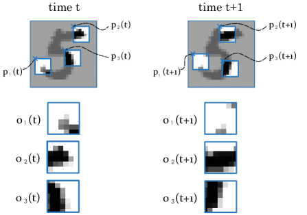
Figure 1: This example illustrates why classification through local observations of an agent is challenging. The observations made by $3$ agents at two consecutive time instants have been magnified, where the spatial variables dictate the observations. This highlights the need for a communication and memory mechanisms.

In this work, we study the multi-agent image classification problem within an unknown environment. The setup consists of an environment, in which multiple homogeneous agent,s each with a partial observation of the environment, are collaborating to do a classification task. To explore the environment efficiently, the agents need to learn how to optimally traverse the environment and receive new observations through re-positioning. Moreover, they are capable of establishing autonomous communication to update their beliefs. This is motivated by the idea that a more experienced teammate could provide or explain hints, which can be used to facilitate the perception. We are interested in maximizing a long-term collective reward that pushes the agents to effectively coordinate and cooperate in order to correctly classify the image. Our goal in this work is to approach this classification task through an end-to-end co-design of decentralized data-processing, communication, action planning, and prediction modules on each agent (see Fig. 1 for an example).

For solving this problem, we formulate it within a multi-agent reinforcement learning framework and propose a policy gradient, which can effectively optimize the agents’ behavior. In contrast to the vanilla policy gradient settings, our framework introduces a differentiable reward rather instead of a reward that is independent of the network parameters. The proposed mechanism enables the policy gradient algorithm to not only maximize the probability of generating desirable outcomes, but also to explicitly increase the rewards. The mathematical derivation of the latter argument is given in Section IV, which generalizes the policy gradient approach for the case of differentiable rewards.

We have demonstrated a descent performance of the proposed framework in the MNIST classification task. We can correctly classify 88% of the testing dataset by using two agents, each only with 2$\times$2 pixels observations. We observe that with larger observations or longer communications, the prediction quality further increases up to 97.75%.

II Problem Statement

Suppose that $N$ identical agents are in a static unknown environment. Let the agents start from a pre-determined spatial configuration. At each time step, each agent is capable of collecting a partial observation from the environment, performing some local data processing, and communicating the result with neighboring agents. The agents are allowed to communicate over a directed graph, where neighbors of an agent are those whose messages can be received by that agent. We assume that each agent knows its own pose with respect to the environment and can take certain actions to move and update its pose at each time step. The collective objective of these agents is to classify the instance of the environment from a finite number of possibilities $\{1,2,\dots,M\}$ over a finite time horizon.

In order to decentralize the process throughout the execution, the actions by each agent should be decided solely based on the local information available to them. As a result, agents need to learn how to communicate, extract relevant features and specifications from partial observations, navigate in the environment, and reliably solve the classification problem.

In Section IV, we propose a modular architecture for the network of multiple agents and discuss the details of different modules of an agent to achieve decentralized classification. In Section VI, we demonstrate the required steps for learning the design parameters using reinforcement learning.

III Connections to the Literature

In most of the multi-agent reinforcement learning literature, it is typical to assume that the agents are non-identical since their respective policies might be very distinct[4, 5]. Even though this assumption might be non-avoidable in some applications, assuming the existence of a common shared policy for all agents can be helpful, especially when their policies can be distinguished via some visible characteristics e.g., their location. Among the literature, [6] has considered a similar setup for the homogeneity of the agents. This assumption provides an advantage: the agents can learn from each others’ experience. A similar idea is followed in [7], where an agent interacts with multiple instances of an environment, allowing her to learn from a concurrent stream of experiences. Even though they study a single-agent scenario, the homogeneity assumption allows approaching this multi-agent problem as a single-learner problem.

In series of works on multi-agent reinforcement learning, the focus is on cases where the data is spread over a number of agents and the goal is to conduct the training in a distributed or decentralized manner. For instance, a promising framework for this purpose is the Federated Learning, where the goal is to conduct the stochastic gradient descent by combining partially computed gradients over different agents [8, 9, 10]. Contrary to this line of research, we consider settings in which the agents need to communicate throughout the execution as well.

In a more related paper, the authors of [5] consider a value function approximation approach for decentralized learning with interconnected agents and bring operational guarantees in the case of linear value functions. A similar multi-agent learning problem is addressed in [11], where deep neural networks are used as function approximators. A generalization of this problem within an actor-critic scenario appears in [12]. Contrary to these works, we address the case where each data point is observed by a number of agents that are collaborating to fulfill a task (e.g., see Fig. 1), while the next set of observations are affected by (locally) decided actions of the agents. Moreover, in our settings, the reward for reinforcement learning becomes differentiable. This necessitates revisiting the derivation of the policy gradients.

Another related line of research concerns the end-to-end design of distributed or decentralized control architectures, where the goal is to learn optimal control laws in a setting with multiple dynamic agents [13, 14, 15].

III-A Notations and Preliminaries

The set of real numbers, nonnegative real numbers, and nonnegative integer numbers are denoted by $\mathbb{R}$, $\mathbb{R}_{+}$ and $\mathbb{Z}_{+}$, respectively. Other sets are denoted by script letters; e.g., $\mathcal{A}$ while their cardinality is denoted by $|\mathcal{A}|$. We use bold letters to denote maps; e.g., $\mathbf{g}(x)$. The trainable parameter of a map is denoted by $\theta_{i}$ appearing as a subscript; e.g., $\mathbf{f}_{\theta_{1}}$. The map $\mathbf{{SoftMax}}(x):\leavevmode\nobreak\ \mathbb{R}^{M}\rightarrow\mathbb{R}_{+}^{M}$ is standard softmax with $k$’th element given by ${\exp(x_{k})}/{\sum_{i=1}^{M}\exp(x_{i})}.$ A directed graph $\mathcal{G}$ is characterized by a set of nodes (or vertices) $\mathcal{V}:=\{1,2,\dots,N\}$ and a set of directed edges (or arcs) denoted as $\mathcal{E}\subset\{(i,j):\leavevmode\nobreak\ i,j\in\mathcal{V},\leavevmode\nobreak\ i\neq j\}.$ We say node $j\in\mathcal{V}$ is an in-neighbor of node $i\in\mathcal{V}$ if $(j,i)\in\mathcal{E}$, and denote the set of all of its in-neighbors by $\mathcal{N}_{i}:=\{j\in\mathcal{V}:\leavevmode\nobreak\ (j,i)\in\mathcal{E}\}$.

IV Architecture of the Multi-Agent Network

We discuss details of a modular design to solve the image classification problem using multiple autonomous agents.

IV-A Temporal Evolution of Agents’ Beliefs

In order to enable learning long-term dependencies during the classification task, we equipped each agent by a dynamic module using a Long Short-Term Memory (LSTM) cell [16]. The role of this module is to encapsulate the aggregate belief of an agent throughout the task. Following the widely accepted terminology [17], let us denote the hidden state and cell state of the LSTM module on agent $i\in\mathcal{V}$ at time $t\geq 0$ by $h_{i}(t)\in\mathbb{R}^{n}$ and $c_{i}(t)\in\mathbb{R}^{n}$, respectively. Each agent updates its own belief upon receiving new observations, communicating with its neighbors, and forming an information input $u_{i}(t)\in\mathbb{R}^{3n}$ that contains three components: features of local observations, the average of the decoded messages received from its neighbors, and information about its location. The time evolution of the belief LSTM module is governed by

$$\begin{bmatrix}h_{i}(t+1)\\ c_{i}(t+1)\end{bmatrix}=\mathbf{f}_{\theta_{1}}\left(\begin{bmatrix}h_{i}(t)\\ c_{i}(t)\end{bmatrix},u_{i}(t)\right),$$ (1)

where nonlinear map $\mathbf{f}_{\theta_{1}}:\leavevmode\nobreak\ \mathbb{R}^{2n}\times\mathbb{R}^{3n}\rightarrow\mathbb{R}^{2n}$ is parametrized by a trainable vector $\theta_{1}\in\mathbb{R}^{n_{f}}$. In the following subsections, we discuss each component of the information input to the LSTM module.

IV-B Agent Motion and Stochastic Action Policy

Let us represent the spatial state (or pose) of agent $i\in\mathcal{V}$ by $p_{i}(t)\in\mathbb{R}^{d}$ and the finite set of all possible actions, which agents can take, by $\mathcal{A}$. Each agent moves in the spatial domain according to dynamics

$$p_{i}(t+1)=\mathbf{g}\big{(}p_{i}(t),a_{i}(t+1)\big{)},$$ (2)

where $\mathbf{g}:\mathbb{R}^{d}\times\mathcal{A}\rightarrow\mathbb{R}^{d}$ is a known transition map and action $a_{i}(t+1)$ is sampled from set $\mathcal{A}$ according to a probability mass function $\pi:\mathcal{A}\rightarrow\mathbb{R}$ that is computed as follows. We use a state-dependent stochastic action policy by updating the action probabilities according to

$$\pi(a)={\boldsymbol{\pi}}_{\theta_{3}}(a,\hat{h}_{i}(t+1)),$$ (3)

where $a$ is an action in $\mathcal{A}$ and $\hat{h}_{i}(t+1)$ is the hidden state of the decision LSTM unit whose dynamics are governed by

$$\begin{bmatrix}\hat{h}_{i}(t+1)\\ \hat{c}_{i}(t+1)\end{bmatrix}=\mathbf{f}_{\theta_{2}}\left(\begin{bmatrix}\hat{h}_{i}(t)\\ \hat{c}_{i}(t)\end{bmatrix},u_{i}(t)\right).$$ (4)

This LSTM unit is fed with exactly the same information input $u_{i}(t)$ as the belief LSTM module (1).

We consider one fully connected layer with a ReLU activation followed by another fully connected linear layer to represent the map $\pi$, where we denote by $\theta_{3}\in\mathbb{R}^{n_{\pi}}$ the corresponding trainable parameters.

Example 1

For a flying robot that can translate and rotate in the $3$D space, a natural choice for spatial state $p_{i}(t)$ is a vector in $\mathbb{R}^{6}$ created by stacking three position components of the robot and three Euler angles describing its orientation (relative to the environment frame).

IV-C Inter-Agent Communication Architecture

The agents are allowed to communicate over a directed graph $\mathcal{G}$ with node set $\mathcal{V}$ and arc set $\mathcal{E}$. For distinct agents $i,j\in\mathcal{V}$, $(i,j)\in\mathcal{E}$ implies that agent $j$ receives messages from agent $i$. Each agent generates a message using its belief hidden state according to

$$m_{i}(t)=\mathbf{m}_{\theta_{4}}(h_{i}(t)),$$ (5)

where map $\mathbf{m}_{\theta_{4}}:\mathbb{R}^{n}\rightarrow\mathbb{R}^{n_{m}}$ is parameterized by a trainable vector $\theta_{4}\in\mathbb{R}^{n_{e}}$. A sequence of two layers is considered for this map: a fully-connected layer with ReLU activation followed by a fully connected linear layer for the output.

IV-D Observation Model and Feature Extraction

Suppose that agent $i$ at time $t$ collects (partial) observation $o_{i}(t)\in\mathbb{R}^{f\times f}$. It is assumed that agents’ observations can be completely characterized by its pose $p_{i}(t)$. Thus,

$$o_{i}(t)=\mathbf{o}(I,p_{i}(t)),$$ (6)

where $I\in\mathbb{R}^{n_{I}\times n_{I}}$ is the entire image. This identity can be interpreted as the repeatability property of the observations: two agents with different past history will observe the same image provided that they both have identical poses at the observation time. The relevant features of an observation can be extracted by a parameterized map

$$b_{i}(t)=\mathbf{b}_{\theta_{5}}(o_{i}(t)),$$ (7)

where ${\theta_{5}}\in\mathbb{R}^{n_{c}}$ is a trainable vector. The nonlinear map $\mathbf{b}_{\theta_{5}}:\leavevmode\nobreak\ \mathbb{R}^{f\times f}\rightarrow\mathbb{R}^{n}$ results from the following three layers: two single layer convolutional neural networks followed by vectorization and a fully connected layer.

Example 2

Fig. 1, illustrates a case in which the spatial state is simply the location of the agent (relative to the image) and observation map (6) crops a subset of the image based on its position. Moreover, the map describing the motion of the robots, according to (2), has resulted in horizontal and vertical translations of the agents across the image.

Example 3

Let us consider the settings of Example 1, where a camera is mounted on the robot. Then, map $\mathbf{o}(.)$ in (6) for this case is the projection map of the camera. For a camera, this map is completely characterized by the position and orientation of the robot with respect to the environment (i.e., camera extrinsics).

IV-E Structure of Information Inputs

In the previous subsections, we explained the details of the belief dynamics, agent motion and actuation, observation processing, communication, and decision-making modules on each agent. The same information input is fed to both LSTM modules in (1) and (4). We design the information input as a vector in $\mathbb{R}^{3n}$ with components

$$u_{i}(t)=\begin{bmatrix}b_{i}(t)^{T}&\bar{d}_{i}(t)^{T}&\lambda_{i}(t)^{T}\end{bmatrix}^{T}.$$ (8)

All these three components can be calculated using locally accessible data as we elaborate below. In Subsection IV-D, it was shown that $b_{i}(t)$ contains the features of the (partial) observation.

After communicating with neighbors, each agent decodes the received messages using a map $\mathbf{d}_{\theta_{6}}:\mathbb{R}^{n_{m}}\rightarrow\mathbb{R}^{n}$ to get

$$d_{i}(t)=\mathbf{d}_{\theta_{6}}(m_{i}(t)),$$ (9)

where $\theta_{6}$ is a trainable vector. We consider a fully connected layer with a ReLU activation for this map. Then, each agent takes the average of the received messages to find

$$\bar{d}_{i}(t)=\dfrac{1}{\Delta_{i}}\sum_{(j,i)\in\mathcal{E}}d_{j}(t),$$ (10)

in which $\Delta_{i}$ is the in-degree of node $i$ in graph $\mathcal{G}$. This, $\bar{d}_{i}(t)$ is the aggregate message received by agent $i$ at time $t$.

It is useful for agents to tag their beliefs and information by their spatial state. This can be done by the following map

$$\lambda_{i}(t)=\boldsymbol{\lambda}_{\theta_{7}}(p_{i}(t)){,}$$ (11)

where $\boldsymbol{\lambda}_{\theta_{7}}:\mathbb{R}^{d}\rightarrow\mathbb{R}^{n}$ is a parametrized map with a trainable vector $\theta_{7}$.

In the final step, we close the loop by applying information input (8) to (1) and (4).

V Decentralized Prediction and Classification

Recall that the image should be classified from $M$ categories, while we have $T$ rounds of observation and communication. To do this, first the raw prediction vector by agent $i$ is evaluated using the final cell state and a map $\mathbf{q}_{\theta_{8}}:\leavevmode\nobreak\ \mathbb{R}^{n}\rightarrow\mathbb{R}^{M}$ as

$$q_{i}=\mathbf{q}_{\theta_{8}}(c_{i}(T)).$$ (12)

We use a fully-connected linear layer with ReLU activation followed by a fully connected linear layer in place of this map. Then, we run a distributed average consensus algorithm over a strongly connected directed graph. Upon this averaging, on each agent, we will have a shared prediction vector $\bar{q}\in\mathbb{R}^{M}$, which is given by

$$\bar{q}=\dfrac{1}{N}\sum_{i=1}^{N}q_{i}.$$ (13)

It has been shown that if the communication graph is strongly connected, this task can be conducted in a completely decentralized manner [18]. Finally, each agent evaluates the system-wide prediction category using

$$q_{c}=\underset{j\in\{1,\dots,M\}}{\mathrm{argmax}}\leavevmode\nobreak\ \leavevmode\nobreak\ \mathbf{{SoftMax}}(\bar{q}).$$ (14)

One should note that in the current approach, we do not force the agents to reach a consensus on the predicted category, but rather we combine the beliefs due to sequences of partial observations to produce a single prediction.

Figure 2: The diagram illustrating the essence of our framework.

In Fig. 2 we have illustrated the information flow of the framework that has been described throughout the section. These settings and steps can be summarized to build Algorithm 1, whose output is prediction category $q_{c}\in\{1,\dots,M\}$ (shared by all agents).

Algorithm 1 Multi-Agent Classification (Execution)

Input image $I\in\mathbb{R}^{n_{I}\times n_{I}}$

      initial spatial states $p_{1}(0),\dots,p_{N}(0)$

prediction category $q_{c}$

for $i\in\mathcal{V}$ do

     initialize the states $h_{i}(t)\leftarrow 0$, $c_{i}(t)\leftarrow 0$

     for $j\in\mathcal{N}_{i}$ do

         initialize the messages $m_{j}(0)\leftarrow 0$

     end for

end for

for $t=0$ to $T-1$ do $\triangleright$ communication & observation

     for $i\in\mathcal{V}$ do

         conduct the observation $o_{i}(t)\leftarrow\mathbf{o}(I,p_{i}(t))$

         map the observation $b_{i}(t)\leftarrow\mathbf{b}_{\theta_{5}}(o_{i}(t))$

         for $j\in\mathcal{N}_{i}$ do

              decode message $d_{j}(t)\leftarrow\mathbf{d}_{\theta_{6}}(m_{j}(t)).$

         end for

         find average message $\bar{d}_{i}(t)\leftarrow\dfrac{1}{\Delta_{i}}\displaystyle\sum_{(j,i)\in\mathcal{E}}d_{j}(t)$

         map the spatial state $\lambda_{i}(t)\leftarrow\boldsymbol{\lambda}_{\theta_{7}}(p_{i}(t))$

         form input $u_{i}(t)\leftarrow\begin{bmatrix}b_{i}(t)^{T}&\bar{d}_{i}(t)^{T}&\lambda_{i}(t)^{T}\end{bmatrix}^{T}.$

         run the belief LSTM unit (1)

         evaluate message $m_{i}(t+1)\leftarrow\mathbf{m}_{\theta_{4}}(h_{i}(t+1))$

         run the decision LSTM unit (4)

         update policy distribution $\boldsymbol{\pi}_{\theta_{3}}(.\,|\hat{h}_{i}(t+1))$

         samples action $a_{i}(t+1)$ based on $\pi$

         update spatial state $p_{i}(t+1)\leftarrow\mathbf{g}(p_{i}(t),a_{i}(t+1))$

     end for

end for

for $i\in\mathcal{V}$ do $\triangleright$ local raw predictions

     find raw prediction vector $q_{i}\leftarrow\mathbf{q}_{\theta_{8}}(c_{i}(T))$

end for

conduct the distributed average consensus $\bar{q}\leftarrow\dfrac{1}{N}\displaystyle\sum_{i=1}^{N}q_{i}$

find the prediction category

$$q_{c}\leftarrow\mathbf{{SoftMax}}\big{(}\underset{i\in\{1,\dots,M\}}{\mathrm{argmax}}\leavevmode\nobreak\ \leavevmode\nobreak\ \bar{q}\big{)}$$

VI Reinforcement Learning

We derive a generalization of the vanilla policy gradient algorithm, which utilizes the intrinsic differentibilty of the rewards for simultaneous training of both prediction and motion planning parameters. First, let us stack our parameters as a single design parameter according to

$$\Theta:=\left[\theta_{1}^{T},\theta_{2}^{T},\dots,\theta_{8}^{T}\right]^{T}.$$ (15)

Next, let us denote all trajectories with positive probability of occurrence by $\mathcal{T}$. Suppose that in a sample execution $\tau\in\mathcal{T}$, image $I$ corresponds to category $j\in\{1,\dots,M\}$ (i.e., its actual category is $j$). Then, we define the reward corresponding to the outcome of this sample trajectory

$$r_{\tau}:=-\mathbf{f}_{l}(\bar{q}_{\tau}-e_{j}),$$ (16)

where $\mathbf{f}_{l}$ is a differentiable nonnegative loss function (e.g.$L_{2}$ Norm), $\bar{q}_{\tau}$ is the prediction at the end of this sampled trajectory, and $e_{j}\in\mathbb{R}^{M}$ is the unit coordinate vector in direction $j$. Based on the goal of this problem, we define our objective function as

$$J(\Theta)=\mathbb{E}\{r_{\tau}\}={\sum_{\tau\in\mathcal{T}}P_{\tau}\,r_{\tau}}.$$ (17)

Here $P_{\tau}$ is the probability of sampling trajectory $\tau$ for a given $\Theta$. Therefore, we need to solve the optimization problem

$$\underset{\Theta}{\mathrm{maximize}}{}\leavevmode\nobreak\ \leavevmode\nobreak\ J(\Theta).$$ (18)

The gradient of $J$ with respect to $\Theta$ can be written as

$$\nabla_{\Theta}J\,=\,\sum_{\tau\in\mathcal{T}}r_{\tau}\nabla_{\Theta}P_{\tau}+P_{\tau}\nabla_{\Theta}r_{\tau}.$$ (19)

Let us drop index $\Theta$ for simplicity. Using the well-known gradient derivation technique similar to that of the REINFORCE algorithm [19], we can write

$$\nabla J \,=\,\sum_{\tau\in\mathcal{T}}P_{\tau}\nabla(\log P_{\tau})r_{\tau}+P_{\tau}\nabla r_{\tau}$$ (20)

$$\,=\,\mathbb{E}\{\nabla(\log P_{\tau})r_{\tau}+\nabla r_{\tau}\}.$$

Let us execute Algorithm 1 for $N_{r}$ independent experiments. Then, for each sample $k=1,\dots,N_{r}$, we use $p^{(k)}$ to denote the probability that this particular trajectory is selected. Now, inspired by (20), we define the proxy sampler for $J$ to be

$$\hat{J}\,:=\,\dfrac{1}{N_{r}}\Big{(}\sum_{k=1}^{N_{r}}\log p^{(k)}r_{d}^{(k)}+r^{(k)}\Big{)},$$ (21)

where quantity $r_{d}^{(k)}$ has a value equal to $r^{(k)}$, but has been detached from the gradients. This means that a machine learning framework should treat $r_{d}^{(k)}$ as a non-differentiable scalar during training. Then, we inspect that

$$\mathbb{E}\left\{\nabla\hat{J}\right\}\,=\,\nabla J,$$ (22)

i.e., $\nabla\hat{J}$ is an unbiased estimator of $\nabla(\log P_{\tau})r_{\tau}+\nabla r_{\tau}$ that appears in (20). Therefore, it is justified to follow the approximation for the gradient given by

$$\nabla J\,\approx\,\nabla\hat{J}.$$ (23)

Note that the first term in summation (21) is identical to the quantity that is derived in the policy gradient method with a reward that is independent of the parameters (i.e., identical to REINFORCE algorithm). The second term accounts for the fact that the reward in our settings directly depends on parameter $\Theta$: for two different set of parameters, if the agents receive exactly the same sequences of observations and take exactly the same actions, still the reward explicitly depends on the parameters of the network (e.g., weights of the convolution layers or fully connected layers).

VII Numerical Experiments

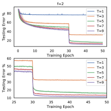
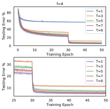
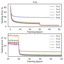
Figure 3: The testing accuracy for different frame sizes $f$ and time horizons $T$ versus the number of training epochs.

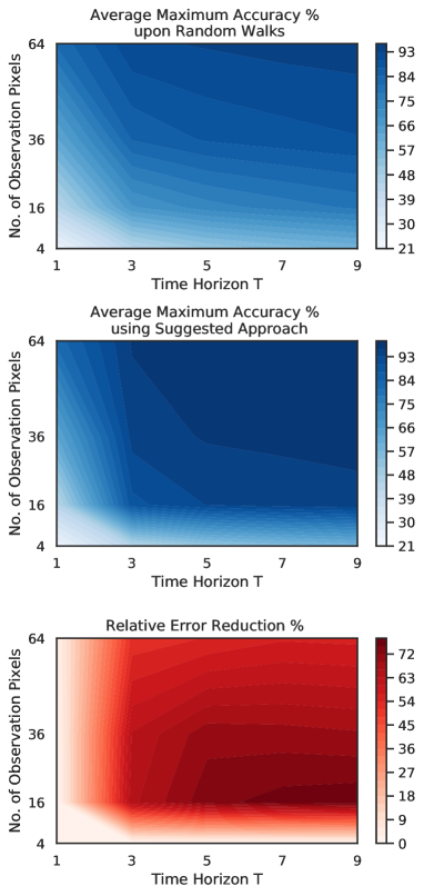
Figure 4: Average maximum testing accuracy versus frame size $f$ and time horizon $T$ after $30$ epochs with random walks (top figure). In the middle one, we trained extra $20$ training epochs for the motion planning policy. The last figure illustrates the error reduction as a result of the design of coordination policy instead of random walks.

We use the MNIST dataset of handwritten digits [20] to test the proposed learning algorithm. The dataset consists of 60,000 training images and 10,000 testing images, where each image has $28\times 28$ pixels. We suppose that each agent may observe a portion of the image that has $f\times f$ pixels. The spatial variable $p_{i}$ is the pixel coordinate of the top left corner of the observation window. The possible movements by each agent can be characterized by

$$\mathcal{A}=\{\text{up},\text{down},\text{left},\text{right}\}.$$ (24)

By each movement, the agent is translated in the desired direction by $f_{m}$ pixels. If the sampled action is infeasible, then the agent remains at its location at that time instant. In Fig. 1, as an example, we have illustrated an image from these data and the observations that three agents receive during the horizon. In all experiments of this section, we choose a mini-batches to have $64$ images during the training. We also choose the variable size of LSTM unit to be $n=64$, the number of neurons of all fully connected layers to be $64$, and the dimension of the broadcasted messages to be $n_{m}=12$. We have implemented this approach using the machine learning framework PyTorch [21].

Testing Accuracy Results: We consider $N=2$ agents that are communicating over the only option for a strongly connected graph; i.e., graph with arc set $\mathcal{E}=\{(1,2),(2,1)\}$. We choose $N_{r}=30$ and conduct a parametric study by varying observation frame size $f$ and time horizon $T$ according to $f\in\{2,4,\dots,8\}$ and $T\in\{1,3,\dots,9\}$, respectively. For each pair of $f$ and $T$, we train the model for $50$ epochs. However, we break down the training into two stages: first, we consider random walks for $30$ epochs. Then, we fix all of the parameters except for the decision-making module and train the model for another $20$ epochs. In Fig. 3, we demonstrate the progress of the testing error versus the number of training epochs. Also, in Fig. 4, we show the average maximum testing accuracy for each pair of frame size $f$ and time horizon $T$ in the case of random walks (i.e., at the end of $30$ epochs) and also with the designed law for the movements of the agents (i.e., after additional 20 epochs of training for motion planning). The results suggest that following a policy that governs the actions of the agents may significantly decrease the testing error; for instance, Fig. 5 implies that for $f=4$ (i.e., 16 observation pixels) and $T=7$ communication and observation steps, the testing error has decreased by more than $70\%$.

Remark 1

The intuition behind our two-stage method of training is that we initially train the perception, communication, and prediction modules while agents are learning to explore the environment. Once these modules are sufficiently trained, we let the agents learn how to traverse the image. The numerical experiments suggest that this training strategy generally results in smaller testing errors, compared to the case in which we simultaneously optimize the parameters of all modules. One possible justification for this observation is that the two-stage training is less prone to getting stuck in local non-stationary solutions due to higher exploration in the first phase.

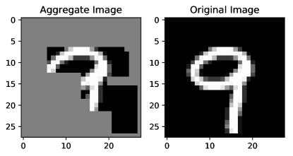
Figure 5: A sample of masked images created by putting together the observations by $3$ different agents for a time horizon of $T=3$ with $f=8$. This image is the input to the centralized image classifier as an alternative classification approach (method (i)). The (random) uncovered parts have been reached due to random walks.

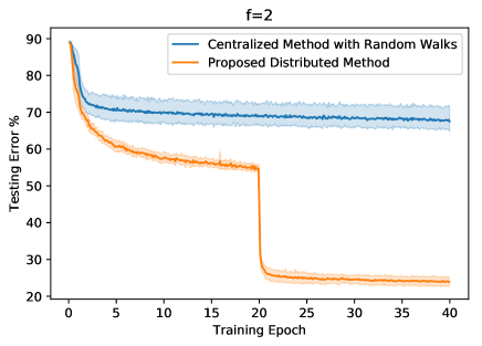
Figure 6: Comparison of the testing error when using a centralized method with the suggested approach. The first $20$ epochs of training corresponds to the case for random walks, while in the next $20$ epochs we optimize the movements of the agents.

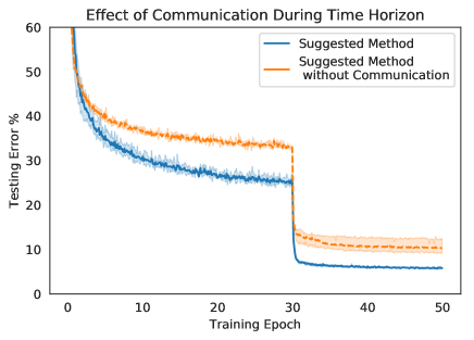
Figure 7: The result of training with and without communications.

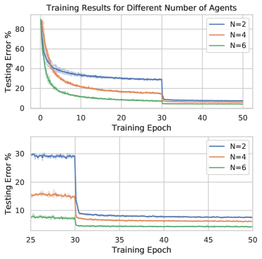
Figure 8: The training results for different number of agents.

Alternative Classification Schemes: We consider two alternative methods to classify the images based on similar observations, which will be compared against our approach. In both cases, each agent independently conducts a random walk. (i) Centralized Classification with Random Walks: we collect all the images from all agents based on random movements that have equal probability in each of four directions (i.e. $1/4$). Then, we feed the resulting unmasked image to a single CNN which is embedded into a prediction vector $q\in\mathbb{R}^{M}$ (similar to $\bar{q}$ in (13)). In Fig. 5, we demonstrate a typical input of this simple centralized classification, which has the same dimensions as the images in MNIST (i.e., $f=28$). (ii) Distributed Classification with Random Walks: We also consider a variant of Algorithm 1 in which instead of learning the optimal distributions for the policy, all possible actions in (24) have an equal probability of $1/4$. We set the parameters to $f=2$, $N=2$ agents, $N_{r}=10$ samples, time horizon $T=4$, and a complete communication graph. We conduct the training with random walks for $20$ epochs, which is followed by training of the decision-making motion planning module for another $20$ epochs. We train the centralized classification for $40$ epochs as well. In Fig. 6, we illustrate the results, which show that the quality of prediction using the proposed method is superior to both cases.

Remark 2

The main reason for which the performance of the centralized method is not better than our approach is that the masks created by random motion of the agents are not optimal.

Effect of Communication: We compare the result of training for an alternative structure in which the agents do not communicate during the horizon (although, they finally do so conduct the prediction). We set the parameters to be $N=2$, $f=4$, $N_{r}=40$, and $T=6$. As shown in Fig. 7, it turns out that smaller testing errors compared to the case that the agents do not communicate.

Effect of Number of Agents: We consider the set of parameters $f=4$, $N_{r}=25$, and $T=4$ and conduct the training for a different number of agents communicating over a complete directed graph. In Fig. 8, we illustrate the result of training for $30$ epochs with random walks followed by learning the moving policies for $20$ epochs. As expected, we observe that increasing the number of agents significantly reduces the testing error.

Visualization of Communicated Messages: We explore the patterns in the messages that are broadcasted by the agents using the learned communication medium. The goal is to visualize how the agents express the shared memory within an episode for solving the task. After training, we simulated 500 sample trajectories with $T=9$ and recorded the messages of all agents at every $t=0,\dots,8$. Then, we used the dimensionality reduction technique called t-SNE [22] to produce meaningful visualizations of the messages. In Fig. LABEL:fig:, we illustrate two t-SNE plots for the messages at $t=0$ and $t=6$, which correspond to the messages before any communication and after a few rounds of communication and observation, respectively. In these figures, every message, which is initially in $\mathbb{R}^{12}$, is reduced to a vector in $\mathbb{R}^{2}$ and is illustrated with a color corresponding to the true label of the image. The result of clustering at $t=0$ implies that initially, there is no meaningful pattern in the distribution of the labels. However, as the agents move across the image and communicate, they construct an internal belief about the true category. The second figure shows a t-SNE plot after 6 time-steps, which suggests that agents’ beliefs are reflected in the communicated messages. In fact, we observe that the digits are now clearly clustered in their own groups; i.e., they have learned to broadcast their beliefs about the true labels to their neighboring agents.

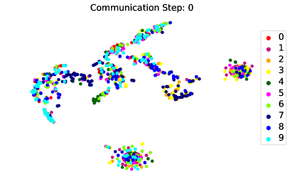
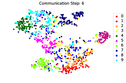
Figure 9: Visualization of the learned communications strategies and how they share their beliefs with each other using t-SNE plots.

Video: We have created a video describing our framework as well as the results of our experiments:

https://youtu.be/j67sy8RK_A4

VIII Concluding Remarks

We introduce and analyze a multi-agent image classification framework using a generalized policy gradient as the core reinforcement learning technique. The underlying ideas that are discussed in this paper are applicable to the other value-based, policy-based, or while using novel variance reduction techniques [23]. The problem studied in this paper has a discrete action space within a typically short time horizon. Depending on the problem structure (e.g., in aerial robotic applications), one may prefer a continuous action space. Then, it is straightforward to generalize our methodology to deal with these policies within this framework; for instance, using Gaussian policies [24].

Our extensive simulations suggest that the current models are temporally robust: if we train a model for time horizon $T=T_{1}$ and execute the model for $T=T_{2}>T_{1}$, the prediction quality using the second model will remain high. Also, changing the number of agents will not result in dramatic performance degradation. For example, a model trained with $3$ agents will still produce acceptable outcomes for problems with $2$ or $4$ agents. Due to space limitations, we have not included the related numerical experiments.

Our numerical experiments have been limited to $2$-D image classification. However, this framework can be applied, with minor adjustments, to more realistic scenarios. For instance, as explained in Example 3, the current framework allows the classification of $3$-D objects using a sequence of intelligently chosen $2$-D observations conducted by moving agents. The optimal (stochastic) movement of the agents around the object could be potentially related to the next best view problem [25]. Moreover, we expect that the sample efficiency of our methodology can be potentially enhanced by incorporating the developed optimal movement theories (e.g., see [26]). It is also an interesting line of research to study the cases where the graph structure dynamically (e.g. randomly) evolves over time.

References

- [1] M. A. K. Bahrin, M. F. Othman, N. H. N. Azli, and M. F. Talib, “Industry 4.0: A review on industrial automation and robotic,” Jurnal Teknologi, vol. 78, no. 6-13, 2016.
- [2] L. Yushi, J. Fei, and Y. Hui, “Study on application modes of military internet of things (miot),” in 2012 IEEE International Conference on Computer Science and Automation Engineering (CSAE), vol. 3. IEEE, 2012, pp. 630–634.
- [3] C. Bhatt, N. Dey, and A. S. Ashour, Internet of things and big data technologies for next generation healthcare. Springer, 2017, vol. 23.
- [4] R. Lowe, Y. Wu, A. Tamar, J. Harb, O. P. Abbeel, and I. Mordatch, “Multi-agent actor-critic for mixed cooperative-competitive environments,” in Advances in Neural Information Processing Systems, 2017, pp. 6379–6390.
- [5] K. Zhang, Z. Yang, H. Liu, T. Zhang, and T. Başar, “Fully decentralized multi-agent reinforcement learning with networked agents,” arXiv preprint arXiv:1802.08757, 2018.
- [6] A. Khan, C. Zhang, V. Kumar, and A. Ribeiro, “Collaborative multiagent reinforcement learning in homogeneous swarms,” 2018.
- [7] D. Silver, L. Newnham, D. Barker, S. Weller, and J. McFall, “Concurrent reinforcement learning from customer interactions,” in International Conference on Machine Learning, 2013, pp. 924–932.
- [8] H. B. McMahan, E. Moore, D. Ramage, S. Hampson et al., “Communication-efficient learning of deep networks from decentralized data,” arXiv preprint arXiv:1602.05629, 2016.
- [9] K. Bonawitz, V. Ivanov, B. Kreuter, A. Marcedone, H. B. McMahan, S. Patel, D. Ramage, A. Segal, and K. Seth, “Practical secure aggregation for privacy-preserving machine learning,” in Proceedings of the 2017 ACM SIGSAC Conference on Computer and Communications Security. ACM, 2017, pp. 1175–1191.
- [10] K. Bonawitz, H. Eichner, W. Grieskamp, D. Huba, A. Ingerman, V. Ivanov, C. Kiddon, J. Konecny, S. Mazzocchi, H. B. McMahan et al., “Towards federated learning at scale: System design,” arXiv preprint arXiv:1902.01046, 2019.
- [11] J. Foerster, I. A. Assael, N. de Freitas, and S. Whiteson, “Learning to communicate with deep multi-agent reinforcement learning,” in Advances in Neural Information Processing Systems, 2016, pp. 2137–2145.
- [12] J. N. Foerster, G. Farquhar, T. Afouras, N. Nardelli, and S. Whiteson, “Counterfactual multi-agent policy gradients,” in Thirty-Second AAAI Conference on Artificial Intelligence, 2018.
- [13] T. Nguyen and S. Mukhopadhyay, “Selectively decentralized q-learning,” in 2017 IEEE International Conference on Systems, Man, and Cybernetics (SMC). IEEE, 2017, pp. 328–333.
- [14] M. Fazel, R. Ge, S. M. Kakade, and M. Mesbahi, “Global convergence of policy gradient methods for linearized control problems,” 2018.
- [15] S. Alemzadeh and M. Mesbahi, “Distributed q-learning for dynamically decoupled systems,” arXiv preprint arXiv:1809.08745, 2018.
- [16] S. Hochreiter and J. Schmidhuber, “Long short-term memory,” Neural computation, vol. 9, no. 8, pp. 1735–1780, 1997.
- [17] I. Goodfellow, Y. Bengio, and A. Courville, Deep learning. MIT press, 2016.
- [18] A. D. Domínguez-García and C. N. Hadjicostis, “Distributed strategies for average consensus in directed graphs,” in 2011 50th IEEE Conference on Decision and Control and European Control Conference. IEEE, 2011, pp. 2124–2129.
- [19] R. S. Sutton, D. A. McAllester, S. P. Singh, and Y. Mansour, “Policy gradient methods for reinforcement learning with function approximation,” in Advances in neural information processing systems, 2000, pp. 1057–1063.
- [20] Y. LeCun, L. Bottou, Y. Bengio, and P. Haffner, “Gradient-based learning applied to document recognition,” Proceedings of the IEEE, vol. 86, no. 11, pp. 2278–2324, 1998.
- [21] A. Paszke, S. Gross, S. Chintala, G. Chanan, E. Yang, Z. DeVito, Z. Lin, A. Desmaison, L. Antiga, and A. Lerer, “Automatic differentiation in pytorch,” in NIPS-W, 2017.
- [22] L. v. d. Maaten and G. Hinton, “Visualizing data using t-sne,” Journal of machine learning research, vol. 9, no. Nov, pp. 2579–2605, 2008.
- [23] R. Johnson and T. Zhang, “Accelerating stochastic gradient descent using predictive variance reduction,” in Advances in neural information processing systems, 2013, pp. 315–323.
- [24] T. Zhang, G. Kahn, S. Levine, and P. Abbeel, “Learning deep control policies for autonomous aerial vehicles with mpc-guided policy search,” in 2016 IEEE international conference on robotics and automation (ICRA). IEEE, 2016, pp. 528–535.
- [25] C. Connolly, “The determination of next best views,” in Proceedings. 1985 IEEE International Conference on Robotics and Automation, vol. 2. IEEE, 1985, pp. 432–435.
- [26] C. Esteves, C. Allen-Blanchette, A. Makadia, and K. Daniilidis, “Learning so (3) equivariant representations with spherical cnns,” in Proceedings of the European Conference on Computer Vision (ECCV), 2018, pp. 52–68.