A Variational Approach to Sparse Model Error Estimation in Cardiac Electrophysiological Imaging

Abstract

Noninvasive reconstruction of cardiac electrical activity from surface electrocardiograms (ECG) involves solving an ill-posed inverse problem. Cardiac electrophysiological (EP) models have been used as important a priori knowledge to constrain this inverse problem. However, the reconstruction suffer from inaccuracy and uncertainty of the prior model itself which could be mitigated by estimating a priori model error. Unfortunately, due to the need to handle an additional large number of unknowns in a problem that already suffers from ill-posedness, model error estimation remains an unresolved challenge. In this paper, we address this issue by modeling and estimating the a priori model error in a low dimensional space using a novel sparse prior based on the variational approximation of L0 norm. This prior is used in a posterior regularized Bayesian formulation to quantify the error in a priori EP model during the reconstruction of transmural action potential from ECG data. Through synthetic and real-data experiments, we demonstrate the ability of the presented method to timely capture a priori model error and thus to improve reconstruction accuracy compared to approaches without model error correction.

1 Introduction

Noninvasive electrophysiological (EP) imaging aims at a mathematical and computational reconstruction of cardiac sources from high density electrocardiogram (ECG) signals. It requires solving an inverse problem with severe ill-posedness, especially when cardiac sources are solved transmurally throughout the 3D myocardium. To overcome this challenge, an important approach is to incorporate a constraining model encoding a priori physiological knowledge about the electrical activity inside the heart. Examples of such models include simple step jump functions [9] to describe the activation of action potential, parameterized curve models to describe the spatiotemporal wavefront evolution [5], and biophysical EP models to describe the dynamics of action potential via differential equations [6, 10]. While the use of such a priori models is effective in regularizing the ill-posed problem, often the inaccuracy and uncertainty of the model itself creates errors and uncertainty in the solution [4]. This issue of model inaccuracy and the resulting solution uncertainty has been studied with convex relaxation of the original problem of EP imaging [4]. Similarly, uncertainty in the inverse solution of EP imaging due to model error, and its consideration to improve the clinical interpretation was explored in [11]. While these works have highlighted the importance of model error in EP imaging, addressing these errors when the prior knowledge is in the form of a complex physiological model remains a challenge.

Outside EP imaging, the issue of error and uncertainty in model prediction has been an active area of research in weather and climate forecasting. One common approach is to model the error as a zero-mean Gaussian distribution with an unknown covariance to be inferred from data. To address high dimensionality, the covariance matrix is usually parameterized by a small set of parameters, such as via a linear combination of basis matrices weighted by parameters to be learned from data [3]. Another common approach is to model the error, for example as a function of error in model parameters [7]. In either case, the key is to exploit the prior knowledge about the nature of the error to reduce dimension.

In this paper, we exploit the low-dimensional nature of cardiac wavefront propagation to formulate a sparse model for the prediction error made by a a priori EP model. Wavefront, which can be thought as the spatial gradient of action potential, is always localized in a small region at a time. This provides the motivation to focus on the model inaccuracy in the spatial gradient (i.e., error of the predicted wavefront), which will reduce the dimension of the unknown error while preserving the accuracy of the low-dimensional representation of the inverse solution. To do so, we present a posterior regularized Bayesian approach to the reconstruction of transmural action potential from ECG data, in which a generalized Gaussian distribution is formulated to model the sparse error in the gradient domain. A variational lower bound of the generalized Gaussian distribution is derived, based on which we quantify the model error while simultaneously reconstructing the action potential. As we will show mathematically, solution of the inference problem will amount to iteratively estimating the prior covariance matrix of the predicted action potential, such that the condition of sparsity in error is satisfied. In both synthetic and real-data experiments, we demonstrate the ability of the presented method to timely capture the prediction error in the a priori EP model, and thereby to deliver more accurate reconstructions of action potential compared to approaches without model error correction.

2 Bayesian Formulation with Error Modeling

The relation between ECG and transmural action potential can be described by a quasi-static approximation of the Maxwell’s equations for an electromagnetic field [10]. Solving these equations numerically on a subject-specific heart-torso model, a linear forward model can be obtained as $\textbf{y}_{k}=\textbf{H}\textbf{u}_{k}$, where H is called the forward matrix, and $\textbf{y}_{k}$ and $\textbf{u}_{k}$ respectively denote a vector of ECG and action potential at any time instant $k$. The inverse problem constitutes the estimation of $\textbf{u}_{k}$ given data $\textbf{y}_{k}$ for all time $k$.

One of the important constraints used to regularize the ill-posed inverse problem of ECG is the cardiac EP model describing the spatiotemporal propagation of the action potential inside the heart [6, 10]. Assuming that the temporal evolution of the action potential follows a markov model, the action potential at every time instant $k$ can be predicted from its value at the previous time instant using the a priori EP model. Without the loss of generality, the two-variable Aliev-Panfilov model [1] is adopted in this paper for this purpose. We drop subscript k for clarity for the rest of the paper.

One common way to calculate the posterior distribution of u is to apply Bayes theorem as $p(\textbf{u}|\textbf{u}_{prev},\textbf{y})={p(\textbf{y}|\textbf{u})p(\textbf{u}|\textbf{u}_{prev})}/{p(\textbf{y})}$, where $\textbf{u}_{prev}$ is the estimated action potential at previous time instant. In addition, we are also interested in calculating posterior distribution of u such that the value of u is constrained within its physiological range, i.e.,$-90mV\leq\textbf{u}\leq 20mV$. This is achieved by finding a distribution $r(\textbf{u})$ which minimizes the Kullback-Leibler(KL) divergence $\textrm{KL}(r(\textbf{u})||p(\textbf{u}|\textbf{u}_{prev},\textbf{y}))$ from $r(\textbf{u})$ to $p(\textbf{u}|\textbf{u}_{prev},\textbf{y})$. This is equivalent to finding an optimum solution of following convex problem [12]:

$$p(\textbf{u}|\textbf{y},\textbf{u}_{prev}) =\underset{r(u)}{\min}\hskip 8.5359pt\textrm{KL}(r(\textbf{u})||p(\textbf{u}|\textbf{u}_{prev}))-\int_{\textbf{u}}{r(\textbf{u})\log p(\textbf{y}|\textbf{u})d\textbf{u}}$$

$$s.t.\hskip 8.5359ptr(\textbf{u})\in\mathcal{P}_{post}$$ (1)

where $\mathcal{P}_{post}$ denotes the subspace of Gaussian distributions whose mean lie in the range [-90mV,20mV].

2.0.1 Likelihood Function:

The forward model is incorporated in the likelihood function given by $p(\textbf{y}|\textbf{u},\beta)=\mathcal{N}(\textbf{y}|\textbf{Hu},\beta^{-1}\textbf{I})$ where $\beta^{-1}$ denotes the unknown variance of data error and the inverse variance, $\beta$, follows a Gamma distribution.

2.0.2 Prior Distribution with Error Modeling:

The prediction from the a priori EP model is incorporated into a prior distribution on u.

$$\textbf{u}=\textbf{u}_{pd}+\tilde{\boldsymbol{\eta}}= \bar{\textbf{u}}_{pd}+\mathcal{N}(0,\textbf{C}_{pd})+\tilde{\boldsymbol{\eta}}$$ (2)

$$= \bar{\textbf{u}}_{pd}+\boldsymbol{\eta}$$ (3)

where $\textbf{u}_{pd}=f(\textbf{u}_{prev})$ represents the distribution predicted by EP model, $f(\cdot)$ represent the corresponding function and $\tilde{\boldsymbol{\eta}}$ represents model error . Because $f(\cdot)$ is nonlinear, $\textbf{u}_{pd}$ is calculated by taking a set of samples from the estimated posterior distribution of $\textbf{u}_{prev}$, passing them through the EP model, and fitting a Gaussian distribution to the output samples. In most existing works that use such a model to constrain the reconstruction of u, $\tilde{\boldsymbol{\eta}}$ is assumed to be a zero-mean Gaussian error with a known covariance that is experimentally adjusted for sub-optimal reconstruction accuracy [10]. In our case, we absorb all the uncertainties into error vector $\boldsymbol{\eta}=\mathcal{N}(0,\textbf{C}_{pd})+\tilde{\boldsymbol{\eta}}$. To directly estimate $\boldsymbol{\eta}$, however, will translate to the estimation of a high-dimensional covariance matrix that is infeasible given the limited ECG data. We address this problem by modeling the prediction error $\boldsymbol{\eta}$ to be sparse in the spatial gradient domain, utilizing the knowledge about the spatial sparsity of the action potential wavefront. Let D denote a spatial gradient operator on the cardiac mesh, we denote the error in the gradient domain as $\textbf{x}=\textbf{D}\boldsymbol{\eta}$.

In deterministic cases in the field of compressed sensing [2], it has been shown that a Lp-norm constraint with $0<p<1$ can be used to promote sparsity, where the sparsity increases as p decreases towards 0. In order to use the same concept in a probabilistic setting, we propose a generalized Gaussian distribution as a prior distribution over variable x, with the value of $p\approx 0$ to approximate the effect of a L0 norm constraint:

$$p_{\textbf{x}}(\textbf{x}|\alpha) =\prod_{i}\frac{C}{\alpha}\exp(\frac{-\lvert x_{i}\rvert^{p}}{\alpha^{p}})$$ (4)

where $x_{i},i=1,\cdots,N$ are independent elements in the vector x, $\alpha$ is the parameter of distribution and $C$ is normalization constant. The prior distribution of u can then be obtained by replacing $\textbf{x}=\textbf{D}\boldsymbol{\eta}=\textbf{D}(\textbf{u}-\bar{\textbf{u}}_{pd})$ in eq.(4):

$$p(\textbf{u}|\bar{\textbf{u}}_{pd})\propto{p_{\textbf{x}}(\textbf{D}(\textbf{u}-\bar{\textbf{u}}_{pd}))}$$ (5)

3 Posterior Regularized Bayes for EP Imaging

3.0.1 Variational Lower Bound:

The posterior distribution in equation (2) is analytically intractable given the generalized Gaussian prior as defined in equation (5) due to presence of absolute value in the exponent. Below we present a solution strategy based on its variational lower bound.

Lemma 1

$\exp(\frac{-\lvert x\rvert^{p}}{\alpha^{p}})\geq\exp\left(-\frac{x^{2}}{2\tau}-\frac{2-p}{2}(\frac{\alpha^{2}}{p\tau})^{\frac{p}{p-2}}\right),\hskip 0.28436pt\forall\tau>0,x\in\bbbr,\alpha>0$ [8]

Theorem 3.1

Let $\textbf{x}=(x_{1},x_{2},...x_{N})$ be a vector with independent components each following a generalized normal distribution with same parameters $\alpha,p$. then,

$$p(\textbf{x}|\alpha)\geq\frac{C^{\prime}}{\alpha^{N}}\exp(-\frac{\textbf{x}^{T}\textbf{Ax}}{2})\exp\left(-\frac{2-p}{2}(\frac{\alpha^{2}}{p})^{\frac{p}{p-2}}\sum_{i}\lambda_{i}^{\frac{p}{p-2}}\right)$$

Proof

Using Lemma 1 in prior distribution as defined in eq.(4), we have

$$p(\textbf{x}|\alpha) \geq\frac{C^{\prime}}{\alpha^{N}}\exp(-\sum_{i}\frac{x_{i}^{2}}{2\tau_{i}})\exp\left(-\sum_{i}\frac{2-p}{2}(\frac{\alpha^{2}}{p\tau_{i}})^{\frac{p}{p-2}}\right)$$ (6)

$$=\frac{C^{\prime}}{\alpha^{N}}\exp(-\frac{\textbf{x}^{T}\textbf{Ax}}{2})\exp\left(-\frac{2-p}{2}(\frac{\alpha^{2}}{p})^{\frac{p}{p-2}}\sum_{i}\lambda_{i}^{\frac{p}{p-2}}\right)$$ (7)

where $\textbf{A}=diag(\boldsymbol{\lambda})$, $C^{\prime}=C^{N}$, and $\lambda=\tau^{-1}$ is used in eq.(7) ∎

Theorem 1 gives us a variational lower bound for the generalized Gaussian distribution defined in equation (4). Applying it to equation (5), we obtain a variational lower bound for the prior distribution of $p(\textbf{u}|\textbf{u}_{pd})$ as follows:

$$p(\textbf{u}|\bar{\textbf{u}}_{pd}) \geq q(\textbf{u}|\bar{\textbf{u}}_{pd},\boldsymbol{\lambda},\alpha)$$

$$\propto \frac{C^{\prime}}{\alpha^{N}}\exp(\frac{-(\textbf{u}-\bar{\textbf{u}}_{pd})^{T}\textbf{D}^{T}\textbf{AD}(\textbf{u}-\bar{\textbf{u}}_{pd})}{2}-\frac{2-p}{2}(\frac{\alpha^{2}}{p})^{\frac{p}{p-2}}\sum_{i}\lambda_{i}^{\frac{p}{p-2}})\normalsize$$

3.0.2 Inference:

The posterior distribution in equation (2) can now be solved by maximizing the variational parameters of prior distribution as defined in eq.(3.0.1). It is achieved by following two steps: 1) estimate parameters $\boldsymbol{\lambda},\alpha$ and $\beta$ by Expectation Maximization (EM), and 2) obtain the posterior distribution of u by posterior regularized Bayes [12].

Parameters $\boldsymbol{\lambda},\alpha$ and $\beta$ are estimated using EM by marginalizing over hidden variable u where the two steps : E step and M step are iterated until convergence. In the E-step, we take expectation and obtain a function $\mathcal{L}$ as

$$\mathcal{L}(\alpha,\beta,\boldsymbol{\lambda})=E_{q(\textbf{u})}[log\left(p(\textbf{u,y}|\alpha,\boldsymbol{\lambda},\beta)\right)+log(\beta)]$$ (9)

where $E_{q(\textbf{u})}[\hskip 2.84544pt]$ denotes the expectation with respect to the posterior distribution of u with fixed parameters $\boldsymbol{\alpha}_{old},\boldsymbol{\beta}_{old},\boldsymbol{\lambda}_{old}$ obtained in previous iteration. The M-step consists of the following maximization:

$$\alpha_{new},\beta_{new},\boldsymbol{\lambda}_{new} =\underset{\alpha,\beta,\boldsymbol{\lambda}}{argmax}\hskip 14.22636pt\mathcal{L}(\alpha,\beta,\boldsymbol{\lambda})$$ (10)

It is noteworthy that for fixed values of parameters, the prior distribution as defined in equation (3.0.1) is Gaussian with the covariance matrix $\textbf{(D}^{T}\textbf{AD)}^{-1}$ and $\textbf{A}=diag(\boldsymbol{\lambda})$. This gives an interesting interpretation of the presented EM procedure as an iterative process to estimate the prior covariance matrix. In specific, if we focus on the wavefront Du, the diagonal element of the matrix $\textbf{A}^{-1}$ describes the variance of each individual element in Du. We will show in section 4 how this estimated variance is related to the a priori model error.

Once the values of parameters $\hat{\alpha},\hat{\beta},\hat{\boldsymbol{\lambda}}$ are obtained by the EM procedure, $\hat{\boldsymbol{\lambda}},\hat{\alpha}$ are plugged in eq.(3.0.1) to obtain prior distribution $q(\textbf{u}|\bar{\textbf{u}}_{pd},\hat{\boldsymbol{\lambda}},\hat{\alpha},)$ which is then used in eq.(2) to obtain posterior distribution . Since a Gaussian distribution is specified by mean and covariance, the minimization of (2) is done over a space of mean vectors and covariance matrices satisfying the given constraints.

4 Results

While we described a general algorithm for model error estimation, we test it for the detection of errors in a priori EP model due to the presence of myocardial scar tissue. Using synthetic and real data experiments, we compare the performance of the proposed method to that without model error estimation [10]

4.0.1 Synthetic Experiments:

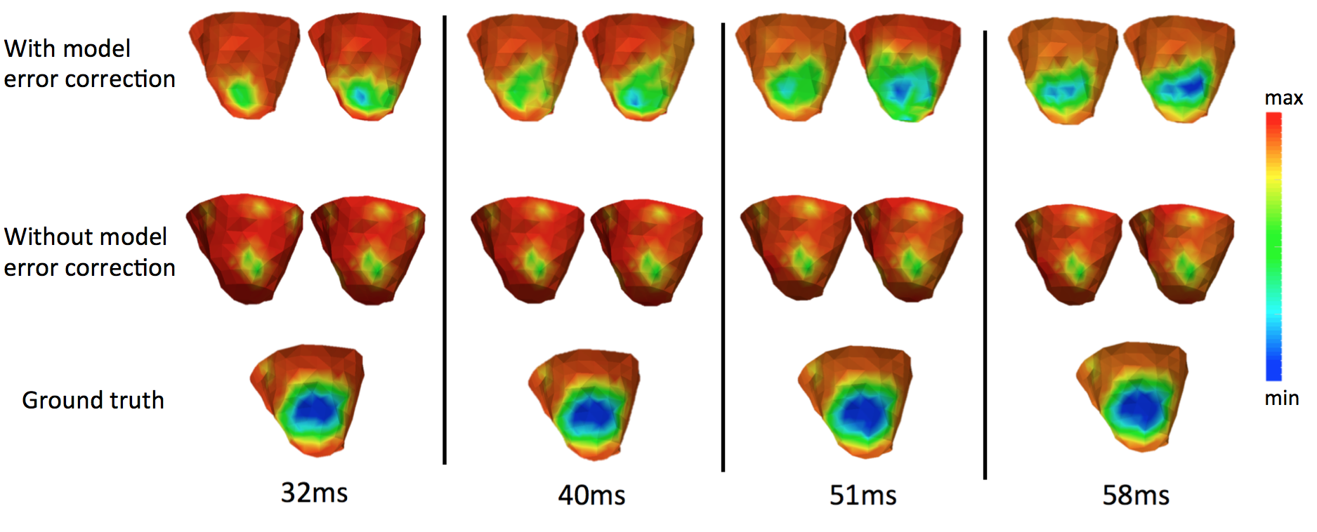
Figure 1: Snapshots of the action potential at different time instants. For each method at each time instant, the figure on the left shows the prediction from the a priori EP model; the figure on the right shows the estimated result.

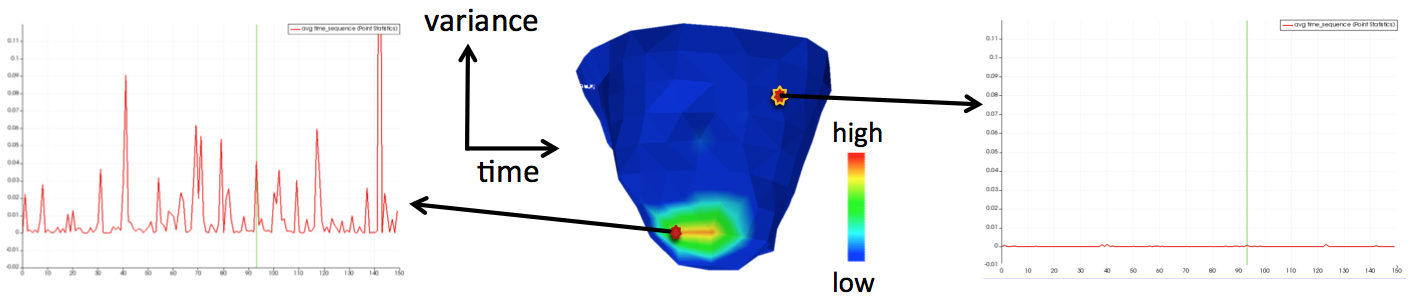
Figure 2: Centre shows spatial map of variance at various locations of the heart at a time. Two sides show temporal plots of the estimated variance at a site of scar tissue (left) and healthy tissue (right)

We test our method in a set of 17 experiments on image-derived heart-torso models with the myocardial scar set according to the AHA 17-segment model of the LV. 120-lead ECG data are simulated and corrupted with 20 dB Gaussian noise for inverse reconstruction. From the reconstructed action potential, activation time is extracted and scar is identified as the regions with an activation time larger than a threshold value. The accuracy of the detected scar is measured with two metrics: a) dice coefficient=2($S_{1}\cap S_{2}$)/($S_{1}\cup S_{2}$), where $S_{1}$ and $S_{2}$ are reconstructed and true regions of scar, b) distance from the reconstructed center to actual center of scar.

Fig. 1 gives an example where a myocardial scar is located towards the anterior base of the LV. The a priori EP model, however, assumes normal tissue property throughout the myocardium. As a result, model error exists in the predictions made by the EP model once the action potential propagates through the region of the myocardial scar. Compared to the method without model error correction, the proposed method is able to make significant improvements in two fronts: 1) the presented method corrects model errors significantly to drive the solution closer to the ground truth at each time instant, and 2) the reconstructed solution is corrected toward the ground truth much earlier in time. As shown in Fig. 2, higher variance of the wavefront is obtained at the region near myocardial scar, signifying possible errors in the model at those regions of the wavefront. This increase in prior variance of wavefront helps make significant data-driven correction to the a priori prediction. The temporal trace of the variance also shows that the estimated variance is consistently higher around the scar than that around the healthy tissue, suggesting low model errors in the latter region.

Fig. 3b lists the quantitative accuracy of the detected scar with and without model error estimation, where a statistically significant improvement of accuracy is obtained with model error estimation (unpaired-t tests, p$<$0.005). Note that, Without error estimation, late activation due to scar is not captured in 50% of the cases, and the metrics are calculated only from those where late activation is successfully reconstructed. Several examples of the reconstructed activation time are shown in Fig. 3a, demonstrating the improvement of the delayed activation reconstructed at the region of myocardial scar by the presented method.

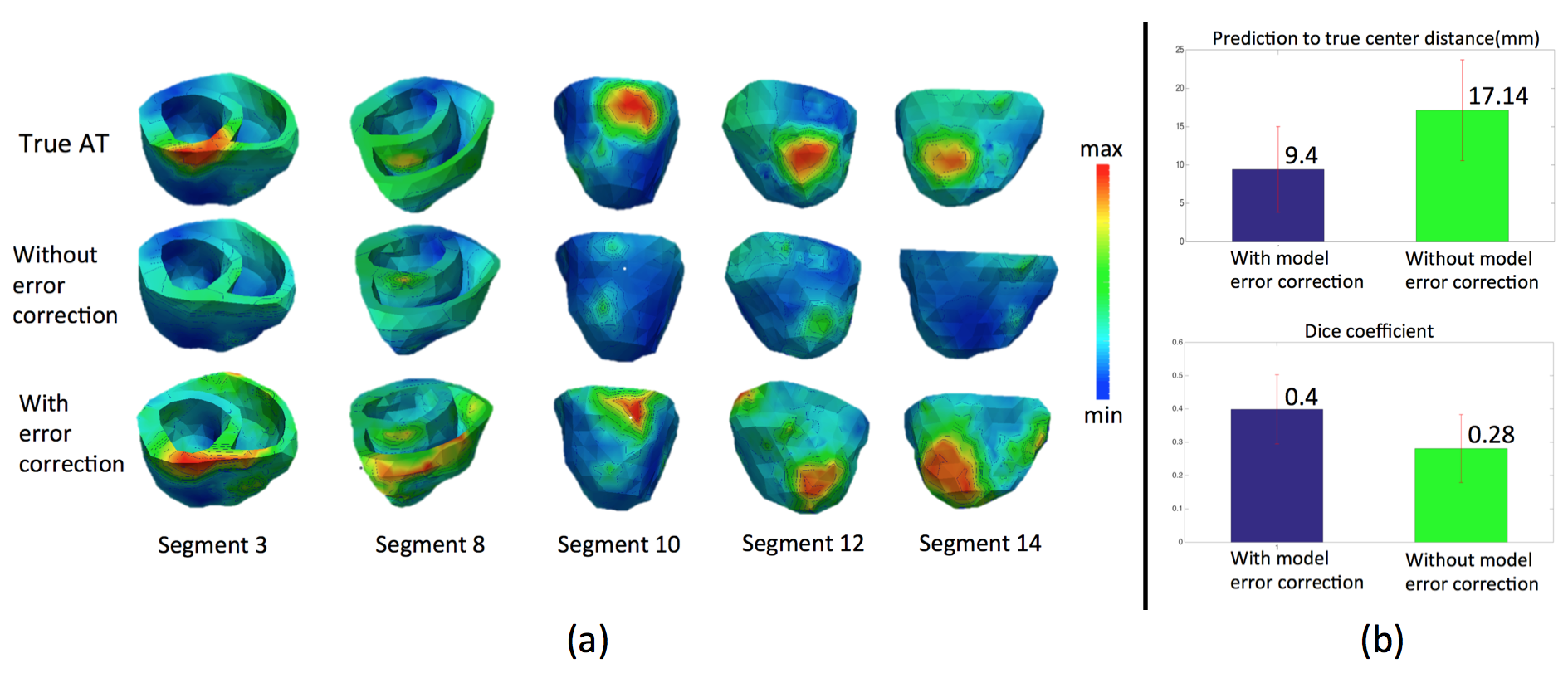
Figure 3: a) Activation time maps. Regions with high values of activation time correspond to regions of scar. b) Comparison of the accuracy of scar detection with and without model error correction.

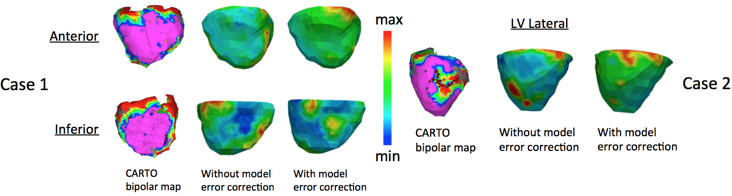
Figure 4: Real data results of activation time maps versus in-vivo bipolar voltage maps. In bipolar voltage maps, red regions correspond to scar and purple regions correspond to healthy tissue. In the reconstructed activation time maps, regions of high activation time correspond to scar.

4.0.2 Real-data Experiment:

Two real-data case studies are performed on patients who underwent catheter ablation due to scar-related ventricular arrhythmia. From 120-lead ECG data, action potential is reconstructed with and without model error estimation. Bipolar voltage data from in-vivo catheter mapping is used as reference to evaluate the detected scar regions. As shown in Fig. 4, in Case 1, the presented method with model error correction is able to identify the area of scar at both the anterior and inferior base. In contrast, reconstruction without error correction is only able to find scar in the inferior basal region. For Case 2, results from both methods are similar if one were to look at the region of high activation time (red region). However, at the mid-lateral region where voltage map shows the presence of scar, the activation time in the reconstruction with error correction is still high (green), while it is low (blue) for the reconstruction without error correction.

5 Conclusion

This paper presents a novel approach to model and estimate the error in a priori EP models by exploiting its sparsity in the gradient domain. Experiments show promising results in the ability of the presented method to timely capture the error in the a priori model at the correct spatial location. The next step would be to utilize the estimated variance to correct the model, e.g., by facilitating the estimation of its spatial parameters.

References

- [1] Aliev, R.R., Panfilov, A.V.: A simple two-variable model of cardiac excitation. Chaos, Solitons & Fractals 7(3), 293–301 (1996)
- [2] Chartrand, R., Yin, W.: Iteratively reweighted algorithms for compressive sensing. In: 2008 IEEE ICASSP. pp. 3869–3872. IEEE (2008)
- [3] Dee, D.P.: On-line estimation of error covariance parameters for atmospheric data assimilation. Monthly weather review 123(4), 1128–1145 (1995)
- [4] Erem, B., van Dam, P., Brooks, D.: Identifying model inaccuracies and solution uncertainties in non-invasive activation-based imaging of cardiac excitation using convex relaxation. IEEE TMI (99) (2014)
- [5] Ghodrati, A., Brooks, D.H., Tadmor, G., MacLeod, R.S.: Wavefront-based models for inverse electrocardiography. IEEE transactions on biomedical engineering 53(9), 1821–1831 (2006)
- [6] Nielsen, B.F., Lysaker, M., Grøttum, P.: Computing ischemic regions in the heart with the bidomain model—first steps towards validation. IEEE TMI 32(6), 1085–1096 (2013)
- [7] Onatski, A., Williams, N.: Modeling model uncertainty. Journal of the European Economic Association 1(5), 1087–1122 (2003)
- [8] Palmer, J., Wipf, D., Kreutz-Delgado, K., Rao, B.: Variational em algorithms for non-gaussian latent variable models. Advances in neural information processing systems 18, 1059 (2006)
- [9] Pullan, A., Cheng, L., Nash, M., Bradley, C., Paterson, D.: Noninvasive electrical imaging of the heart: theory and model development. Annals of biomedical engineering 29(10), 817–836 (2001)
- [10] Wang, L., Zhang, H., Wong, K.C., Liu, H., Shi, P.: Physiological-model-constrained noninvasive reconstruction of volumetric myocardial transmembrane potentials. IEEE Transactions on Biomedical Engineering 57(2), 296–315 (2010)
- [11] Xu, J., Sapp, J.L., Dehaghani, A.R., Gao, F., Wang, L.: Variational bayesian electrophysiological imaging of myocardial infarction. In: International Conference on MICCAI. pp. 529–537. Springer (2014)
- [12] Zhu, J., Chen, N., Xing, E.P.: Bayesian inference with posterior regularization and applications to infinite latent svms. JMLR 15(1), 1799–1847 (2014)