The Most Metal-Poor Stars. V. The CEMP-no Stars in 3D and Non-LTE

Abstract

We explore the nature of carbon-rich ([C/Fe]_1D,LTE $>$ +0.7), metal-poor ([Fe/H_1D,LTE] $<$ –2.0) stars in the light of post 1D,LTE literature analyses, which provide 3D–1D and NLTE–LTE corrections for iron, and 3D–1D corrections for carbon (from the CH G-band, the only indicator at lowest [Fe/H]). High-excitation C I lines are used to constrain 3D,NLTE corrections of G-band analyses. Corrections to the 1D,LTE compilations of Yoon et al. and Yong et al. yield 3D,LTE and 3D,NLTE Fe and C abundances. The number of CEMP-no stars in the Yoon et al. compilation (plus eight others) decreases from 130 (1D,LTE) to 68 (3D,LTE) and 35 (3D,NLTE). For stars with –4.5 $<$ [Fe/H] $<$ –3.0 in the compilation of Yong et al., the corresponding CEMP-no fractions change from 0.30 to 0.15 and 0.12, respectively.

We present a toy model of the coalescence of pre-stellar clouds of the two populations that followed chemical enrichment by the first zero-heavy-element stars: the C-rich, hyper-metal-poor and the C-normal, very-metal-poor populations. The model provides a reasonable first-order explanation of the distribution of the 1D,LTE abundances of CEMP-no stars in the $A$(C) and [C/Fe] vs. [Fe/H] planes, in the range –4.0 $<$ [Fe/H] $<$ –2.0.

The Yoon et al. CEMP Group I contains a subset of 19 CEMP-no stars (14% of the group), 4/9 of which are binary, and which have large [Sr/Ba]_1D,LTE values. The data support the conjectures of Hansen et al. (2016b, 2019) and Arentsen et al. (2018) that these stars may have experienced enrichment from AGB stars and/or “spinstars”.

The predicted 3D corrections for molecular lines would also alleviate the extraordinarily large C abundances found in some very metal-poor stars. … Similarly, the fraction of strongly C-enhanced ([C/Fe] $\;\buildrel>\over{\sim}\;$ +1.0) metal-poor stars is likely substantially less than the claimed $>$20% for [Fe/H] $\;\buildrel<\over{\sim}\;$ –2.0. …              – M. Asplund (2005)

1 Introduction

The CEMP-no sub-population of carbon-enhanced metal-poor (CEMP) stars, with [C/Fe] $>$ +0.7 but no enhancement of heavy neutron-capture elements, arguably contains the most chemically primitive objects currently known. Indeed, among the 12 of the 14 metal-poor stars that have [Fe/H] $<$ –4.5 and [C/Fe] $>$ +1.0, 11 have [C/Fe] $>$ +3.0, while three have values +1.6, $<$+0.9, and $<$+1.8 dex (see Tables 1 and  6 for details). At least 12 of the 14 belong to the CEMP-no group. It has been argued that the latter objects formed within a few hundred million years after the Big Bang, and probably did so before the carbon-normal stars ([C/Fe] $<$ +0.7 and [Fe/H] $\;\buildrel>\over{\sim}\;$ –4.5). Table 1 presents a list of some 23 major milestones on the nature of these objects and the role they play in our understanding of the early Universe. Figure 1 shows the dependence of the carbon abundance, $A$(C)_1D,LTE, and relative carbon abundance, [C/Fe]_1D,LTE, as a function of [Fe/H]_1D,LTE for these CEMP-no stars, together with their carbon distribution as a function of [Fe/H]_1D,LTE. For definitions, and recent reviews and introductions to the extensive literature on CEMP-no stars, we refer the reader to Beers & Christlieb (2005), Norris et al. (2013), Frebel & Norris (2015), Hansen et al. (2016b), Yoon et al. (2016), and Matsuno et al. (2017).

The data in Figure 1 are taken from the literature-based compilation of Yoon et al. (2016) in which the carbon abundances of the CEMP-no stars were determined by analysis of the G-band of the CH molecule at $\lambda$4300 Å, [Fe/H] is based essentially on Fe I lines, and model atmosphere techniques together with the almost universally adopted one dimensional (1D) and Local Thermodynamic Equilibrium (LTE) assumptions (hereafter 1D,LTE) were used. While this technique has proved very useful in the past, in particular in differential analyses based on atomic species, it is not necessarily the case for molecular features. As emphasized by Asplund and coworkers (see Asplund 2005), errors of order $\Delta$$A$(C) = –1 dex might be expected in extremely metal-poor stars as a result of the 1D assumption; and as highlighted in the above introductory quotation, one should be alive to the possibility that some of the apparent characteristics of the CEMP-no stars might result from the 1D,LTE assumptions made in the analysis, rather than the potentially more realistic 3D and non-LTE (hereafter 3D,NLTE) ones. More generally, while 1D,LTE is currently a more precise formalism than 3D,NLTE (which is a much more challenging endeavor) it is the latter that will result in more accurate results.

The aim of the present work is to use literature-based corrections determined by adopting the assumptions of 3D,NLTE to correct carbon and iron abundances based on those of 1D,LTE. The outline of the paper is as follows. In Section 2 we address semantics of carbon richness relevant to the present work. Section 3 summarizes results from the literature for 3D–1D,LTE corrections for the analysis of both the G-band and Fe I lines and 3D–1D,NLTE corrections for Fe I lines. In order to address the problem that determination of NLTE corrections is not currently possible for the CH molecule, we also use abundances from infrared high-excitation C I lines to constrain the CH NLTE corrections in the range –3.3 $<$ [Fe/H] $<$ –2.0. In Section 4 we use these corrections to update the 1D,LTE Fe and C abundances of Yoon et al. (2016), Yong et al. (2013a), and a few more recent values, to place them within the 3D,LTE and 3D,NLTE frameworks. As foreshadowed by Asplund (2005) the changes are large, and in Section 5, following Yong et al. (2013b), we address their effect on the Metallicity Distribution Function and the fraction of CEMP (principally CEMP-no) stars in the range [Fe/H] $<$ –3.0. For completeness, Section 6 discusses some uncertainties of the present work, while Section 7 addresses 1D,LTE abundances of the light elements Na, Mg, Al, and Ca, together with the heavy neutron-capture elements Sr and Ba, and their implications for the nature of the CEMP-no stars. In Section 8 we present a toy model that seeks to explain the CEMP-no stars in the abundance range –4.0 $<$ [Fe/H] $<$ –2.0 in terms of the coalescence of gas clouds of C-rich material of the second generation ([Fe/H] $<$ –5.0, [C/Fe] $\;\buildrel>\over{\sim}\;$ +1.0), and those of the C-normal stars of the canonical halo population ([Fe/H] $>$ –4.0, [C/Fe] = 0.0). Section 9 summarizes our results.

2 The Semantics of Carbon Richness

Just what does one mean by carbon richness? In almost all discussions based on the analysis of the G-band strength in the spectra of metal-poor stars with [Fe/H] $\;\buildrel<\over{\sim}\;$ –3.0, the framework is based on 1D,LTE assumptions, and a star is C-rich if it has an abundance [C/Fe]_1D,LTE $>$ +0.7 (following Beers & Christlieb, 2005 and Aoki et al., 2007). If, however, 1D,LTE-based results were to overestimate carbon abundances, by, say, 0.7 dex, stars “observed” at this limit would in reality have the solar relative carbon abundance. If one is interested in abundances relative to the sun, it thus follows there is a problem in defining an abundance limit based on a formalism that has systematic errors which are a function of chemical abundance. It would be better to choose an independent limit relative to the solar abundance that would be useful when seeking to compare stellar overabundances with, for example, overabundances that might be observed in other fields, such as gaseous nebulae and far-field cosmology, and also theoretical models of stellar, galactic, and cosmological formation and evolution.

Insofar as we shall be discussing carbon and iron abundances determined using different assumptions we adopt the following definitions. As noted above, [Fe/H]_1D,LTE and [C/Fe]_1D,LTE refer to values determined assuming 1D,LTE. [Fe/H]_3D,LTE and [C/Fe]_3D,LTE assume 3D,LTE, and [Fe/H]_3D,NLTE and [C/Fe]_3D,NLTE adopt 3D,NLTE. [Fe/H] and [C/Fe] are used generically. Finally, we adopt a generic carbon overabundance limit for all of these cases that somewhat arbitrarily defines carbon richness as [C/Fe] $>$ +0.7 as the independent limit.

3 3D and Non-LTE Corrections

In order to convert the available 1D,LTE carbon and iron abundances of very metal-poor stars to include 3D and NLTE effects, we seek corrections of the form $\Delta$$A$(X)_{3D,NLTE-1D,LTE} = $A$(X)_3D,NLTE – $A$(X)_1D,LTE for analyses of the CH G-band (X = C) and Fe lines (X = Fe). The enormous computational challenge to this requirement is highlighted by the very small number of relevant papers available in the literature. Further, in most cases, one finds partial solutions involving changes between only 3D and 1D, assuming LTE ($\Delta$$A$(X)_(3D-1D),LTE = $A$(X)_3D,LTE – $A$(X)_1D,LTE), or between only NLTE and LTE, assuming 1D ($\Delta$$A$(X)_{1D,(NLTE-LTE)} = $A$(X)_1D,NLTE – $A$(X)_1D,LTE). As noted above, in the case of carbon abundances determined from analysis of the CH G-band, NLTE corrections are not currently possible. To cite Gallagher et al. (2016) “computing full 3D … NLTE … departures for molecular data … has not been attempted in great detail because of the complexities involved”.

With this in mind we first discuss what is currently possible in the analysis of the G-band, together with results for Fe I lines. Following this, we consider the analysis of near-infrared high-excitation C I lines in metal-poor stars, in order to place constraints on the role of NLTE in determining $A$(C)_3D,NLTE values based on analysis of the G-band.

3.1 3D and NLTE corrections for the G-band and Fe I lines

Literature information that we shall use is presented in Table 2, where Columns (1) – (3) contain the star or model name, $T_{\rm eff}$, and $\log g$, respectively, while Columns (4) – (9) present [Fe/H]_1D,LTE, [Fe/H]_1D,NLTE, [Fe/H]_3D,LTE, [Fe/H]_3D,NLTE, $A$(C)_1D,LTE, and $A$(C)_3D,LTE. The final column contains source information.

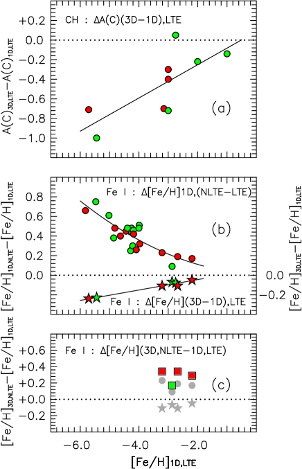
Figure 2: 3D and NLTE corrections as a function of [Fe/H]_1D,LTE. In all panels, red and green symbols represent dwarfs and giants, respectively, from the work of Amarsi et al. (2016), Collet et al. (2006, 2007, 2018), Ezzeddine et al. (2017), Frebel et al. (2008), Gallagher et al. (2016) and Spite et al. (2013) (see Table 2). The panel (a) ordinate shows $\Delta$$A$(C)_(3D-1D),LTE, while (b) presents $\Delta$[Fe/H]_{1D,(NLTE-LTE)} and $\Delta$[Fe/H]_(3D-1D),LTE. (The lines represent the least-squares best fits: (a) $\Delta$$A$(C)_(3D-1D),LTE = $A$(C)_3D,LTE – $A$(C)_1D,LTE = 0.087 + 0.170 [Fe/H]_1D,LTE, and (b) $\Delta$[Fe/H]_{1D,(NLTE-LTE)} = [Fe/H]_1D,NLTE – [Fe/H]_1D,LTE = 0.013 – 0.011 [Fe/H]_1D,LTE + 0.019 [Fe/H]_1D,LTE² and $\Delta$[Fe/H]_(3D-1D),LTE = [Fe/H]_3D,LTE – [Fe/H]_1D,LTE = 0.061 + 0.053 [Fe/H]_1D,LTE). In panel (c) the grey symbols repeat the Amarsi et al. (2016) [Fe/H] (3D–1D),LTE and 1D,(NLTE-LTE) corrections from panel (b), while the squares stand for $\Delta$[Fe/H] = [Fe/H]_3D,NLTE – [Fe/H]_1D,LTE. We adopt [Fe/H]_3D,NLTE – [Fe/H]_1D,NLTE = 0.12. See text for discussion.

There are nine cases for which CH corrections are available, from the work of Collet et al. (2006, 2007, 2018), Frebel et al. (2008), Spite et al. (2013), and Gallagher et al. (2016). Six of the nine cases are based on analysis of stars, while three are determined entirely from model atmosphere comparisons. The data are also plotted in Figure 2, where the upper panel (a) presents $\Delta$$A$(C)_(3D-1D),LTE = $A$(C)_3D,LTE – $A$(C)_1D,LTE versus [Fe/H]_1D,LTE. Red and green symbols refer to dwarfs and giants (defined here to have $\log g$ larger or smaller than 3.35), respectively. The full line in the figure represents the linear least-squares best fit to the data, which is given by: $\Delta$$A$(C)_(3D-1D),LTE = 0.087 + 0.170 [Fe/H] (9 points, with RMS = 0.24).

Further literature data are available that provide 1D,LTE corrections of Fe I. Results from the work of Amarsi et al. (2016), Collet et al. (2006, 2007, 2018), Ezzeddine et al. (2017), and Frebel et al. (2008) are presented in Columns (4) – (7) of Table 2, where there are 22 stars, all having 1D,NLTE-LTE corrections; seven have 3D,LTE information; and four have 3D,NLTE data.

The 3D–1D,LTE and 1D,NLTE-LTE corrections for Fe are plotted in Figure 2, panel (b) as a function of [Fe/H]_1D,LTE. The panel also presents linear and quadratic least-squares lines of best fit, the equations for which are: $\Delta$[Fe/H]_{1D,(NLTE-LTE)} = [Fe/H]_1D,NLTE – [Fe/H]_1D,LTE = 0.013 – 0.011 [Fe/H]_1D,LTE + 0.019 [Fe/H]_1D,LTE² (22 points, with RMS = 0.09) and $\Delta$[Fe/H]_(3D-1D),LTE = [Fe/H]_3D,LTE – [Fe/H]_1D,LTE = 0.061 + 0.053 [Fe/H]_1D,LTE (7 points, with RMS = 0.02).

We conclude this section with two comments. First, as the reader can confirm from inspection of the middle panel (b) of Figure 2, the (3D–1D),LTE corrections are in the opposite sense to those for the 1D,(NLTE-LTE) case. Second, inspection of panels (a) and (b) of Figure 2 reveals that there appears to be no significant difference between the distributions of the dwarf and giant stars. In what follows, we shall assume that this is the case.

3.2 [Fe/H] 3D,NLTE Corrections

The previous section presents [Fe/H]_3D,LTE and [Fe/H]_1D,NLTE corrections (relative to [Fe/H]_1D,LTE) abundances. What we would really like, however, are [Fe/H]_3D,NLTE corrections. The very limited available data in Table 2 are from Amarsi et al. (2016) and are shown in the bottom panel (c) of Figure 2. The grey symbols are the [Fe/H] (3D–1D),LTE and 1D,(NLTE-LTE) corrections from the middle panel of the figure, while the square symbols above them are the [Fe/H]_3D,NLTE – [Fe/H]_1D,LTE corrections. A very significant result of the bottom panel (c) is that while the [Fe/H]_1D,NLTE – [Fe/H]_1D,LTE corrections in (b) are positive and the [Fe/H]_3D,LTE – [Fe/H]_1D,LTE values, also in (b), are negative, the [Fe/H]_3D,NLTE – [Fe/H]_1D,LTE corrections in (c) are positive and larger than [Fe/H]_1D,NLTE – [Fe/H]_1D,LTE (from (b)), by 0.08 – 0.15 dex (with a mean value 0.12). This suggests that when 3D and NLTE effects are treated in a self-consistent manner the NLTE corrections dominate. In the absence of other information, in the following we shall assume that [Fe/H]_3D,NLTE – [Fe/H]_1D,NLTE = 0.12.

3.3 High-excitation C I lines and 3D,NLTE corrections for CH

As emphasized above, 3D,NLTE carbon abundances based on the analysis of the G-band are currently unavailable due to the intractability of the CH molecule to NLTE analysis. The near-infrared, high-excitation C I lines, however, are not affected by this problem. With excitation potentials $\sim$ 7 eV, these lines form deep in the stellar atmosphere, well below the outer layers where the 3D effects are significant. We now use literature C I abundance analyses to obtain estimates of 3D,NLTE corrections for CH-based values. By comparing the results for stars for which carbon abundances have been obtained from analyses of both the CH G-band and near-infrared C I lines, we then estimate the sense and size of the 3D,NLTE corrections for the CH-based carbon abundances discussed in the previous section.

3.3.1 Carbon abundances from the near-infrared C I lines

Fabbian et al. (2009) present $A$(C)_1D,NLTE abundances for 43 metal-poor dwarfs and subgiants in the abundance range –3.2 $<$ [Fe/H] $<$ –1.3, based on analysis of the high-excitation C I 9094.8 and 9111.8 Å lines (EP = 7.49 eV). They also provide atmospheric parameters $T_{\rm eff}$, $\log g$, and [Fe/H]_1D,LTE, together with [C/H]_1D,LTE, and [C/H]_1D,NLTE for two values of the Drawin scaling factor S_H (= 0.0 and 1.0). In what follows we shall adopt the average of these two values of [C/H] _1D,NLTE. Fabbian et al. (2009) also noted that the high-excitation potential of the C I lines would very likely lead to only small (3D–1D),NLTE corrections, given that these lines are formed sufficiently deep in the atmospheres of the stars to be insensitive to the 3D effects, which are significant principally in the outermost layers. This expectation is supported by the work of Dobrovolskas et al. (2013) from their comprehensive analysis of (3D–1D),LTE corrections for a large number of atomic species as a function of excitation potential, among other parameters. In particular their Figure 4 shows that for neutral carbon lines having EP = 6eV, $\Delta$(3D–1D),LTE = 0.04 dex. That is, effectively, $A$(CI)_1D,NLTE = $A$(CI)_3D,NLTE. (For convenience, in this sub-section we shall refer to abundances based on C I lines as $A$(CI) and those on the CH features as $A$(CH).)

To proceed further we also require CH-based carbon abundances for these stars. For 23 of the Fabbian et al. sample we obtained high-resolution, high signal-to-noise spectra from astronomical archives. Details of this sub-sample are presented in Table 3. Columns (1) – (4) contain the star name, $T_{\rm eff}$, $\log g$, and [Fe/H] from Fabbian et al. (2009), while columns (5) – (6) present their values of $A$(CI)_1D,LTE and $A$(CI)_1D,NLTE. Columns (10) – (11) of the table contain the $S/N$ of the spectra and the archives from which the CH data were obtained.

To obtain $A$(CH) we proceeded as follows. For each star we co-added multiple spectra as available, followed by continuum normalization. Using the atmospheric parameters of Fabbian et al. (2009), model-atmospheric spectra of each star were computed for several carbon abundances over the range 4305 – 4330 Å. We refer the reader to Yong et al. (2013a) for details of the technique. In brief, we used the code MOOG (Sneden, 1973), as modified by Sobeck et al. (2011), together with the model atmospheres of Castelli & Kurucz (2003). In the linelist, the data for CH lines were provided by B. Plez et al. (2009, private communication; see Masseron et al., 2014). Other pertinent data are: we adopted microturbulence = 1.5 km s^-1 and [O/Fe] = 0.40, and note that the results are insensitive to the latter, given the relatively high effective temperatures of these dwarfs. The resulting abundances are presented in Table 3, where columns (7) – (9) contain $A$(CH)_1D,LTE, $A$(CH)_3D,LTE, and $A$(CH)_3D,LTE – $A$(CH)_1D,LTE, respectively ($A$(CH)_3D,LTE was computed using the (3D–1D),LTE corrections presented in Section 3.1 above). For comparison purposes, we also present in Table 3 the CH based literature abundances for CD $-24^{\circ}\,17504$ from Jacobson & Frebel (2015), and G64-12 and G64-37 from Placco et al. (2016a). We note that the mean difference between our results and those of Jacobson & Frebel (2015) and Placco et al. (2016a) is $\langle$$\Delta$$A$(CH)_1D,LTE$\rangle$ = 0.06.

3.3.2 Estimating the 3D,NLTE corrections appropriate for the CH G-band

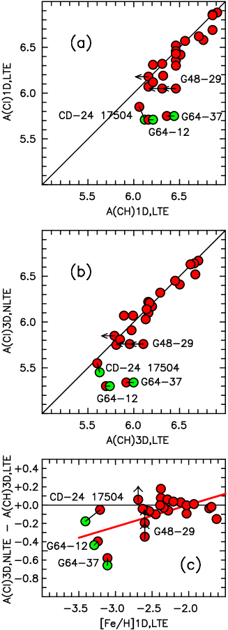
Figure 3: The comparison between the 3D and 1D carbon abundances determined from analysis of the CH G-band and C I high-excitation lines: (a) $A$(CI)_1D,NLTE vs $A$(CH)_1D,LTE, (b) $A$(CI)_3D,LTE vs. $A$(CH)_3D,LTE, and (c) $\Delta$$A$(C) = $A$(CI)_3D,NLTE – $A$(CH)_3D,LTE as a function of [Fe/H]_1D,LTE. The red and green symbols represent stars for which CH-based abundances come from the present work and the literature, respectively. In (a) and (b) the full line represents the 1-1 relation, while in (c) the wide red line is the linear least-squares best fit to the data. See text for discussion.

We now estimate the sense and size of 3D,NLTE corrections appropriate for the CH G-band analysis. In Figure 3 the top two panels (a and b) present $A$(CI)_1D,LTE vs. $A$(CH)_1D,LTE and $A$(CI)_3D,LTE vs. $A$(CH)_3D,LTE, respectively, for heuristic purposes, to give the reader a feeling for the changes brought about by 3D and NLTE effects. The bottom panel (c) of the figure shows $\Delta$$A$(C) = $A$(CI)_3D,NLTE – $A$(CH)_3D,LTE as a function of [Fe/H]_1D,LTE. If the C I and CH estimates of carbon abundances accurately and self-consistently include all 3D and NLTE effects, $\Delta$$A$(C) should be zero. Given (as discussed above) that $A$(CI)_1D,NLTE = $A$(CI)_3D,NLTE, any departure of $\Delta$$A$(C) from zero represents an estimate of the CH 3D,NLTE corrections needed for these stars. The negative values of $\Delta$$A$(C) for G64-12 and G64-37 in Figure 3 indicate that their $A$(CH)_3D,LTE values are larger than $A$(CH)_3D,NLTE. That is, a further negative correction is required to produce more accurate $A$(CH)_3D,NLTE values. The full red line in Figure 3 is the linear least-squares fit to the data (excluding stars BD $-13^{\circ}\,3442$ and G 48-29, for which only limits are available) which is given by $A$(CI)_3D,NLTE – $A$(CH)_3D,LTE = 0.483 + 0.240 [Fe/H]_1D,LTE (24 points, with RMS = 0.17) and which we take as the in-principal improvement necessary to $A$(CH)_3D,LTE to correct it to $A$(CH)_3D,NLTE.

That said, given the weakness of the CH features and C I lines in metal-poor dwarfs with [Fe/H] $<$ –3.0 (see Jacobson & Frebel, 2015, Placco et al., 2016a, and Fabbian et al., 2009), in what follows we shall assume that this correction is not well-determined below [Fe/H] $\;\buildrel<\over{\sim}\;$ –3.0, and make the conservative assumption that $A$(CI)_3D,NLTE – $A$(CH)_3D,LTE = 0.0, for all [Fe/H], and hence $A$(CH)_3D,NLTE = $A$(CH)_3D,LTE. The reader should bear in mind that the 3D,NLTE corrections we shall present in what follows are most likely less extreme than would be obtained by adoption of the equation in the previous paragraph.

4 Revised $A$(C) vs. [Fe/H] and [C/Fe] vs. [Fe/H] Diagrams

4.1 The Yoon et al. (2016) sample of CEMP stars

With the 3D–1D and NLTE–LTE corrections in hand, we now investigate their effect on the distribution of the CEMP-no stars in the ($A$(C), [Fe/H]) and ([C/Fe], [Fe/H]) $-$ planes. Figure 4 presents the data for the CEMP-no and CEMP-s objects compiled by Yoon et al. (2016), together with those for an additional recently reported eight CEMP-no stars presented in Table 4, and four stars identified in Table 6. The effects of the corrections to $A$(C), [C/Fe], and [Fe/H] are presented in the three rows of the figure. The uppermost row, panels (a) and (b), show data obtained using 1D,LTE for $A$(C)_1D,LTE and [C/Fe]_1D,LTE vs. [Fe/H]_1D,LTE, respectively. Also shown in the top left panel (a) are the the ellipses containing the Groups I, II, and III of Yoon et al. (2016), together with the “high-carbon band” (horizontal orange line) and the “low-carbon band” (horizontal light blue line) of Spite et al. (2013), Bonifacio et al. (2015, 2018), and Caffau et al. (2018) (truncated on the right by the [C/Fe] = +1.0 locus). In these panels, (a) and (b), red and grey symbols refer to CEMP-no stars on the one hand, and CEMP-s stars on the other, and in what follows in the middle and bottom rows the symbol for each star will retain the same color as adopted in these uppermost panels. The full and dotted lines in all panels represent the loci of the [C/Fe] $>$ +0.7 divide between C-normal and CEMP stars, and [C/Fe] = 0.0, respectively.

In the middle row, panels (c) and (d), we show the effect of (3D–1D),LTE corrections. In the left panel (c), the $A$(C) distribution lies well below that of the 1D,LTE data, and at lower [Fe/H], than in panel (a). Here the abscissa becomes [Fe/H]_3D,LTE in both panels, while the ordinate is $A$(C)_3D,LTE on the left and becomes [C/Fe]_3D,LTE = [C/H]_3D,LTE $-$ [Fe/H]_3D,LTE on the right. In both panels one sees that the distribution moves to lower values of [Fe/H], while the carbon abundances also decrease. With these corrections, a significant number of stars now fall below the CEMP limit of [C/Fe] $>$ +0.7: the number of CEMP-no stars has reduced from 130 in the top row to 68 in the middle row, a decrease of 48%.

The bottom row of Figure 4, panels (e) and (f), presents the changes when 3D,NLTE corrections are applied to the 1D,LTE data in the top row. To produce [Fe/H]_3D,NLTE we use the 3D,NLTE corrections of Section 3.2, and for $A$(C)_3D,NLTE and [C/Fe]_3D,NLTE adopt corrections following the discussion in Section 3.3. In the context of carbon 3D,NLTE effects, we recall that in Section 3.3 a comparison of carbon abundances derived from the CH G band and from high-excitation C I lines leads to the conclusion that the (currently unknowable) NLTE effects on the G band appear not to increase CH based abundances (and indeed hint that they will further decrease them; see Figure 3). Given the the extreme weakness of the CH and C I features and the sparseness of data for stars with [Fe/H] $<$ –3.0, we choose to assume $A$(C)_3D,NLTE = $A$(C)_3D,LTE for the purposes of the present discussion.

Inspection of the bottom panels (e) and (f) of Figure 4 shows that 3D,NLTE considerations have an enormous effect on the number of putative C-rich stars (exclusively on those in the Yoon Group II, which have lower $A$(C)_1D,LTE). The number of CEMP-no stars having [C/Fe] $>$ +0.7 and [Fe/H] $<$ –2.0 in the upper left panel (a) has decreased from 130 to 35 in the bottom left panel (e) $-$ a reduction of 73%. Against this background it is worth noting that it is the number of CEMP-no, Group II stars that has decreased; the number of CEMP-no, Group III stars, which are considerably more carbon rich, is not affected.

Said differently, 3D,NLTE effects constitute the perfect storm for those who might wish to understand the carbon abundances of metal-poor stars by adopting results based on the 1D,LTE assumptions. First, 1D,LTE overestimates CH-based carbon abundances and, second, it underestimates iron abundances (determined from Fe I lines) relative to those determined using 3D,NLTE. Both effects inflate [C/Fe], and in both the [C/Fe] vs. [Fe/H], and the $A$(C) vs. [Fe/H] planes the effects of the transformations are huge. A third effect is that in these planes the C-rich stars are seen against a considerably larger C-normal population, in which errors of measurement in both estimates of, say, 0.2 $-$0.3 dex have the potential to move C-normal stars into the sparse [C/Fe]-rich region (i.e., into that of the Group II stars).

It has been suggested to the authors that the above results may be affected by the strong $\log g$ sensitivity of the Placco [C/Fe] corrections present in the Yoon et al. (2016) data compilation. That is, while the corrections are negligible for main sequence stars, they are large ($\sim$+0.5 dex for objects towards the top of the giant branch). Examination of the Placco corrections for [Fe/H] = –3.0 (a representative value for the present discussion) against the [Fe/H] = –3.0, age = 12 Gyr isochrone of Demarque et al. (2004) shows that only above $\log g$ = 2.0 do they become larger than $\sim$0.05. When we then replot our Figure 4 including only stars having log g $<$ 2.0, we find that the areas covered by the stars are not significantly changed from the point of view of the present discussion of the 3D and NLTE predictions. In particular, the number of CEMP-no stars on the 1D,LTE panel is 66, which reduces to 40 for 3D,LTE, and 24 for 3D,NLTE – reductions of 39 and 64%, respectively (compared with 48% and 73% for the complete sample).

4.2 The Yong et al. (2013a) sample of CEMP and C-normal stars

We have also applied the above formalism to the literature sample of 190 extremely metal-poor stars of Yong et al. (2013a). An advantage of this sample is that it is not limited to only CEMP stars as is that of Yoon et al. (2016). It was used by Yong et al. (2013b) to place constraints on the MDF of metal-poor stars, and on the fraction of C-rich stars as a function of metallicity ([Fe/H]). Re-examination of the Yong et al. (2013a) sample has the potential to highlight the effects that the correction of abundances from 1D,LTE to 3D,LTE and 3D,NLTE has on these important relationships, not only on the C-rich stars but also on those that are C-normal.

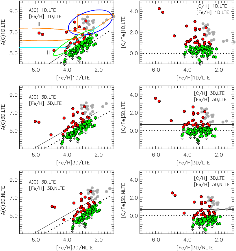
Figure 5: Carbon vs. iron abundances for the data sample of Yong et al. (2013a), where the format is the same as that of Figure 4, with the exception that the green symbols represent 1D,LTE C-normal stars. The color for each individual star is as determined in the 1D,LTE uppermost panels. The thin full and dotted lines refer to the [C/Fe] = +0.7 and 0.0 loci. See text for discussion.

Figure 5 presents $A$(C) and [C/Fe] as a function of [Fe/H], where the layout in the figure is the same as that of Figure 4 and we have adopted the same 3D,LTE and 3D,NLTE corrections. The red symbols refer to CEMP-no stars that have carbon abundances based on detections yielding [C/Fe]_1D,LTE $>$ +0.7 and [Ba/Fe]_1D,LTE $<$ 0.0; the green symbols represent C-normal stars with either carbon detections or limits having [C/Fe]_1D,LTE $<$ +0.7; and grey circles stand for CEMP-s stars. As in our discussion of Figure 4, in the middle and bottom rows the symbol for each star retains the same color as adopted in the upper, 1D,LTE, panels. For 1D,LTE-based abundances and [Fe/H]_1D,LTE $<$ $-$2.0, there are some 88 C-normal and 28 CEMP-no stars. CEMP-no stars represent a fraction of 24% of the total of CEMP-no plus C-normal stars.

Figure 5 also permits an estimate of the 3D and NLTE effects on the fraction of CEMP-no stars in a sample containing both C-normal and CEMP-no stars. As in Figure 4, the middle and bottom rows refer to abundances determined assuming 3D,LTE and 3D,NLTE, respectively, and here too large fractions of 1D,LTE CEMP-no stars become C-normal when investigated in 3D and NLTE. For stars with [Fe/H]_3D,LTE $<$ $-$2.0 in the bottom row, $A$(C)_3D,NLTE vs. [Fe/H]_3D,NLTE, there are some 108 C-normal and 9 CEMP-no stars, leading to a fraction of CEMP-no stars of 8%, a very significant decrease compared with the 1D,LTE fraction of 24%. (As noted in the previous section, it is the number of Group II stars that is decreasing, while that of their Group III counterparts remains unchanged.)

A somewhat surprising result evident in the bottom panels is the number of stars well below [C/Fe]_3D,NLTE $\;\buildrel<\over{\sim}\;$ 0.0. For these stars, and ignoring those having only carbon abundance limits, $\langle$[C/Fe]_3D,NLTE$\rangle$ = –0.42 $\pm$ 0.03, with dispersion $\sigma$ = 0.27 (82 objects). In comparison, for dwarfs with –3.2 $<$ [Fe/H] $<$ –2.0, Amarsi et al. (2019, see their Figure 1), from analysis of the infrared high-excitation C I lines, report [C/Fe]_3D,NLTE values $\sim$ +0.1 dex. While a full explanation of the present G-band abundances lies outside the scope of the present work, we make two comments. The first is that the effect appears to be gravity dependent, insofar as for giants ($\log g$ $<$ 3.35) in the present sample we find $\langle$[C/Fe]_3D,NLTE$\rangle$ = –0.49 $\pm$ 0.04 (61 stars) and for dwarfs ($\log g$ $>$ 3.35) $\langle$[C/Fe]_3D,NLTE$\rangle$ = –0.24 $\pm$ 0.03 (21 stars). Further support for the higher value obtained for dwarfs is provided by the data for those in our Table 3. For the stars in the table with CH-based carbon abundances determined in the present work, and excluding stars with only limits, we find $\langle$[C/Fe]_3D,NLTE$\rangle$ = –0.18 $\pm$ 0.03. A possible explanation of the effect is that the giant abundances have been underestimated. The second point is that Gallagher et al. (2016) have reported that the $A$(C) 3D,LTE corrections are a function of $A$(C) (see our Section 6).

4.3 A comment on the CEMP-no status of CD $-24^{\circ}\,17504$, G64-12, and G64-37

CD $-24^{\circ}\,17504$, G 64-12, and G 64-37 were recently re-classified as CEMP-no stars by Jacobson & Frebel (2015) and Placco et al. (2016a). They are all extremely metal-poor near main-sequence-turnoff stars with similar $T_{\rm eff}$, $\log g$, [Fe/H]_1D,LTE (–3.41, –3.29, –3.11), and [C/Fe]_1D,LTE (1.10, 1.07, and 1.12), together with [Ba/Fe] = $<$–1.05. –0.36, and –0.06, respectively. The 3D,LTE and 3D,NLTE iron and carbon abundances of these objects, however, argue that all of them are C-normal, with an average carbon abundance of $\langle$[C/Fe]_3D,LTE$\rangle$ = 0.74 and $\langle$[C/Fe]_3D,NLTE$\rangle$ = 0.26. Some support for this conclusion is suggested by the fact that their discovery as metal-poor stars is based on their halo kinematics (Carney & Peterson, 1981 and Ryan et al., 1991), without knowledge concerning their abundance characteristics, i.e., they are an unbiased sample with respect to abundance. If one accepts that the CEMP fraction at [Fe/H] = –3.2 is $\sim$ 0.30, based on 1D,LTE analyses (Yong et al., 2013b, Lee et al., 2013), the probability that all three of them should be CEMP stars is only $\sim$ 3%.

4.4 On the Nature of the Group I CEMP-no Stars

One of the most intriguing aspects of the Yoon et al. (2016) $A$(C) vs. [Fe/H] diagram is that while all of the CEMP-s stars belong to Group I and their Groups II and III contain only CEMP-no stars, there is a non-negligible fraction of CEMP-no stars within the Group I boundary. Inspection of our Figure 4 shows there are 19 such CEMP-no Group I stars,which represent 14% of the group. The obvious question is: why is the abundance of carbon relative to hydrogen higher by some $\sim$1 dex in the CEMP-no, Group I stars compared with that of the majority of their counterparts in Groups II and III? For future reference, Table 5 presents details of the 19 CEMP-no, Group I stars.

To our knowledge, the significance of this subset of CEMP-no stars was first appreciated by Hansen et al. (2016b), who reported that five of their sample of 24 CEMP-no stars (HE 0219–1739, HE 1133–0555, HE 1410+0213, HE 1150–0428, and CS 22957–027) lie in or close to the “high-carbon band” first reported by Spite et al. (2013) (in large part their “high-carbon band” is related to the Yoon et al. (2016) Group I). Hansen et al. (2016b) noted that three of these are binaries. They commented: “Should the majority [of this subset of CEMP-no stars] turn out to be members of binary systems … and in particular if there are signs that mass transfer has occurred, this would lend support to the existence of AGB stars that produce little if any s-process elements”. Arentsen et al. (2018) have further addressed the issue and reported that this CEMP-no subset has a “binary fraction … of $47^{\,+15\,}_{\,-14}\%$ for stars with higher absolute carbon abundance”. Inspection of our Table 5 shows that four out of nine CEMP-no, Group I (i.e., $\sim$ 45%) stars for which data are available are binary.

A further related conjecture is that the putative AGB stars of Hansen et al. may have been the 7 M_⊙, initial rotational velocity 800 km s^-1 spinstars of Meynet et al. (2006), which very nicely reproduce the light-element abundance patterns of the CEMP-no stars. Taking the potential binary-with-mass-transfer hypothesis further, if one assumes that the number of Group I CEMP-s stars is proportional to the number of putative polluting stars in the mass range (say) 2 – 6 M_⊙ (cf., Lugaro et al., 2012), while the number of Group I CEMP-no is proportional to that of those in the mass range (say) 6 – 8 M_⊙, (e.g., Meynet et al., 2006), and further assumes that star formation followed the Salpeter Initial Mass Function, one finds that the ratio of AGB stars in the 6 – 8 M_⊙ range to those in the two mass ranges together is 0.09, similar to the observed fraction, 0.14, noted above, which CEMP-no, Group I stars contribute to the total Group I sample.

5 The Metallicity Distribution Function (MDF) and the CEMP-no Fraction

The MDF of the Galaxy’s very metal-poor stars (VMP, [Fe/H] $<$ $-$2.0) is complicated by the fact that the sample is inhomogeneous, comprising several sub-populations. A topic closely related to the MDF is the size of the CEMP-no fraction, and its dependence on metal abundance. Any understanding of these will ultimately turn on a closer knowledge of the metallicity distribution functions of the halo’s several components. In this context, the two major C-rich groups, of CEMP-s and CEMP-no stars, provide an interesting challenge. We refer the reader to Papers III and IV of this series (Yong et al., 2013b, Norris et al., 2013), and references therein, for an effort to better understand the role of these sub-populations. Other important investigations include those of Carollo et al. (2012, 2014) and Lee et al. (2013, 2017). The question we shall address here is the role that 3D,NLTE corrections to 1D,LTE carbon and iron abundances play in our understanding of these matters.

5.1 MDFs

We use the formalism of Yong et al. (2013b) to examine the MDF of the Yong et al. (2013a) sample discussed in the previous section. C-rich stars ([C/Fe] $>$ +0.7) were included only if an abundance was available in Yong et al. (2013a) (i.e., those with an abundance limit were excluded), while both detections and limits were included in the C-normal regime ([C/Fe] $<$ +0.7). In the left panel of Figure 6, the logarithm (base 10) of the generalized histogram (adopting a Gaussian kernel having $\sigma$ = 0.30 dex) is presented as a function of [Fe/H], where [Fe/H] is adopted as proxy for the total heavy element abundance. As in our earlier work, we investigate the MDF for stars with [Fe/H] $<$ $-$3.0, and to which we have applied sample completeness corrections. In the figure, the green-shaded areas pertain to the combination of the CEMP-no and CEMP-s subgroups, the grey-shaded areas refer to C-normal stars, and the small unshaded (upper) areas stand for stars for which the carbon abundance was not measured.

The top panel of the figure is based on 1D,LTE abundances, while the middle and bottom panels present 3D,LTE and 3D,NLTE results, respectively. The outstanding feature of the MDFs is the decreasing role of the C-rich stars ([C/Fe] $>$ +0.7) when 3D and non-LTE corrections are applied, as would be expected from inspection of Figure 5.

5.2 CEMP-no fraction

In the right panel of Figure 6 we present the manner in which the fraction of CEMP-no stars increases as [Fe/H] decreases when one changes from 1D,LTE to 3D,LTE, to 3D,NLTE. Here we define the CEMP-no fraction as N_CEMP-no/(N_C-normal + N_CEMP-no + N_CEMP-s), where we include the CEMP-s stars in the equation on the assumption they were once C-normal stars, in order to obtain a more complete fraction. In practice, this has only a small effect in the present discussion, given there are relatively few CEMP-s stars with [Fe/H] $<$ $-$3.0.

In this panel, the full lines represent the fraction of CEMP-no stars, while for comparison purposes the dashed line in each of the lower two subpanels is the 1D,LTE fraction presented in the topmost subpanel. In the top, middle, and bottom panels the fraction of CEMP-no stars with –4.5 $<$ Fe/H] $<$ –3.0 are 0.30, 0.15, and 0.12, respectively. We also note that while in this figure all stars with [Fe/H] $<$ –4.5 are C-rich, the relatively complete sample upon which this is based contains only three such objects. We recall from our Tables 1 and 6 that, at time of writing, some 14 stars are now known with [Fe/H] $<$ –4.5, a large majority of which is C-rich (see Frebel & Norris, 2015, Frebel et al., 2015, Caffau et al., 2016, Aguado et al., 2018a, Aguado et al., 2018b, and Starkenburg et al., 2018). In the present context, perhaps the most significant result one might take from the panel is that when one includes 3D and NLTE corrections a separation between the population of C-rich stars with [Fe/H] $<$ –4.5, and that with [Fe/H] $>$ –4.5 becomes clearer, and more significant.

6 Uncertainties

We alert the reader to some uncertainties implicit in the present work.

6.1 The CH 3D,LTE corrections are a function of $A$(C)

Gallagher et al. (2016) report that G band 3D,LTE corrections are a function not only of [Fe/H], but also of $A$(C), and present a comprehensive investigation of 3D corrections for CEMP dwarfs on the ranges $-$3.0 $<$ [Fe/H] $<$ $-$1.0, 5900K $<$ $T_{\rm eff}$ $<$ 6500K, 4.0 $<$ $\log g$ $<$ 4.5, 6.0 $<$ $A$(C)_3D $<$ 8.5, and for two values of C/O = 0.21 and 3.98. They emphasize that the corrections are sensitive to the C/O ratio, and adopt the value of C/O = 0.21 as most appropriate for the CEMP-no stars. We note here that for CEMP-no stars the available abundance data suggest that [O/Fe] increases linearly with [C/Fe] (e.g., Norris et al., 2013, Figure 2), and therefore a constant value of C/O.

6.2 How trustworthy is the Drawin scaling factor S_H treatment of the neutral hydrogen?

In Section 3.3, the carbon abundances based on the analysis of high-excitation C I lines adopted the formalism of Drawin to describe the influence of inelastic hydrogen atom collisions. Barklem et al. (2011), however, report that “Quantitatively, the Drawin formula compares poorly with the results of the available quantum mechanical calculations, usually significantly overestimating the collision rates by amounts that vary markedly between transitions.” That said, we recall here, from Section 3.3, the excellent agreement between the analyses of Fabbian et al. (2009) and Amarsi et al. (2019), the latter of which adopts “modern descriptions of the inelastic collisions with neutral hydrogen”.

6.3 Are differences between photometric and spectroscopic $T_{\rm eff}$ values a problem?

An evergreen uncertainly in the determination of chemical abundances based on 1D,LTE analyses is the differences that result when $T_{\rm eff}$ values are based on different assumptions. Suffice it here to say that [Fe I/H]_1D,LTE values can differ systematically by values of order 0.3 – 0.4 dex between analyses that adopt photometric $T_{\rm eff}$ values and those that use spectroscopically determined ones (see e.g., Roederer et al., 2014, Table 17). This could be important in determining Group II, CEMP-no status, for example, in Figures 4 and 5.

7 The Abundances of Other Elements in the CEMP-no Stars

7.1 The Light Elements Na, Mg, and Al

A distinctive feature of the CEMP-no stars is that they also exhihit overabundances of Na, Mg, and Al, to varying degrees in size and from element to element, while only small (if any) differences are found in the relative abundances, [X/Fe], on the range Si through to the heavy-neutron-capture elements (see Frebel & Norris, 2015, and references therein). Indeed, the interpretation of [X/Fe] as a function of atomic number is a key to an understanding of the origin of these stars (see Umeda & Nomoto, 2003, Meynet et al., 2006, Heger & Woosley, 2010, Nomoto et al., 2013, Takahashi et al., 2014, Maeder & Meynet, 2015, and references therein). That said, insofar as discussed in Section 4, many stars which under the 1D,LTE assumption were designated CEMP-no become C-normal when interpreted using 3D,NLTE, it is probably fair to say that we may not yet have a complete understanding of these abundance patterns. A potential example of this problem is the report by Yoon et al. (2016) that their Group II and Group III CEMP-no stars have different Na and Mg distributions. A second interesting phenomenon, described in Section 4.4, is the existence of a $\sim$15% subpopulation of CEMP-no stars in their Group I, which principally comprises only CEMP-s stars. What is the light element signature of these stars?

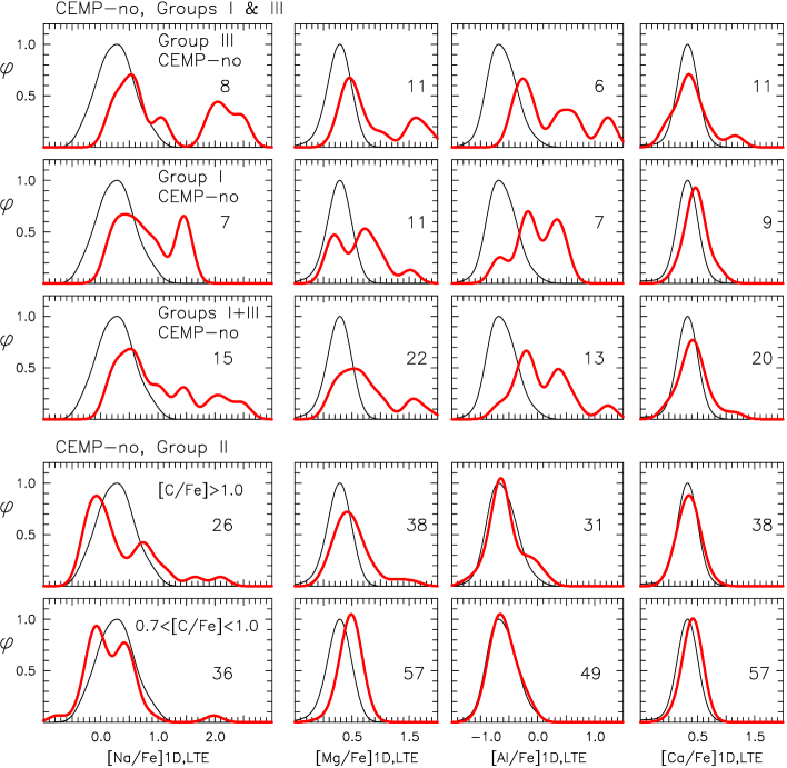
Figure 7: Generalized histograms for (1D,LTE) [Na/Fe], [Mg/Fe], [Al/Fe], and [Ca/Fe] abundances (with Gaussian kernels of 0.30 dex). The red thicker lines are for the CEMP-no stars of Yoon et al. (2016) and Table 4 of the present work, while the thinner black lines represent the C-normal stars of Yong et al. (2013a). The legends contain the Group memberships of the samples, where the details in the leftmost panels apply to all of the panels in that row. In the legends in the bottom two rows, [C/Fe] is the 1D,LTE value. The number in each panel indicates the number of stars included in the histogram.

Figure 7 shows generalized histograms of 1D,LTE abundances for [Na/Fe], [Mg/Fe], and [Al/Fe], together with [Ca/Fe] (which exhibits small if any variation, and is shown here only for comparison purposes). In each sub-panel the thicker red line pertains to CEMP-no stars, and the thinner black one to C-normal objects; and the areas under both curves have been normalized to be the same. In the top three rows of the figure, results are presented for the Group I and III CEMP-no stars, where from top towards bottom we consider Group III, Group I, and Group III + Group I CEMP-no stars, respectively. (For the C-normal stars the same histogram is presented in all sub-panels of the same element.) The numbers of CEMP-no stars involved are presented in each sub-panel, and while they are small, one’s first impression is that the Na, Mg, and Al distributions are similar in both Groups I and III, at least insofar as significant overabundances are evident in all panels; and while more data are required, the figure suggests that Group I and Group III CEMP-no stars have experienced similar enrichment pathways.

The bottom two rows present abundances for CEMP-no, Group II stars. The upper of the two rows is for [C/Fe]_1D,LTE $>$ +1.0, while the lower is the result for +0.7 $<$ [C/Fe]_1D,LTE $<$ +1.0. Inspection of the two panels suggests a broader distribution of each of Na, Mg, and Al abundances (but not of Ca) in the upper row than in the lower one. The simplest interpretation of this difference is that the majority of the stars in the range +0.7 $<$ [C/Fe]_1D,LTE $<$ +1.0 does not have overabundances of Na, Mg, and Al, or that their carbon abundances have been overestimated. This could also explain, at lease in part, the report by Yoon et al. (2016) that the Group II and III CEMP-no stars have experienced different Na and Mg enrichment pathways.

It has been suggested to us that the Yoon et al. (2016) Group II stars are not CEMP-no stars, and have apparently large carbon abundances due to errors of measurement, and/or of the Placco et al. (2014) corrections. This is not obvious to us, given that the Group II stars with [C/Fe] $>$ +1.0 are identified as CEMP-no by both Yoon et al. (2016) and Caffau et al. (2018) (see Figure 4), and that some of them have Na, Mg, and Al overabundances. Further work is needed to address this issue. The outstanding question for us is: why is the distribution of CEMP-no stars in Figure 4 so obviously non-uniform, leading Yoon et al. (2016) to identify two groups. We shall return to this in Section 8.

We conclude our discussion by noting the enigmatic result that while overabundances of Na and Mg in the CEMP-no stars are clear in all panels which present these elements in Figure 7 (except for Mg in the bottom row), the histograms also appear to have a component that has close to the solar abundance ratio. More data are clearly required to confirm and address the reality and implications of this effect.

7.2 [Sr/Ba] and the nature of the CEMP-no, Group I stars

How may one understand the CEMP-no, Group I stars. In Section 4.4 we noted the suggestion of Hansen et al. (2016b), supported by further work of Arentsen et al. (2018), that the binarity of a significant fraction of these stars might signal mass transfer in a system in which the AGB star did not experience s-process enhancement. We also pointed out that the ratio of Group I CEMP-no to CEMP-s stars is consistent with higher masses for the putative AGB star enrichment of the CEMP-no, Group I stars than exists for their CEMP-s, Group I counterparts.

The question then is, do descriptions of massive AGB stars that produce primary carbon, but little or no s-process enhanced material, exist in the literature? The obvious answer is the extremely metal-poor spinstars of Meynet et al. (2006) and Frischknecht et al. (2010, 2012), which do not produce the s-process pattern, but rather overproduce Sr relative to Ba. In this context, Hansen et al. (2019) have proposed [Sr/Ba] as a parameter to distinguish between the various CEMP subclasses, based in part on the result of Frischknecht et al. that Sr is overproduced more relative to Ba than is observed in the CEMP-no and C-normal stars.

Against this background, Figure 8 presents [Sr/Ba]_1D,LTE as a function of [Fe/H]_1D,LTE for CEMP-no stars of Group I (red star symbols) and III (red circles), together with CEMP-s stars (grey circles), based on data from the literature. The important result here is that, taken as a whole, the [Sr/Ba] values of the CEMP-no, Group I objects are larger than those of the CEMP-s stars. We also note that most of the [Sr/Ba] values for the Group III, CEMP-no stars are lower limits, and that their values could be as large as those of the Group I, CEMP-no stars. One might envisage scenarios involving spinstars and/or binarity.

8 A Toy Model for the CEMP-no Stars in the $A$(C), [C/Fe] vs. [Fe/H] Planes

A fundamental problem in understanding the formation of the first stellar populations is the manner in which the initial gas clouds cooled to form stars. We refer the reader to Frebel et al. (2007), Schneider et al. (2012), Chiaki et al. (2017), and references therein, for details on the role of the various cooling mechanisms and pathways in which this may have proceeded. We present here a very simple toy model that seeks to explain the distribution of CEMP-no stars in the $A$(C), [C/Fe] vs. [Fe/H] planes in the first few hundred Myr.

We proceed with the following set of assumptions:

• The first generation of stars produced an initially carbon rich environment in which further star formation proceeded along two principal pathways, one forming extremely carbon rich objects (seen today as the C-rich stars with [Fe/H] $\;\buildrel<\over{\sim}\;$ –4.5 – the minority population), the other (later) one comprising C-normal stars (seen today as the bulk of stars with [Fe/H] $\;\buildrel>\over{\sim}\;$ –4.0 – the majority population).

• CEMP-no stars with [Fe/H] $\;\buildrel>\over{\sim}\;$ –4.0 formed following the coalescence of gas clouds of these C-rich and C-normal populations.

• Our basic toy model assumption is that in each coalescence of C-rich and C-normal gas clouds their individual masses are determined by the mass function of the respective populations, which we shall assume to be the Salpeter mass function. This mass function is, of course, determined from the observation of stars, rather than of gas clouds; but that said, support for adopting a power-law mass function for the clouds has been reported by Elmegreen (2002). We further assume that the mass of the putative composite star is the sum of those of the two gas clouds. In order to proceed, we draw masses at random from the Salpeter mass function on the range 0.10 $\leq$ M/M_⊙ $\leq$ 0.75 for each of the carbon classes and accept a composite star if the sum of masses lies in the range 0.65 $\leq$ M/M_⊙ $\leq$ 0.75, which approximately covers that observed for the metal-poor stars with [Fe/H] $<$ –2.0 discussed here.

• We determine chemical abundances ([Fe/H], $A$(C), and [C/Fe]), on the range [Fe/H] $<$ –2.0, as follows. For C-normal stars we adopt the MDF of Yong et al. (2013b) (transformed to the [Fe/H]_3D,NLTE scale), and draw [Fe/H] at random from that distribution, and assume [C/Fe] = 0.0 (close to the 3D,NLTE values obtained by Fabbian et al., 2009 and Amarsi et al., 2019). For the C-rich population, here defined to lie in the range [Fe/H] $<$ –4.5, and for which we have little information on the MDF, we assume individual values of [Fe/H] and [C/Fe] suggested by the observed values of the 10 C-rich stars for which we have information (i.e., in the ranges –6.0 $\;\buildrel<\over{\sim}\;$ [Fe/H] $\;\buildrel<\over{\sim}\;$ –4.5, and +1.0 $\;\buildrel<\over{\sim}\;$ [C/Fe] $\;\buildrel<\over{\sim}\;$ +5.0).

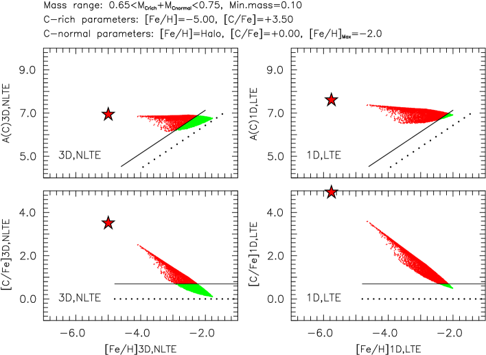
Figure 9: Toy model simulations assuming 3D,NLTE (left) and 1D,LTE (right) adopting a C-rich population with model [Fe/H] = –5.0 and [C/Fe] = +3.5 (represented by the red star symbol in each panel). The upper and lower panels present $A$(C) and [C/Fe] vs. [Fe/H], respectively, for the composite model population. The full and dotted lines refer to the [C/Fe] = +0.7 and 0.0 loci, respectively, while green and red symbols represent stars with [C/Fe] below and above +0.7 dex.

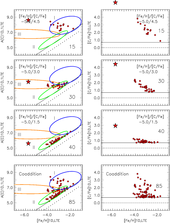
Figure 11: Toy model simulations for $A$(C)_1D,LTE (left) and [C/Fe]_1D,LTE (right) vs. [Fe/H]_1D,LTE, respectively. The upper three rows present results obtained with the adopted [Fe/H]/[C/Fe] pairs for the C-rich population shown in each row, while the bottom row contains the superset of the above upper three panels. The isolated number indicates the number of stars plotted in each panel.

Using these concepts we attempt to learn only about the regions of the $A$(C) and [C/Fe] vs. [Fe/H] planes that are occupied by the putative composite stars, and emphasize that these results should be seen as a zeroth-order approximation. The first assumption is that merging occurs between between clouds of random mass (say M_C-rich and M_C-normal) adopting a Salpter mass function, one from each of the two parent populations, to form a composite CEMP-no star in the currently observable mass range 0.65 – 0.75 M/M_⊙. We implicitly assume that there are reservoirs of gas having the required masses in the two parent populations, and that all of the merging material is used to produce a well-mixed composite star, without mass loss. We then determine the chemical abundances of carbon and iron of each of the coalescing gas clouds. For the C-rich component we adopt a representative pair of values (e.g., [Fe/H]_3D,NLTE = –5.0, and [C/Fe]_3D,NLTE = +3.0). For the cloud from the C-normal population we determine [Fe/H]_3D,NLTE at random from the modified Yong et al. (2013b) MDF over the range –4.0 $<$ [Fe/H]_3D,NLTE $<$ –2.0, and assume [C/Fe]_3D,NLTE = 0.0. Given M_C-rich and M_C-normal, and these chemical abundances for the two clouds, the abundances of the composite star follow. We emphasize that with this approach we seek only to reproduce the observations of the CEMP-no stars with [Fe/H] $>$ –4.0 in Figure 4. The results of a number of simulations are shown in Figures 9 – 11.

Figure 9 pertains to a C-rich parent population having [Fe/H] = –5.0 and [C/Fe] = +3.5, which coalesces with C-normal halo clouds as postulated above. On the left are the computed model results, labeled 3D,NLTE on the assumption that 3D,NLTE observational data would re-produce these results. On the right, labeled 1D,LTE, are the results when the model values are reverse engineered to produce values that would be obtained by a 1D,LTE analysis. The star symbols refer to the adopted values of the C-rich population, while the small symbols represent the composite model results. Figure 10 presents a considerably smaller carbon abundance of the C-rich parent population, with [Fe/H] = –5.0 and [C/Fe] = +1.5, which lead to considerably different abundance distributions compared with the simulation in Figure 9.

In Section 7.1, we noted that the distribution of CEMP-no stars in Figure 4 is obviously non-uniform, leading Yoon et al. (2016) to identify two groups of CEMP-no stars. In Figure 11, we present a comparison of our model results, which contains three simulations and their coaddition, with the Yoon et al. (2016) Groups I, II, and III boundaries – which we recall were defined in this plane. In the figure, simulated $A$(C)_1D,LTE (left) and [C/Fe]_1D,LTE (right) values are plotted as a function of [Fe/H]_1D,LTE, where the format is similar to that of our Figure 4. In the upper left of each of the uppermost three rows in the figure are the assumed [Fe/H]/[C/Fe] parameters of the C-rich population, and assuming these are also the 3D,NLTE values of that population, the large red star symbols represent the corresponding 1D,LTE values. The results of the coalescence model are presented as small red circles, the number of which is given by the isolated number in each of these panels.

Only one parameter, [C/Fe] of the C-rich population, changes among the top three rows of the figure – from +4.5 to +3.0, to +1.5; and at least to first approximation, one can see a reasonable reproduction of the Yoon et al. Groups I, III, and II, respectively, in our Figure 4, proceeding from top towards bottom. Finally, the bottom row of the figure presents the simple co-addition of the data in the upper three rows, and should be compared with the uppermost row of Figure 4.

Perhaps the most interesting feature of the figure is that in the left column ($A$(C) vs. [Fe/H]) the morphology of the distribution of coalesced stars in the top panel ([C/Fe]_C-rich = +4.5), which is similar to that of Yoon et al. (2016) Group III, has changed in the second panel from the bottom ([C/Fe]_C-rich = +1.5) to that of Yoon et al. (2016) Group II. This suggests that the morphology of the CEMP-no stars in this plane is determined by the distribution of carbon in the C-rich cloud population.

We regard the agreement between the model and the observational data as encouraging, given the ad hoc nature and simplicity of the assumptions of the model.

9 Summary and Desiderata

In Sections 3 – 6 we applied literature-based 3D,NLTE corrections to 1D,LTE Fe I iron and CH-based carbon abundances for stars with [Fe/H]_1D,LTE $<$ –2.0, with a view to obtaining a better understanding of the nature and origin of the CEMP-no stars and what they have to tell us about the most iron-poor ([Fe/H] $<$ –4.5) C-rich stars and their relationship to and interaction with the majority iron-poor ([Fe/H] $>$ –4.0), carbon-normal halo population. Bootstrapping from carbon abundances based on 3D,NLTE analysis of the infrared high-excitation C I lines in the range –3.3 $<$ [Fe/H] $<$ –2.0, we showed that although it is not currently possible to theoretically determine NLTE corrections for the CH molecule, the 3D,NLTE corrections are very likely not smaller (absolutely) than the 3D,LTE values. As emphasized by Asplund (2005), the resulting corrections are very large. For example, for the Yoon et al. (2016) compilation of C-rich stars, if one adopts [C/Fe] $>$ +0.7 as a basic requirement of a CEMP-no star, the fraction of CEMP-no stars in the range –4.5 $<$ Fe/H] $<$ –3.0 drops from the 1D,LTE result of 0.30 to the 3D,NLTE value of 0.12.

• In Section 4.2, we found a large number of C-normal stars below [C/Fe]_3D,NLTE $\;\buildrel<\over{\sim}\;$ 0.0 for which the (CH-based) mean [C/Fe]_3D,NLTE abundance is $\langle$[C/Fe]_3D,NLTE$\rangle$ = –0.42 (82 objects), surprisingly low compared with the result of [C/Fe]_3D,NLTE $\sim$ +0.1 based on high-excitation C I lines in metal-poor dwarfs reported by Amarsi et al. (2019). This might be attributed to the fact that the present sample is dominated by giants. That is, for giants in the present sample we find $\langle$[C/Fe]_3D,NLTE$\rangle$ = –0.49 (61 stars) and for dwarfs $\langle$[C/Fe]_3D,NLTE$\rangle$ = –0.24 (21 stars). Also, analysis of C-normal dwarfs in our Table 3 finds $\langle$[C/Fe]_3D,NLTE$\rangle$ = –0.18 (21 stars).

  Perhaps the 1D,LTE values for the giants have been underestimated. Alternatively, we noted that Gallagher et al. (2016) have reported that 3D CH-based carbon abundances are a function of $A$(C). While it could be a massive undertaking, it would be interesting to further investigate parameter space to better understand this effect.

• It may be suggested that 1D,LTE [C/Fe] abundances are no longer of use. We would counter that this would be premature, and are of the view that while comprehensive 3D,NLTE investigations of parameter space are required, further 1D,LTE surveys are important to discover further objects in order to constrain and calibrate the 3D,NLTE predictions.

It was noted in Section 4 that the change of CEMP-no status applies to the Yoon et al. Group II, CEMP-no stars, and not to their C-richer Group III counterparts. An important example of the Group II effect of the corrections on 1D, LTE CH based carbon abundances is the status change of the three Group II classic metal-poor ([Fe/H] $\sim$ –3.0) stars CD $-24^{\circ}\,17504$, G64-12, and G64-37, for which $\langle$[C/Fe]_1D,LTE$\rangle$ = 1.1 and $\langle$[C/Fe]_3D,NLTE$\rangle$ = 0.3 (Section 4.3). In Section 7.1, a second enigmatic result for Group II objects arose in the discussion of 1D,LTE abundances of Na, Mg, and Al (which show large overabundances in the CEMP-no stars) where we found for the Group II stars that while variations in the abundance histograms of these elements were seen in the abundance range [C/Fe]_1D,LTE $>$ +1.0, the effect is not so evident for stars with +0.7 $<$ [C/Fe]_1D,LTE $<$ +1.0.

We also discussed the existence of a $\sim$15% component of CEMP-no stars in the Yoon et al. Group I of CEMP stars, which is comprised principally of CEMP-s stars. In this subgroup of CEMP-no stars we found that the [Sr/Ba]_1D,LTE values are larger than those of the majority of the CEMP-s stars.

• Further work is needed to investigate to what extent the stars in this CEMP-no subgroup may be binary and/or the progeny of spinstars.

Finally, we presented a toy model that seeks to describe the formation of CEMP-no stars in the abundance range –4.0 $\;\buildrel<\over{\sim}\;$ [Fe/H] $\;\buildrel<\over{\sim}\;$ –2.0 in terms of the coalescence of pre-stellar clouds of the two populations that followed the chemical enrichment by the first zero-heavy-element stars, that is, the C-rich, hyper-metal-poor population and the C-normal, extremely-metal-poor, halo stars having [Fe/H] $\;\buildrel>\over{\sim}\;$ –4.0. The simplicity of the model, and the uncertainty of the Fe and C abundance distributions and mass function of the hyper-metal-poor population notwithstanding, the model produces abundance behavior in the $A$(C)_1D,LTE and [C/Fe]_1D,LTE vs. [Fe/H]_1D,LTE planes not unlike that seen in the Yoon et al. (2016) Groups I, II, and III.

• A more rigorous approach to this simple coalescence model would seem worthwhile.

10 APPENDIX: THE 14 MOST IRON-POOR STARS

In Table 6, we present details for the 14 iron-poor stars currently known to have [Fe/H] $<$ –4.5. Columns (1) – (3) contain starname and coordinates, columns (4) – (6) present atmospheric parameters $T_{\rm eff}$, $\log g$, and [Fe/H], column (7) contains [C/Fe], and source information is presented in the final column. In this table the abundances assume 1D,LTE.

Figure 1: The dependence of $A$(C)_1D,LTE, [C/Fe]_1D,LTE, and the generalized histogram of carbon abundance (adopting a Gaussion kernel of 0.10 dex), as a function of [Fe/H]_1D,LTE, for CEMP-no and CEMP-s stars (red and grey, respectively), based on the data of Yoon et al. (2016). In the upper two panels the full line correspond to [C/Fe] = +0.7, the Aoki et al. (2007) boundary between CEMP and C-normal stars, while the dotted line is the [C/Fe] = 0.0 locus.

Figure 4: Carbon vs. iron abundances for CEMP-no (red symbols) and CEMP-s (grey symbols) stars as a function of 1D, 3D, LTE, and NLTE, to demonstrate how the distributions of C and Fe abundances depend on the underlying assumptions of the model atmosphere analysis. The color for each individual star is as determined in the 1D,LTE uppermost panels (a and b). Data are taken from Yoon et al. (2016) and our Table 4. In all panels the thin full and dotted horizontal and inclined lines refer to [C/Fe] = +0.7 and 0.0 loci. The blue, green, and orange ellipses in the top-left panel delineate the Yoon et al. Groups I, II, and III, respectively, while the horizontal orange and light blue lines (truncated by C/Fe] = +1.0 loci) represent the “high carbon band” (orange) and “low carbon band” (light blue) of Spite et al. (2013), Bonifacio et al. (2015, 2018), and Caffau et al. (2018).

Figure 6: Metallicity distribution function (left) and CEMP-no fraction (right) (Gaussian histograms with kernel 0.3 dex) as a function of [Fe/H]_1D,LTE (top), [Fe/H]_3D,LTE (middle), and [Fe/H]_3D,NLTE (bottom). See text for details.

Figure 8: [Sr/Ba]_1D,LTE vs. [Fe/H]_1D,LTE. Red star symbols and circles represent Group I, CEMP-no and Group III, CEMP-no stars, respectively, while grey circles stand for Group I CEMP-s stars.

Figure 10: Toy model simulations assuming 3D,NLTE (left) and 1D,LTE (right) adopting a C-rich population with model [Fe/H] = –5.0 and [C/Fe] = +1.5. The format is the same as in Figure 9, while the model assumes a considerably lower value of [C/Fe] for the C-rich population than in Figure 9.

Table 1: Major Milestones in the Study of CEMP-no Stars

Milestone	Authors
Discovery of very metal-poor stars ([Fe/H]$<$ –2.0) with anomalously strong CH $\lambda$4300 Å features	1
High dispersion abundance analyses reveal distinct C-rich subclasses	2,3,4,5,6
Taxonomy: [C/Fe]CEMP $>$ +0.7; and subclasses CEMP-r, CEMP-s, CEMP-r/s, and CEMP-no	7,8,9
Taxonomy: Many CEMP-no stars have large supersolar abundances of N, O, Na, Mg, and Al	10,11
relative to Fe, but not of the heavy-neutron-capture elements (in particular, [Ba/Fe] $<$ 0.)
Taxonomy: Two distinct peaks in the [Fe/H] and $A$(C) histograms, populated principally by CEMP-no and CEMP-s stars	10,12,13,14,15
Taxonomy: Essentially all CEMP stars with [Fe/H]$\;\buildrel<\over{\sim}\;$–3.3 belong to the CEMP-no subclass	10,12
Taxonomy: Two subgroups of CEMP-no stars exist in $A$(C)–[Fe/H] space	16
For CEMP-no stars, [C/Fe] increases strongly as [Fe/H] decreases	17
Discovery of C-rich stars having [Fe/H]$<$ –5.5 (assumed to be CEMP-no stars)	18,19,20
14 halo stars currently known to have [Fe/H]$<$ –4.5. At least 11 of them are C-rich	11,21,22,23,24,25,26
CEMP-no main-sequence-turnoff stars with [Fe/H] $<$ –4.0 have A(Li) $<$ 2.0	14,27
The earliest two observed stellar populations formed by cooling of C-rich and C-normal clouds	10,28,29,30
Suggested origin of CEMP-no enrichment: mixing and fallback stellar models (in minihalos)	31,32,33,(34)
Suggested origin of CEMP-no enrichment: spinstars	35,36,37
Suggested origin of CEMP-no enrichment: mixing and fallback + spinstars	38
Suggested origin of CEMP-no enrichment: binarity	39
Radial velocity monitoring supports CEMP-no binary fraction similar to that of C-normal halo stars	10,40,41
Most recent radial velocity monitoring reports that CEMP-no binary fraction is larger than C-normal halo star value	42
The fraction of CEMP-no stars increases as [Fe/H] decreases, and as Galactocentric distance increases	43,44,45
The ratio of CEMP-no to CEMP-s stars reported to increase with increasing Galactocentric distance	46,47,48
CEMP-no stars exist in the Milky Way’s dwarf ultra-faint galaxy satellites Bootes I and Segue 1	49,50
Discovery of Damped Lyman-$\alpha$ Systems with enhanced [C/Fe] in quasar Ly$\alpha$ forests	51,52,53
Discussion of CEMP-no stars within the framework of the formation of the first galaxies	54,55,56

Table 2: Literature [Fe/H] and $A$(C) values

Star	$T_{\rm eff}$	$\log g$	[Fe/H]	[Fe/H]	[Fe/H]	[Fe/H]	$A$(C)	$A$(C)	Source
	(K)		1D,LTE	1D,NLTE	3D,LTE	3D,NLTE	1D,LTE	3D,LTE
(1)	(2)	(3)	(4)	(5)	(6)	(7)	(8)	(9)	(10)
HD 84937	6356	4.1	$-$2.19	$-$2.02	$-$2.24	$-$1.90	…	…	1
HD 122563	4587	1.6	$-$2.87	$-$2.78	$-$2.94	$-$2.70	…	…	1
HD 122563	4600	1.6	$-$2.75	…	$-$2.83	…	5.28	5.33	2
HD 140283	5591	3.6	$-$2.68	$-$2.49	$-$2.79	$-$2.34	…	…	1
G 64-12	6435	4.3	$-$3.21	$-$2.98	$-$3.32	$-$2.87	…	…	1
CD $-$38${}^{\circ}\,245$	4700	2.0	$-$4.28	$-$4.03	…	…	…	…	3
CS 22949-037	4800	1.9	$-$3.99	$-$3.48	…	…	…	…	3
CS 30336-049	4685	1.4	$-$4.21	$-$3.91	…	…	…	…	3
HE 0057$-$5959	5200	2.8	$-$4.28	$-$3.83	…	…	…	…	3
HE 0107$-$5240	5130	2.2	$-$5.44	…	$-$5.67	…	6.81	5.81	4
HE 0107$-$5240	5050	2.3	$-$5.47	$-$4.72	…	…	…	…	3
HE 0233$-$0343	6020	3.4	$-$4.44	$-$3.99	…	…	…	…	3
HE 0557$-$4840	4800	2.4	$-$4.86	$-$4.48	…	…	…	…	3
HE 1310$-$0536	5000	1.9	$-$4.25	$-$3.77	…	…	…	…	3
HE 1327$-$2326	6190	3.9	$-$5.71	…	$-$5.95	…	6.84	6.13	4,5
HE 1327$-$2326	6130	3.7	$-$5.82	$-$5.16	…	…	…	…	3
HE 1424$-$0241	5140	2.8	$-$4.19	$-$3.73	…	…	…	…	3
HE 2139$-$5432	5270	3.2	$-$4.00	$-$3.52	…	…	…	…	3
HE 2239$-$5019	6000	3.5	$-$4.18	$-$3.76	…	…	…	…	3
SD 0140+2344	5600	4.6	$-$4.09	$-$3.83	…	…	…	…	3
SD 1029+1729	5811	4.0	$-$4.63	$-$4.23	…	…	…	…	3
SD 1143+2020	6240	4.0	$-$3.15	…	…	…	8.10	7.40	6
SD 1204+1201	5350	3.3	$-$4.39	$-$3.91	…	…	…	…	3
SD 1313$-$0019	5100	2.7	$-$5.02	$-$4.41	…	…	…	…	3
SD 1742+2531	6345	4.0	$-$4.82	$-$4.34	…	…	…	…	3
SD 2209$-$0028	6440	4.0	$-$3.97	$-$3.65	…	…	…	…	3
5131/2.2/$-$1.0	5131	2.2	$-$1.00	…	…	…	7.52	7.40	7
5035/2.2/$-$2.0	5035	2.2	$-$2.00	…	…	…	6.52	6.30	7
5128/2.2/$-$3.0	5128	2.2	$-$3.00	…	…	…	5.52	4.80	7
C-normal dwarfs	5900–6500	4.0–4.5	$-$3.00	…	…	…	5.95	5.55	8
CEMP-no dwarfs	5900–6500	4.0–4.5	$-$3.00	…	…	…	6.80	6.50	8

Table 3: Carbon abundances from C I lines and the CH G-band

Star	$T_{\rm eff}$	$\log g$	[Fe/H]	$A$(C I)	$A$(C I)	$A$(CH)	$A$(CH)	$A$(C I)1D,NLTE	$S/N$	Source
	(K)		1D,LTE	1D,LTE	1D,NLTE	1D,LTE	3D,LTE	$-$$A$(CH)3D,LTE
(1)	(2)	(3)	(4)	(5)	(6)	(7)	(8)	(9)	(10)	(11)
HD 84937	6357	4.07	$-$2.11	6.57	6.32	6.56	6.29	0.03	500	1
HD 140283	5849	3.72	$-$2.38	6.31	6.07	6.21	5.89	0.18	470	2
HD 188031	6234	4.16	$-$1.72	6.88	6.67	6.91	6.70	$-$0.03	180	3
HD 215801	6071	3.83	$-$2.28	6.36	6.10	6.46	6.16	$-$0.06	180	3
BD $-$13 3442	6366	3.99	$-$2.69	6.18	5.85	$<$6.16	$<$ 5.79	$>$ 0.06	200	3
CD $-$24 17504	6338	4.32	$-$3.21	5.85	5.55	6.06	5.60	$-$0.05	280	4
CD $-$24 17504	6228	3.90	$-$3.41	5.71	5.45	6.12	5.63	$-$0.18	510	5
CD $-$35 14849	6294	4.26	$-$2.34	6.42	6.17	6.51	6.20	$-$0.03	180	3
CD $-$42 14278	6085	4.39	$-$2.03	6.58	6.41	6.76	6.50	$-$0.09	90	6
CD $-$71 1234	6325	4.18	$-$2.38	6.32	6.07	6.31	5.99	0.08	310	4
G 4-37	6308	4.25	$-$2.45	6.30	6.03	6.46	6.13	$-$0.10	150	4
G 11-44	6178	4.35	$-$2.03	6.62	6.45	6.71	6.45	0.00	120	6
G 13-9	6343	4.01	$-$2.29	6.52	6.22	6.46	6.16	0.06	280	7
G 24-3	6084	4.23	$-$1.62	6.69	6.52	6.86	6.67	$-$0.15	240	8
G 29-23	6194	4.04	$-$1.69	6.86	6.64	6.86	6.66	$-$0.02	200	8
G 48-29	6489	4.25	$-$2.60	6.05	5.76	$<$6.46	$<$6.11	$>$$-$0.35	240	4
G 48-29	6489	4.25	$-$2.60	6.05	5.76	$<$6.31	$<$5.96	$>$$-$0.20	220	9
G 59-27	6272	4.23	$-$1.93	6.85	6.63	6.86	6.62	0.01	210	4
G 64-12	6435	4.26	$-$3.24	5.71	5.30	6.16	5.70	$-$0.40	700	10
G 64-12	6463	4.26	$-$3.29	5.71	5.30	6.21	5.74	$-$0.44	700	11
G 64-37	6570	4.40	$-$3.11	5.75	5.34	6.36	5.92	$-$0.58	700	10
G 64-37	6570	4.40	$-$3.11	5.75	5.34	6.44	6.00	$-$0.66	700	11
G 126-52	6396	4.20	$-$2.21	6.46	6.21	6.46	6.17	0.04	270	4
G 166-54	6407	4.28	$-$2.58	6.07	5.75	6.16	5.81	$-$0.06	240	4
G 186-26	6417	4.42	$-$2.54	6.19	5.91	6.32	5.98	$-$0.07	110	3
LP 635-14	6367	4.11	$-$2.39	6.43	6.14	6.46	6.14	0.00	250	4
LP 651-4	6371	4.20	$-$2.63	6.12	5.81	6.21	5.85	$-$0.04	240	4

Table 4: $T_{\rm eff}$, $\log g$, and carbon and iron abundances for eight recently reported CEMP-no stars

Star	$T_{\rm eff}$	$\log g$	[Fe/H]	[C/Fe]	$A$(C)	[Ba/Fe]	Source
	(K)		1D,LTE	1D,LTE	1D,LTE
(1)	(2)	(3)	(4)	(5)	(6)	(7)	(8)
G 64-12	6463	4.26	$-$3.29	+1.07	6.21	$-$0.06	1
G 64-37	6570	4.40	$-$3.11	+1.12	6.44	$-$0.35	1
SD 1341+4741	5450	2.50	$-$3.20	+1.00	6.23	$-$0.73	2
Bootes I-119	4770	1.40	$-$3.33	+2.42	7.52	$-$1.00	3,4
Pisces II-10694	4130	0.80	$-$2.60	+1.58	7.48	$-$1.10	5
Segue 1-7	4960	1.90	$-$3.52	+2.38	7.29	$<-$0.96	6
Segue 1 SD 1006+1602	5484	3.30	$-$3.60	+1.20	6.03	$<-$1.87	7
Segue 1 SD 1006+1600	5170	2.50	$-$3.78	+0.91	5.54	$<-$2.25	7

Table 5: Data for 19 CEMP-no, Group I Stars

Star	$T_{\rm eff}$	$\log g$	[Fe/H]	[C/Fe]	$A$(C)	[Ba/Fe]	Binary?	Source
	(K)		1D,LTE	1D,LTE	1D,LTE
(1)	(2)	(3)	(4)	(5)	(6)	(7)	(8)	(9)
CS 22943-201	5970	2.45	$-$2.68	1.90	7.65	$-$0.54	…	1
CS 22957-027	5220	2.65	$-$3.19	2.63	7.87	$-$0.81	Yes	2,3
CS 22958-042	5760	3.55	$-$3.40	2.56	7.59	$-$0.61	…	4,1
CS 29498-043	4440	0.50	$-$3.87	3.06	7.62	$-$0.49	No	3
HE 0100$-$1622	5400	3.00	$-$2.93	2.77	8.27	$-$1.80	…	5
HE 0219$-$1739	4238	0.47	$-$3.09	2.21	7.55	$-$1.39	Yes	3
HE 0405$-$0526	5083	3.86	$-$2.18	0.92	7.17	$-$0.22	No	3
HE 1133$-$0555	5526	1.31	$-$2.40	2.28	8.31	$-$0.58	No	3
HE 1150$-$0428	5208	2.54	$-$3.47	2.39	7.35	$-$0.48	Yes	3
HE 1302$-$0954	5120	2.40	$-$2.25	1.19	7.37	$-$0.53	No	3
HE 1330$-$0354	6257	4.13	$-$2.29	1.01	7.15	$-$0.52	…	6
HE 1410+0213	5000	2.00	$-$2.14	1.92	8.21	$-$0.26	No	3
HE 1456+0230	5664	2.20	$-$3.37	2.37	7.43	$-$0.19	…	7
HE 2202$-$4831	5331	2.95	$-$2.78	2.43	8.08	$-$1.28	…	8
HE 2319$-$5228	4900	1.60	$-$2.60	1.87	7.70	$-$3.00	…	9
SDSS J1422+0031	5200	2.20	$-$3.03	1.71	7.11	$-$1.18	Yes	10
Bootes I-119	4770	1.40	$-$3.33	2.42	7.52	$-$1.00	…	11
Pisces II-10694	4130	0.80	$-$2.60	1.65	7.48	$-$1.10	…	12
Segue 1-7	4960	1.90	$-$3.52	2.38	7.29	$-$0.96	…	13,14

Table 6: The 14 Most Iron-poor Stars

Star	RA2000	Dec2000	$T_{\rm eff}$	$\log g$	[Fe/H]	[C/Fe]	Sources
(1)	(2)	(3)	(4)	(5)	(6)	(7)	(8)
SMSS J0313$-$6708	03 13 00.4	$-$67 08 39.3	5125	2.3	$<$$-$7.30	$>$+4.9	1
SMSS J1605$-$1443	16 05 40.2	$-$14 43 23.1	4850	2.0	$-$6.20	+3.9	2
SDSS J0815+4729	08 15 54.2	+47 29 47.8	6215	4.7	$<$$-$5.80	$>$+5.0	3
HE 1327$-$2326	13 30 06.0	$-$23 41 49.7	6180	3.7	$-$5.66	+4.3	4
SDSS J0023+0307	00 23 14.0	+03 07 58.1	6224	4.8	$<$$-$5.50	$>$+3.2	5
HE 0107$-$5240	01 09 29.2	$-$52 24 34.2	5100	2.2	$-$5.39	+3.7	6
SDSS J1035+0641	10 35 56.1	+06 41 44.0	6262	4.0	$<$$-$5.07	$>$+3.5	7
SDSS J1313$-$0019	13 13 26.9	$-$01 19 41.4	5200	2.6	$-$5.00	$\sim$+3.0	8
SDSS J0929+0238	09 29 12.3	+02 38 17.0	5894	3.7	$-$4.97	+3.9	9
SDSS J1742+2531	17 42 59.7	+25 31 35.9	6345	4.0	$-$4.80	+3.6	10
HE 0557$-$4840	05 58 39.3	$-$48 39 56.8	4900	2.0	$-$4.75	+1.6	11
SDSS J1029+1729	10 29 15.2	+17 29 28.0	5811	4.0	$-$4.73	$<$+0.9	12
HE 0233$-$0343	02 36 29.7	$-$03 30 06.0	6100	3.4	$-$4.68	+3.5	13
Pristine_221.8781+9.7844	14 47 30.7	+09 47 03.7	5792	3.5	$-$4.66	$<$+1.8	14

References

- Aguado et al. (2018a) Aguado, D. S., Allende Prieto, C., González Hernández, J. I., & Rebolo, R. 2018a, ApJ, 854, L34
- Aguado et al. (2018b) Aguado, D. S., González Hernández, J. I., Allende Prieto, C., & Rebolo, R. 2018b, ApJ, 852, L20
- Aguado et al. (2019) —. 2019, ApJ, 874, L21
- Amarsi et al. (2016) Amarsi, A. M., Lind, K., Asplund, M., Barklem, P. S., & Collet, R. 2016, MNRAS, 463, 1518
- Amarsi et al. (2019) Amarsi, A. M., Nissen, P. E., Asplund, M., Lind, K., & Barklem, P. S. 2019, arXiv:1901.03592
- Aoki (2010) Aoki, W. 2010, in IAU Symposium, Vol. 265, Chemical Abundances in the Universe: Connecting First Stars to Planets, ed. K. Cunha, M. Spite, & B. Barbuy, 111
- Aoki et al. (2007) Aoki, W., Beers, T. C., Christlieb, N., et al. 2007, ApJ, 655, 492
- Aoki et al. (2013) Aoki, W., Beers, T. C., Lee, Y. S., et al. 2013, AJ, 145, 13
- Aoki et al. (2006) Aoki, W., Frebel, A., Christlieb, N., et al. 2006, ApJ, 639, 897
- Aoki et al. (2002) Aoki, W., Norris, J. E., Ryan, S. G., Beers, T. C., & Ando, H. 2002, PASJ, 54, 933
- Arentsen et al. (2018) Arentsen, A., Starkenburg, E., Shetrone, M. D., et al. 2018, ArXiv:1811.01975
- Asplund (2005) Asplund, M. 2005, ARA&A, 43, 481
- Bandyopadhyay et al. (2018) Bandyopadhyay, A., Sivarani, T., Susmitha, A., et al. 2018, ApJ, 859, 114
- Barbuy et al. (1997) Barbuy, B., Cayrel, R., Spite, M., et al. 1997, A&A, 317, L63
- Barklem et al. (2011) Barklem, P. S., Belyaev, A. K., Guitou, M., et al. 2011, A&A, 530, A94
- Barklem et al. (2005) Barklem, P. S., Christlieb, N., Beers, T. C., et al. 2005, A&A, 439, 129
- Becker et al. (2012) Becker, G. D., Sargent, W. L. W., Rauch, M., & Carswell, R. F. 2012, ApJ, 744, 91
- Beers & Christlieb (2005) Beers, T. C., & Christlieb, N. 2005, ARA&A, 43, 531
- Beers et al. (1992) Beers, T. C., Preston, G. W., & Shectman, S. A. 1992, AJ, 103, 1987
- Bonifacio et al. (2015) Bonifacio, P., Caffau, E., Spite, M., et al. 2015, A&A, 579, A28
- Bonifacio et al. (2018) —. 2018, A&A, 612, A65
- Bonifacio et al. (1998) Bonifacio, P., Molaro, P., Beers, T. C., & Vladilo, G. 1998, A&A, 332, 672
- Caffau et al. (2012) Caffau, E., Bonifacio, P., François, P., et al. 2012, arXiv 1203.2607
- Caffau et al. (2016) Caffau, E., Bonifacio, P., Spite, M., et al. 2016, A&A, 595, L6
- Caffau et al. (2018) Caffau, E., Gallagher, A. J., Bonifacio, P., et al. 2018, A&A, 614, A68
- Carney & Peterson (1981) Carney, B. W., & Peterson, R. C. 1981, ApJ, 245, 238
- Carollo et al. (2012) Carollo, D., Beers, T. C., Bovy, J., et al. 2012, ApJ, 744, 195
- Carollo et al. (2014) Carollo, D., Freeman, K., Beers, T. C., et al. 2014, ApJ, 788, 180
- Carswell et al. (2012) Carswell, R. F., Becker, G. D., Jorgenson, R. A., Murphy, M. T., & Wolfe, A. M. 2012, MNRAS, 422, 1700
- Castelli & Kurucz (2003) Castelli, F., & Kurucz, R. L. 2003, in IAU Symp. 210, Modelling of Stellar Atmospheres, ed. N. Piskunov, W. W. Weiss, & D. F. Gray (San Francisco, CA: ASP), A20
- Chiaki et al. (2017) Chiaki, G., Tominaga, N., & Nozawa, T. 2017, MNRAS, 472, L115
- Christlieb et al. (2002) Christlieb, N., Bessell, M. S., Beers, T. C., et al. 2002, Nature, 419, 904
- Christlieb et al. (2004) Christlieb, N., Gustafsson, B., Korn, A. J., et al. 2004, ApJ, 603, 708
- Cohen et al. (2008) Cohen, J. G., Christlieb, N., McWilliam, A., et al. 2008, ApJ, 672, 320
- Cohen et al. (2013) Cohen, J. G., Christlieb, N., Thompson, I., et al. 2013, ApJ, 778, 56
- Collet et al. (2006) Collet, R., Asplund, M., & Trampedach, R. 2006, ApJ, 644, L121
- Collet et al. (2007) —. 2007, A&A, 469, 687
- Collet et al. (2018) Collet, R., Nordlund, Å., Asplund, M., Hayek, W., & Trampedach, R. 2018, MNRAS, 475, 3369
- Cooke et al. (2012) Cooke, R., Pettini, M., & Murphy, M. T. 2012, MNRAS, 425, 347
- Cooke et al. (2011) Cooke, R., Pettini, M., Steidel, C. C., Rudie, G. C., & Jorgenson, R. A. 2011, MNRAS, 412, 1047
- Cooke & Madau (2014) Cooke, R. J., & Madau, P. 2014, ApJ, 791, 116
- Demarque et al. (2004) Demarque, P., Woo, J., Kim, Y., & Yi, S. K. 2004, ApJS, 155, 667
- Dobrovolskas et al. (2013) Dobrovolskas, V., Kučinskas, A., Steffen, M., et al. 2013, A&A, 559, A102
- Elmegreen (2002) Elmegreen, B. G. 2002, ApJ, 564, 773
- Ezzeddine et al. (2017) Ezzeddine, R., Frebel, A., & Plez, B. 2017, ApJ, 847, 142
- Fabbian et al. (2009) Fabbian, D., Nissen, P. E., Asplund, M., Pettini, M., & Akerman, C. 2009, A&A, 500, 1143
- Frebel et al. (2005) Frebel, A., Aoki, W., Christlieb, N., et al. 2005, Nature, 434, 871
- Frebel et al. (2015) Frebel, A., Chiti, A., Ji, A. P., Jacobson, H. R., & Placco, V. M. 2015, ApJ, 810, L27
- Frebel et al. (2006) Frebel, A., Christlieb, N., Norris, J. E., et al. 2006, ApJ, 652, 1585
- Frebel et al. (2008) Frebel, A., Collet, R., Eriksson, K., Christlieb, N., & Aoki, W. 2008, ApJ, 684, 588
- Frebel et al. (2019) Frebel, A., Ji, A. P., Ezzeddine, R., et al. 2019, ApJ, 871, 146
- Frebel & Norris (2015) Frebel, A., & Norris, J. E. 2015, ARA&A, 53, 631
- Frebel et al. (2007) Frebel, A., Norris, J. E., Aoki, W., et al. 2007, ApJ, 658, 534
- Frebel et al. (2014) Frebel, A., Simon, J. D., & Kirby, E. N. 2014, ApJ, 786, 74
- Frischknecht et al. (2010) Frischknecht, U., Hirschi, R., Meynet, G., et al. 2010, A&A, 522, A39
- Frischknecht et al. (2012) Frischknecht, U., Hirschi, R., & Thielemann, F.-K. 2012, A&A, 538, L2
- Gallagher et al. (2016) Gallagher, A. J., Caffau, E., Bonifacio, P., et al. 2016, A&A, 593, A48
- Gilmore et al. (2013) Gilmore, G., Norris, J. E., Monaco, L., et al. 2013, ApJ, 763, 61
- Hansen et al. (2019) Hansen, C. J., Hansen, T. T., Koch, A., et al. 2019, arXiv:1901.05968
- Hansen et al. (2016a) Hansen, C. J., Nordström, B., Hansen, T. T., et al. 2016a, A&A, 588, A37
- Hansen et al. (2014) Hansen, T., Hansen, C. J., Christlieb, N., et al. 2014, ApJ, 787, 162
- Hansen et al. (2015) —. 2015, ApJ, 807, 173
- Hansen et al. (2016b) Hansen, T. T., Andersen, J., Nordström, B., et al. 2016b, A&A, 586, A160
- Heger & Woosley (2010) Heger, A., & Woosley, S. E. 2010, ApJ, 724, 341
- Hollek et al. (2011) Hollek, J. K., Frebel, A., Roederer, I. U., et al. 2011, ApJ, 742, 54
- Ito et al. (2013) Ito, H., Aoki, W., Beers, T. C., et al. 2013, ApJ, 773, 33
- Iwamoto et al. (2005) Iwamoto, N., Umeda, H., Tominaga, N., Nomoto, K., & Maeda, K. 2005, Science, 309, 451
- Jacobson & Frebel (2015) Jacobson, H. R., & Frebel, A. 2015, ApJ, 808, 53
- Keller et al. (2014) Keller, S. C., Bessell, M. S., Frebel, A., et al. 2014, Nature, 506, 463
- Lai et al. (2011) Lai, D. K., Lee, Y. S., Bolte, M., et al. 2011, ApJ, 738, 51
- Lee et al. (2017) Lee, Y. S., Beers, T. C., Kim, Y. K., et al. 2017, ApJ, 836, 91
- Lee et al. (2013) Lee, Y. S., Beers, T. C., Masseron, T., et al. 2013, AJ, 146, 132
- Lugaro et al. (2012) Lugaro, M., Karakas, A. I., Stancliffe, R. J., & Rijs, C. 2012, ApJ, 747, 2
- Maeder & Meynet (2015) Maeder, A., & Meynet, G. 2015, A&A, 580, A32
- Maeder et al. (2015) Maeder, A., Meynet, G., & Chiappini, C. 2015, A&A, 576, A56
- Masseron et al. (2014) Masseron, T., Plez, B., Van Eck, S., et al. 2014, A&A, 571, A47
- Matsuno et al. (2017) Matsuno, T., Aoki, W., Suda, T., & Li, H. 2017, PASJ, 69, 24
- McWilliam et al. (1995) McWilliam, A., Preston, G. W., Sneden, C., & Searle, L. 1995, AJ, 109, 2757
- Meynet et al. (2006) Meynet, G., Ekström, S., & Maeder, A. 2006, A&A, 447, 623
- Nomoto et al. (2013) Nomoto, K., Kobayashi, C., & Tominaga, N. 2013, ARA&A, 51, 457
- Nordlander et al. (2017) Nordlander, T., Amarsi, A. M., Lind, K., et al. 2017, A&A, 597, A6
- Nordlander et al. (2019) Nordlander, T., Bessell, M. S., Da Costa, G. S., et al. 2019, arXiv:1904.07471
- Norris et al. (2007) Norris, J. E., Christlieb, N., Korn, A. J., et al. 2007, ApJ, 670, 774
- Norris et al. (1997a) Norris, J. E., Ryan, S. G., & Beers, T. C. 1997a, ApJ, 488, 350
- Norris et al. (1997b) —. 1997b, ApJ, 489, L169
- Norris et al. (2013) Norris, J. E., Yong, D., Bessell, M. S., et al. 2013, ApJ, 762, 28
- Norris et al. (2010) Norris, J. E., Yong, D., Gilmore, G., & Wyse, R. F. G. 2010, ApJ, 711, 350
- Placco et al. (2016a) Placco, V. M., Beers, T. C., Reggiani, H., & Meléndez, J. 2016a, ApJ, 829, L24
- Placco et al. (2016b) Placco, V. M., Frebel, A., Beers, T. C., et al. 2016b, ApJ, 833, 21
- Placco et al. (2014) Placco, V. M., Frebel, A., Beers, T. C., & Stancliffe, R. J. 2014, ApJ, 797, 21
- Plez & Cohen (2005) Plez, B., & Cohen, J. G. 2005, A&A, 434, 1117
- Preston & Sneden (2001) Preston, G. W., & Sneden, C. 2001, AJ, 122, 1545
- Roederer et al. (2014) Roederer, I. U., Preston, G. W., Thompson, I. B., et al. 2014, AJ, 147, 136
- Rossi et al. (1999) Rossi, S., Beers, T. C., & Sneden, C. 1999, in Astronomical Society of the Pacific Conference Series, Vol. 165, The Third Stromlo Symposium: The Galactic Halo, ed. B. K. Gibson, R. S. Axelrod, & M. E. Putman, 264
- Ryan et al. (2005) Ryan, S. G., Aoki, W., Norris, J. E., & Beers, T. C. 2005, ApJ, 635, 349
- Ryan et al. (1991) Ryan, S. G., Norris, J. E., & Bessell, M. S. 1991, AJ, 102, 303
- Sarmento et al. (2017) Sarmento, R., Scannapieco, E., & Pan, L. 2017, ApJ, 834, 23
- Schneider et al. (2012) Schneider, R., Omukai, K., Bianchi, S., & Valiante, R. 2012, MNRAS, 419, 1566
- Sharma et al. (2018) Sharma, M., Theuns, T., Frenk, C. S., & Cooke, R. J. 2018, MNRAS, 473, 984
- Sivarani et al. (2006) Sivarani, T., Beers, T. C., Bonifacio, P., et al. 2006, A&A, 459, 125
- Sneden (1973) Sneden, C. 1973, ApJ, 184, 839
- Sneden et al. (1994) Sneden, C., Preston, G. W., McWilliam, A., & Searle, L. 1994, ApJ, 431, L27
- Sobeck et al. (2011) Sobeck, J. S., Kraft, R. P., Sneden, C., et al. 2011, AJ, 141, 175
- Spite et al. (2013) Spite, M., Caffau, E., Bonifacio, P., et al. 2013, A&A, 552, A107
- Spite et al. (2018) Spite, M., Spite, F., François, P., et al. 2018, A&A, 617, A56
- Starkenburg et al. (2018) Starkenburg, E., Aguado, D. S., Bonifacio, P., et al. 2018, MNRAS, 481, 3838
- Starkenburg et al. (2014) Starkenburg, E., Shetrone, M. D., McConnachie, A. W., & Venn, K. A. 2014, MNRAS, 441, 1217
- Suda et al. (2004) Suda, T., Aikawa, M., Machida, M., Fujimoto, M., & Iben, I. 2004, ApJ, 611, 476
- Takahashi et al. (2014) Takahashi, K., Umeda, H., & Yoshida, T. 2014, ApJ, 794, 40
- Umeda & Nomoto (2003) Umeda, H., & Nomoto, K. 2003, Nature, 422, 871
- Yong et al. (2013a) Yong, D., Norris, J. E., Bessell, M. S., et al. 2013a, ApJ, 762, 26
- Yong et al. (2013b) —. 2013b, ApJ, 762, 27
- Yoon et al. (2016) Yoon, J., Beers, T. C., Placco, V. M., et al. 2016, ApJ, 833, 20