Transport and Phonon Damping in ⁴He

Abstract

The dynamic structure function $S(k,\omega)$ informs about the dispersion and damping of excitations. We have recently (Phys. Rev. B 97, 184520 (2018)) compared experimental results for $S(k,\omega)$ from high-precision neutron scattering experiments and theoretical results using the “dynamic many-body theory” (DMBT), showing excellent agreement over the whole experimentally accessible pressure regime. This paper focuses on the specific aspect of the propagation of low-energy phonons. We report calculations of the phonon mean-free path and phonon life time in liquid ⁴He as a function of wave length and pressure. Historically, the question was of interest for experiments of quantum evaporation. More recently, there is interest in the potential use of ⁴He as a detector for low-energy dark matter (K. Schulz and Kathryn M. Zurek, Phys. Rev. Lett. 117, 121302 (2016)). While the mean free path of long wave length phonons is large, phonons of intermediate energy can have a short mean free path of the order of $\mu$m. Comparison of different levels of theory indicate that reliable predictions of the phonon mean free path can be made only by using the most advanced many–body method available, namely, DMBT.

1 Introduction

It has been known for a long time MarisRMP -Sridhar87 that low-energy phonons in liquid ⁴He display an anomalous dispersion relation which allows these phonons to decay. Precise neutron scattering measurements of the phonon dispersion in liquid ⁴He skwpress provide the phonon dispersion relation for all experimentally accessible densites with unprecedented accuracy. They confirm the finding of earlier work that the phonon dispersion relation is anomalous up to densities of about $\rho=0.0245$Å^-3. These data agree very well with our recent theoretical results for the dynamics of ⁴He based on time-dependent multiparticle correlations eomIII ; our methods should therefore also be capable of quantitative microscopic predictions for the phonon lifetime. We apply our many-body theory of inelastic scattering, previously applied to scattering off ⁴He droplets dropdyn and the surface of ⁴He hscatt . In the following sections, we briefly review both the theoretical methods used to calculate the relevant ground state properties (Section 2) and the dynamic features (Section 3) of the ⁴He liquid, and the data analysis to obtain accurate values of the phonon dispersion coefficient.

The investigations are, among others, of interest because multiple scattering in superfluid ⁴He has been proposed as a detection mechanism for low-mass dark matter PRL117Zurek -Romani2019 , among other proposed detectors PhysRevLett.119.131802 . Such a detector design requires accurate knowledge of the propagation of low-energy phonons within the medium. In particular, when the phonon dispersion relation is anomalous, phonons are damped and have a finite mean free path.

2 Ground State Structure of ⁴He

Microscopic calculation of properties of many–body systems begin with an accurate calculation of ground–state properties. For ⁴He it is adequate to begin with a non-relativistic Hamiltonian

$$H=-\frac{\hbar^{2}}{2m}\sum_{i}\nabla_{i}^{2}+\sum_{i<j}v(|{\bf r}_{i}-{\bf r}_{j}|)$$ (1)

where the pair-wise interaction $v(r)$ is taken from Aziz et al. AzizII .

The most efficient evaluation of ground state properties is done by the variational Jastrow-Feenberg ansatz for the ground state:

$$\Psi_{0}({\bf r}_{1},\ldots,{\bf r}_{N})=\exp\,\frac{1}{2}\left[\sum_{i<j}u_{2}({\bf r}_{i},{\bf r}_{j})+\sum_{i<j<k}u_{3}({\bf r}_{i},{\bf r}_{j},{\bf r}_{k})\right]\,.$$ (2)

The correlation functions $u_{i}({\bf r}_{1},\dots,{\bf r}_{i})$ are obtained by minimizing the ground state energy $E_{0}$

$$\frac{\delta}{\delta u_{i}({\bf r}_{1},\dots,{\bf r}_{i})}\frac{\bigl{\langle}{\Psi_{0}}\bigr{|}H\bigl{|}{\Psi_{0}}\bigr{\rangle}}{\bigl{\langle}{\Psi_{0}}\big{|}{\Psi_{0}}\bigr{\rangle}}=0\,.$$ (3)

The method is known as Jastrow-Feenberg-Euler-Lagrange (JF-EL) method. The key quantity obtained from such a ground state calculation and used for the calculation of the dynamics is the static structure function $S(k)$. We show in Fig. 1 a comparison of different calculations and experiments.

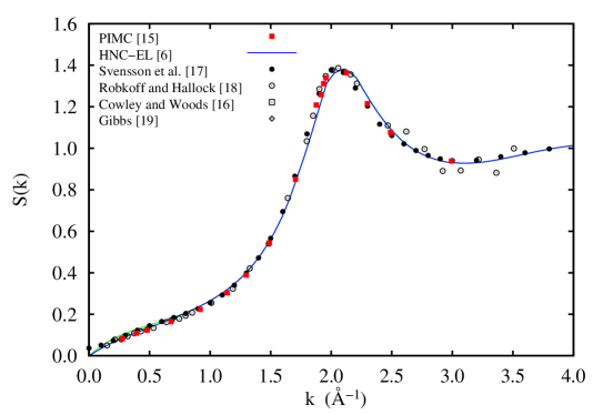
Figure 1: (color online) Static structure function $S(k)$ for ⁴He at equilibrium density. We compare JF-EL, Monte Carlo JordiQFSBook , and experiments CowleyWoods ; svensson ; RoHa ; AndersenRoton . The figure is from Ref. 6.

3 Many-Body Dynamics

Dynamics is treated at the same level as the ground state: We write the dynamic wave function as containing a small, time-dependent component

$$\left|\Psi(t)\right\rangle=e^{-\mathrm{i}E_{0}t/\hbar}\frac{e^{\frac{1}{2}\delta U(t)}\left|\Psi_{0}\right\rangle}{[\langle\Psi_{0}|e^{\frac{1}{2}\delta U^{\dagger}(t)}e^{\frac{1}{2}\delta U(t)}|\Psi_{0}\rangle]^{1/2}}\ ,$$ (4)

where $\bigl{|}{\Psi_{0}}\bigr{\rangle}$ is the ground state, and $\delta U(t)$ is an excitation operator that is written, for the case of bosons, in exactly the same manner as the ground state wave function:

$$\delta U(t)=\sum_{i}\delta u_{1}({\bf r}_{i};t)+\sum_{i<j}\delta u_{2}({\bf r}_{i},{\bf r}_{j};t)+\ldots$$ (5)

The amplitudes $\delta u_{i}({\bf r}_{1},\ldots{\bf r}_{i};t)$ are determined by the time-dependent generalization of the Ritz’ variational principle:

$$\frac{\delta}{\delta u_{i}({\bf r}_{1},\dots{\bf r}_{i};t)}\int\!\!dt\,\langle\,\Psi(t)|H-\mathrm{i}\hbar\partial_{t}|\Psi(t)\rangle=0\,.$$ (6)

Assuming that $\delta U(t)$ is a small perturbation of the ground state correlations, we can linearize the equations of motion for $\delta u_{i}({\bf r}_{i},\dots;t)$, leading to the density–density response function $\chi(k,\omega)$ from which we obtain the dynamic structure function $S(k,\omega)=\Im m\,\chi(k,\omega)$:

$$\chi(q,\omega)=\frac{S(q)}{\hbar\omega-\varepsilon_{\rm F}(q)-\Sigma(q,\hbar\omega)}+\frac{S(q)}{-\hbar\omega-\varepsilon_{\rm F}(q)-\Sigma(q,-\hbar\omega)}\ ,$$ (7)

where $\varepsilon_{\rm F}(k)=\hbar^{2}k^{2}/2mS(k)$ is the Feynman excitation spectrum, and the self-energy is given by an integral equation

$$\Sigma(q,\hbar\omega)=\frac{1}{2}\int\frac{d^{3}k_{1}d^{3}k_{2}}{(2\pi)^{3}\rho}\,\frac{\delta({\bf q}-{\bf k}_{1}-{\bf k}_{2})\left|\tilde{V}_{3}({\bf q};{\bf k}_{1},{\bf k}_{2})\right|^{2}}{\hbar\omega-\varepsilon_{\rm F}(k_{1})-\Sigma(k_{1},\hbar\omega-\varepsilon_{\rm F}(k_{2}))-\varepsilon_{\rm F}(k_{2})-\Sigma(k_{2},\hbar\omega-\varepsilon_{\rm F}(k_{1}))}\,.$$ (8)

$\tilde{V}_{3}({\bf k};{\bf p},{\bf q})$ is the three-phonon vertex

$$\tilde{V}_{3}({\bf q};{\bf k}_{1},{\bf k}_{2})=\frac{\hbar^{2}}{2m}\sqrt{\frac{S(k_{1})S(k_{2})}{S(q)}}\left[{\bf q}\cdot{\bf k}_{1}\tilde{X}(k_{1})+{\bf q}\cdot{\bf k_{2}}\tilde{X}(k_{2})-q^{2}\tilde{X}_{3}({\bf q},{\bf k}_{1},{\bf k}_{2})\right]\,,$$ (9)

where $\tilde{X}(k)=1-1/S(k)$. $\tilde{X}_{3}({\bf q},{\bf k}_{1},{\bf k}_{2})$ is the fully irreducible three-phonon coupling matrix element. In the simplest approximation, $\tilde{X}_{3}({\bf q},{\bf k}_{1},{\bf k}_{2})$ is replaced by the three–body correlation $\tilde{u}_{3}({\bf q},{\bf k}_{1},{\bf k}_{2})$; this approximation ensures that long–wavelength properties of the excitation spectrum are preserved Chuckphonon . Improved calculations eomI sum a 3-point integral equation to ensure that exact properties of $\tilde{X}_{3}({\bf q},{\bf k}_{1},{\bf k}_{2})$ as $q\rightarrow 0$ and of the Fourier transform $X_{3}({\bf r}_{1},{\bf r}_{2},{\bf r}_{3})$ for $|{\bf r}_{1}-{\bf r}_{2}|\rightarrow 0$ and $|{\bf r}_{1}-{\bf r}_{3}|\rightarrow 0$ are satisfied eomI . We include these corrections routinely, they have a visible effect only for wave vectors between the maxon and the roton. The CBF-Brillouin-Wigner (CBF-BW) approximation JacksonSkw is obtained by omitting the self-energy corrections in the energy denominator of Eq. (8).

The implementation of the method outlined only briefly here has led to an unprecedented agreement between theoretical predictions eomIII and experimental results skw4lett which are still being explored skwpress .

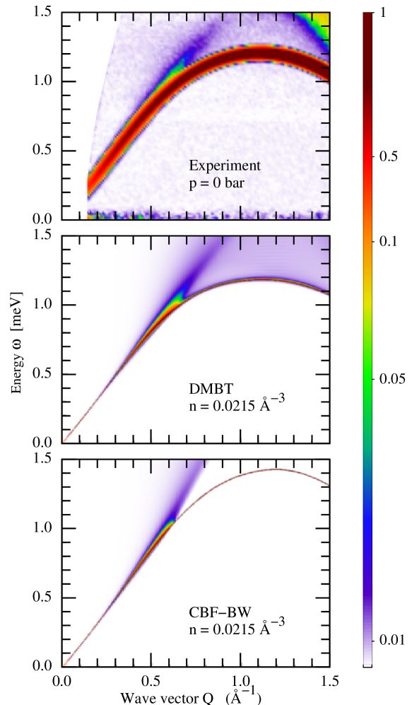
Figure 2: A comparison of theoretical and experimental data for the dynamic structure function $S(k,\omega)$ from experiments skw4lett ; skwpress and two versions of our theory: The middle figure is based on the solution of the integral equation (8), the lowest figure shows the CBF-BW approximation; the only difference to previous work JacksonSkw are more accurate input functions $S(k)$ and $X_{3}({\bf r}_{1},{\bf r}_{2},{\bf r}_{3})$.

In Fig. 2, we compare the experimental dynamic structure function $S(k,\omega)$ (top panel) skw4lett with results from DMBT calculations (middle panel) and CBF-BW calculation JacksonSkw (bottom panel). In the CBF-BW calculation we have, of course, used the best available values for $S(k)$ in the three-phonon vertex (9) and included the irreducible part $\tilde{X}_{3}({\bf q};{\bf k}_{1},{\bf k}_{2})$ as described in Ref. 21. Thus, the numerical values are different from those of Ref. 22 but the physics described is basically the same.

The most significant difference between the CBF-BW approximation and the full solution of the integral equation (8) is the void regime above the phonon-maxon-roton dispersion relation. This is caused by the fact that, in the CBF-BW approximation, excitations decay into Feynman phonons $\varepsilon_{\rm F}(k)$ and not into the physical phonons. Furthermore, CBF-BW overestimates the excitation energies in the maxon region, while DMBT agrees with the experiment.

4 Phonon dispersion

The theoretical phonon dispersion relation is obtained by solving the implicit equation

$$\varepsilon_{0}(k)=\varepsilon_{\rm F}(k)+\Sigma(k,\varepsilon_{0}(k))\,.$$ (10)

At long wave lengths, the phonon dispersion relation is

$$\varepsilon_{0}(k)\approx\hbar ck(1-\gamma k^{2})$$ (11)

where $c$ is the speed of sound and $\gamma$ is the phonon dispersion coefficient. If $\gamma<0$, we speak of anomalous dispersion, long–wavelength phonons are damped.

To obtain the dispersion coefficient $\gamma$ we have fitted both experimental and theoretical data by a polynomial of the form

$$\varepsilon_{0}(k)=\hbar ck\left(1-\gamma k^{2}+\alpha_{3}k^{3}+\alpha_{4}k^{4}\right),$$ (12)

from which the phonon dispersion coefficient was extracted. The polynomial form turned out to be more flexible than the Padé approximation MarisRMP ; PhysRevA.8.1980

$$\varepsilon_{0}(k)=\hbar ck\left(1-\gamma k^{2}\frac{1-k^{2}/Q_{a}^{2}}{1+k^{2}/Q_{b}^{2}}\right)\,.$$ (13)

In particular, the Padé approximation (13) does not contain the term proportional to $k^{3}$ which can be calculated analytically from the asymptotic form of the microscopic two-body interaction. Assuming the typical asymptotic form $V(r)=C_{6}r^{-6}$, one arrives at Pitaevskii1970 ; Feenberg1971

$$\alpha_{3}=\frac{\pi^{2}}{24}\frac{\rho}{mc^{2}}C_{6}\,.$$ (14)

We should note that fitting procedure should not be understood as a rigorous low-$k$ expansion in the sense of a Taylor expansion of the dispersion relation $\epsilon_{0}(k)$ around $k=0$, but rather as a fit to the data in the theoretically and experimentally relevant regime. The fit works well for $k<0.6\,$Å^-1.

To explain the fact that the above fitting procedure should not be considered to be a rigorous Taylor expansion, we must review a little more of the theoretical background. The Feynman spectrum $\varepsilon_{\rm F}(k)$ is derived from a Bogoliubov formula

$$\varepsilon_{\rm F}(k)=\sqrt{t^{2}(k)+2t(k)\tilde{V}_{\rm p-h}(k)}$$ (15)

where $t(k)=\hbar^{2}k^{2}/2m$ is the kinetic energy, and

$$\tilde{V}_{\rm p-h}(k)\equiv\rho\int d^{3}rV_{\rm p-h}(r)e^{\mathrm{i}{\bf k}\cdot{\bf r}}$$ (16)

is the “particle-hole” interaction or, in the language of Aldrich and Pines Aldrich the “pseudopotential”. For what follows we only need the property that, for large distances, $V_{\rm p-h}(r)$ falls off like the bare interaction, i.e. $V_{\rm p-h}(r)\sim C_{6}r^{-6}$ for $r\rightarrow\infty$. Then, $\tilde{V}_{\rm p-h}(k)$ has the expansion

$$\tilde{V}_{\rm p-h}(k)=\tilde{V}_{\rm p-h}(0+)+V_{2}k^{2}+\frac{\pi^{2}}{12}\rho C_{6}k^{3}$$ (17)

where $\tilde{V}_{\rm p-h}(0+)=\rho\int d^{3}rV(r)=mc^{2}$ is related to the speed of sound, and $V_{2}$ is the second moment $V_{2}=-\frac{\rho}{6}\int d^{3}rV_{\rm p-h}(r)r^{2}$. Higher moments do not exist due to the van der Waals tail.

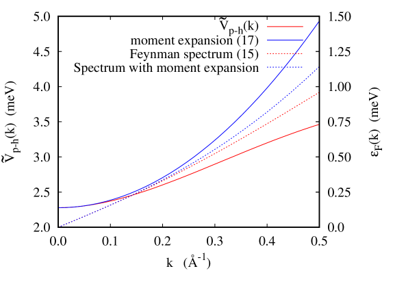
Figure 3: The figure shows the full particle–hole interaction $\tilde{V}_{\rm p-h}(k)$ (solid red line, left scale) and the low-momentum expansion (17) (solid blue line) at a density $\rho=0.0215$Å^-3. Also shown are the Feynman dispersion relations obtained from the Bogoliubov relation (15) for these two cases (red and blue dashed lines, right scale).

Fig. 3 shows the full $\tilde{V}_{\rm p-h}(k)$ the way it is used in the Bogoliubov formula (15) and the expansion (17) as calculated from the potential moments. Evidently, the agreement is very good only in the regime $0\leq k\leq 0.1\,$Å^-1 which is inaccessible to neutron scattering measurements. The figure also shows the Feynman spectrum $\varepsilon_{\rm F}(k)$ as obtained from the full $\tilde{V}_{\rm p-h}(k)$ and from the moment expansion.

Both the DMBT and the CBF-BW results for $\gamma$ agree quite well with the experimental data, whereas the Feynman approximation predicts anomalous dispersion at all densities.

The calculated phase velocities $c=\varepsilon_{0}(k)/\hbar k$ are given in Fig. 4 for densities covering the full range between the saturated vapor pressure and solidification. Also shown are experimental data skw4lett ; skwpress at four pressures corresponding to the same the same density range. Clearly the agreement is excellent. Only a very small shift in density is observed between the theoretical calculations and the experimental results, already discussed in previous publications skw4lett ; skwpress .

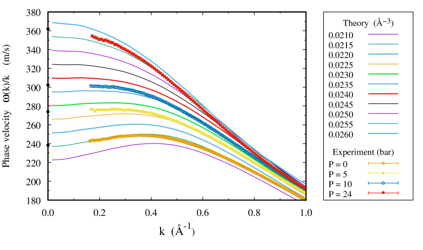
Figure 4: Dispersion relation for several ⁴He densities, comparing experiment (markers for pressures P=0, 5, 10, 24 bar, corresponding to densities $0.0218,0.0230,0.0239$ and $0.0258$Å^-3), and DMBT (lines, for several densities from $0.0210$ to $0.0260$Å^-3 as indicated in the legend). Thick lines indicate theoretical curves for densities close to the experimental values given above. The black dots at $k=0$ indicate the sound velocities determined by ultrasonic techniques Abraham .

The polynomial expression (12) provides an excellent fit of the theoretical curves in the small wave vector range. In practice, fits of the experimental curves were done in the range $0.18<k<\ 0.6\,$Å^-1, the lower bound being determined by the neutron detectors smallest angle. The highest bound was determined as the maximum wave vector where stable fits could be obtained using the form (12). This was also verified for the theoretical curves; for the latter, the fit range could be extended to $k=0$, without affecting significantly the results of the fits, as seen in Fig. 5.

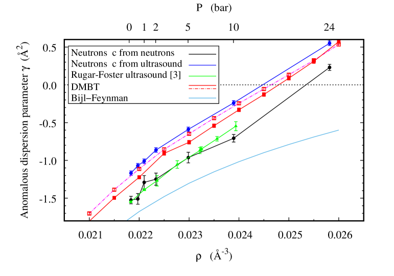
Figure 5: Dispersion coefficient $\gamma$ for several ⁴He densities, comparing neutron scattering experiments (blue and black dots and lines correspond to different data analyses described in the text), ultrasonic measurements Rugar1984 (green triangles) and DMBT results (red lines and solid and open squares). Similar results are found for the different fit ranges $0.0-0.6\,$Å^-1 (dash-dotted red line) and $0.2-0.6\,$Å^-1 (solid red line). We also show the dispersion coefficient coming from the Feynman spectrum (15) (light blue line).

The experimental results have been analyzed using the polynomial expression (12) to determine the dispersion coefficient $\gamma$ for several ⁴He densities. The speed of sound $c$ determined by the fit agrees well with the well know values measured by ultrasonic or thermodynamic techniques Abraham ; CaupinJordi , as can be seen in the extrapolations to $k=0$ in Fig. 5. The agreement is not perfect, however, and this affects the value of the next term in the expansion, the dispersion coefficient $\gamma$. We thus show in Fig. 5 the curves for $\gamma$ determined using either the fitted values of $c$, or the ultrasonic ones.

For completeness, we have also extracted other data from both the calculations and the experiments. Table 1 gives the calculated coefficients $\hbar c$, the speed of sound $c$, the Grüneisen-Constant $u$ and the dispersion coefficient $\gamma$. Static quantities like $c$ and $u$ can also be obtained from Monte Carlo simulations,

$\rho$ (Å^-3) $\hbar c$ (meVÅ) $c$ (m/sec) $u$ $\gamma_{\rm F}$ $\gamma$ $c$  u  $\gamma$ JF-EL DMBT expt./DMC 0.0210  1.466  222.7  2.738  -2.221  -1.804  211.5  3.080  -1.85 0.0215  1.561  237.2  2.628  -1.946  -1.495  227.0  2.944  -1.56 0.0220  1.657  251.7  2.534  -1.710  -1.223  242.6  2.832  -1.29 0.0225  1.752  266.2  2.453  -1.510  -0.906  258.2  2.738  -1.04 0.0230  1.848  280.7  2.384  -1.333  -0.760  274.0  2.657  -0.81 0.0235  1.944  295.3  2.323  -1.182  -0.541  289.9  2.588  -0.60 0.0240  2.040  309.9  2.269  -1.046  -0.330  305.9  2.529 0.0245  2.136  324.6  2.222  -0.925  -0.127  322.1  2.476 0.0250  2.234  339.4  2.179  -0.815  0.087  338.5  2.430 0.0255  2.331  354.2  2.141  -0.713  0.311  355.0  2.388 0.0260  2.429  369.1  2.107  -0.619  0.571  371.7  2.532

Table 1: The table shows in columns 2-6 the calculated values $\hbar c$, the speed of sound $c$, the Grüneisen constant $u$ and the phonon dispersion coefficient $\gamma_{F}$ in Feynman approximation, and as obtained by fitting the dispersion relation by the form (12). Col. 7-9 give the corresponding quantities obtained, as far as possible, from experiments or from Monte Carlo simulations. The experimental results for the dispersion coefficient $\gamma$ have been obtained by interpolating the data of Ref. 3 at the densities in col. 1 by a quadratic polynomial.

Evidently, the agreement between the DMBT results and the experiment is excellent at all densities. The dispersion coefficient $\gamma$ turns positive above $\rho\approx 0.0245$Å^-3, meaning that long–wavelength phonons can propagate freely only at high pressures. The Feynman approximation predicts, on the other hand, a negative dispersion coefficient at all densites.

5 Phonon Mean Free Path

If $\gamma<0$, a phonon of energy/momentum $(\hbar\omega,k)$ can decay into two phonons of lower energy and longer wave length. As a consequence, the self–energy becomes complex on the phonon dispersion relation. The onset of the imaginary part of an excitation of energy and momentum $(\hbar\omega,k)$ is at the critical energy $\hbar\omega_{\rm crit}=2\varepsilon_{0}(k/2)$, where $\varepsilon_{0}(k)$ is the dispersion relation calculated with DMBT, see eq. (10). At a corresponding critical wave number $k_{\rm crit}$ determined by solving $2\varepsilon_{0}(k/2)=\varepsilon_{0}(k)$ for $k$, a phonon can decay into two phonons, parallel to the original phonon but with half the wave number. At this point the imaginary part of the self–energy is bosegas ; eomIII

$$\Sigma(k,\hbar\omega)=-\frac{|\tilde{V}_{3}({\bf k};-{\bf k}/2,-{\bf k}/2)|^{2}k}{16\pi\rho\varepsilon_{0}^{\prime}(k/2)}\sqrt{\frac{2\varepsilon_{0}(k/2)-\hbar\omega}{\varepsilon_{0}^{\prime\prime}(k/2)}}\,.$$ (18)

Phonons with lower wave numbers, $k<k_{\rm crit}$, have more decay channels because the wave vectors of the produced phonons need not be parallel to the original phonon; this angular spread is discussed further below. Phonons with wave numbers $k>k_{\rm crit}$ do not decay into pairs of phonons and have infinite life-time in the DMBT approximation. However, higher-order processes, ı.e. decay into three and more phonons, lead to a long, but finite life-time also for $k>k_{\rm crit}$.

The life time of phonons with $k<k_{\rm crit}$ can be readily calculated from the imaginary part of the self-energy,

$$\tau(k)=\hbar\,\Im m[\Sigma(k,\hbar\varepsilon_{0}(k),k)]^{-1}$$ (19)

The mean free path of a phonon, important for the suggested application of superfluid ⁴He for dark matter detection mentioned above, can be obtained from

$$d(k)=v_{g}(k)\,\tau(k)$$ (20)

where $v_{g}={d\omega(k)\over dk}$ is the group velocity.

Evidently, two things are needed for a reliable theoretical prediction of the phonon life time $\tau(k)$ and of the mean free path $d(k)$. (1) An accurate dispersion coefficient is required for the low-momentum kinematics,

$${\bf k} = {\bf q}+{\bf p}$$ (21)

$$\varepsilon_{0}(k) = \varepsilon_{0}(q)+\varepsilon_{0}(p)$$ (22)

which in particular determines the range of momenta where phonon damping occurs. (2) The three-phonon vertex $V_{3}$ is required for an accurate damping strength. The comparison of the dynamic structure function between experiment and the DMBT result in Fig. 2 shows that DMBT is accurate enough that eqns.(19) and (20) indeed provide a reliable theoretical prediction of phonon life time and mean free path.

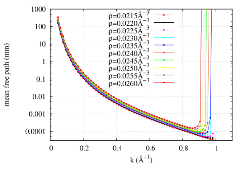
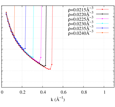
Figure 6: The phonon mean free path $d(k)$ as function of the wave number for different pressures. The left panel shows the result in CBF-BW approximation and the right one shows the improved result obtained with the DMBT method which shows that the phonon mean free path depends strongly on the pressure.

Figs. 6 show our results for the phonon mean free path $d(k)$ in both CBF-BW approximation (left panel) and in DMBT (right panel) for several helium densities $\rho$. The density range is smaller in the latter case, because the dispersion relation is not anomalous anymore for $\rho\gtrsim 0.0245$Å^-3, see the dispersion coefficient $\gamma$ shown in Fig. 5. In the CBF-BW calculation phonons decay by producing Feynman-phonons, which overestimates the anomalous dispersion and which have a negative $\gamma$ for all densities considered here (see Fig.5). Therefore CBF-BW yields a finite mean free path even for $\rho=0.0260$Å^-3. In fact $d(k)$ is almost independent of $\rho$ and thus of the pressure in the CBF-BW approximation, while the much improved DMBT result shows that the range of momenta where phonons can decay strongly depends on $\rho$, hence on the pressure. While CBF-BW predicts a minimal decay length of about $0.1\mu$m for all densities, the DMBT results show that the minimal decay length is $1-10\mu$m around the equilibrium density, and increases significantly with density and pressure, because $\gamma$ crosses zero and becomes positive at high density, Fig.5, until the phonons do not decay anymore for densities higher than $0.0240$Å^-3,

While the DMBT calculation predicts a much smaller range of wave numbers at which phonons are dampened, the values for mean free path $d(k)$ at different densities are almost identical for a given $k$, if there is damping at all. In fact, the $d(k)$ values predicted by CBF-BW and DMBT are essentially the same. The reason is that the lifetime and thus the mean free path are mostly determined by the vertex $V_{3}$, which is the same for CBF-BW and DMBT. The strength of damping does depend on the first derivative of the dispersion which, however, for the small $k$ range relevant here is very similar in all approximations (Feynman, CBF-BW, and DMBT) – only the higher order derivatives, essential for the correct decay kinematics, are sensitive to the approximation.

6 Inelastic currents

Anomalous dispersion is a prerequisite for phonon decay, but the deviation of the dispersion relation from a linear dispersion is, in the wave number regime under consideration here, hardly visible, see Fig. 4. Therefore, a phonon decays into a pair of more or less collinear phonons. The angular distribution of these decay phonons can be obtained from the transport current, which is the second order expectation value of the current operator in the fluctuations $\delta U({\bf r}_{1},\ldots,{\bf r}_{N},t)$

$${\bf j}^{(2)}({\bf r},t) \equiv \frac{1}{4}\Bigl{\langle}{\Psi_{0}}\Bigr{|}\delta U^{*}\,\hat{\bf j}({\bf r})\,\delta U\Bigl{|}{\Psi_{0}}\Bigr{\rangle}$$ (23)

$$= \frac{\hbar N}{8m\mathrm{i}}\int d^{3}r_{2}\ldots d^{3}r_{N}\Psi_{0}^{2}\left[\delta U^{*}(t)\nabla_{1}\delta U(t)-{\rm c.c.}\right]$$

The derivation of workable formulas is somewhat tedious, some essential steps will be presented in the Appendix. A detailed derivation for the case of impurity scattering off the ⁴He surface may be found in Ref. 8, and for the case of impurity and ⁴He scattering in Ref. 7.

The decay of a phonon with wave vector ${\bf k}$ produces two phonons according to the kinematics (21) and (22). We are interested in a measure for the probability that a decay product is ejected in direction ${\bf e}$ (${\bf e}$ is a unit vector with Euler angles $\theta$ and $\varphi$). For this purpose we calculate the rate of inelastic phonon current in direction ${\bf e}$, for which we obtain

$$\frac{d}{dt}j^{(2)}({\bf e})=\frac{1}{mS(k)}\int\frac{d^{3}q}{(2\pi)^{3}\rho}\,q\,\delta({\bf e}-{{\bf q}\over q})\,{\Im m}\,\sigma({\bf k},{\bf q},\omega)$$ (24)

The $\delta({\bf e}-{{\bf q}/q})$ obviously selects only phonons with wave vector ${\bf q}$ parallel to the direction of interest. Here $\sigma({\bf k},{\bf q},\omega)$ is

$$\sigma({\bf k},{\bf q},\omega)=\frac{1}{2}\frac{\left|\tilde{V}({\bf k},{\bf k}-{\bf q},{\bf q})\right|^{2}}{\hbar\omega-\varepsilon_{0}(|{\bf k}-{\bf q}|)-\varepsilon_{0}(q)+\mathrm{i}\eta}$$ (25)

The integration over ${\bf q}$ yields the self energy $\int\frac{d^{3}q}{(2\pi)^{3}\rho}\sigma({\bf q};{\bf k},\omega)=\Sigma({\bf k},\omega)$, see Eq. (8). For the calculation of $\sigma({\bf k},{\bf q},\omega)$, we have replaced the non–local self–energy appearing in Eq. (8) by the dispersion relation (10), this is legitimate in the low momentum regime under consideration.

Fig. 7 shows, at the density $\rho=0.0215$Å^-3, the DMBT prediction for the rate with which a phonon with wave number ${\bf k}$ decays into phonons with direction $\theta$ with respect to ${\bf k}$ (obviously, the rate does not depend on $\varphi$). The figure summarizes both the kinematics and the strength of phonon damping by decay into lower momentum phonons. In agreement with the decay length in the right panel of Fig. 6, the decay rate is highest for phonons with momentum $k$ close to 0.5Å^-1. Fig.7 shows that these higher energy phonons decay into lower energy phonons which lie in a narrow cone (small $\theta$). Phonons with $k=0.2-0.3$Å^-1 decay at a smaller rate (have a larger decay length, see Fig.6), but generate phonons in a larger cone up to angles of $\theta=20^{\circ}$.

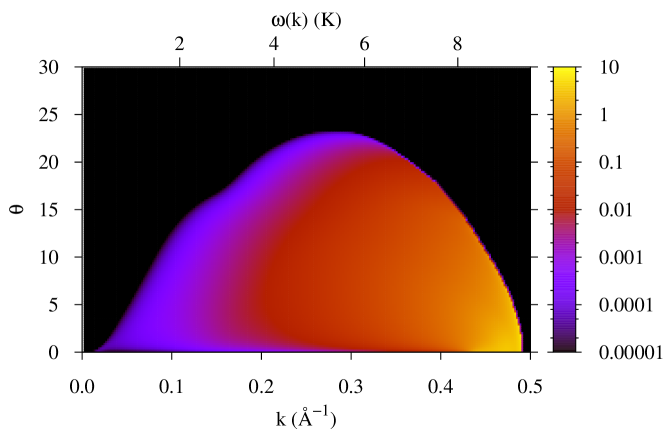
Figure 7: The angular dependence of the phonons produced by the decay of an initial phonon with wave number $k$. $\theta$ is the angle of the decay phonons with respect to the direction of the initial phonon. The density is $\rho=0.0215$Å^-3.

7 Conclusion

The dispersion and damping of low momemtum phonons in superfluid helium-4 is of practical interest for cosmological applications in weakly interacting particle detectors to test hypotheses for dark matter. We presented a comparison of the low momentum dispersion in ⁴He between experimental data and the results from dynamic many-body theory (DMBT) and find excellent agreement. The dispersion obtained with DMBT is a significant improvement over the CBF prediction in the full momentum and energy range of interest. This allows us to make quantitative predictions for the decay of phonons due to the anomalous dispersion without phenomenological or experimental input parameters. The phonon mean free path is similar to CBF-BW results, but the CBF-BW approximation fails to predict the pressure dependence, leading to decay lengths as short as 0.1$\mu$m. This shortcoming is remedied by the DMBT which shows that the minimal decay length is strongly pressure dependent.

Transport current

We present in this appendix the essential steps of the derivation of the transport currents; the details of the derivation are rather similar to the ones for the impurity currents derived in Refs. 8 and 7. We derive the inelastic current at the level of pair fluctuations, i.e. we truncate the expansion (5) at the two-body level. To derive the integral equation (8) one needs to include fluctuations to all orders eomIII ; our result will be plausible enough such that we can avoid these complications.

As in the derivation of the linearized equations of motion for the correlation operator (5), leading to the density–density response function $\chi(k,\omega)$, Eq. (7), it is convenient to apply an weak harmonic perturbation (e.g. induced by a neutron beam)

$$U_{\rm ext}({\bf r};t)=\left[U_{\rm ext}({\bf r})e^{-\mathrm{i}\omega t}+U_{\rm ext}^{*}({\bf r})e^{\mathrm{i}\omega t}\right]e^{\eta t}$$ (26)

As usual, the perturbation is switched on adiabatically with an infinitesimal rate $\eta>0$. After linearization, the positive and negative frequency terms leads to a corresponding response of the correlation operator $\delta U(t)$ split into (complex) positive and negative frequency terms; similarly for the response of one-body, two-body densities, $\delta\rho_{n}$.

Inserting the correlation operator (5) at the two-body level in the transport currents (23) gives (we omit the time dependence for clarity)

$${\bf j}^{(2)}({\bf r})=\frac{\hbar}{4m\mathrm{i}}\left[\delta\rho_{1}^{*}({\bf r}_{1})\nabla_{1}\delta u_{1}({\bf r}_{1})+\int d^{3}r_{2}\delta\rho_{2}^{*}({\bf r}_{1},{\bf r}_{2})\nabla_{1}\delta u_{2}({\bf r}_{1},{\bf r}_{2})\right]\,.$$ (27)

where we have used that we are only interested in the time-averaged currents, since only those are observable by a detector.

While looking very simple, the expression (27) for the current contains both the fluctuations of the correlation and of the densities. In accordance with the derivation of the self energy $\Sigma(k,\hbar\omega)$, summarized in the text, we express $\delta u_{1}$ and $\delta\rho_{2}$ in terms of $\delta\rho_{1}$ and $\delta u_{2}$. It turns out advantageous to introduce $\delta v_{1}({\bf r};t)$ such that

$$\delta\rho_{1}({\bf r}_{1})=\rho\left[S*\delta v_{1}\right]({\bf r}_{1})\,.$$ (28)

where we define the convolution product with the static structure function

$$\left[S*f\right]({\bf r}_{1})=f({\bf r}_{1})+\rho\int d^{3}r_{2}h({\bf r}_{1},{\bf r}_{2})f({\bf r}_{2})\,.$$ (29)

In linear order, we can then write

$$\delta v_{1}({\bf r}) = \delta u_{1}({\bf r})+\delta w_{1}({\bf r})$$

$$\delta w_{1}({\bf r}) = \rho\int d^{3}r_{2}h({\bf r}_{1},{\bf r}_{2})\delta u_{2}({\bf r}_{1},{\bf r}_{2})$$ (30)

$$+\frac{\rho^{2}}{2}\int d^{3}r_{2}d^{3}r_{3}Y({\bf r}_{1};{\bf r}_{2},{\bf r}_{3})\delta u_{2}({\bf r}_{2},{\bf r}_{3})\,,$$

where the $Y({\bf r}_{1};{\bf r}_{2},{\bf r}_{3})$ is the set of those contributions to the three-body distribution function that is non-nodal in the point ${\bf r}_{1}$; details can be found in Ref. eomIII .

In all further manipulations, we use the “convolution approximation” which is the simplest approximation for high-order distribution functions that maintains the exact long-wavelength properties. In convolution approximation, $Y({\bf r}_{1};{\bf r}_{2},{\bf r}_{3})$ is simply

$$Y({\bf r}_{1};{\bf r}_{2},{\bf r}_{3})=h({\bf r}_{1},{\bf r}_{2})h({\bf r}_{1},{\bf r}_{3})\,.$$ (31)

Using Eqs. (30) and (31) and expressing $\delta\rho_{2}({\bf r}_{1},{\bf r}_{2})$ in terms of $\delta\rho_{1}({\bf r})$ and the fluctuation of the pair distribution function $\delta g({\bf r}_{1},{\bf r}_{2})$,

$$\delta\rho_{2}({\bf r}_{1},{\bf r}_{2})=\rho\left[\delta\rho_{1}({\bf r}_{1})+\rho_{1}({\bf r}_{2}\right]\,g({\bf r}_{1},{\bf r}_{2})+\rho_{2}g({\bf r}_{1},{\bf r}_{2})$$

we obtain

$${\bf j}^{(2)}({\bf r};t) = \frac{\hbar}{4m\mathrm{i}}\Biggl{\{}\delta\rho^{*}_{1}({\bf r}_{1})\biggl{[}\nabla_{1}\delta v_{1}({\bf r}_{1})-\rho\int d^{3}r_{2}\delta u_{2}({\bf r}_{1},{\bf r}_{2})\nabla_{1}h({\bf r}_{1},{\bf r}_{2})$$ (32)

$$\qquad-\frac{\rho^{2}}{2}\nabla_{1}\int d^{3}r_{2}d^{3}r_{3}h({\bf r}_{1},{\bf r}_{2})h({\bf r}_{1},{\bf r}_{3})\delta u_{2}({\bf r}_{2},{\bf r}_{3})\biggr{]}$$

$$\qquad+\rho\int d^{3}r_{2}h({\bf r}_{1},{\bf r}_{2})\nabla_{1}\delta u_{2}({\bf r}_{1},{\bf r}_{2})\delta\rho_{1}^{*}({\bf r}_{2})$$

$$\qquad+\rho^{2}\int d^{3}r_{2}\delta g^{*}({\bf r}_{1},{\bf r}_{2})\nabla_{1}\delta u_{2}({\bf r}_{1},{\bf r}_{2})\Biggr{\}}\,.$$

Finally we eliminate $\delta g({\bf r}_{1},{\bf r}_{2})$ using the convolution approximation:

$$\delta g({\bf r}_{1},{\bf r}_{2})=\int d^{3}r_{3}h({\bf r}_{1},{\bf r}_{3})h({\bf r}_{2},{\bf r}_{3})\delta\rho_{1}({\bf r}_{3})+\left[S*\delta u_{2}*S\right]({\bf r}_{1},{\bf r}_{2})\,.$$ (33)

which yields the length expression for the current

$${\bf j}^{(2)}({\bf r}_{1}) = \frac{\hbar}{4m\mathrm{i}}\delta\rho^{*}_{1}({\bf r}_{1})\nabla_{1}\delta v_{1}({\bf r}_{1})$$ (34)

$$+ \frac{\hbar\rho}{4m\mathrm{i}}\int d^{3}r_{2}\nabla_{1}\left[\delta u_{2}*S\right]({\bf r}_{1},{\bf r}_{2})h({\bf r}_{1},{\bf r}_{2})\delta\rho_{1}^{*}({\bf r}_{2})$$ (35)

$$+ \frac{\hbar\rho}{4m\mathrm{i}}\delta\rho^{*}_{1}({\bf r}_{1})\int d^{3}r_{2}\left[S*\delta u_{2}\right]({\bf r}_{1},{\bf r}_{2})\nabla_{1}h({\bf r}_{1},{\bf r}_{2})$$ (36)

$$+ \frac{\hbar}{4m\mathrm{i}}\int d^{3}r_{2}\left[S*\delta u_{2}^{*}*S\right]({\bf r}_{1},{\bf r}_{2})\nabla_{1}\delta u_{2}({\bf r}_{1},{\bf r}_{2})$$ (37)

The first term (34) is the current in Feynman approximation which is the elastic channel. The second and third terms, (35) and (36), are correlations between the density fluctuation $\delta\rho_{1}$ and the pair correlation fluctuation $\delta u_{2}$. We will show below that only the fourth term (37) contains the decay rate of an elementary excitation (in the above derivation given in Feynman approximation).

We now need explicit expressions for the one- and two-body fluctuations. These come from solving the equations of motion, formally given by Eq. (6), in detail given in Refs. 8; 6. We can assume that the perturbation $U_{\rm ext}({\bf r})$ is a plane wave with wave vector ${\bf q}$ which induces a plane wave density fluctuation, propagating with phase velocity given by the dispersion relation, $\omega_{0}(q)=\varepsilon_{0}(q)/\hbar$:

$$\delta\rho({\bf r};t)=\lambda\rho e^{\mathrm{i}({\bf q}\cdot{\bf r}-\omega_{0}(q)t)}e^{\eta t}$$ (38)

where $\lambda\ll 1$ is an arbitrary strength factor.

The two-body correlation fluctuations are then coupled to the density fluctuation according to the equations of motion. Their spatial Fourier transform is given by

$$\tilde{u}_{2}({\bf k}_{1},{\bf k}_{2}) = \frac{\lambda(2\pi)^{3}\delta({\bf q}+{\bf k}_{1}+{\bf k}_{2})}{\varepsilon_{0}(q)-\varepsilon_{0}(k_{1})-\varepsilon_{0}(k_{1})+\mathrm{i}\hbar\eta}\frac{\tilde{V}({\bf q};{\bf k}_{1},{\bf k}_{2})}{\sqrt{S(q)S(k_{1})S(k_{2})}}e^{-\mathrm{i}\omega_{0}(q)t)+\eta t}$$ (39)

We finally use Eq. (38) for $\delta\rho_{1}({\bf r})$ and Eq. (39) for $\delta u_{2}({\bf r}_{1},{\bf r}_{2})$ in the current ${\bf j}^{(2)}({\bf r})$ above. The fourth term (37) which becomes

$$\lambda^{2}\frac{\hbar}{4m}\int\frac{d^{3}k_{1}d^{3}k_{2}}{(2\pi)^{3}\rho}\delta({\bf q}+{\bf k}_{1}+{\bf k}_{2})\,{\bf k}_{1}\,\frac{1}{S(q)}\frac{\left|\tilde{V}({\bf q};{\bf k}_{1},{\bf k}_{2})\right|^{2}}{(\varepsilon_{0}(q)-\varepsilon_{0}(k_{1})-\varepsilon_{0}(k_{2}))^{2}+\hbar^{2}\eta^{2}}\,e^{2\eta t}$$

In the limit of adiabatically switching on the perturbation, $\eta\to 0$, we need to calculate the rate with which the inelastic current is generated, i.e. the time derivative. Using

$$\frac{d}{dt}\frac{e^{2\eta t}}{(\varepsilon_{0}(q)-\varepsilon_{0}(k_{1})-\varepsilon_{0}(k_{2}))^{2}+\hbar^{2}\eta^{2}}\rightarrow\frac{2\pi}{\hbar}\,\delta(\varepsilon_{0}(q)-\varepsilon_{0}(k_{1})-\varepsilon_{0}(k_{2}))$$ (40)

we obtain the rate of the total inelastic current $\frac{d}{dt}{\bf j}^{(2)}$ apart from the arbitrary strength factor $\lambda^{2}$. Selecting only the inelastic phonon current (the decay products) in a specific direction ${\bf e}$ relative to the incoming phonon with wave vector ${\bf q}$, we obtain the rate Eq. (24). Note that the two mixed term contributions to ${\bf j}^{(2)}({\bf r})$, Eqs. (35) and (36), do not have a finite contribution to the rate in the adiabatic limit.

References

- (1) H.J. Maris, Rev. Mod. Phys. 49, 341 (1977)
- (2) H.J. Maris, Phys. Rev. A 8, 1980 (1973). DOI 10.1103/PhysRevA.8.1980. URL https://link.aps.org/doi/10.1103/PhysRevA.8.1980
- (3) D. Rugar, J.S. Foster, Phys. Rev. B 30(5), 2959 (1984)
- (4) R. Sridhar, Physics Reports 146(5), 259 (1987)
- (5) K. Beauvois, J. Dawidowski, B. Fåk, H. Godfrin, E. Krotscheck, H.J. Lauter, J. Ollivier, A. Sultan, Phys. Rev. B 97, 184520 (2018)
- (6) C.E. Campbell, E. Krotscheck, T. Lichtenegger, Phys. Rev. B 91, 184510/1 (2015)
- (7) E. Krotscheck, R. Zillich, J. Chem. Phys. 115(22), 10161 (2001)
- (8) E. Krotscheck, R.E. Zillich, Phys. Rev. B 77(16), 094507 (2008)
- (9) K. Schutz, K.M. Zurek, Phys. Rev. Lett. 117, 121302/1 (2016)
- (10) S. Knapen, T. Lin, K.M. Zurek, Phys. Rev. D 95, 056019 (2017)
- (11) H.J. Maris, G.M. Seidel, D. Stein, Phys. Rev. Lett. 119, 181303 (2017)
- (12) R.K. Romani, D. McKinsey, S. Hertel, A. Biekert, J. Lin, D. Pickney, A. Serafin, V. Velan. Probing sub-GeV dark matter with superfluid helium at HeRALD (2019). URL https://absuploads.aps.org/presentation.cfm?pid=15217
- (13) J. Tiffenberg, M. Sofo-Haro, A. Drlica-Wagner, R. Essig, Y. Guardincerri, S. Holland, T. Volansky, T.T. Yu, Phys. Rev. Lett. 119, 131802 (2017). DOI 10.1103/PhysRevLett.119.131802. URL https://link.aps.org/doi/10.1103/PhysRevLett.119.131802
- (14) R.A. Aziz, F.R.W. McCourt, C.C.K. Wong, Molec. Phys. 61, 1487 (1987)
- (15) J. Boronat, in Microscopic Approaches to Quantum Liquids in Confined Geometries, ed. by E. Krotscheck, J. Navarro (World Scientific, Singapore, 2002), pp. 21–90
- (16) R.A. Cowley, A.D.B. Woods, Can. J. Phys. 49, 177 (1971)
- (17) E.C. Svensson, V.F. Sears, A.D.B. Woods, P. Martel, Phys. Rev. B 21, 3638 (1980)
- (18) H.N. Robkoff, R.B. Hallock, Phys. Rev. B 24, 159 (1981)
- (19) M.R. Gibbs, K.H. Andersen, W.G. Stirling, H. Schober, J. Phys. Condens. Matter 11, 603 (1999)
- (20) C.C. Chang, C.E. Campbell, Phys. Rev. B 13(9), 3779 (1976)
- (21) C.E. Campbell, E. Krotscheck, Phys. Rev. B 80, 174501/1 (2009)
- (22) H.W. Jackson, Phys. Rev. A 8, 1529 (1973)
- (23) K. Beauvois, C.E. Campbell, B. Fåk, H. Godfrin, E. Krotscheck, H.J. Lauter, T. Lichtenegger, J. Ollivier, A. Sultan, Phys. Rev. B 94, 024504 (2016)
- (24) M.P. Kemoklidze, L.P. Pitaevskii, Zh. Exsp. Teor. Fiz. 59, 2187 (1970). [Sov. Phys. JETP 32, 1183 (1971)]
- (25) E. Feenberg, Phys. Rev. Lett. 26, 301 (1971)
- (26) C.H. Aldrich, D. Pines, J. Low Temp. Phys. 25, 677 (1976)
- (27) B.M. Abraham, Y. Eckstein, J.B. Ketterson, M. Kuchnir, P.R. Roach, Phys. Rev. A 1(2), 250 (1970). DOI 10.1103/PhysRevA.1.250. URL https://link.aps.org/doi/10.1103/PhysRevA.1.250
- (28) F. Caupin, J. Boronat, K.H. Andersen, J. Low Temp. Phys. 152, 108 (2008)
- (29) V. Apaja, J. Halinen, V. Halonen, E. Krotscheck, M. Saarela, Phys. Rev. B 55, 12925 (1997)