Efficient Low-Rank Semidefinite Programming with Robust Loss Functions

Abstract

In real-world applications, it is important for machine learning algorithms to be robust against data outliers or corruptions. In this paper, we focus on improving the robustness of a large class of learning algorithms that are formulated as low-rank semi-definite programming (SDP) problems. Traditional formulations use the square loss, which is notorious for being sensitive to outliers. We propose to replace this with more robust noise models, including the $\ell_{1}$-loss and other nonconvex losses. However, the resultant optimization problem becomes difficult as the objective is no longer convex or smooth. To alleviate this problem, we design an efficient algorithm based on majorization-minimization. The crux is on constructing a good optimization surrogate, and we show that this surrogate can be efficiently obtained by the alternating direction method of multipliers (ADMM). By properly monitoring ADMM’s convergence, the proposed algorithm is empirically efficient and also theoretically guaranteed to converge to a critical point. Extensive experiments are performed on four machine learning applications using both synthetic and real-world data sets. Results show that the proposed algorithm is not only fast but also has better performance than the state-of-the-arts.

1 Introduction

Many machine learning problems involve the search for matrix-valued solutions. The corresponding optimization problems are often formulated as linear semidefinite programs (SDP) [1, 2, 3, 4] of the form:

$$\min\nolimits_{Z\in\mathbb{S}_{+}}\text{tr}(ZA)\quad\text{s.t.}\;\text{tr}(ZQ_{\tau})=t_{\tau},\;\forall\tau=1,\dots,m,$$ (1)

in which the objective is linear and the target matrix $Z\in{\mathbb{R}}^{n\times n}$ is positive semi-definite (PSD). Here, ${\mathbb{S}}_{+}$ is the cone of PSD matrices, $Q_{\tau}$ and $A$ are some matrices and $t_{\tau}$ is a scalar. Prominent examples include matrix completion [5, 6, 7, 8, 9], ensemble learning [10], clustering [11, 12], sparse PCA [13, 14, 15], maximum variance unfolding (MVU) [16, 17], and non-parametric kernel learning (NPKL) [18, 19]. The instantiations of $Q_{\tau},t_{\tau}$ and $A$ are application-dependent (with details in Section 5). For example, in matrix completion, $Q_{\tau}$ is constructed from the positions of observed entries, $t_{\tau}$ is the corresponding observed value, and $A$ is the identity matrix. In NPKL, $Q_{\tau}$ is constructed from sample indices in the must-link/cannot-link constraint, $t_{\tau}$ indicates whether it is a must-link or cannot-link, and $A$ is a Laplacian matrix for the data manifold.

A standard SDP solver is the interior-point method (IPM) [1]. In each iteration, a sub-problem based on the Lagrangian and log-det barrier function has to be solved numerically, and each such sub-problem iteration takes ${\mathcal{O}}(n^{3})$ time. To reduce the computational cost, Yang et al. [20] introduced an efficient Newton-based algorithm SDPNAL+ to solve the augmented Lagrangian of (1). While ${\mathcal{O}}(n^{3})$ time is still required in each iteration of the sub-problem, the total number of iterations can be much smaller, and enables SDPNAL+ to be faster than IPM.

An alternative approach is to completely avoid enforcing the variate to be PSD. Instead, $Z$ is replaced by a low-rank decomposition $XX{{}^{\top}}$, where $X\in{\mathbb{R}}^{n\times r}$ and $\text{rank}(Z)\leq r$ [21, 22, 11, 23, 4]. Many learning problems, such as matrix completion, MVU and NPKL, also prefer a low-rank $Z$. Problem (1) is then transformed to the nonlinear optimization problem:

$$\!\!\!\min\nolimits_{X}\text{tr}(XX{{}^{\top}}A)\;\text{s.t.}\;\text{tr}(XX{{}^{\top}}Q_{\tau})=t_{\tau},\;\forall\tau=1,\dots,m.$$ (2)

It can be shown theoretically that the factorized problem is equivalent to the original problem when the rank of the solution is deficient [23, 22, 24, 25, 26, 27]. Burer and Monteiro [21] introduced SDPLR, which uses the augmented Lagrangian method together with limited memory BFGS to solve (2). Due to the loss of convexity, more inner and outer loop iterations may be needed.

To avoid handling the $m$ difficult constraints ($\text{tr}(XX{{}^{\top}}Q_{\tau})$ $=$ $t_{\tau}$) in (2), a common trick is to allow them to be slightly violated [28] This leads to the optimization problem:

$$\min_{X}\sum\nolimits_{\tau=1}^{m}\frac{1}{2}(\text{tr}(X{{}^{\top}}Q_{\tau}X)-t_{\tau})^{2}+\frac{\gamma}{2}\text{tr}(X{{}^{\top}}AX),$$ (3)

where the first term measures constraint violations, and $\gamma$ is a hyper-parameter controlling the corresponding penalty. To prevent over-fitting, we further add the regularizer $\|X\|_{F}^{2}$ to (3), leading to:

$$\!\!\!\!\!\min_{X}\!\sum\nolimits_{\tau=1}^{m}\!\frac{1}{2}(\text{tr}(X^{\top}\!Q_{\tau}X)\!-\!t_{\tau})^{2}\!+\!\frac{\gamma}{2}\text{tr}(X^{\top}\!\!AX)\!+\!\frac{\lambda}{2}\|X\|_{F}^{2},\!\!$$ (4)

where $\lambda>0$ is a tradeoff parameter. This regularizer has also been popularly used in matrix factorization applications [29, 30, 31, 32]. One then only needs to solve the smooth unconstrained optimization problem (4) w.r.t. $X$. Gradient descent [24, 25, 33] has been developed as the state-of-the-art solver for this type of problems. It has convergence guarantees with linear/sub-linear convergence rates for certain low-rank formulations [24, 34].

Recall that the square loss is used in (3) and (4) to measure constraint violations. It is well-known that the square loss is sensitive to outliers [35, 36, 37, 30, 32]. This can be problematic as, for example, in MVU, the samples can be corrupted [38]; in kernel learning, the similarity constraints may come from spammers [39]; in matrix completion, there can be attacks in the observed entries [40, 41]. These corruptions and noise can significantly deteriorate the performance [39, 32]. To make the models more robust, a common approach is to replace the square loss by more robust noise models. These include the $\ell_{1}$-loss [35, 42] and, more recently, concave losses such as the minimax concave penalty (MCP) [43] and log-sum penalty (LSP) [44]. These concave loss functions are similar in shape to Tukey’s biweight function in robust statistics [35], which flattens more for larger values. Recently, they have also been successfully used in matrix factorization [36, 45, 37, 30, 46, 32, 47, 41]. However, so far they have not been used in SDPs.

Motivated by the needs for both optimization efficiency and robustness in learning the matrix variate, we propose in this paper the use of robust loss functions with the matrix factorization in (4). However, the resulting optimization problem is neither convex (due to factorization) nor smooth (due to the robust loss). Hence, none of the above-mentioned solvers can be used. To handle this difficult problem, we propose a new optimization algorithm based on Majorization-Minimization (MM) [48, 49]. The crux of MM is on constructing a good surrogate that is easier to optimize. We show that this surrogate can be efficiently optimized by the alternating direction method of multipliers (ADMM) [50, 51]. While MM only guarantees convergence to limit points, we show that the proposed algorithm ensures convergence to a critical point even when the ADMM is only solved inexactly. Efficiency and robustness of the proposed algorithm are demonstrated on five machine learning applications, namely, PSD matrix completion, nonparametric kernel learning, maximum variance unfolding, sparse PCA, and symmetric non-negative matrix factorization. Results show that it is not only faster, but also has better performance over the state-of-the-arts.

A preliminary version of this paper has been published in the IJCAI-2019 conference [52]. Compared with the conference version, the major changes here are:

• In [52], we assumed that the optimization of the convex surrogate is solved exactly. Here, we allow the subproblem to be solved only inexactly, making the whole algorithm more efficient in practice (Section 3.1.2). Besides, we show that when the inexactness is properly controlled, convergence to critical points is still theoretically guaranteed (Section 3.2).

• To further promote robustness, we consider using a nonconvex loss (Section 4) to replace the $\ell_{1}$-loss used in the conference version. We show that the proposed algorithm can still be applied with some modifications, and convergence is also guaranteed.

• Two more applications namely, PSD matrix completion (Section 5.1) and symmetric nonnegative matrix factorization (Section 5.5), are presented.

• Extensive experiments with more applications, baseline algorithms, convergence studies, and ablation study are performed in Section 6.

Notations. We use uppercase letters for matrices, and lowercase letters for scalars. The transpose of a vector or matrix is denoted by the superscript $(\cdot)^{\top}$. The identity matrix is denoted $I$. For a matrix $A=[a_{ij}]$, $\left\|A\right\|_{F}=(\sum\nolimits_{ij}a_{ij}^{2})^{1/2}$ is its Frobenius norm; $\|A\|_{*}=\sum\nolimits_{i}\sigma_{i}(A)$ is its nuclear norm, where $\sigma_{i}(A)$ is the $i$th singular value of $A$; and $\text{tr}(A)$ is its trace (when the matrix is square). A matrix is positive semi-definite (PSD) if its eigenvalues are non-negative. Besides, $\odot$ denotes the element-wise product between two matrices: $[A\odot B]_{ij}=A_{ij}B_{ij}$; and $\lvert\mathcal{S}\rvert$ is the size of a set $\mathcal{S}$.

2 Related Works

2.1 Majorization-Minimization (MM)

Majorization-minimization (MM) [48, 49] is a general technique to make difficult optimization problems easier. Consider a function $f(X)$, which is hard to optimize. Let the iterate at the $k$th MM iteration be $X_{k}$. The next iterate is generated as

$$X_{k+1}=X_{k}+\arg\min\nolimits_{{\tilde{X}}}h_{k}({\tilde{X}};X_{k}),$$ (5)

where $h_{k}$ is a surrogate that is being optimized instead of $f$. A good surrogate should have the following properties [48]:

• $f({\tilde{X}}+X_{k})\leq h_{k}({\tilde{X}};X_{k})$ for any $\tilde{X}$;

• $0\in\arg\min_{\tilde{X}}(h_{k}({\tilde{X}};X_{k})-f({\tilde{X}}+X_{k}))$ and $f(X_{k})=h_{k}(\bm{0};X_{k})$; and

• $h_{k}$ is convex on $\tilde{X}$.

Condition (P3) allows the minimization of $h_{k}$ in (6) to be easily solved. Moreover, from (P1) and (P2), we have

$$f(X_{k+1})\leq\min\nolimits_{\tilde{X}}h(\tilde{X};X_{k})\leq h(\bm{0};X_{k})=f(X_{k}).$$ (6)

Thus, the objectives obtained in successive iterations are non-increasing. However, MM does not guarantee convergence of the sequence $\{X_{k}\}$ [49, 48, 53, 32].

2.2 Alternating Direction Method of Multipliers (ADMM)

Recently, the alternating direction method of multipliers (ADMM) [50, 51] has been popularly used in machine learning and data mining. Consider optimization problems of the form

$$\min\nolimits_{X,Y}\;\phi(X)+\psi(Y)\;:\;AX+By=c,$$ (7)

where $\phi,\psi$ are convex functions, and $A,B$ (resp. $c$) are constant matrices (resp. vector). ADMM considers the augmented Lagrangian $\mathcal{L}(X,Y,\nu)=\phi(X)+\psi(Y)+\nu^{\top}(AX+By-c)+\frac{\rho}{2}\|AX+By-c\|_{2}^{2},$ where $\nu$ is the dual variable, and $\rho>0$ is a penalty parameter. At the $t$th iteration, the values of $X$ and $Y$ (denoted $X_{t}$ and $Y_{t}$) are updated by minimizing $\mathcal{L}(X,Y,\nu_{t})$ w.r.t. $X$ and $Y$ in an alternating manner:

$$X_{t+1}= \arg\min\nolimits_{X}\mathcal{L}(X,Y_{t},\nu_{t}),$$ (8)

$$Y_{t+1}= \arg\min\nolimits_{Y}\mathcal{L}(X_{t+1},Y,\nu_{t}).$$ (9)

Then, $\nu$ is updated as $\nu_{t+1}=\nu_{t}+\rho(AX_{t+1}+BY_{t+1}-c)$.

2.3 Robust Matrix Factorization (RMF)

In matrix factorization (MF), the data matrix $O\in{\mathbb{R}}^{m\times n}$ is approximated by $UV^{\top}$, where $U\in{\mathbb{R}}^{m\times r}$, $V\in{\mathbb{R}}^{n\times r}$ and $r\ll\min(m,n)$ is the rank. In general, some entries of $O$ may be missing (as in applications such as structure from motion [54] and recommender systems [29]). The MF problem is thus formulated as:

$$\min_{U,V}\frac{1}{2}\|\Omega\odot(O-UV^{\top})\|_{F}^{2}+\frac{\lambda}{2}(\|U\|_{F}^{2}+\|V\|_{F}^{2}),$$ (10)

where $\Omega\in\{0,1\}^{m\times n}$ contain indices to the observed entries in $O$ (with $\Omega_{ij}=1$ if $O_{ij}$ is observed, and 0 otherwise), and $\lambda\geq 0$ is a regularization parameter. The square loss in (10) is sensitive to outliers. In [36], it is replaced by the $\ell_{1}$-loss, leading to robust matrix factorization (RMF):

$$\min_{U,V}\|\Omega\odot(O-UV^{\top})\|_{1}+\frac{\lambda}{2}(\|U\|_{F}^{2}+\|V\|_{F}^{2}).$$ (11)

In recent years, many RMF solvers have been developed, e.g., [45, 55, 32, 30]. However, as the objective in (11) is neither convex nor smooth, these solvers lack scalability, robustness and/or convergence guarantees. Recently, the RMF-MM algorithm [32] solves (11) using MM. Let the $k$th iterate be $(U_{k},V_{k})$. RMF-MM tries to find increments $(\tilde{U},\tilde{V})$ that should be added to $(U_{k},V_{k})$ in order to obtain the target $(U,V)$, i.e., $U=U_{k}+\tilde{U}$ and $V=V_{k}+\tilde{V}$. Substituting into (11), the objective can be rewritten as

$$F^{k}(\tilde{U},\tilde{V})\equiv \|\Omega\odot(O\!-\!(U_{k}+\tilde{U})(V_{k}+\tilde{V})^{\top})\|_{1}$$

$$+\frac{\lambda}{2}\|U_{k}+\tilde{U}\|_{F}^{2}+\frac{\lambda}{2}\|V_{k}+\tilde{V}\|_{F}^{2}.$$

The following Proposition constructs a surrogate $H^{k}$ satisfying properties (P1)-(P3) in Section 2.1 for being a good MM surrogate. Unlike $F^{k}$, $H^{k}$ is jointly convex in $(\tilde{U},\tilde{V})$.

Proposition 1 ([32]).

Let $\text{nnz}(\Omega_{(i,:)})$ (resp. $\text{nnz}(\Omega_{(:,j)})$) be the number of nonzero elements in the $i$th row (resp. $j$th column) of $\Omega$, $\Lambda^{r}=\text{Diag}(\sqrt{\smash[b]{\text{nnz}(\Omega_{(1,:)})}},\dots,\sqrt{\smash[b]{\text{nnz}(\Omega_{(m,:)})}})$, and $\Lambda^{c}=\text{Diag}(\sqrt{\smash[b]{\text{nnz}(\Omega_{(:,1)})}},\dots,\sqrt{\smash[b]{\text{nnz}(\Omega_{(:,n)})}})$. Then, $F^{k}(\tilde{U},\tilde{V})\leq H^{k}(\tilde{U},\tilde{V})$, where

$$\!\!\!\!H^{k}(\tilde{U},\tilde{V}) \!\equiv\!\|\Omega\!\odot\!(O\!-\!U_{k}V_{k}^{\top}\!-\!\tilde{U}V_{k}^{\top}\!-\!U_{k}\tilde{V}^{\top})\|_{1}\!+\!\frac{1}{2}\|\Lambda^{r}\tilde{U}\|_{F}^{2}$$

$$+ \frac{\lambda}{2}\|U_{k}+\tilde{U}\|_{F}^{2}+\frac{\lambda}{2}\|V_{k}+\tilde{V}\|_{F}^{2}+\frac{1}{2}\|\Lambda^{c}\tilde{V}\|_{F}^{2}.$$ (12)

Equality holds iff $(\tilde{U},\tilde{V})=(0,0)$.

Because of the coupling of $\tilde{U},V_{k}$ (resp. $U_{k},\tilde{V}$) in $\tilde{U}V_{k}^{\top}$ (resp. $U_{k}\tilde{V}^{\top}$) in (12), $H^{k}$ is still difficult to optimize. Thus, RMF-MM uses ADMM to optimize (12). RMF-MM is guaranteed to generate critical points of (11).

3 SDP Learning with $\ell_{1}$-Loss

Here, we replace the square loss in (4) by the more robust $\ell_{1}$-loss. This leads to the following robust version of (4):

$$\min_{X}R(X)\equiv\sum\nolimits_{\tau=1}^{m} \lvert\text{tr}(X{{}^{\top}}Q_{\tau}X)-t_{\tau}\rvert$$

$$+\frac{\gamma}{2}\text{tr}(X^{\top}AX)+\frac{\lambda}{2}\|X\|_{F}^{2}.$$ (13)

With the $\ell_{1}$-loss, the objective in (13) is neither convex nor smooth. Hence, existing algorithms for solving (4) (such as L-BFGS [21], gradient descent [24, 25], and coordinate descent [56]) can no longer be used.

3.1 Optimization Algorithm

Recall from Section 2.1 that MM is a general technique to make difficult optimization problems easier to optimize. Recently, MM has also been used successfully in the RMF solvers of RMF-MM [32] and RMFNL [41]. In this Section, we design an efficient solver for (13) based on MM. While RMF-MM and RMFNL construct the surrogate by first factorizing the target matrix $Z$ as $XY^{\top}$ and then bounding $X$ and $Y$ separately, our construction of the surrogate for (13) is significantly different.

3.1.1 Constructing a Convex Surrogate

Let $X_{k}$ be the iterate at the $k$th MM iteration. Recall from (5) that the next iterate is constructed as $X_{k}+\tilde{X}$ for some $\tilde{X}\in{\mathbb{R}}^{n\times r}$. The following Lemma bounds $R$ for any $\tilde{X}$, where $R$ is the objective defined in (13).

Lemma 1.

Let $C=A+\frac{\lambda}{\gamma}I$. For any $\tilde{X}\in{\mathbb{R}}^{n\times r}$,

$$R(X_{k}+{\tilde{X}})\leq\sum\nolimits_{\tau=1}^{m}\lvert\text{tr}(2{\tilde{X}}{{}^{\top}}Q_{\tau}X_{k}+X_{k}^{\top}Q_{\tau}X_{k})-t_{\tau}\rvert$$

$$\!+\!\sum\nolimits_{\tau=1}^{m}\lvert\text{tr}({\tilde{X}}{{}^{\top}}Q_{\tau}{\tilde{X}})\rvert\!+\!\frac{\gamma}{2}\text{tr}({\tilde{X}}^{{}^{\top}}C{\tilde{X}}+(X_{k}+2{\tilde{X}})^{\top}CX_{k}).$$

As $|\text{tr}(\tilde{X}^{\top}Q_{\tau}{\tilde{X}})|$ is convex only when $Q_{\tau}\in{\mathbb{S}}_{+}$ [3], the upper bound above is not convex in general. The following provides a looser bound on $|\text{tr}(\tilde{X}^{\top}Q_{\tau}{\tilde{X}})|$ which is convex w.r.t. ${\tilde{X}}$. We first introduce some notations. Given a symmetric square matrix $M$, let its eigenvalues be $\gamma_{i}$’s and the corresponding eigenvectors be $v_{i}$’s. Let $M_{+}=\sum\nolimits_{i}\max(\gamma_{i},0)v_{i}v_{i}{{}^{\top}}$ be the matrix constructed by using only the positive eigenvalues, and similarly $M_{-}=\sum\nolimits_{i}\min(\gamma_{i},0)v_{i}v_{i}{{}^{\top}}$ is constructed from only the negative eigenvalues. Obviously, $M=M_{+}+M_{-}$.

Lemma 2.

$|\text{tr}({\tilde{X}}{{}^{\top}}Q_{\tau}{\tilde{X}})|\leq\text{tr}({\tilde{X}}{{}^{\top}}\bar{Q}_{\tau}{\tilde{X}})$, where $\bar{Q}_{\tau}=\frac{1}{2}(Q_{\tau}+Q_{\tau}^{\top})_{+}-\frac{1}{2}(Q_{\tau}+Q_{\tau}^{\top})_{-}$ is PSD.

Combining Lemmas 1 and 2, a surrogate $H_{k}$ is constructed as follows.

Proposition 2.

$R({\tilde{X}}+X_{k})\leq H_{k}({\tilde{X}};X_{k})$, where

$$H_{k}({\tilde{X}};X_{k})\!\!\!\! \equiv \!\!\!\!\text{tr}({\tilde{X}}{{}^{\top}}(B{\tilde{X}}+\gamma CX_{k}))$$ (14)

$$\!\!\!+ \!\!\!\!\!\!2\sum\nolimits_{\tau=1}^{m}\lvert\text{tr}({\tilde{X}}{{}^{\top}}Q_{\tau}X_{k})+(b_{k})_{\tau}\rvert+c_{k},$$

with $B=\sum\nolimits_{\tau=1}^{m}\bar{Q}_{\tau}+\frac{1}{2}(\lambda I+\gamma A_{+})$, $C=A+\frac{\lambda}{\gamma}I$, $(b_{k})_{\tau}=\frac{1}{2}(\text{tr}(X_{k}{{}^{\top}}Q_{\tau}X_{k})-t_{\tau})$, $c_{k}=\frac{\gamma}{2}\text{tr}(X_{k}{{}^{\top}}(A+\frac{\lambda}{\gamma}I)X_{k})$. Equality holds iff $\tilde{X}=\mathbf{0}$.

It is easy to see that $H_{k}({\tilde{X}};X)$ is convex w.r.t. ${\tilde{X}}$ and $R(X_{k})=H_{k}(\bm{0};X_{k})$. Besides, from Proposition 2, we also have $R({\tilde{X}}+X_{k})\leq H_{k}({\tilde{X}};X_{k})$ for any $\tilde{X}$, and $\mathbf{0}=\arg\min_{\tilde{X}}(H_{k}({\tilde{X}};X_{k})-R({\tilde{X}}+X_{k}))$. Thus, $H_{k}$ satisfies the three desired properties for a MM surrogate in Section 2.1.

TABLE I: Comparison of the proposed SDP-RL algorithm with existing algorithms on matrix completion problems (details are in Section 5.1). The last row shows SDP-RL on sparse data, where “nnz” is the number of nonzero elements. For algorithms with subproblems, $T$ is the number of iterations to solve the subproblem.

		model		complexity
		factorized	loss	space	time (per-iteration)
FW [5]		$\times$	square loss	${\mathcal{O}}(n^{2})$	${\mathcal{O}}(n^{2})$
L-BFGS [28]		$\surd$	square loss	${\mathcal{O}}(nr)$	${\mathcal{O}}(nr^{2})$
nmAPG [57]		$\surd$	square loss	${\mathcal{O}}(nr)$	${\mathcal{O}}(nr^{2})$
ADMM($\ell_{1}$) [50]		$\times$	$\ell_{1}$ loss	${\mathcal{O}}(n^{2})$	${\mathcal{O}}(n^{2}rT)$
SDPLR [21]		$\times$	$\ell_{1}$ loss	${\mathcal{O}}(nr)$	${\mathcal{O}}(n^{2}rT)$
SDPNAL+ [20]		$\times$	$\ell_{1}$ loss	${\mathcal{O}}(n^{2})$	${\mathcal{O}}(n^{3}T)$
SDP-RL	dense data	$\surd$	$\ell_{1}$ loss or	${\mathcal{O}}(n^{2})$	${\mathcal{O}}(n^{2}rT)$
	sparse data		nonconvex loss	${\mathcal{O}}(\text{nnz}(\Omega)+nr)$	${\mathcal{O}}((\text{nnz}(\Omega)r+nr^{2})T)$

3.1.2 Solving the Surrogate Inexactly by ADMM

From (5), $X_{k}$ is updated at the $k$th MM iteration as $X_{k+1}=X_{k}+{\tilde{X}}^{*}$, where

$${\tilde{X}}^{*}=\arg\min\nolimits_{{\tilde{X}}}H_{k}({\tilde{X}};X_{k}).$$ (15)

First, (15) can be easily rewritten as

$$\min\nolimits_{{\tilde{X}},\{e_{\tau}\}} \!\!\!\!\!\text{tr}({\tilde{X}}{{}^{\top}}(B{\tilde{X}}+\gamma CX_{k}))+2\sum\nolimits_{\tau=1}^{m}\lvert e_{\tau}\rvert+c_{k}$$

s.t. $$\!\!\!\!\!e_{\tau}=\text{tr}({\tilde{X}}{{}^{\top}}Q_{\tau}X_{k})+(b_{k})_{\tau},\;\tau=1,\dots,m.$$

As in Section 2.2, let $\tilde{\nu}_{\tau}$ be the dual variable associated with the $\tau$th constraint in (3.1.2). The dual of (3.1.2) is given by the following Proposition.

Proposition 3.

The dual problem of (3.1.2) is

$$\max\nolimits_{\{\tilde{\nu}_{\tau}\}\in\mathcal{C}}\mathcal{D}_{k}(\{\tilde{\nu}_{\tau}\}),$$ (17)

where $\mathcal{D}_{k}(\{\tilde{\nu}_{\tau}\})$ $=$ $c_{k}\!+\!$ $\frac{\gamma}{2}$ $\sum\nolimits_{\tau=1}^{m}$ $\tilde{\nu}_{\tau}(\text{tr}((CX_{k})^{\top}B^{-1}$ $Q_{\tau}X_{k})$ $\!-\!$ $\frac{2}{\gamma}(b_{k})_{\tau})$ $\!-\!$ $\frac{1}{4}$ $\sum\nolimits_{\tau_{1}=1}^{m}$ $\sum\nolimits_{\tau_{2}=1}^{m}$ $\tilde{\nu}_{\tau_{1}}\!$ $\tilde{\nu}_{\tau_{2}}\!$ $(\text{tr}((Q_{\tau_{1}}X_{k})^{\top}\!\!B^{-1}$ $(Q_{\tau_{2}}X_{k}))$ $\!-\!$ $\frac{\gamma^{2}}{4}$ $\text{tr}((CX_{k})^{\top}$ $\!\!B^{-1}$ $(CX_{k}))$ and $\mathcal{C}=\cup_{\tau=1}^{m}\{\tilde{\nu}_{\tau}\,|\,|\tilde{\nu}_{\tau}|\leq 2\}$.

By using the Slater condition [3], the following Lemma shows that strong duality for (3.1.2) and (17) holds.

Lemma 3.

Strong duality for (3.1.2) and (17) holds.

In the following, we again use ADMM to solve (3.1.2). At the $k$th ADMM iteration, it can be easily shown that the updates in (8) and (9) have the following closed-form solutions:

$${\tilde{X}}_{t+1} ={\tilde{X}}_{t}-\tilde{B}_{k}^{-1}(2B{\tilde{X}}_{t}+\tilde{C}_{k}X_{k}),$$ (18)

$$(e_{\tau})_{t+1} =\max(0,\tilde{e}^{-}_{\tau})+\min(0,\tilde{e}^{+}_{\tau}),$$ (19)

where $\tilde{B}_{k}$ $=$ $2B+\rho\sum\nolimits_{\tau=1}^{m}Q_{\tau}X_{k}X_{k}^{\top}Q_{\tau}^{\top}$, $\tilde{C}_{k}$ $=$ $\gamma C$ $+$ $\sum\nolimits_{\tau=1}^{m}$ $(\rho(\text{tr}({\tilde{X}}_{t}{{}^{\top}}Q_{\tau}X_{k})-e_{\tau}+(b_{k})_{\tau}){-}\tilde{\nu}_{\tau})Q_{\tau}$, and $\tilde{e}^{\pm}_{\tau}$ $=$ $\text{tr}({\tilde{X}}_{t+1}^{{{}^{\top}}}Q_{\tau}X_{k})+(b_{k})_{\tau}+\frac{\tilde{\nu}_{\tau}\pm 2}{2\rho}$. Each of the ADMM dual variables $\{\tilde{\nu}_{\tau}\}_{\tau=1,\dots,m}$ is then updated as

$$\!\!\!(\tilde{\nu}_{\tau})_{t+1} \!=\!(\tilde{\nu}_{\tau})_{t}\!+\!\rho\big{(}(e_{\tau})_{t+1}\!-\!\text{tr}({\tilde{X}}_{t+1}{{}^{\top}}Q_{\tau}X_{k})\!+\!(b_{k})_{\tau}\big{)}.$$ (20)

Because of strong duality (Lemma 3), the duality gap is zero at optimality. Recall that (15) and (3.1.2) have the same objective value, one can thus use the duality gap

$$\delta_{k}({\tilde{X}}_{t},\{(\tilde{\nu}_{\tau})_{t}\})=H_{k}({\tilde{X}}_{t};X_{k})-\mathcal{D}_{k}(\{(\tilde{\nu}_{\tau})_{t}\}),$$ (21)

at the $t$th ADMM iteration to monitor convergence. In other words, the ADMM iterations can be stopped and an approximate solution to (15) is found when $\delta_{k}({\tilde{X}}_{t},\{(\tilde{\nu}_{\tau})_{t}\})$ is smaller than a pre-defined threshold $\epsilon_{k}$. The whole procedure for approximately solving subproblem (15) is shown in Algorithm 1.

Algorithm 1 Solving subproblem (15) by ADMM.

0:  pre-defined tolerance $\epsilon_{k}$;

1:  Initialization: $t=1,\tilde{X}_{1}=0$;

2:  while $\delta_{k}({\tilde{X}}_{t},\{(\tilde{\nu}_{\tau})_{t}\})\geq\epsilon_{k}$ do

3:     obtain ${\tilde{X}}_{t}$ from (18);

4:     for $\tau=1,\dots,m$ do

5:        obtain $(e_{\tau})_{t+1}$ from (19);

6:        update $(\tilde{\nu}_{\tau})_{t+1}$ from (20);

7:     end for

8:     compute duality gap $\delta_{k}({\tilde{X}}_{t},\{(\tilde{\nu}_{\tau})_{t}\})$;

9:     update $t=t+1$;

10:  end while

11:  return  ${\tilde{X}}_{t}$.

3.1.3 Complete Algorithm

The whole procedure for solving (13), which will be called SDP-RL (SDP with Robust Loss), is shown in Algorithm 2. Note that SDPLR [21] and SDPNAL+ [20] can also solve optimization problems of the form:

$$\!\!\!\!\!\min\nolimits_{Z\in{\mathbb{S}}_{+}}\!\text{tr}(ZA)\;\;\text{s.t.}\;|\text{tr}(ZQ_{\tau})\!-\!t_{\tau}|\!\leq\!\Delta,\;\tau=1,\dots,m,$$ (22)

which is equivalent to the following optimization problem

$$\min\nolimits_{Z\in{\mathbb{S}}_{+}}\text{tr}(ZA)+\lambda\sum\nolimits_{\tau=1}^{m}|\text{tr}(ZQ_{\tau})-t_{\tau}|,$$

with $\ell_{1}$-loss, when the regularization parameter $\lambda$ is a properly set. Table I compares the proposed SDP-RL with other algorithms using the $\ell_{1}$ and square losses on matrix completion problems (Section 5.1). As can be seen, SDP-RL is both robust and fast.

Algorithm 2 SDP-RL: SDP with robust loss.

1:  Initialization: $X_{1}=0$.

2:  for $k=1,\ldots,K$ do

3:     obtain ${\tilde{X}}_{t}$ from Algorithm 1 with tolerance $\epsilon_{k}$;

4:     update $X_{k+1}={\tilde{X}}_{t}+X_{k}$;

5:  end for

6:  return  $X_{K+1}$.

3.2 Convergence Analysis

We make the following Assumption on the objective in (13).

Assumption 1.

$\!\!\!\!\!\underset{\|X\|_{F}\rightarrow\infty}{\lim}\!\!\!R(X)=\infty$ and $\underset{X}{\inf}\;R(X)>-\infty$.

Related algorithms such as RMF-MM [32] and RMFNL [41] solve the sub-problem exactly when their ADMM iterations terminate. Here, we relax this condition and allow solving the sub-problem inexactly. Hence, the proofs in [32, 41] cannot be directly applied.

We assume the following condition on the sequence of thresholds $\{\epsilon_{k}\}$ in Algorithm 2.

Assumption 2.

$\epsilon_{k}\geq 0$ for $k=1,\dots,\infty$ and $\sum\nolimits_{k=1}^{\infty}\epsilon_{k}$ is a finite positive constant.

Remark 1.

A popular choice satisfying Assumption 2 is $\epsilon_{k}=c_{0}/k^{b_{0}}$, where $c_{0}>0$ and $b_{0}>1$ are constants [58, 59].

Usually, MM only guarantees that the objective value is non-increasing [48, 49, 32]. In contrast, the following Theorem shows that the sequence of iterates obtained is bounded, and its limit points are also critical points.

Theorem 1.

With Assumptions 1 and 2, for the sequence $\{X_{k}\}$ generated from Algorithm 2, we have (i) $\{X_{k}\}$ is bounded; and (ii) any limit point of $\{X_{k}\}$ is a critical point of $R$.

4 SDP Learning using Nonconvex Loss

The $\ell_{1}$-loss always linearly penalizes the difference between the prediction and noisy observation. In very noisy circumstances, a loss function $\phi$ flatter than the $\ell_{1}$ loss can be more robust [60, 61, 41]. Some common examples include the Geman penalty [62], Laplace penalty [63], log-sum penalty (LSP) [44], and leaky-minimax concave penalty (MCP) [43] (Figure 1). They have been used in applications such as robust matrix factorization for affine rigid structure-from-motion [41], where outliers arise from feature mismatch; and sparse coding to learn more discriminative dictionaries [42, 46], in which large deviations come from damaged, deteriorating, or missing parts of an image.

Figure 1: More robust loss function $\phi$ in Table II and the $\ell_{1}$ loss.

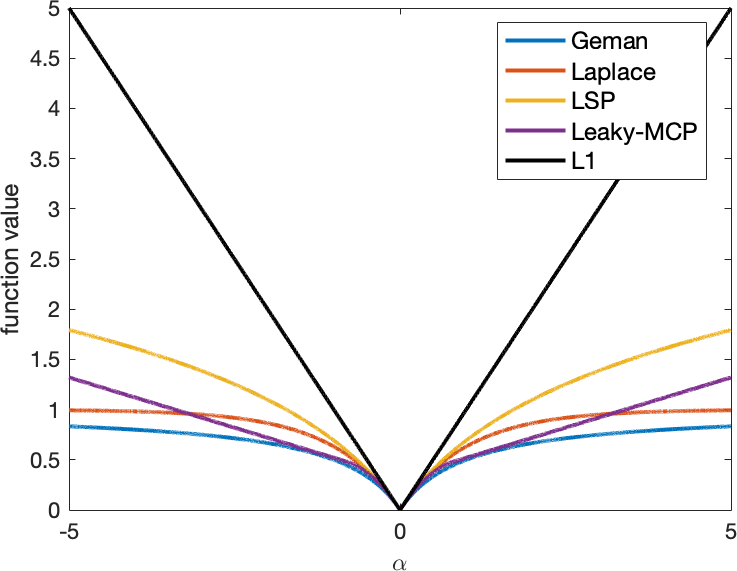
In this section, we make the following Assumption on $\phi$.

Assumption 3.

$\phi(\alpha)$ is a concave and increasing function on $\alpha\geq 0$ with $\phi(0)=0$.

TABLE II: Example nonconvex $\phi$ functions.

	$\phi(\alpha)$
Geman penalty [62]	$\frac{\lvert\alpha\rvert}{\theta+\lvert\alpha\rvert}$
Laplace penalty [63]	$1-\exp(-\frac{\lvert\alpha\rvert}{\theta})$
log-sum penalty (LSP) [44]	$\log(1+\lvert x\rvert)$
leaky-minimax concave penalty (MCP) [43]	$\begin{aligned} \begin{cases}-\frac{1}{2}\alpha^{2}+\theta\lvert\alpha\rvert,&0\leq\alpha\leq\theta-\eta\\ \eta\lvert\alpha\rvert+\frac{1}{2}(\theta-\eta)^{2},&\alpha>\theta-\eta\end{cases}\end{aligned}$

Table II shows the corresponding $\phi$ functions for some popular nonconvex penalties. With a nonconvex loss $\phi$, problem (13) becomes

$$\min_{X}\dot{R}(X)\equiv \sum\nolimits_{\tau=1}^{m}\phi\big{(}\lvert\text{tr}(X{{}^{\top}}Q_{\tau}X)-t_{\tau}\rvert\big{)}$$ (23)

$$+\frac{\gamma}{2}\text{tr}(X^{\top}\!AX)+\frac{\lambda}{2}\|X\|_{F}^{2}.$$

Because of the nonconvexity of $\phi$, optimization of (23) is even more difficult. Again, we will alleviate this problem with the use of MM.

4.1 Convex Surrogate and Its Optimization

For any $\tilde{X}\in{\mathbb{R}}^{n\times r}$, the following Lemma bounds $\dot{R}(X_{k}+\tilde{X})$, where $\dot{R}$ is the objective in (23).

Lemma 4.

For any $\tilde{X}\in{\mathbb{R}}^{n\times r}$,

$$\dot{R}(X_{k}+\tilde{X})\leq \frac{\gamma}{2}\text{tr}((2X_{k}+\tilde{X})^{\top}C\tilde{X})+\dot{c}_{k}$$ (24)

$$+\sum\nolimits_{\tau=1}^{m}(q_{k})_{\tau}|\text{tr}(\tilde{X}^{\top}Q_{\tau}\tilde{X})|$$

$$+\sum\nolimits_{\tau=1}^{m}(q_{k})_{\tau}|\text{tr}((2\tilde{X}\!+\!X_{k})^{\top}\!Q_{\tau}\!X_{k})\!-\!t_{\tau}|,$$

where $(q_{k})_{\tau}=\phi^{\prime}\big{(}|\text{tr}(X_{k}^{\top}Q_{\tau}X_{k})-t_{\tau}|\big{)}$, and $\dot{c}_{k}=\sum\nolimits_{\tau=1}^{m}(\phi(|\text{tr}(X_{k}^{\top}Q_{\tau}X_{k})-t_{\tau}|)-(q_{k})_{\tau}\text{tr}(X_{k}^{\top}Q_{\tau}X_{k})-t_{\tau}|)+\frac{\gamma}{2}\text{tr}(X_{k}^{\top}CX_{k})$.

Combining with Lemma 2, we construct a new surrogate as follows:

Proposition 4.

$\dot{R}({\tilde{X}}+X_{k})\leq\dot{H}_{k}({\tilde{X}};X_{k})$, where

$$\dot{H}_{k}({\tilde{X}};X_{k}) =\text{tr}(\tilde{X}^{\top}(B\tilde{X}+\gamma CX_{k}))$$

$$+2\sum\nolimits_{\tau=1}^{m}|\text{tr}(\tilde{X}^{\top}\dot{Q}_{\tau}X_{k})+(\dot{b}_{k})_{\tau}|+\dot{c}_{k},$$

$\dot{Q}_{\tau}=(q_{k})_{\tau}Q_{\tau}$, $B$ and $C$ as defined in Proposition 2, and $(\dot{b}_{k})_{\tau}\!=\!\frac{1}{2}(q_{k})_{\tau}\big{(}\text{tr}(X_{k}^{\top}Q_{\tau}X_{k})\!-\!t_{\tau}\big{)}$. Equality holds iff $\tilde{X}=\mathbf{0}$.

Obviously, $\dot{H}_{k}({\tilde{X}};X)$ is convex w.r.t. ${\tilde{X}}$. Moreover, it can be easily seen that the three desirable properties for MM surrogates (Section 2.1) are also satisfied by $\dot{H}_{k}({\tilde{X}};X)$. As in Section 3.1.2, the optimization subproblem for $\dot{H}_{k}$ can be reformulated as:

$$\min\nolimits_{\tilde{X}}\; \;\text{tr}(\tilde{X}^{\top}(Q\tilde{X}+\gamma CX_{k}))+2\sum\nolimits_{\tau=1}^{m}|e_{\tau}|+\dot{c}_{k},$$

s.t. $$\;e_{\tau}=\text{tr}(\tilde{X}^{\top}\dot{Q}_{\tau}X_{k})+(\dot{b}_{k})_{\tau}\quad\tau=1,\dots,m.$$

This is of the same form as (3.1.2), and so can be solved analogously with ADMM. Let

$$\dot{B}_{k}\! =\!2Q+\rho\sum\nolimits_{\tau=1}^{m}\dot{Q}_{\tau}X_{k}X_{k}^{\top}\dot{Q}_{\tau}^{\top},$$

$$\dot{C}_{k}\! =\!\gamma C\!+\!\sum\nolimits_{\tau=1}^{m}(\rho(\text{tr}({\tilde{X}}_{t}^{\top}\dot{Q}_{\tau}X_{k})\!-\!e_{\tau}\!+\!(\dot{b}_{k})_{\tau}){-}\nu_{\tau})\dot{Q}_{\tau},$$

$$\dot{e}^{\pm}_{\tau}\! =\!\text{tr}({\tilde{X}}_{t+1}^{{{}^{\top}}}\dot{Q}_{\tau}X_{k})+(\dot{b}_{k})_{\tau}+\nicefrac{{\nu_{\tau}\pm 2}}{{2\rho}},$$

$$\!\!\!\!\dot{\mathcal{D}}_{k}(\{\nu_{\tau}\})\! =\!\frac{\gamma}{2}\sum\nolimits_{\tau=1}^{m}\nu_{\tau}(\text{tr}((CX_{k})^{\top}Q^{-1}\dot{Q}_{\tau}X_{k})-\frac{2}{\gamma}(\dot{b}_{k})_{\tau})$$

$$- \frac{1}{4}\sum\nolimits_{\tau_{1}=1}^{m}\!\sum\nolimits_{\tau_{2}=1}^{m}\!\nu_{\tau_{1}}\nu_{\tau_{2}}(\text{tr}((\dot{Q}_{\tau_{1}}X_{k})^{\top}Q^{-1}(\dot{Q}_{\tau_{2}}X_{k}))$$

$$- \frac{\gamma^{2}}{4}\text{tr}((CX_{k})^{\top}Q^{-1}(CX_{k}))+\dot{c}_{k}.$$

The resultant procedure, which consists of Algorithms 3 and 4, are slight modifications of Algorithms 1 and 2, respectively. The main difference is on how $\dot{Q}_{\tau}$ (resp. $Q_{\tau}$) and $(\dot{b}_{k})_{\tau}$ (resp. $(b_{k})_{\tau}$) are computed. Thus, the complexity results in Table I still apply.

Algorithm 3 Variant of Algorithm 1 for nonconvex loss.

0:  pre-defined tolerance $\epsilon_{k}$.

1:  Initialization: $t=1,\tilde{X}_{1}=0$;

2:  while $\delta_{k}({\tilde{X}}_{t},\{(\tilde{\nu}_{\tau})_{t}\})\geq\epsilon_{k}$ do

3:     update ${\tilde{X}}_{t+1}={\tilde{X}}_{t}-\dot{B}_{k}^{-1}(2Q{\tilde{X}}_{t}+\dot{C}_{k}X_{k})$;

4:     for $\tau=1,\dots,m$ do

5:        update $(\dot{e}_{\tau})_{t+1}=\max(0,\dot{e}^{-}_{\tau})+\min(0,\dot{e}^{+}_{\tau})$;

6:        $(\nu_{\tau})_{t+1}\!=\!(\nu_{\tau})_{t}\!+\!\frac{1}{\rho}(\dot{e}_{\tau}\!-\!\text{tr}(X_{k}^{{{}^{\top}}}\dot{Q}_{\tau}{\tilde{X}}_{t\!+\!1})\!-\!(\dot{b}_{k})_{\tau})$;

7:     end for

8:     compute $\delta_{k}({\tilde{X}}_{t},\{(\tilde{\nu}_{\tau})_{t}\})$, the upper-bound on inexactness;

9:     $t=t+1$;

10:  end while

11:  return  ${\tilde{X}}_{t}$.

Algorithm 4 SDP-RL for nonconvex loss.

1:  Initialization: $X_{1}=0$.

2:  for $k=1,\ldots,K$ do

3:     obtain ${\tilde{X}}_{t}$ via Algorithm 3 with tolerance $\epsilon_{k}$;

4:     update $X_{k+1}={\tilde{X}}_{t}+X_{k}$;

5:  end for

6:  return  $X_{K+1}$.

4.2 Convergence Analysis

In Section 3.2, the convex $\ell_{1}$-loss is considered, and the critical points can be characterized by the subgradient of $\ell_{1}$. However, the subgradient cannot be used on a nonconvex loss $\phi$. The following first introduces generalizations of the subgradient and critical point.

Definition 4.1 ([64]).

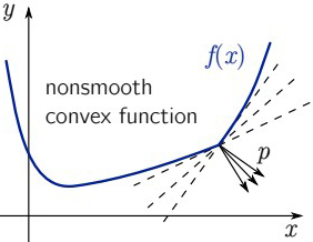
The Frechet subdifferential of $f$ at $x$ is $\hat{\partial}f(x)=\{u:\lim\nolimits_{y\neq x}\inf_{y\rightarrow x}\frac{f(y)-f(x)-u^{\top}(y-x)}{\|y-x\|_{2}}\geq 0\}$. The limiting subdifferential (or simply subdifferential) of $f$ at $x$ is $\partial f(x)=\{u:\exists x_{k}\rightarrow x,f(x_{k})\rightarrow f(x),u_{k}\in\hat{\partial}f(x_{k})\!\rightarrow\!u,\text{ as }k\rightarrow\infty\}$.

When $f$ is smooth, $\partial f(x)$ reduces to the gradient. When $f$ is nonsmooth but convex, $\partial f(x)$ is the set of all subgradients of $f$ at $x$. An example is shown in Figure 2.

(a) subgradient.

(b) subdifferential.

Figure 2: Plots of subgradient and Frechet subdifferential, where $p$ denotes the normal direction.

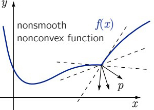
Definition 4.2 ([64]).

$x$ is a critical point of $f$ if $0\in\partial f(x)$.

We make the following Assumption on $\dot{R}$, which is analogous to Assumption 1 on $R$.

Assumption 4.

$\underset{\|X\|_{F}\rightarrow\infty}{\lim}\!\!\!\!\dot{R}(X)=\infty$ and $\underset{X}{\inf}\;\dot{R}(X)>-\infty$.

Convergence to critical points is then ensured by the following Theorem. Its proof can be easily adapted from that of Theorem 1.

Theorem 2.

With Assumptions 2, 3 and 4, for the sequence $\{X_{k}\}$ generated from Algorithm 4, we have (i) $\{X_{k}\}$ is bounded; (ii) any limit point of $\{X_{k}\}$ is a critical point of $\dot{R}$.

5 Example Robust SDP Applications

In this section, we illustrate a number of applications that can be robustified with the proposed formulations. For simplicity, we focus on the $\ell_{1}$ loss. These can be easily extended to the nonconvex loss in Section 4.

5.1 Positive Semi-Definite Matrix Completion

The first example is on completing a partially observed PSD matrix [7, 8]. This has applications in, e.g., learning of the user-item matrix recommender systems [5] and multi-armed bandit problems [9]. Let the data matrix be $O$, and $\Omega\equiv\{(i,j)\}$ be the set of indices for the observed $O_{ij}$’s. PSD matrix completion can be formulated as finding a $Z\in{\mathbb{S}}_{+}$ via the following optimization problem:

$$\min\limits_{Z\in{\mathbb{S}}_{+}}\sum\nolimits_{(i,j)\in\Omega}\frac{1}{2}(Z_{ij}-O_{ij})^{2}+\frac{\gamma}{2}\text{tr}(Z),$$ (25)

where the first term measures the loss, and the second term encourages the matrix $Z$ to be low-rank (note that $\|Z\|_{*}=\text{tr}(Z)$ for $Z\in{\mathbb{S}}_{+}$). Let $Q^{(i,j)}$ be a matrix of zeros except that $Q^{(i,j)}_{ij}=1$. Problem (25) is then of the form in (3), with $Q_{\tau}=Q^{(i,j)}$, $t_{\tau}=O_{ij}$, and $A=\mathbf{0}$.

The square loss in (25) may not be appropriate in some applications. For example, the love-and-hate attack [40] in recommender systems flips high ratings to low values, and vice versa [41]. The corrupted ratings then become large outliers, and using the square loss can lead to significant performance degradation [32, 41]. To improve robustness, we replace the square loss by the $\ell_{1}$-loss, leading to

$$\min\limits_{Z\in{\mathbb{S}}_{+}}\sum\nolimits_{(i,j)\in\Omega}|Z_{ij}-O_{ij}|+\frac{\gamma}{2}\text{tr}(Z).$$ (26)

Let $Z=XX^{\top}$. It is easy to see that $Z_{ij}=x_{i}^{\top}x_{j}$, where $x_{i}^{\top}$ is the $i$th row of $X$, and $\text{tr}(Z)=\|X\|^{2}_{F}$. Problem (26) can then be rewritten as:

$$\min_{X}\sum\nolimits_{(i,j)\in\Omega}|\text{tr}(X^{\top}Q^{(i,j)}X)-O_{ij}|+\frac{\gamma}{2}\|X\|^{2}_{F}.$$ (27)

5.1.1 Utilizing Data Sparsity

Algorithms 1 and 2 can be directly used to solve (27). However, each iteration of Algorithm 1 has to construct $Q_{\tau}$ (defined in Lemma 2) and invert $\tilde{B}_{k}$ (in (18)). A straightforward implementation leads to $O(n^{2}r)$ time and $O(n^{2})$ space. Recall that the partially observed matrix $O$ is sparse. In the following, we show how data sparsity can be used to speed up optimization of (27), as has been demonstrated in other matrix learning problems [41, 31].

Proposition 5.

Let $\tilde{x}^{\top}_{i}$ (resp., $(x_{k})^{\top}_{i}$) be the $i$th row of $\tilde{X}$ (resp., $X_{k}$). The objective in (3.1.2) can be rewritten as

$$\min\nolimits_{{\tilde{X}}}\; \;\frac{\gamma}{2}\|{\tilde{X}}\|_{F}^{2}+\frac{1}{2}\|\Lambda^{r}{\tilde{X}}\|_{F}^{2}+\frac{1}{2}\|\Lambda^{c}{\tilde{X}}\|_{F}^{2}$$

$$+\lambda\text{tr}({\tilde{X}}^{\top}X_{k})+2\sum\nolimits_{\tau=1}^{m}\lvert e_{\tau}\rvert$$

s.t. $$\;e_{ij}=\tilde{x}_{i}^{\top}(x_{k})_{j}+(b_{k})_{ij},\;\forall(i,j)\in\Omega,$$

where $\Lambda^{r}$ and $\Lambda^{c}$ are as defined in Proposition 1, and $(b_{k})_{ij}=\frac{1}{2}((x_{k})_{i}^{\top}(x_{k})_{j}-O_{ij})$.

Using Proposition 5, the ADMM updates for $\tilde{X}$ and $e_{\tau}$ (in (18) and (19), respectively) become

$${\tilde{X}}_{t+1} ={\tilde{X}}_{t}-\hat{B}_{k}^{-1}((\Lambda^{r}+\Lambda^{c}+\gamma I){\tilde{X}}+\hat{C}_{k}X_{k}),$$ (28)

$$(e_{ij})_{t+1} =\max\left(0,\hat{e}^{-}_{\tau}\right)+\min\left(0,\hat{e}^{+}_{\tau}\right),$$

where $\hat{B}_{k}=\Lambda^{r}+\Lambda^{c}+\gamma I+{\Omega\odot(\rho X_{k}X_{k}^{\top})}$, $\hat{C}_{k}=\gamma I\!+\!\sum\nolimits_{(i,j)\in\Omega}(\rho(\tilde{x}_{i}^{\top}(x_{k})_{j}\!-\!e_{ij}\!+\!(b_{k})_{ij})\!-\!\nu_{ij})Q^{(i,j)}$, $\hat{e}^{\pm}_{ij}=(\tilde{x}_{t+1})_{i}^{\top}(x_{k})_{j}+(b_{k})_{ij}+(\nu_{ij}\pm 2)/\rho$. To update ${\tilde{X}}_{t}$ in (28) (and also $X_{k}$ in Algorithm 2), we only need to store sparse matrices ($\hat{B}_{k}$ and $\hat{C}_{k}$) and diagonal matrices ($\Lambda^{r}$ and $\Lambda^{c}$). Moreover, the second term on the R.H.S. of (28), which involves inversion of $\hat{B}_{k}$, can be computed in $O(nr^{2}+\text{nnz}(\Omega))$ time using conjugate gradient descent [28]. Finally, each $(\nu_{\tau})_{t+1}$ is updated as $(\nu_{ij})_{t+1}\!=\!(\nu_{ij})_{t}+(e_{ij}\!-\tilde{x}_{i}^{\top}(x_{k})_{j}+(b_{k})_{ij})/\rho$ in $O(r)$ time. Thus, each ADMM iteration in Algorithm 1 only takes $O(nr^{2}+\text{nnz}(\Omega)r)$ time and $O(nr+\text{nnz}(\Omega))$ space, which is much faster than the other SDP methods for the $\ell_{1}$ loss (see Table I).

5.2 Robust NPKL

In nonparametric kernel learning (NPKL) [65], one tries to learn a kernel matrix from data. In this section, we adopt the formulation in [18, 19]. Let ${\mathcal{T}}={\mathcal{M}}\cup{\mathcal{C}}$, where ${\mathcal{M}}$ is the set containing sample pairs that should belong to the same class (must-link set), and ${\mathcal{C}}$ is the set containing sample pairs that should not belong to the same class (cannot-link set). This can be encoded by the matrix $O$, such that $O_{ij}=1$ for a must-link $(i,j)$ pair, and $O_{ij}=0$ for a cannot-link pair. The NPKL problem is formulated as the following SDP:

$$\min\nolimits_{Z\in{\mathbb{S}}^{+}}\sum\nolimits_{(i,j)\in{\mathcal{T}}}\big{(}Z_{ij}-O_{ij}\big{)}^{2}+\frac{\gamma}{2}\text{tr}(ZL),$$ (29)

where $Z$ is the target kernel matrix and $L$ is the Laplacian of the $k$-nearest neighbor graph of data. The first term in (29) measures the difference between $Z_{ij}$ and $O_{ij}$, while the second term encourages smoothness on the data manifold by aligning $Z$ with $L$.

The must-links and cannot-links are usually provided by users or crowdsourcing. These can be noisy as there may be human errors and spammers/attackers on crowdsourcing platforms [39]. As in Section 5.1, we let $Z=XX^{\top}$ and obtain the following robust NPKL formulation:

$$\min_{X}\!\!\!\sum_{(i,j)\in{\mathcal{T}}}\!\!\!|\text{tr}(X{{}^{\top}}Q^{(i,j)}X)-O_{ij}|+\frac{\gamma}{2}\text{tr}(X{{}^{\top}}LX)+\frac{\lambda}{2}\|X\|_{F}^{2},$$

where $Q^{(i,j)}$ is the same as in Section 5.1. Obviously, this is again of the same form as (3.1.2), with $Q_{\tau}=Q^{(i,j)}$, $t_{\tau}=O_{ij}$ and $A=L$. When $|{\mathcal{T}}|$ is small, data sparsity can also be utilized as in Section 5.1.1.

5.3 Robust CMVU

Maximum variance unfolding (MVU) [16] is an effective dimensionality reduction method. It produces a low-dimensional data representation by simultaneously maximizing the variance of the embedding and preserving the local distances of the original data. Colored maximum variance unfolding (CMVU) is a “colored” variant of MVU [17], with class label information. Let

$$\bar{K}=HTH,$$ (30)

where $T$ is a kernel matrix on labels, and $H$ (with $H_{ij}=\mathbbm{1}(i=j)-{\frac{1}{n}}$) is a matrix that centers the data and labels in the feature space. CMVU is formulated as the following optimization problem:

$$\min\limits_{Z\in{\mathbb{S}}^{+}}\sum\nolimits_{(i,j)\in\Omega}\big{(}Z_{ii}\!+\!Z_{jj}\!-\!2Z_{ij}\!-\!d_{ij}\big{)}^{2}\!\!-\frac{\gamma}{2}\text{tr}(Z\bar{K}),$$ (31)

where $d_{ij}$ is the squared Euclidean distance between the $i$th and $j$th samples in the original space, $\Omega$ is a set of neighbor pairs whose distances are to be preserved in the embedding, and $\gamma$ controls the tradeoff between distance preservation (the first term) and dependence maximization (second term).

Often, outliers and corrupted samples are introduced during data collection. Again, by letting $Z=XX^{\top}$, we have the following robust CMVU formulation which is of the same form as (3.1.2):

$$\min_{X}\!\!\sum\nolimits_{(i,j)\in\Omega}\lvert\text{tr}(X^{\top}\!\hat{Q}^{(i,j)}X)\!-\!d_{ij}\rvert\!-\!\frac{\gamma}{2}\text{tr}(X^{\top}\!\bar{K}X)\!+\!\frac{\lambda}{2}\|X\|_{F}^{2},$$

where $\hat{Q}^{(i,j)}=Q^{(i,i)}+Q^{(j,j)}-Q^{(i,j)}-Q^{(i,j)}$ and $Q^{(i,j)}$ is the same as that in Section 5.1. This again is the same form as (13), with $Q_{\tau}=\hat{Q}^{(i,j)}$, $t_{\tau}=d_{ij}$ and $A=-\bar{K}$. When $|\Omega|$ is small, data sparsity can also be utilized as in Section 5.1.1.

5.4 Sparse PCA

Sparse PCA [13, 15] is a popular method to extract sparse principal components from the data, i.e., sparse vectors $x$ that maximizes $x{{}^{\top}}\Sigma x$ for a given covariance matrix $\Sigma\in{\mathbb{R}}^{n\times n}$. It can be relaxed to the following SDP [13]:

$$\min\nolimits_{Z\in{\mathbb{S}}_{+}}-\text{tr}(Z\Sigma)\quad\text{s.t.}\quad\text{tr}(Z)=1,\;\|Z\|_{1}\leq k,$$ (32)

where $k$ is a hyper-parameter controlling the sparsity.

As in previous sections, we let $Z=XX^{\top}$. Note that $\text{tr}(Z)=\|X\|_{F}^{2}$ and $|Z_{ij}|=|\text{tr}(X^{{}^{\top}}Q^{(i,j)}X)|$, where $Q^{(i,j)}$ is in (27). By moving the constraints in (32) to the objective, it can be reformulated as

$$\min_{X}\sum\nolimits_{i,j}\lvert\text{tr}(X^{{}^{\top}}Q^{(i,j)}X)\rvert+\frac{\lambda}{2}\|X\|_{F}^{2}-\frac{\gamma}{2}\text{tr}(X{{}^{\top}}\Sigma X),$$ (33)

which is the same as (13), with $Q_{\tau}\!=\!Q^{(i,j)}$, $t_{\tau}\!=\!0$ and $A\!=\!-\!\Sigma$.

5.5 Symmetric NMF

Symmetric nonnegative matrix factorization (NMF) [66, 67] aims to factorize a non-negative and symmetric matrix $O$ by solving

$$\min\nolimits_{X}\frac{1}{2}\|O-XX^{\top}\|_{F}^{2}\quad\text{s.t.}\quad X_{ij}\geq 0.$$ (34)

SNMF is popular in clustering analysis [68] as it can effectively identify low-dimensional data representations.

Again, the square loss in (34) may not be appropriate in some scenarios (for example, noisy observed data in clustering, which affect the observed $O_{ij}$’s), leading to degraded performance. Similar to Section 5.1, we have the following robust SNMF formulation:

$$\min_{X}\sum\nolimits_{i,j}|\text{tr}(X^{\top}Q^{(i,j)}X)-O_{ij}|+\frac{\lambda}{2}\|X\|^{2}_{F},$$ (35)

which is of the form in (13) with $Q_{\tau}=Q^{(i,j)}$, $t_{\tau}=O_{ij}$ and $A=\mathbf{0}$.

TABLE III: Testing RMSEs and CPU time (sec) on synthetic data with different matrix sizes ($m$). The number in brackets is the percentage of observed elements. ‘-’ indicates the algorithm fails to converge in $10^{4}$ seconds.

loss	algorithm	$m=500$ ($12.43\%$)		$m=1000$ ($6.91\%$)		$m=1500$ ($4.88\%$)		$m=2000$ ($3.80\%$)
		testing	CPU	testing	CPU	testing	CPU	testing	CPU
		RMSE	time	RMSE	time	RMSE	time	RMSE	time
square	FW	3.2$\pm$0.1	2$\pm$1	3.8$\pm$0.1	5$\pm$1	4.2$\pm$0.1	8$\pm$1	4.4$\pm$0.1	12$\pm$1
	nmAPG	0.964$\pm$0.006	2$\pm$1	0.785$\pm$0.004	5$\pm$1	0.637$\pm$0.008	6$\pm$1	0.615$\pm$0.008	19$\pm$2
	L-BFGS	0.964$\pm$0.006	2$\pm$1	0.794$\pm$0.006	4$\pm$1	0.638$\pm$0.006	6$\pm$1	0.615$\pm$0.007	17$\pm$2
	ADMM($\ell_{1}$)	0.494$\pm$0.008	54$\pm$9	0.394$\pm$0.008	564$\pm$48	0.356$\pm$0.006	1546$\pm$38	0.332$\pm$0.006	2387$\pm$44
	SDPLR	0.497$\pm$0.008	5064$\pm$135	0.396$\pm$0.004	6784$\pm$246	-	-	-	-
$\ell_{1}$	SDPNAL+	0.488$\pm$0.006	397$\pm$45	0.388$\pm$0.006	1562$\pm$189	-	-	-	-
	SDP-RL-dense	0.246$\pm$0.004	46$\pm$6	0.216$\pm$0.003	436$\pm$24	0.172$\pm$0.002	1588$\pm$46	0.164$\pm$0.002	2658$\pm$63
	SDP-RL($\ell_{1}$)	0.246$\pm$0.004	3$\pm$1	0.216$\pm$0.003	11$\pm$1	0.172$\pm$0.002	23$\pm$2	0.164$\pm$0.002	37$\pm$2
leaky-MCP	SDP-RL(MCP)	0.126$\pm$0.002	6$\pm$1	0.121$\pm$0.002	16$\pm$2	0.117$\pm$0.002	27$\pm$3	0.113$\pm$0.001	46$\pm$2

(a) $m=500$.

(b) $m=1000$.

(c) $m=1500$.

(d) $m=2000$.

Figure 3: Convergence of the testing RMSE vs CPU time (sec) of various algorithms on synthetic data. SDPLR and SDPNAL+ are too slow on $m=1500$ and $2000$, thus are not shown.

6 Experiments

In this section, experiments are performed on five machine learning applications, namely, PSD matrix completion (Section 6.1), non-parametric kernel learning (Section 6.2), maximum variance unfolding (Section 6.3), sparse PCA (Section 6.4), and symmetric NMF (Section 6.5). Depending on the loss function and whether the matrix variate is factored, the following SDP solvers will be compared:

1. Solver for SDP problem (3) (i.e., square loss and matrix variate is not factored):

   1. FW [5], which uses the Frank-Wolfe algorithm [6];

2. Solvers for problem (4) (i.e., square loss and factored matrix variate):

   1. nmAPG [57], which uses the state-of-the-art accelerated gradient descent algorithm; and

   2. L-BFGS [28], which uses the popular quasi-Newton solver for smooth minimization problem.

3. Solvers for SDP problem with $\ell_{1}$-loss, i.e., (22):

   1. ADMM($\ell_{1}$), which solves the nonsmooth but convex problem with ADMM [50];

   2. SDPLR [21], which considers (22) and solves with the augmented Lagrangian method;

   3. SDPNAL+ [20], which also solves (22) but with the Newton-CG augmented Lagrangian method.

4. Solvers for problem (13) (i.e., $\ell_{1}$-loss and factored matrix variate):

   1. SDP-RL($\ell_{1}$): the proposed Algorithm 2, and data sparsity is utilized as discussed in Section 5.1.1;

   2. SDP-RL-dense, which is the same as SDP-RL($\ell_{1}$) except that data sparsity is not utilized;

5. Solver for problem (23) (i.e., nonconvex loss and factored matrix variate):

   1. SDP-RL(MCP), the proposed Algorithm 4 which uses the leaky-MCP loss in Table II, with $\theta=5$ and $\eta=0.05$. As reported in [59, 69, 41], the nonconvex losses in Table II usually have similar performance.

For all the SDP-RL variants above, ADMM is used as the solver for the convex surrogate. We set the maximum number of ADMM iterations to $1000$, and a tolerance $\epsilon_{k}$ of $\max(10^{-8},c_{0}/k^{b_{0}})$ as in Remark 1, where $b_{0}=1.5$.

All these algorithms are implemented in Matlab. Each of these is stopped when the relative change of objective values in successive iterations is smaller than $10^{-5}$ or when the number of iterations reaches $2000$. To reduce statistical variability, results are averaged over five repetitions. Results for the best-performing method and those that are not significantly worse (according to the pairwise t-test with 95% significance level) are highlighted. Experiments are run on a PC with a 3.07GHz CPU and 32GB RAM.

6.1 PSD Matrix Completion

TABLE IV: Testing RMSEs and CPU time (sec) on synthetic data with different observation sampling ratios ($s$). The number in brackets is the percentage of observed elements.

loss	algorithm	$s=1$ ($1.90\%$)		$s=2$ ($3.80\%$)		$s=4$ ($7.60\%$)		$s=8$ ($15.20\%$)
		testing	CPU	testing	CPU	testing	CPU	testing	CPU
		RMSE	time	RMSE	time	RMSE	time	RMSE	time
square	nmAPG	0.896$\pm$0.008	17$\pm$3	0.615$\pm$0.008	19$\pm$2	0.442$\pm$0.003	21$\pm$2	0.258$\pm$0.006	25$\pm$3
	L-BFGS	0.896$\pm$0.007	16$\pm$1	0.615$\pm$0.007	17$\pm$2	0.443$\pm$0.003	21$\pm$3	0.256$\pm$0.007	27$\pm$4
$\ell_{1}$	ADMM($\ell_{1}$)	0.436$\pm$0.008	1638$\pm$56	0.332$\pm$0.006	2387$\pm$44	0.264$\pm$0.005	3765$\pm$38	0.189$\pm$0.003	5582$\pm$87
	SDP-RL($\ell_{1}$)	0.256$\pm$0.004	36$\pm$3	0.164$\pm$0.002	37$\pm$2	0.109$\pm$0.001	55$\pm$5	0.084$\pm$0.003	78$\pm$6
leaky-MCP	SDP-RL(MCP)	0.168$\pm$0.001	50$\pm$3	0.113$\pm$0.001	46$\pm$2	0.077$\pm$0.002	67$\pm$6	0.053$\pm$0.002	121$\pm$8

TABLE V: Testing RMSEs and CPU time (sec) on synthetic data with different fractions of outlying entries ($o$).

loss	algorithm	$o=0$		$o=0.025$		$o=0.05$		$o=0.10$		$o=0.20$
		testing	CPU	testing	CPU	testing	CPU	testing	CPU	testing	CPU
		RMSE	time	RMSE	time	RMSE	time	RMSE	time	RMSE	time
square	nmAPG	0.005$\pm$0.001	10$\pm$2	0.228$\pm$0.003	17$\pm$2	0.309$\pm$0.002	16$\pm$1	0.422$\pm$0.003	16$\pm$3	0.590$\pm$0.002	17$\pm$3
	L-BFGS	0.005$\pm$0.001	11$\pm$1	0.228$\pm$0.003	14$\pm$2	0.309$\pm$0.002	15$\pm$1	0.422$\pm$0.003	14$\pm$1	0.590$\pm$0.002	15$\pm$3
$\ell_{1}$	ADMM($\ell_{1}$)	0.009$\pm$0.002	2846$\pm$123	0.192$\pm$0.003	2873$\pm$83	0.199$\pm$0.003	2870$\pm$62	0.222$\pm$0.002	2893$\pm$146	0.269$\pm$0.002	2869$\pm$41
	SDP-RL($\ell 1_{1}$)	0.007$\pm$0.001	39$\pm$3	0.110$\pm$0.002	44$\pm$3	0.113$\pm$0.001	40$\pm$4	0.142$\pm$0.002	37$\pm$3	0.161$\pm$0.002	34$\pm$2
leaky-MCP	SDP-RL(MCP)	0.007$\pm$0.001	47$\pm$4	0.109$\pm$0.001	51$\pm$3	0.111$\pm$0.001	47$\pm$3	0.119$\pm$0.001	44$\pm$7	0.134$\pm$0.001	41$\pm$3

TABLE VI: Testing RMSEs and CPU time (sec) on synthetic data with different maximum outlier amplitudes ($\sigma$).

loss	algorithm	$\sigma=2.5$		$\sigma=5.0$		$\sigma=10.0$		$\sigma=20.0$
		testing	CPU	testing	CPU	testing	CPU	testing	CPU
		RMSE	time	RMSE	time	RMSE	time	RMSE	time
square	nmAPG	0.170$\pm$0.001	16$\pm$1	0.309$\pm$0.002	16$\pm$1	0.615$\pm$0.008	19$\pm$2	1.36$\pm$0.01	22$\pm$1
	L-BFGS	0.170$\pm$0.001	15$\pm$3	0.309$\pm$0.002	15$\pm$1	0.615$\pm$0.007	17$\pm$2	1.36$\pm$0.02	17$\pm$3
$\ell_{1}$	ADMM($\ell_{1}$)	0.191$\pm$0.002	2868$\pm$141	0.199$\pm$0.003	2870$\pm$62	0.332$\pm$0.006	2837$\pm$84	0.418$\pm$0.008	2906$\pm$45
	SDP-RL($\ell_{1}$)	0.114$\pm$0.001	49$\pm$7	0.113$\pm$0.001	40$\pm$4	0.164$\pm$0.002	37$\pm$2	0.183$\pm$0.002	35$\pm$3
leaky-MCP	SDP-RL(MCP)	0.113$\pm$0.001	60$\pm$6	0.111$\pm$0.001	47$\pm$3	0.113$\pm$0.001	46$\pm$2	0.112$\pm$0.001	43$\pm$2

In this section, experiments are performed on PSD matrix completion (Section 5.1) in the context of recommender systems. Following [32], we mimic the love/hate attacks, and some ratings in the synthetic data are randomly set to the highest/lowest values.

The ground-truth matrix $M$ is generated as a low-rank matrix $VV^{\top}$, where $V\in\mathbb{R}^{m\times r}$ with entries sampled i.i.d. from $\mathcal{N}(0,1)$. This is then corrupted as $M^{\prime}={M}+N+S$, where $N$ is a noise matrix and $S$ is a sparse matrix modeling large outliers (with $o$ being the fraction of nonzero entries). The entries of $N$ are sampled i.i.d. from $\mathcal{N}(0,0.1)$, while the nonzero entries of $S$ are sampled uniformly from $\{-\sigma,\sigma\}$. We randomly draw $\frac{1}{m}sr\log(m)\%$ of the elements from $M^{\prime}$ as (noisy) observations for training, where $s$ controls the sampling ratio. Half of the remaining uncorrupted entries in $M$ are used for validation (hyper-parameter tuning) and the rest for testing. We experiment with matrix size $m\in\{500$, $1000$, $1500$, $2000\}$, and set the ranks for all factorization-based methods to the ground-truth (i.e., 5). The other parameters are set as $o=0.05$, $s=2$ and $\sigma=10$.

Let $XX^{\top}$ be the matrix recovered and $M$ be the clean ground-truth matrix. For performance evaluation, we use (i) the testing root mean squared error (RMSE): $\sqrt{\frac{1}{\|\Omega_{\text{test}}\|_{1}}\sum\nolimits_{(i,j)\in\Omega_{\text{test}}}(M_{ij}-(XX^{\top})_{ij})^{2}}$; and (ii) CPU time.

6.1.1 Results

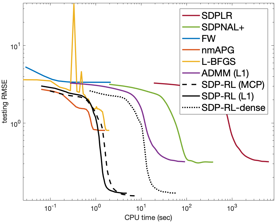
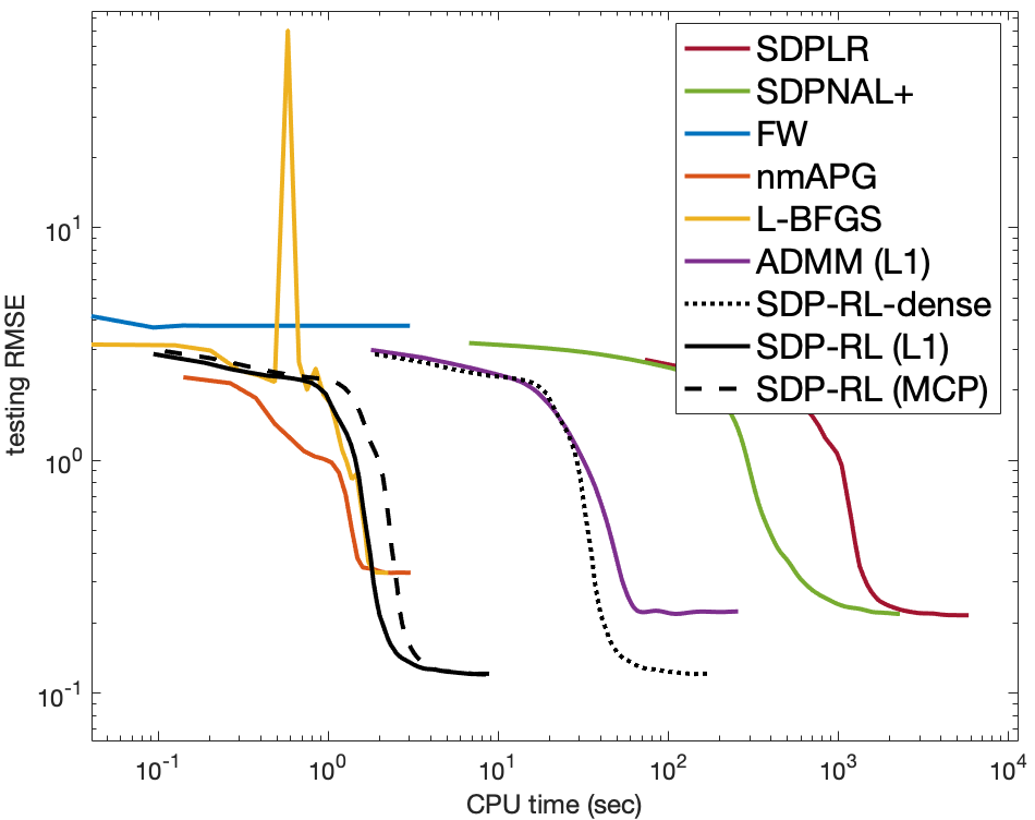
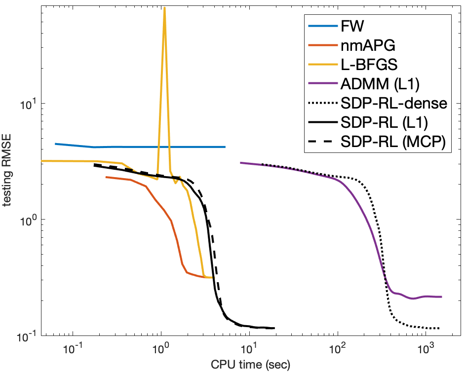
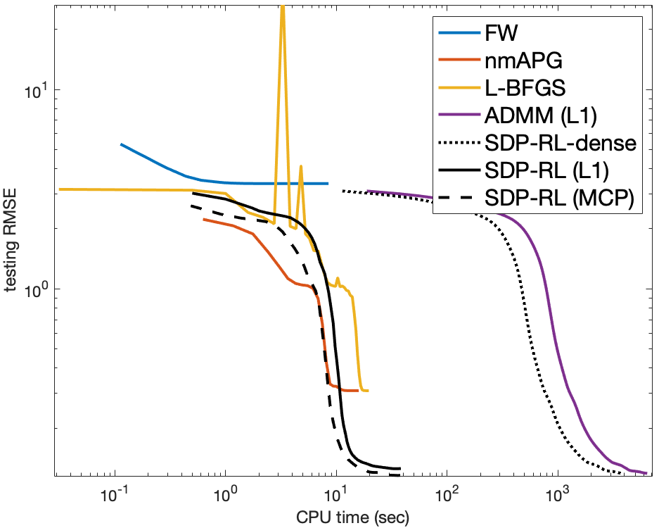
The testing RMSEs and CPU time are in Table III. Convergence of the testing RMSE versus CPU time is in Figure 3. Though methods based on the square loss (FW, nmAPG, and L-BFGS) are very fast, they have much higher testing RMSE’s than methods based on the $\ell_{1}$ and nonconvex losses. In particular, FW yields a much larger testing RMSE than nmAPG and L-BFGS. This is because FW does not explicitly utilize low-rank factorization but relies only on the nuclear-norm regularizer. Moreover, it uses rank-one update in each iteration, and is only as fast as nmAPG and L-BFGS. Thus, FW will not be included in the sequel.

Among algorithms based on the $\ell_{1}$-loss, SDP-RL($\ell_{1}$) is the fastest as it exploits data sparsity. SDP-RL(MCP) yields slightly lower RMSE, but is slightly slower than SDP-RL($\ell_{1}$). As SDPLR and SDPNAL+ have comparable accuracies with ADMM($\ell_{1}$), but are much slower and even fail to converge on large-scale problems. Thus, SDPLR and SDPNAL+ will also be dropped in the subsequent comparisons.

6.1.2 Varying the Number of Observed Entries

We fix the matrix dimension $m=2000$, outlier ratio $o=0.05$, outlier amplitude $\sigma=10$, and vary the sampling ratio $s$ in $\{1$, $2$, $4$, $8\}$. A larger $s$ means that more elements are observed. Table IV shows the testing RMSEs and CPU time. When $s$ increases, the testing RMSE decreases and CPU time increases in general, which agrees with intuition.

6.1.3 Varying the Number of Outlying Entries

We vary the fraction of entries $o$ in the sparse noise matrix $S$ in $\{0,0.025,0.05,0.1,0.2\}$. The other parameters are set as $m=2000$, $r=2$, $s=2$ and $\sigma=5$. Results are shown in Table V. When there is no outlier ($o=0$), nmAPG and L-BFGS perform the best, as they use the square loss which matches with the Gaussian noise generated. As $o$ increases, the testing RMSEs of all algorithms increase as expected. Moreover, using the nonconvex loss leads to more robust results than both the square loss and $\ell_{1}$ loss, particularly when the noise is large.

6.1.4 Varying the Magnitude of Outlying Entries

We vary the magnitude $\sigma$ of outlying entries in $\{2.5,5,10,20\}$. The other parameters are fixed at $m=2000,r=2,s=2$ and $o=0.05$. Results are shown in Table VI. As $\sigma$ increases, the testing RMSEs of most algorithms also increase (as in Section 6.1.3). The only exception is SDP-RL(MCP), whose loss remains almost unchanged. This again shows that SDP-RL(MCP) is more robust.

6.1.5 Varying Tolerance for Subproblem

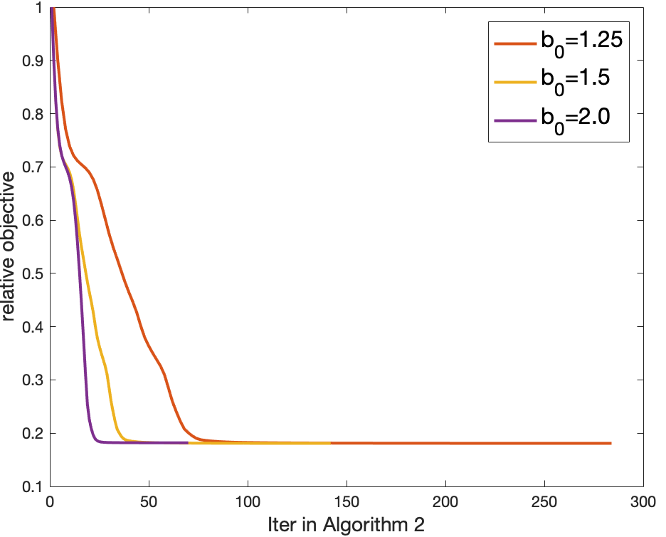
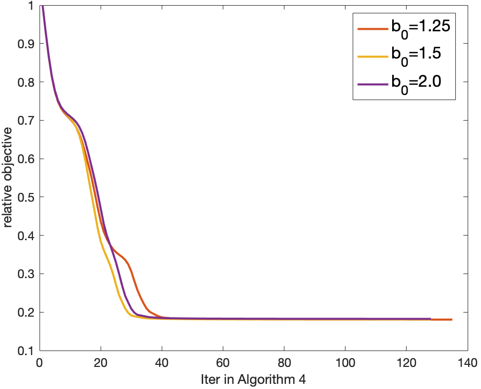
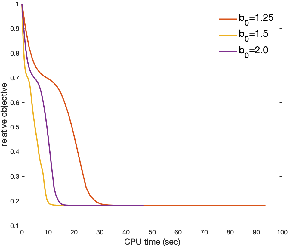
We experiment with the termination criterion of the ADMM solver (in Algorithms 1 and 3). We vary $b_{0}$ in Remark 1 in $\{1.25$, $1.5$, $2.0\}$, and $c_{0}=R(X_{0})$ so that the inexactness scales with the objective value. The other parameters are fixed at $m=2000$, $r=5$, $o=0.25$, $s=2$ and $\sigma=10$.

TABLE VII: Testing RMSEs and CPU time (sec) in the robust NPKL experiment.

loss	algorithm	5% flippd labels		10% flipped labels
		testing RMSE	CPU time	testing RMSE	CPU time
square	SimpleNPKL	0.54$\pm$0.01	407$\pm$24	0.60$\pm$0.01	419$\pm$27
	nmAPG	0.31$\pm$0.01	7$\pm$2	0.35$\pm$0.01	8$\pm$1
	L-BFGS	0.31$\pm$0.01	4$\pm$1	0.35$\pm$0.01	4$\pm$1
$\ell_{1}$	ADMM($\ell_{1}$)	0.23$\pm$0.01	775$\pm$24	0.29$\pm$0.01	784$\pm$19
	SDP-RL($\ell_{1}$)	0.21$\pm$0.01	55$\pm$33	0.28$\pm$0.01	72$\pm$36
leaky-MCP	SDP-RL(MCP)	0.19$\pm$0.02	67$\pm$27	0.26$\pm$0.01	88$\pm$27

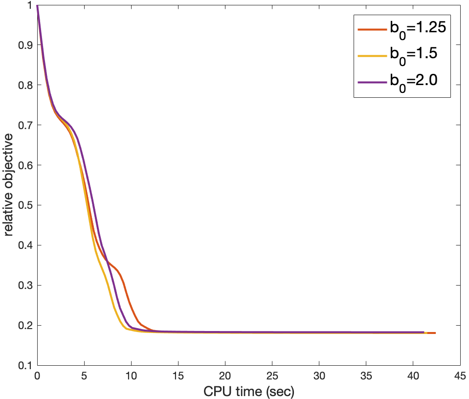
Figure 4 shows convergence of the relative objective $R(X_{k})/R(X_{0})$ vs the number of iterations in Algorithm 2 (resp. Algorithm 4) for SDP-RL($\ell_{1}$) (resp. SDP-RL(MCP)). Recall that each iteration of Algorithm 2 (resp. Algorithm 4) makes one call to Algorithm 1 (resp. Algorithm 3). As can be seen, a larger $b_{0}$ (smaller tolerance) leads to fewer iterations of Algorithm 2 and Algorithm 4. However, solving the ADMM to such a higher precision means more time to solve the surrogate (Table VIII). Figure 5 shows convergence w.r.t. the total CPU time. As can be seen, $b_{0}=1.5$ is a good empirical choice, and we will use this in the sequel.

(a) SDP-RL($\ell_{1}$).

(b) SDP-RL(MCP).

Figure 4: Convergence of relative objective vs number of iterations in Algorithms 2 and 4 at different tolerance on inexactness.

(a) SDP-RL($\ell_{1}$).

(b) SDP-RL(MCP).

Figure 5: Convergence of relative objective vs CPU time (sec) at different tolerance on inexactness.

TABLE VIII: Average per-iteration CPU time (sec) of SDP-RL.

	$b_{0}=1.25$	$b_{0}=1.5$	$b_{0}=2.0$
SDP-RL($\ell_{1}$)	0.15	0.29	0.47
SDP-RL(MCP)	0.16	0.28	0.47

6.1.6 Effect of Different Initializations

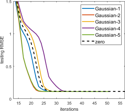
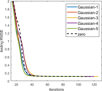
In this experiment, we study the following two initializations of $X$: (i) zero initialization (i.e., $X_{1}=0$) as shown in Algorithms 2 and 4; and (ii) Gaussian initialization, in which elements of $X_{1}$ are independently sampled from the standard normal distribution. We randomly generate 5 Gaussian initializations. The other parameters are fixed at $m=2000$, $r=5$, $o=0.25$, $s=2$ and $\sigma=10$.

Figure 6(a) (resp. Figure 6(b)) shows convergence of testing RMSE versus the number of iterations in Algorithm 2 for SDP-RL($\ell_{1}$) (resp. number of iterations in Algorithm 4 for SDP-RL(MCP)). As can be seen, all initializations lead to similar testing RMSEs. Some initializations lead to faster convergence, but Gaussian initialization is not always better than zero initialization.

(a) Algorithm 2.

(b) Algorithm 4.

Figure 6: Convergence of testing RMSE versus different initializations for the proposed algorithms.

6.2 Robust NPKL

In this section, experiment is performed on the adult data set “a1a”, which has been commonly used in the NPKL literature [19]. It contains $\bar{n}=1605$ 123-dimensional samples. Following [70], we randomly sample $6\bar{n}$ pairs and construct set ${\mathcal{T}}=\{T_{ij}\}$, where $T_{ij}=1$ if samples $i$ and $j$ have the same label, and $T_{ij}=0$ otherwise. We then randomly sample $60\%$ of the pairs in ${\mathcal{T}}$ for training, $20\%$ for validation and hyper-parameter tuning, and the rest for testing. The numbers of must-link and cannot-link pairs in the training/validation/testing sets are shown in Table IX. The Laplacian $L$ in (29) is constructed from a graph $G$. Each node in $G$ corresponds to a training sample, and is connected to its two nearest training samples based on the distance in the feature space.

TABLE IX: Numbers of must-link and cannot-link pairs in the robust NPKL experiment.

	must-link	cannot-link
training	3637	2141
validation	1210	716
testing	1220	706

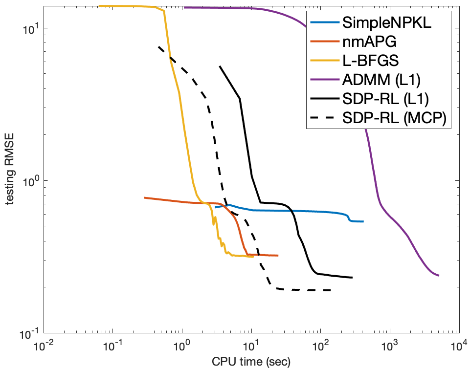
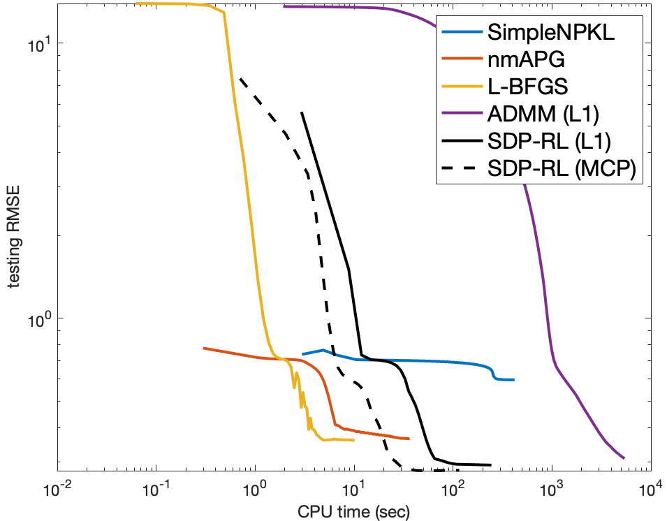
To test the robustness of NPKL algorithms, we flip some must-link constraints in the training set to cannot-link constraints, and vice versa. This mimics the label flipping attacks in real-world applications [39]. The total number of constraints flipped is varied in $\{5\%,10\%\}$.

Besides comparing with the previous methods based on the square loss, $\ell_{1}$ loss and leaky-MCP loss, we also compare with SimpleNPKL [19], which is based on the square loss but does not use the low-rank factorization. As for the rank $r$ of the initial solution $X$, we follow [21] and set its value to be the largest $r$ satisfying $\frac{r(r+1)}{2}\leq|{\mathcal{T}}|$. For performance evaluation, we follow [32, 41] and use the (i) testing root mean square error, $\text{RMSE}=(\sum\nolimits_{(i,j)\in{\mathcal{T}}_{\text{test}}}(Z_{ij}-T_{ij})^{2}/|{\mathcal{T}}_{\text{test}}|)^{1/2}$, where $\bar{X}$ is the output of the algorithm and ${\mathcal{T}}_{\text{test}}$ is the testing set, and (ii) CPU time.

(a) 5% flipped labels.

(b) 10% flipped labels.

Figure 7: Convergence of testing RMSE vs CPU time (sec) in the robust NPKL experiment.

TABLE X: Testing RMSEs and CPU time (sec) in the robust CMVU experiment.

loss	algorithm	small deviations		5% large outliers		10% large outliers
		testing RMSE	CPU time	testing RMSE	CPU time	testing RMSE	CPU time
square	SimpleCMVU	0.48$\pm$0.02	837$\pm$19	0.77$\pm$0.03	1675$\pm$49	0.97$\pm$0.03	1263$\pm$33
	nmAPG	0.34$\pm$0.01	342$\pm$5	0.65$\pm$0.04	691$\pm$15	0.76$\pm$0.01	280$\pm$2
	L-BFGS	0.34$\pm$0.01	424$\pm$7	0.46$\pm$0.01	645$\pm$15	0.58$\pm$0.01	574$\pm$2
$\ell_{1}$	ADMM($\ell_{1}$)	0.30$\pm$0.03	3090$\pm$27	0.34$\pm$0.03	2944$\pm$23	0.35$\pm$0.03	3124$\pm$29
	SDP-RL($\ell_{1}$)	0.29$\pm$0.02	165$\pm$23	0.32$\pm$0.03	113$\pm$50	0.33$\pm$0.02	113$\pm$33
leaky-MCP	SDP-RL(MCP)	0.25$\pm$0.02	206$\pm$38	0.29$\pm$0.02	156$\pm$53	0.30$\pm$0.03	162$\pm$40

(a) small deviations.

(b) 5% large outliers.

(c) 10% large outliers.

Figure 8: Convergence of testing RMSE vs CPU time (sec) in the robust CMVU experiment.

Table VII and Figure 7 show performance of the compared algorithms. As can be seen, algorithms based on the $\ell_{1}$ and non-convex losses have lower testing RMSE’s than those based on the square loss, with SDP-RL(MCP) being the best. Moreover, SDP-RL($\ell_{1}$) and SDP-RL(MCP) are faster than ADMM($\ell_{1}$).

6.3 Robust CMVU

In this section, we perform experiment on robust CMVU using the commonly-used USPS data set, which contains 2007 256-dimensional samples. As in [17], the set $\Omega$ in (31) is constructed by using the nearest $1\%$ neighbors of each sample, leading to $|\Omega|=401,400$. The squared Euclidean distance $t_{ij}$ for each $(i,j)\in\Omega$ is computed from the clean data set (before adding noise). We randomly sample $60\%$ of the pairs from $\Omega$ for training, $20\%$ for validation and hyper-parameter tuning, and the rest for testing. As for the rank $r$ of the initial solution $X$, we follow [21] and set its value to the largest $r$ satisfying $r(r+1)/2\leq|\Omega|$. The tradeoff parameter $\gamma$ in (31) is fixed at $0.01$.

For performance evaluation, we use (i) the testing RMSE: $(\sum\nolimits_{(i,j)\in\Omega_{\text{test}}}\big{(}Z_{ii}\!+\!Z_{jj}\!-\!2Z_{ij}\!-\!t_{ij}\big{)}^{2}/|\Omega_{\text{test}}|)^{\frac{1}{2}}$, where $\Omega_{\text{test}}$ is the testing portion of $\Omega$, and (ii) CPU time. Since NPKL and CMVU can be solved using the same algorithm, we use the same baselines as in Section 6.2, i.e. SimpleCMVU [19].

(a) $r=50$.

(b) $r=100$.

(c) $r=200$.

Figure 9: Percentage of explained variance vs CPU time (sec) for the various algorithms on the sparse PCA problem.

6.3.1 Small Gaussian Noise

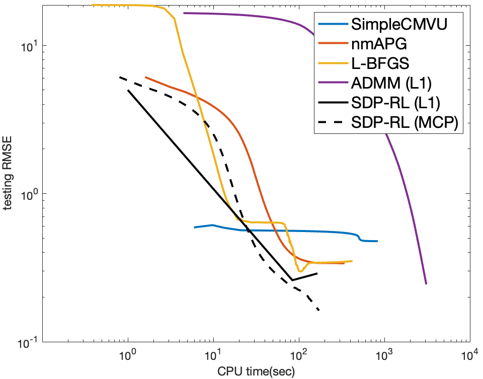
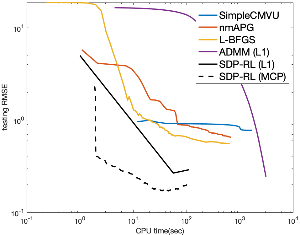
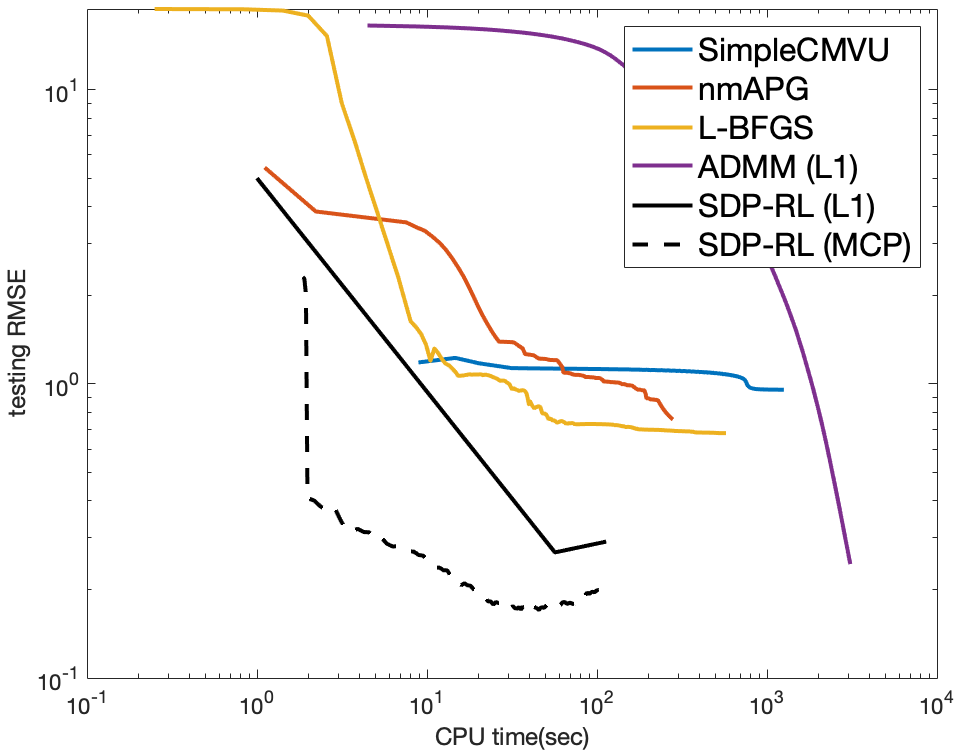
Here, we add Gaussian noise from $\mathcal{N}(0,0.01\cdot\text{Var}(x))$ to each feature in the training set, where $\text{Var}(x)$ is a vector containing the variance of each feature. Table X and Figure 8 show the results. The observations are almost the same as that in Section 6.2. SDP-RL(MCP) has the lowest testing RMSE, while ADMM($\ell_{1}$) and SDP-RL($\ell_{1}$) are better than nmAPG and L-BFGS. SDP-RL($\ell_{1}$) is also much more efficient than ADMM($\ell_{1}$).

6.3.2 Large Outliers

In this experiment, we add large outliers which may appear in the data [32, 41]. First, we randomly sample some samples ($5\%$ and $10\%$) from the training set. For each selected sample $x_{i}$, we add random noise from $\mathcal{N}(0,5\tilde{x})$, where $\tilde{x}$ is a vector containing the largest absolute feature value for that dimension. Table X and Figure 8 show the performance against outliers. Again, SDP-RL(MCP) has the lowest testing RMSE among the algorithms. Moroever, SDP-RL($\ell_{1}$) is much faster than ADMM($\ell_{1}$).

6.4 Sparse PCA

In this section, we perform sparse PCA experiment on the colon cancer data set [5], which contains $2000$ micro-array readings from $62$ subjects. We set $\lambda=0,\gamma=10$ in (33), and try different embedding dimensions $r=\{50$, $100$, $200\}$. As there are no missing data in sparse PCA, data sparsity is not utilized for SDP-RL. We also compare with two state-of-the-art sparse PCA methods:

1. nonlinear IPM [71], which obtains the sparse principal components from the following inverse eigenvalue problem: $\min_{x\in\mathbb{R}^{n}}\frac{(1-\alpha)\|x\|_{2}+\alpha\|x\|_{1}}{x^{\top}\Sigma x}$, where $\alpha$ is a hyper-parameter controlling the sparsity of $x$. When $\alpha=0$, it reduces to original PCA.

2. SpaSM [72], which solves the sparse PCA problem in (33) with the SPCA algorithm in [15].

For performance evaluation, as in [5, 13], we use the (i) CPU time, (ii) sparsity of $XX^{\top}$ (i.e., ratio of zero elements), and (iii) explained variance (i.e., $\text{tr}(Z\Sigma)$ in (32)). Experiments are repeated five times.

6.4.1 Results

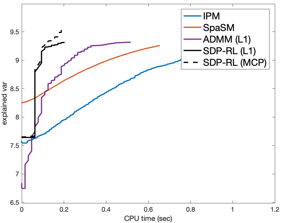
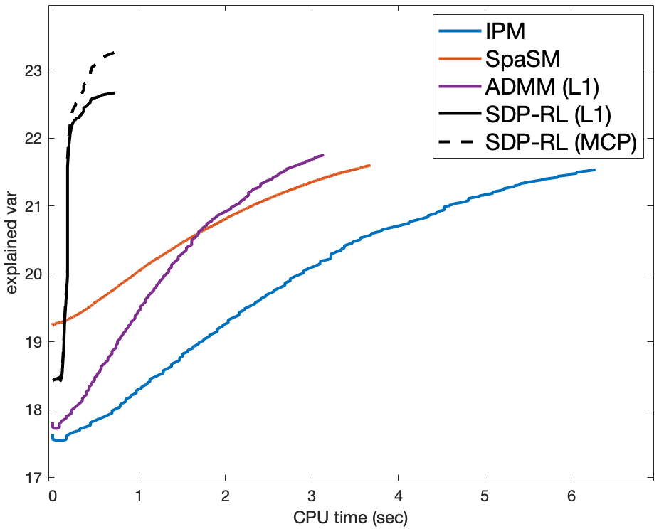
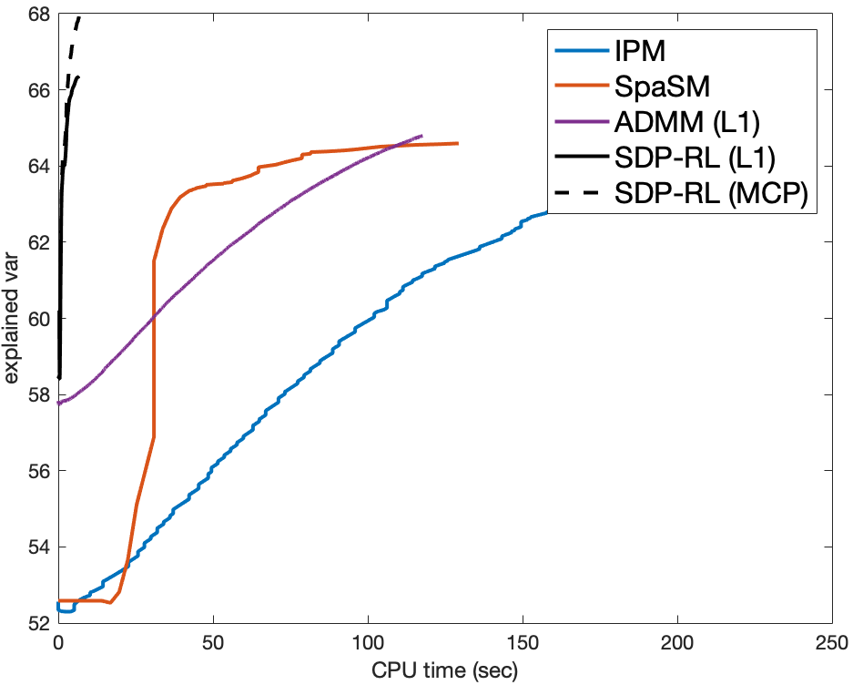
Results are shown in Table XI. As can been seen, due to the use of the non-convex loss, SDP-RL(MCP) produces the best solution compared with the other approaches. Besides, both SDP-RL($\ell_{1}$) and SDP-RL(MCP) are much faster than ADMM($\ell_{1}$), SpaSM and nonlinear IPM. Figure 9 shows convergence of the explained variance with CPU time. As can be seen, SDP-RL($\ell_{1}$) and SDP-RL(MCP) also converge much faster than the other approaches.

TABLE XI: Performance of various sparse PCA algorithms on the colon cancer data set.

$r$	algorithm	CPU time (sec)	sparsity	explained variance
50	nonlinear IPM	1.06$\pm$0.12	0.73	8.98
	SpaSM	0.64$\pm$0.03	0.63	8.92
	ADMM($\ell_{1}$)	0.55$\pm$0.06	0.76	9.23
	SDP-RL($\ell_{1}$)	0.21$\pm$0.02	0.76	9.23
	SDP-RL(MCP)	0.23$\pm$0.02	0.76	9.58
100	nonlinear IPM	6.18$\pm$0.36	0.75	21.83
	SpaSM	3.49$\pm$0.23	0.67	21.87
	ADMM($\ell_{1}$)	3.12$\pm$0.25	0.79	21.86
	SDP-RL($\ell_{1}$)	0.75$\pm$0.07	0.79	22.67
	SDP-RL(MCP)	0.86$\pm$0.12	0.79	23.22
200	nonlinear IPM	244.36$\pm$20.68	0.79	60.18
	SpaSM	120.94$\pm$8.26	0.75	62.74
	ADMM($\ell_{1}$)	118.28$\pm$12.25	0.82	64.24
	SDP-RL($\ell_{1}$)	7.42$\pm$0.23	0.82	66.44
	SDP-RL(MCP)	7.68$\pm$0.35	0.82	67.92

6.4.2 Effect of Different Initializations

In this experiment, we study the following two initializations of $X$: (i) zero initialization as in Algorithm 2 and 4; and (ii) standard PCA. Results are shown in Table XII. As can be seen, different initializations have little impact on the final performance, but initialization by PCA can have faster convergence. This also agrees with the common practice of using PCA as initialization for sparse PCA [15].

TABLE XII: Effect of different ways to initialize SDP-RL in the sparse PCA experiment.

$r$	loss in SDP-RL	initialization	CPU time (sec)	sparsity	explained variance
50	$\ell_{1}$	zero	0.21$\pm$0.02	0.76	9.23
		PCA	0.11$\pm$0.01	0.75	9.26
	MCP	zero	0.23$\pm$0.02	0.76	9.58
		PCA	0.11$\pm$0.02	0.78	9.57
100	$\ell_{1}$	zero	0.75$\pm$0.07	0.79	22.67
		PCA	0.29$\pm$0.04	0.80	22.78
	MCP	zero	0.86$\pm$0.12	0.79	23.22
		PCA	0.35$\pm$0.07	0.79	23.24
200	$\ell_{1}$	zero	7.42$\pm$0.23	0.82	66.44
		PCA	4.14$\pm$0.19	0.81	66.48
	MCP	zero	7.68$\pm$0.35	0.82	67.92
		PCA	4.35$\pm$0.23	0.82	68.03

As can be seen from experiments in both Section 6.1.6 and here, the choice of initialization is application-specific. Empirically, different initializations have little impact on the final performance of the proposed algorithm, but a better initialization can lead to faster convergence.

6.5 Symmetric NMF

In this section, we perform experiments on symmetric nonnegative matrix factorization (SNMF). Data generation is similar to that in Section 6.1, with the ground-truth matrix $M$ generated as $VV^{\top}$. In the first experiment, $V\in\mathbb{R}^{m\times 5}$ is synthetic, with $m\in\{1000,2000\}$. Each element of $V$ is sampled independently from the standard exponential distribution. We then corrupt $M$ by adding a sparse matrix $S$, which models a fraction of $o$ large outliers sampled uniformly from $\{0,\sigma\}$, to obtain $M^{\prime}=M+S$. The training/validation/test set split follows that in Section 6.1. The second experiment is similar, except that $V$ is constructed from real-world data set. Specifically, following [68], we construct $V\in\mathbb{R}^{2007\times 10}$ as the one-hot label matrix for the USPS dataset in Section 6.3.

The rank $r$ of the initial $X$ solution is set to the ground-truth, i.e. $5$ for the esynthetic data and $10$ for USPS dataset. The other parameters are set as $o=0.05$, $s=2$ and $\sigma=10$.

We compare SDP-RL with three commonly-used SNMF methods [68, 67]: Newton’s method (Newton) [66], regularized eigenvalue decomposition (rEVD) [73], and block-coordinate descent (BCD) [67]. All three solve (34) (with the square loss) while the proposed SDP-RL solves problem (35) (with the $\ell_{1}$-loss). For performance evaluation, we follow Section 6.1 and use the testing RMSE and CPU time.

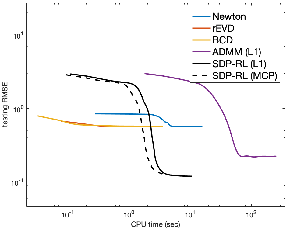
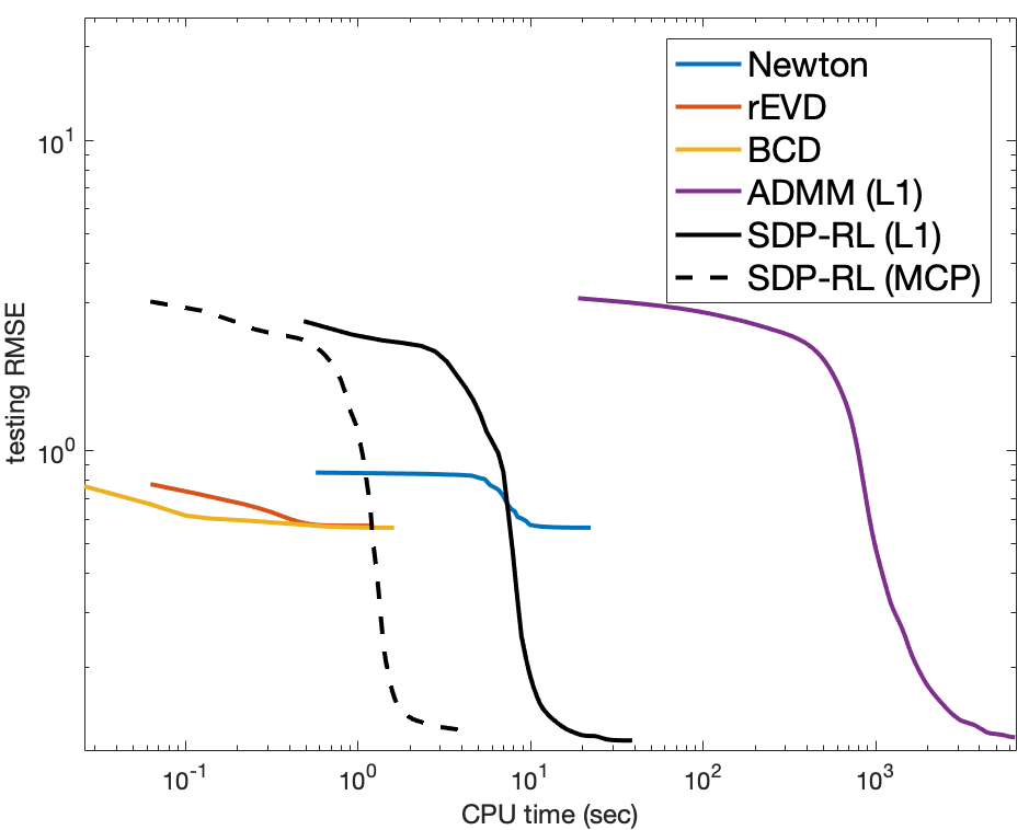
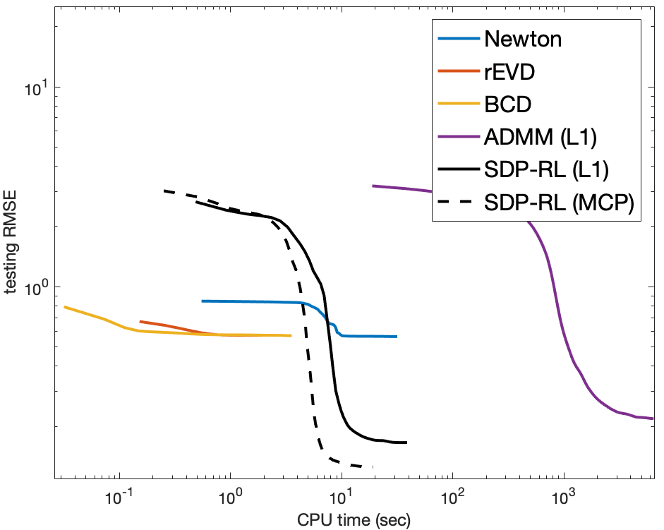
Results are shown in Table XIII, and the convergence of testing RMSE w.r.t. CPU time is shown in Figure 10. Again, they demonstrate that SDP-RL (using either the $\ell_{1}$ or MCP loss) is significantly more robust (lower testing RMSE) on noisy data as compared to methods based on the square loss. Moreover, SDP-RL($\ell_{1}$) is more efficient than ADMM($\ell_{1}$).

TABLE XIII: Testing RMSEs and CPU time (sec) in the SNMF experiment.

loss	algorithm	synthetic ($m=1000$)		synthetic ($m=2000$)		USPS
		testing RMSE	CPU time	testing RMSE	CPU time	testing RMSE	CPU time
square	Newton	0.783$\pm$0.007	9$\pm$1	0.564$\pm$0.003	22$\pm$6	0.821$\pm$0.006	25$\pm$7
	rEVD	0.799$\pm$0.005	0.5$\pm$0.1	0.571$\pm$0.002	1.2$\pm$0.2	0.832$\pm$0.007	2.0$\pm$0.4
	BCD	0.781$\pm$0.008	1.6$\pm$0.5	0.565$\pm$0.003	2.9$\pm$0.8	0.823$\pm$0.009	3.2$\pm$0.6
$\ell_{1}$	ADMM($\ell_{1}$)	0.433$\pm$0.006	515$\pm$27	0.330$\pm$0.005	2763$\pm$47	0.486$\pm$0.007	3018$\pm$65
	SDP-RL($\ell_{1}$)	0.212$\pm$0.004	12$\pm$1	0.158$\pm$0.002	35$\pm$2	0.267$\pm$0.009	39$\pm$4
leaky-MCP	SDP-RL(MCP)	0.119$\pm$0.002	15$\pm$3	0.112$\pm$0.001	48$\pm$4	0.194$\pm$0.006	57$\pm$8

(a) synthetic ($m=1000$).

(b) synthetic ($m=2000$).

(c) USPS.

Figure 10: Convergence of testing RMSE vs CPU time (sec) in the SNMF experiment.

7 Conclusion

In this paper, we propose a robust and factorized formulation of SDP by replacing the commonly used square loss with more robust losses ($\ell_{1}$-loss and non-convex losses). As the resulting optimization problem is neither convex nor smooth, existing SDP solvers cannot be applied. We propose a new solver based on majorization-minimization. By allowing inexactness in the underlying ADMM subproblem, the algorithm is much more efficient while still guaranteed to converge to a critical point. Experiments are performed on five applications: matrix completion, kernel learning, matrix variance unfolding, sparse PCA, and symmetric non-negative matrix factorization. Empirical results demonstrate the efficiency and robustness over state-of-the-arts SDP solvers.

8 Acknowledgment

This research was supported in part by the National Natural Science Foundation of China (No.61663049).

Quanming Yao (member, IEEE) is currently a senior scientist in 4Paradigm (Hong Kong) and an incoming assistant professor (tenure-track) of Department of Electrical Engineering Tsinghua University. His research interests are in machine learning, nonconvex optimization, and automated machine learning. He obtained his Ph.D. degree in the Department of Computer Science and Engineering at Hong Kong University of Science and Technology (HKUST) in 2018. He has received Wunwen Jun Prize for Excellence Youth of Artificial Intelligence (issued by CAAI, 2019), the 1st runner up of Ph.D. Research Excellence Award (School of Engineering, HKUST, 2018-2019) and Google Fellowship (machine learning, 2016).

Hansi Yang joins Tsinghua University in 2017, and is an undergraduate student with Department of Electronic Engineering. He is currently an intern in machine learning research group of 4Paradigm Inc supervised by Dr. Yao. His research interests are in machine learning and automated machine learning.

En-Liang Hu (member, IEEE) En-Liang Hu received his Ph.D. degree in computer science from the Nanjing University of Aeronautics and Astronautics, Nanjing, China, in 2010. He is currently a Professor with the Department of Mathematics, Yunnan Normal University, Cheng Gong Campus, Kunming. His current research interests include machine learning, data mining, and optimization.

James T. Kwok (Fellow, IEEE) received the Ph.D. degree in computer science from The Hong Kong University of Science and Technology in 1996. He is a Professor with the Department of Computer Science and Engineering, Hong Kong University of Science and Technology. His research interests include machine learning, deep learning, and artificial intelligence. He received the IEEE Outstanding 2004 Paper Award and the Second Class Award in Natural Sciences by the Ministry of Education, China, in 2008. He is serving as an Associate Editor for the IEEE Transactions on Neural Networks and Learning Systems, Neural Networks, Neurocomputing, Artificial Intelligence Journal, International Journal of Data Science and Analytics, Editorial Board Member of Machine Learning, Board Member, and Vice President for Publications of the Asia Pacific Neural Network Society. He also served/is serving as Senior Area Chairs / Area Chairs of major machine learning / AI conferences including NIPS, ICML, ICLR, IJCAI, AAAI and ECML.

Appendix A Proof

A.1 Lemma 1

Proof.

First, we have

$$\lvert\text{tr}\big{(}(X_{k}+{\tilde{X}}){{}^{\top}}Q_{\tau}(X_{k}+{\tilde{X}})\big{)}-t_{\tau}\rvert$$

$$=\lvert\text{tr}(2{\tilde{X}}{{}^{\top}}Q_{\tau}X_{k}+X_{k}^{\top}Q_{\tau}X_{k})-t_{\tau}+\text{tr}({\tilde{X}}{{}^{\top}}Q_{\tau}{\tilde{X}})\rvert,$$

$$\leq\lvert\text{tr}(2{\tilde{X}}{{}^{\top}}Q_{\tau}X_{k}+X_{k}^{\top}Q_{\tau}X_{k})-t_{\tau}\rvert+\lvert\text{tr}({\tilde{X}}{{}^{\top}}Q_{\tau}{\tilde{X}})\rvert.\!\!\!$$ (36)

Then, let $C=A+\frac{\lambda}{\gamma}I$, we have,

$$\frac{\gamma}{2}\text{tr}\big{(}(X_{k}+{\tilde{X}}){{}^{\top}}A(X_{k}+{\tilde{X}})\big{)}+\frac{\lambda}{2}\text{tr}\big{(}(X_{k}+{\tilde{X}}){{}^{\top}}(X_{k}+{\tilde{X}})\big{)}$$

$$=\frac{\gamma}{2}\text{tr}\big{(}{\tilde{X}}^{{}^{\top}}C{\tilde{X}}+(X_{k}+2{\tilde{X}})^{\top}CX_{k}\big{)}.$$ (37)

Recall that

$$R({\tilde{X}} +X_{k})=\sum\nolimits_{\tau=1}^{m}\lvert\text{tr}(({\tilde{X}}+X_{k})^{\top}Q_{\tau}({\tilde{X}}+X_{k}))-t_{\tau}\rvert$$

$$+ \frac{\gamma}{2}\text{tr}(({\tilde{X}}+X_{k})^{\top}A({\tilde{X}}+X_{k}))+\frac{\lambda}{2}\|{\tilde{X}}+X_{k}\|_{F}^{2}.$$

Combining (36), (37) and the definition of $R({\tilde{X}}+X_{k})$ above, thus for any $\tilde{X}\in{\mathbb{R}}^{n\times r}$ we have

$$R({\tilde{X}}+X_{k})\leq\sum\nolimits_{\tau=1}^{m}\lvert\text{tr}(2{\tilde{X}}{{}^{\top}}Q_{\tau}X_{k}+X_{k}^{\top}Q_{\tau}X_{k})-t_{\tau}\rvert$$

$$+\sum\nolimits_{\tau=1}^{m}\lvert\text{tr}({\tilde{X}}{{}^{\top}}Q_{\tau}{\tilde{X}})\rvert+\frac{\gamma}{2}\text{tr}\big{(}{\tilde{X}}^{{}^{\top}}C{\tilde{X}}+(X_{k}+2{\tilde{X}})^{\top}CX_{k}\big{)}.$$

Thus, we obtain the Lemma. ∎

A.2 Lemma 2

Proof.

Since we have $\text{tr}({\tilde{X}}{{}^{\top}}Q_{\tau}{\tilde{X}})=\text{tr}({\tilde{X}}{{}^{\top}}\frac{1}{2}(Q_{\tau}+Q_{\tau}^{\top}){\tilde{X}})$ and $\frac{1}{2}(Q_{\tau}+Q_{\tau}^{\top})$ is always symmetric for any $Q_{\tau}\in\mathbb{S}^{+}$, we only need to prove that: let $\bar{S}=S_{+}-S_{-}$ where $S\in\mathbb{S}^{n}$ is any symmetric matrix, then $|\text{tr}({\tilde{X}}{{}^{\top}}S{\tilde{X}})|\leq\text{tr}({\tilde{X}}{{}^{\top}}\bar{S}{\tilde{X}})$ holds for every $\tilde{X}\in{\mathbb{R}}^{n\times r}$. Let $\lambda_{\max}=\sum\nolimits_{i=1}^{n}\max(\lambda_{i},0)v_{i}v_{i}^{\top}$ and $\lambda_{\min}=\sum\nolimits_{i=1}^{n}\min(\lambda_{i},0)v_{i}v_{i}^{\top}$. Thus, we have

$$|\text{tr}({\tilde{X}}{{}^{\top}}S{\tilde{X}})| =|\text{tr}({\tilde{X}}{{}^{\top}}(\sum\nolimits_{i=1}^{n}\lambda_{i}v_{i}v_{i}^{\top}){\tilde{X}})|,$$

$$\leq|\text{tr}({\tilde{X}}{{}^{\top}}\lambda_{\max}{\tilde{X}})|+|\text{tr}({\tilde{X}}{{}^{\top}}\lambda_{\min}{\tilde{X}})|,$$

$$=\text{tr}({\tilde{X}}{{}^{\top}}\lambda_{\max}{\tilde{X}})-\text{tr}({\tilde{X}}{{}^{\top}}\lambda_{\min}{\tilde{X}}),$$

$$=\text{tr}({\tilde{X}}{{}^{\top}}S_{+}{\tilde{X}})-\text{tr}({\tilde{X}}{{}^{\top}}S_{-}{\tilde{X}})=\text{tr}({\tilde{X}}{{}^{\top}}\bar{S}{\tilde{X}}).$$

Thus, we obtain the Lemma. ∎

A.3 Proposition 2

Proof.

Combining Lemma 1 and 2 we will have,

$$R({\tilde{X}}+X_{k})\leq\sum\nolimits_{\tau=1}^{m}\lvert\text{tr}(2{\tilde{X}}{{}^{\top}}Q_{\tau}X_{k}+X_{k}^{\top}Q_{\tau}X_{k})-t_{\tau}\rvert$$

$$+\sum\nolimits_{\tau=1}^{m}\lvert\text{tr}({\tilde{X}}{{}^{\top}}Q_{\tau}{\tilde{X}})\rvert+\frac{\gamma}{2}\text{tr}\big{(}{\tilde{X}}^{{}^{\top}}C{\tilde{X}}+(X_{k}+2{\tilde{X}})^{\top}CX_{k}\big{)},$$

$$\leq 2\sum\nolimits_{\tau=1}^{m}\lvert\text{tr}({\tilde{X}}{{}^{\top}}Q_{\tau}X_{k})+\frac{1}{2}(\text{tr}(X_{k}^{\top}Q_{\tau}X_{k})-t_{\tau})\rvert$$

$$+\sum\nolimits_{\tau=1}^{m}\text{tr}({\tilde{X}}{{}^{\top}}\bar{Q}_{\tau}{\tilde{X}})+\frac{\gamma}{2}\text{tr}\big{(}{\tilde{X}}^{{}^{\top}}C{\tilde{X}}+(X_{k}+2{\tilde{X}})^{\top}CX_{k}\big{)},$$

Then, let $B=Q+\frac{1}{2}(\lambda I+\gamma A_{+})$, $Q=\sum\nolimits_{\tau=1}^{m}\bar{Q}_{\tau}$, $(b_{k})_{\tau}=\frac{1}{2}(\text{tr}(X_{k}{{}^{\top}}Q_{\tau}X_{k})-t_{\tau})$, and $c_{k}=\frac{\gamma}{2}\text{tr}(X_{k}{{}^{\top}}(A+\frac{\lambda}{\gamma}I)X_{k})$,

$$R({\tilde{X}}+X_{k})\leq 2\sum\nolimits_{\tau=1}^{m}\lvert\text{tr}({\tilde{X}}{{}^{\top}}Q_{\tau}X_{k})+(b_{k})_{\tau}\rvert$$

$$+\text{tr}({\tilde{X}}{{}^{\top}}(B{\tilde{X}}+\gamma CX_{k}))+c_{k},$$

then $R({\tilde{X}}+X_{k})\leq H_{k}({\tilde{X}};X_{k})$ where

$$H_{k}({\tilde{X}};X_{k})= \text{tr}({\tilde{X}}{{}^{\top}}(B{\tilde{X}}+\gamma CX_{k}))$$

$$+2\sum\nolimits_{\tau=1}^{m}\lvert\text{tr}({\tilde{X}}{{}^{\top}}Q_{\tau}X_{k})+(b_{k})_{\tau}\rvert+c_{k},$$

and the equality holds iff $\tilde{X}=\mathbf{0}$. ∎

A.4 Proposition 3

Proof.

Following its definition, denote the dual problem to be $\max_{\{\tilde{\nu}_{\tau}\}}\mathcal{D}_{k}(\{\tilde{\nu}_{\tau}\})$, which is defined as:

$$\mathcal{D}_{k}(\{\tilde{\nu}_{\tau}\})= \min_{{\tilde{X}},e_{\tau}}\text{tr}({\tilde{X}}{{}^{\top}}(B{\tilde{X}}+\gamma CX_{k}))+2\sum\nolimits_{\tau=1}^{m}\lvert e_{\tau}\rvert+c_{k},$$

$$+\sum\nolimits_{\tau=1}^{m}\tilde{\nu}_{\tau}(\text{tr}({\tilde{X}}{{}^{\top}}Q_{\tau}X_{k})+(b_{k})_{\tau}-e_{\tau}).$$

The problem above can be solved by minimizing w.r.t. ${\tilde{X}}$ and $e_{\tau}$ separately. We first consider minimizing w.r.t. $e_{\tau}$, which is given by $\min_{e_{\tau}}2\sum\nolimits_{\tau=1}^{m}\lvert e_{\tau}\rvert-\sum\nolimits_{\tau=1}^{m}\tilde{\nu}_{\tau}e_{\tau}$ and it follows easily that when $|\tilde{\nu}_{\tau}|>2$, the problem above achieves $-\inf$. So it requires $|\tilde{\nu}_{\tau}|\leq 2$ and the minimized point is 0. We then turned on to consider minimizing w.r.t. ${\tilde{X}}$, which is (we omit the $c_{k}$ term for simplicity, as it has no influence to the optimization problem)

$$\min_{{\tilde{X}}}\text{tr}({\tilde{X}}{{}^{\top}}(B{\tilde{X}}\!+\!\gamma CX_{k}))\!+\!\sum_{\tau=1}^{m}\tilde{\nu}_{\tau}(\text{tr}({\tilde{X}}{{}^{\top}}Q_{\tau}X_{k})\!+\!(b_{k})_{\tau}),$$

$$\!\!\!=\!\min_{{\tilde{X}}}\text{tr}({\tilde{X}}{{}^{\top}}(B{\tilde{X}}\!+\!(\gamma C\!+\!\!\sum_{\tau=1}^{m}\tilde{\nu}_{\tau}Q_{\tau})X_{k}))\!+\!\!\sum_{\tau=1}^{m}\tilde{\nu}_{\tau}(b_{k})_{\tau}.\!\!\!$$ (38)

Let $D=\gamma C+\sum\nolimits_{\tau=1}^{m}\tilde{\nu}_{\tau}Q_{\tau}$, (38) is equivalent to

$$\min_{{\tilde{X}}}\sum\nolimits_{\tau=1}^{m}\tilde{\nu}_{\tau}(b_{k})_{\tau}-\frac{1}{4}\text{tr}(D^{\top}B^{-1}D).$$

Thus, the optimal of (38) is

$${\tilde{X}}^{*}=-\frac{1}{2}B^{-1}D.$$

Then, the dual problem is $\max_{|\tilde{\nu}_{\tau}|\leq 2}\mathcal{D}_{k}(\{\tilde{\nu}_{\tau}\})$ where $\mathcal{D}_{k}$ is defined in Proposition 3. ∎

A.5 Lemma 3

Proof.

Specifically, since our problem in (3.1.2) is convex (convex objective and linear constraints), we only need to check the Slater’s condition, i.e. there exists a strictly feasible point for this problem, in order to prove its strong duality. And the proof is trivial as we have $\tilde{X}\in\mathbb{R}^{n\times r},\{e_{\tau}\in\mathbb{R}\}$, therefore the constraints $e_{\tau}=\text{tr}(\tilde{X}^{\top}Q_{\tau}X_{k})+(b_{k})_{\tau}$ can always be satisfied by choosing an appropriate $e_{\tau}$. ∎

A.6 Theorem 1

We first introduce the following Lemma 5 and 6. When a function $f$ has multiple input parameters, $\partial_{k}f$ means taking subdifferential to its $k$th parameter.

Lemma 5.

There exists a positive constant $\alpha>0$, such that

1. $H_{k}({\tilde{X}}_{1};X_{k})\geq H_{k}({\tilde{X}}_{2};X_{k})+\frac{\alpha}{2}\|{\tilde{X}}_{1}-{\tilde{X}}_{2}\|_{F}^{2}$ holds for any ${\tilde{X}}_{1},{\tilde{X}}_{2}$; and

2. $R(X_{k})-R(X_{k+1})\geq\frac{\alpha}{2}\|X_{k+1}-X_{k}\|^{2}-\epsilon_{k}$.

Proof.

Part 1). Recall from (14) in Proposition 2 that $H_{k}$ is defined as

$$H_{k}({\tilde{X}};X_{k}) \equiv\text{tr}({\tilde{X}}{{}^{\top}}(B{\tilde{X}}+\gamma CX_{k}))$$

$$+2\sum\nolimits_{\tau=1}^{m}\lvert\text{tr}({\tilde{X}}{{}^{\top}}Q_{\tau}X_{k})+(b_{k})_{\tau}\rvert+c_{k}.$$ (39)

Thus, to show Part 1) holds, we only need to show that the smallest eigenvalue of $B$ in the quadratic term, i.e., the first term in $H_{k}$, is positive. This can be easily seen from the definition of $B$, i.e., $B=\sum\nolimits_{\tau=1}^{m}\bar{Q}_{\tau}+\frac{1}{2}(\lambda I+\gamma A_{+})$, since $A_{+}$, $\bar{Q}_{\tau}$ are PSD from its definition and Lemma 2, $I$ is the identity matrix, and $\lambda$ is required to be positive.

Part 2). From Proposition 2, we know

$$R(X_{k}) =H_{k}(\bm{0},X_{k}),$$ (40)

$$R(X_{k}+{\tilde{X}}^{*}) \leq H_{k}({\tilde{X}}^{*},X_{k}).$$ (41)

Recall that ${\tilde{X}}^{*}$ is approximated by ${\tilde{X}}_{t}$ in step 3 of Algorithm 2. Using (40) and (41), we have

$$R(X_{k})-R(X_{k}+{\tilde{X}}^{*})\geq H_{k}(\bm{0},X_{k})-H_{k}({\tilde{X}}^{*},X_{k}),$$

$$=\big{[}H_{k}(\bm{0},X_{k})-H_{k}({\tilde{X}}_{t},X_{k})\big{]}$$

$$\qquad\qquad+\big{[}H_{k}({\tilde{X}}_{t},X_{k})-H_{k}({\tilde{X}}^{*},X_{k})\big{]}.$$ (42)

Using $\delta_{k}$’s definition in (21), we have

$$\epsilon_{k}\geq\delta_{k}({\tilde{X}}_{t},\{(\tilde{\nu}_{\tau})_{t}\}) =H_{k}({\tilde{X}}_{t};X_{k})-\mathcal{D}_{k}(\{\nu_{\tau}\}_{t}),$$

$$\geq H_{k}({\tilde{X}}_{t};X_{k})-H_{k}({\tilde{X}}^{*};X_{k}).$$

Thus,

$$-\epsilon_{k}\leq H_{k}({\tilde{X}}_{t},X_{k})-H_{k}({\tilde{X}}^{*},X_{k})\leq 0.$$ (43)

From part 1), we also have

$$H_{k}(\bm{0},X_{k}) -H_{k}({\tilde{X}}^{*},X_{k})$$

$$\geq\frac{\alpha}{2}\|X_{k+1}-X_{k}\|^{2}=\frac{\alpha}{2}\|{\tilde{X}}^{*}\|^{2}.$$ (44)

Finally, combining (42)-(44), we then obtain

$$R(X_{k})-R(X_{k+1})\geq\frac{\alpha}{2}\|X_{k+1}-X_{k}\|^{2}-\epsilon_{k}.$$

Thus, part 2) holds. ∎

Lemma 6.

1. $\partial_{2}H_{k}(\bm{0},X_{k})=\partial R(X_{k})$; and

2. $\bm{0}\in\lim\nolimits_{t\rightarrow\infty}\partial_{2}H_{k}({\tilde{X}}_{t},X_{k})$.

Proof.

Part 1). Recall the definition of $R(X)$ in (13), i.e.,

$$R({\tilde{X}} +X_{k})=\sum\nolimits_{\tau=1}^{m}\lvert\text{tr}(({\tilde{X}}+X_{k})^{\top}Q_{\tau}({\tilde{X}}+X_{k}))-t_{\tau}\rvert$$

$$+ \frac{\gamma}{2}\text{tr}(({\tilde{X}}+X_{k})^{\top}A({\tilde{X}}+X_{k}))+\frac{\lambda}{2}\|{\tilde{X}}+X_{k}\|_{F}^{2}.$$

Thus,

$$\partial R(X_{k})=\gamma AX_{k}+\lambda X_{k}+$$

$$+\sum\nolimits_{\tau=1}^{m}\text{sign}(\text{tr}(X_{k}^{\top}Q_{\tau}X_{k})-t_{\tau})\frac{1}{2}(Q_{\tau}+Q^{\top}_{\tau})X_{k}.$$ (45)

Then, recall the definition of $H_{k}$ in (39), we have

$$\partial_{2}H_{k}(\bm{0},X_{k}) =\gamma CX_{k}$$

$$+ 2\sum\nolimits_{\tau=1}^{m}\text{sign}\big{(}(b_{k})_{\tau}\big{)}\frac{1}{2}(Q_{\tau}+Q^{\top}_{\tau})X_{k}.$$ (46)

Since $C=A+\frac{\lambda}{\gamma}I$ and $(b_{k})_{\tau}=\frac{1}{2}(\text{tr}(X_{k}{{}^{\top}}Q_{\tau}X_{k})-t_{\tau})$ (defined in Proposition 2), we can deduce that the Lemma holds by comparing (45) and (46).

Part 2). Recall that ${\tilde{X}}_{t}=X_{k+1}-X_{k}$ is defined at step 3 of Algorithm 2. Using $\delta_{k}$’s definition in (21), we have

$$\delta_{k}({\tilde{X}}_{t},\{(\tilde{\nu}_{\tau})_{t}\}) =H_{k}({\tilde{X}}_{t};X_{k})-\mathcal{D}_{k}(\{\nu_{\tau}\}_{t}),$$

$$\geq H_{k}({\tilde{X}}_{t};X_{k})-H_{k}({\tilde{X}}^{*};X_{k})\geq 0.$$

Since $H_{k}$ is a continuous function and

$$\lim\nolimits_{t\rightarrow\infty}\delta_{k}({\tilde{X}}_{t},\{(\tilde{\nu}_{\tau})_{t}\})=0,$$

we have

$$\lim\nolimits_{t\rightarrow\infty}H_{k}({\tilde{X}}_{t};X_{k})-H_{k}({\tilde{X}}^{*};X_{k})=0,$$

which means $\bm{0}\in\lim\nolimits_{t\rightarrow\infty}\partial_{2}H_{k}({\tilde{X}}_{t},X_{k})$. ∎

Proof.

(of Theorem 1) Conclusion (i). From part 2) in Lemma 5, we have

$$\frac{\alpha}{2}\|X_{k+1}-X_{k}\|^{2}\leq R(X_{k})-R(X_{k+1})+\epsilon_{k}.$$

Thus,

$$\sum\nolimits_{k=1}^{K} \frac{\alpha}{2}\|X_{k+1}-X_{k}\|_{F}^{2}$$

$$\leq\sum\nolimits_{k=1}^{K}R(X_{k})-R(X_{k+1})+\epsilon_{k}$$

$$\leq R(X_{1})-R(X_{K+1})+\sum\nolimits_{k=1}^{K}\epsilon_{k}$$

$$\leq R(X_{1})-\inf R+\sum\nolimits_{k=1}^{\infty}\epsilon_{k}.$$ (47)

From Assumption 2, we know that the last term in (47), i.e., $\sum\nolimits_{k=1}^{\infty}\epsilon_{k}$, is finite. Together with Assumption 1, we have

$$\lim\nolimits_{k\rightarrow\infty} \|X_{k+1}-X_{k}\|_{F}^{2}=0,$$ (48)

  and $$0\leq\lim\nolimits_{k\rightarrow\infty}\|X_{k}\|_{F}^{2}<\infty,$$

which means that the sequence $\{X_{k}\}$ is bounded and has at least one limit points.

Conclusion (ii). From Part 1) in Lemma 6, we have $\partial_{2}H_{k}(\bm{0},X_{k})=\partial R(X_{k})$. Then, denote the limit point of sequence $\{X_{k}\}$ as $X_{*}$, and let $\{X_{k_{j}}\}$ be a sub-sequence of $\{X_{k}\}$ such that

$$X_{*}=\lim\nolimits_{k_{j}\rightarrow\infty}X_{k_{j}}.$$ (49)

Thus, to prove the limit point $X_{*}$ is also a critical point for $R(X)$, we only need to show

$$\bm{0}\in\lim\nolimits_{k_{j}\rightarrow\infty}\partial_{2}H_{k_{j}}(\bm{0},X_{*}).$$ (50)

Using Part 2) in Lemma 6, we should have

$$\bm{0} \in\lim\nolimits_{t\rightarrow\infty}\partial_{2}H_{k_{j}}({\tilde{X}}^{k_{j}}_{t},X_{k_{j}}),$$

$$=\partial_{2}H_{k_{j}}(\lim\nolimits_{t\rightarrow\infty}{\tilde{X}}^{k_{j}}_{t},X_{k_{j}}).$$ (51)

Thus, denote $\lim\nolimits_{t\rightarrow\infty}{\tilde{X}}^{k_{j}}_{t}={\tilde{X}}^{k_{j}}_{*}$, we only need to prove

$$\lim\nolimits_{k_{j}\to\infty}{\tilde{X}}^{k_{j}}_{*}=\bm{0}.$$ (52)

Since $\sum\nolimits_{k=1}^{\infty}\epsilon_{k}$ is finite, we must have $\lim\nolimits_{k_{j}\to\infty}\epsilon_{k_{j}}=0$, which implies that

$$\lim\nolimits_{k_{j}\rightarrow\infty}(X_{k_{j}+1}-X_{k_{j}}-{\tilde{X}}^{k_{j}}_{*})=\mathbf{0}.$$ (53)

Then from (48), we have

$$\lim\nolimits_{k_{j}\rightarrow\infty}X_{k_{j}+1}-X_{k_{j}}=\bm{0},$$ (54)

Then, (52) follows easily from (53) and (54). Finally, (50) can be obtained by combining (51) and (52). Thus, any limit point of $\{X_{k}\}$ is a critical point of $R$. ∎

A.7 Lemma 4

Proof.

Since $\phi(\cdot)$ is concave on $(0,\infty)$, we have $\phi(y)\leq\phi(x)+\phi^{\prime}(x)(y-x)$ for any $x,y\in(0,\infty)$. That means for any $\alpha,\beta\in\mathbb{R}$, $\phi(\lvert\beta\rvert)\leq\phi(\lvert\alpha\rvert)+\phi^{\prime}(\lvert\alpha\rvert)(\lvert\beta\rvert-\lvert\alpha\rvert)$. Then, we consider our objective:

$$R(X_{k}+\widetilde{X}) \!=\!\sum\nolimits_{\tau=1}^{m}\phi(|\text{tr}((X_{k}+\widetilde{X})^{\top}Q_{\tau}(X_{k}+\widetilde{X}))-t_{\tau}|),$$

$$\!+\!\frac{\gamma}{2}\text{tr}((X_{k}+\widetilde{X})^{\top}A(X_{k}+\widetilde{X}))+\frac{\lambda}{2}\|X_{k}+\widetilde{X}\|_{F}^{2},$$

$$\!=\!\sum\nolimits_{\tau=1}^{m}\phi(|\text{tr}((X_{k}+\widetilde{X})^{\top}Q_{\tau}(X_{k}+\widetilde{X}))-t_{\tau}|),$$

$$\!+\!\frac{\gamma}{2}\text{tr}(X_{k}^{\top}CX_{k})+\frac{\gamma}{2}\text{tr}((2X_{k}+\tilde{X})^{\top}C\tilde{X}),$$

where $C=A+\frac{\lambda}{\gamma}I$. Denote $(q_{k})_{\tau}=\phi^{\prime}\big{(}|\text{tr}(X_{k}^{\top}Q_{\tau}X_{k})-t_{\tau}|\big{)}$, we will have

$$\phi(|\text{tr}((X_{k}+\widetilde{X})^{\top}Q_{\tau}(X_{k}+\widetilde{X}))-t_{\tau}|)$$

$$\leq(q_{k})_{\tau}|\text{tr}((X_{k}+\widetilde{X})^{\top}Q_{\tau}(X_{k}+\widetilde{X}))-t_{\tau}|$$

$$+\big{(}\phi(|\text{tr}(X_{k}^{\top}Q_{\tau}X_{k})-t_{\tau}|)-(q_{k})_{\tau}|\text{tr}(X_{k}^{\top}Q_{\tau}X_{k})-t_{\tau}|\big{)}$$

And it follows easily that:

$$|\text{tr}((X_{k}+\widetilde{X})^{\top}Q_{\tau}(X_{k}+\widetilde{X}))-t_{\tau}|$$

$$\leq|\text{tr}((2\tilde{X}+X_{k})^{\top}Q_{\tau}X_{k})-t_{\tau}|+|\text{tr}(\tilde{X}^{\top}Q_{\tau}\tilde{X})|$$

Denote

$$\dot{c}_{k} =\sum\nolimits_{\tau=1}^{m}\big{(}\phi(|\text{tr}(X_{k}^{\top}Q_{\tau}X_{k})$$

$$-t_{\tau}|)-(q_{k})_{\tau}|\text{tr}(X_{k}^{\top}Q_{\tau}X_{k})-t_{\tau}|\big{)}+\frac{\gamma}{2}\text{tr}(X_{k}^{\top}CX_{k}),$$

$$C =A+\frac{\lambda}{\gamma}I,$$

$$(q_{k})_{\tau} =\phi^{\prime}\big{(}|\text{tr}(X_{k}^{\top}Q_{\tau}X_{k})-t_{\tau}|\big{)}.$$

Thus, we have

$$\dot{R}(X_{k}+\tilde{X})\leq \frac{\gamma}{2}\text{tr}((2X_{k}+\tilde{X})^{\top}C\tilde{X})+\dot{c}_{k}$$

$$+ \sum\nolimits_{\tau=1}^{m}(q_{k})_{\tau}|\text{tr}(\tilde{X}^{\top}Q_{\tau}\tilde{X})|$$

$$+ \sum\nolimits_{\tau=1}^{m}(q_{k})_{\tau}|\text{tr}((2\tilde{X}+X_{k})^{\top}Q_{\tau}X_{k})-t_{\tau}|.$$

for any $\tilde{X}\in{\mathbb{R}}^{n\times r}$. ∎

A.8 Proposition 4

Proof.

Since $\phi(\cdot)$ is an increasing function on $(0,\infty)$, we have $(q_{k})_{\tau}>0$. Let $\dot{Q}_{\tau}=(q_{k})_{\tau}Q_{\tau}$ and $(\dot{b}_{k})_{\tau}=\frac{1}{2}(q_{k})_{\tau}\big{(}\text{tr}(X_{k}^{\top}Q_{\tau}X_{k})-t_{\tau}\big{)}$, we will have:

$$\dot{R}(X_{k}+\tilde{X})\leq\frac{\gamma}{2}\text{tr}((2X_{k}+\tilde{X})^{\top}C\tilde{X})+\dot{c}_{k}$$

$$+\sum\nolimits_{\tau=1}^{m}|\text{tr}(\tilde{X}^{\top}\dot{Q}_{\tau}\tilde{X})|+2\sum\nolimits_{\tau=1}^{m}|\text{tr}(\tilde{X}^{\top}\dot{Q}_{\tau}X_{k})+(\dot{b}_{k})_{\tau}|.$$

Then, similar with Proposition 2, denote $\tilde{Q}_{\tau}=(q_{k})_{\tau}\bar{Q}_{\tau}$. Following Lemma 2, we will have $|\text{tr}(\tilde{X}^{\top}\dot{Q}_{\tau}\tilde{X})|\leq\text{tr}(\tilde{X}^{\top}\tilde{Q}_{\tau}\tilde{X})$. Let $Q=\sum\nolimits_{\tau=1}^{m}\tilde{Q}_{\tau}+\frac{1}{2}(\lambda I+\gamma A_{+})$ and we will have:

$$\dot{R}(X_{k}+\tilde{X})\leq \text{tr}(\tilde{X}^{\top}(Q\tilde{X}+\gamma CX_{k}))$$

$$+2\sum\nolimits_{\tau=1}^{m}|\text{tr}(\tilde{X}^{\top}\dot{Q}_{\tau}X_{k})+(\dot{b}_{k})_{\tau}|+\dot{c}_{k}.$$

Thus $\dot{R}({\tilde{X}}+X_{k})\leq\dot{H}_{k}({\tilde{X}};X_{k})$ where

$$\dot{H}_{k}({\tilde{X}};X_{k})= \text{tr}(\tilde{X}^{\top}(Q\tilde{X}+\gamma CX_{k}))$$

$$+2\sum\nolimits_{\tau=1}^{m}|\text{tr}(\tilde{X}^{\top}\dot{Q}_{\tau}X_{k})+(\dot{b}_{k})_{\tau}|+\dot{c}_{k}.$$

and the equality holds iff $\tilde{X}=\mathbf{0}$. ∎

A.9 Theorem 2

The proof here is similar to that of Theorem 1. We first introduce the following Lemma 7 and 8.

Lemma 7.

There exists a positive constant $\alpha>0$, such that

1. $\dot{H}_{k}({\tilde{X}}_{1},X_{k})-\dot{H}_{k}({\tilde{X}}_{2},X_{k})\geq\frac{\alpha}{2}\|{\tilde{X}}_{1}-{\tilde{X}}_{2}\|^{2}$ holds for any ${\tilde{X}}_{1},{\tilde{X}}_{2}$; and

2. $\dot{R}(X_{k})-\dot{R}(X_{k+1})\geq\frac{\alpha}{2}\|X_{k+1}-X_{k}\|^{2}-\epsilon_{k}$.

Proof.

Part 1). Recall from (14) in Proposition 4 that $\dot{H}_{k}$ is defined as

$$\dot{H}_{k}({\tilde{X}};X_{k}) \equiv \text{tr}(\tilde{X}^{\top}(B\tilde{X}+\gamma CX_{k}))$$

$$+2\sum\nolimits_{\tau=1}^{m}|\text{tr}(\tilde{X}^{\top}\dot{Q}_{\tau}X_{k})+(\dot{b}_{k})_{\tau}|+\dot{c}_{k},$$

Thus, to show the Lemma holds, we only need to show that the smallest eigenvalue of $B$ in the quadratic term, i.e., the first term in $\dot{H}_{k}$, is positive. This can be easily seen from the definition of $B$, i.e., $B=\sum\nolimits_{\tau=1}^{m}\dot{Q}_{\tau}+\frac{1}{2}(\lambda I+\gamma A_{+})$, since $A_{+}$, $\dot{Q}_{\tau}$ are PSD from its definition and Lemma 2, $I$ is the identity matrix, and $\lambda$ is required to be positive.

Part 2). From Proposition 4, we have

$$\dot{R}(X_{k}) =\dot{H}_{k}(\bm{0},X_{k}),$$ (55)

$$\dot{R}(X_{k}+{\tilde{X}}^{*}) \leq\dot{H}_{k}({\tilde{X}}^{*},X_{k}).$$ (56)

Recall that ${\tilde{X}}^{*}$ is approximated by ${\tilde{X}}_{t}$ in step 3 of Algorithm 4. Using (40) and (41), we have

$$\dot{R}(X_{k})-\dot{R}(X_{k+1})\geq\dot{H}_{k}(\bm{0},X_{k})-\dot{H}_{k}({\tilde{X}}^{*},X_{k}),$$

$$=\big{[}\dot{H}_{k}(\bm{0},X_{k})-\dot{H}_{k}({\tilde{X}}_{t},X_{k})\big{]}$$

$$\qquad+\big{[}\dot{H}_{k}({\tilde{X}}_{t},X_{k})-\dot{H}_{k}({\tilde{X}}^{*},X_{k})\big{]}.$$ (57)

Using $\delta_{k}$’s definition in (21), we have

$$\epsilon_{k}\geq\delta_{k}({\tilde{X}}_{t},\{(\tilde{\nu}_{\tau})_{t}\}) =H_{k}({\tilde{X}}_{t};X_{k})-\mathcal{D}_{k}(\{\nu_{\tau}\}_{t}),$$

$$\geq H_{k}({\tilde{X}}_{t};X_{k})-H_{k}({\tilde{X}}^{*};X_{k}).$$

Thus,

$$-\epsilon_{k}\leq\dot{H}_{k}({\tilde{X}}_{t},X_{k})-\dot{H}_{k}({\tilde{X}}^{*},X_{k})\leq 0.$$ (58)

From part 1), we also have:

$$\dot{H}_{k}(\bm{0},X_{k}) -\dot{H}_{k}({\tilde{X}}^{*},X_{k})$$

$$\geq\frac{\alpha}{2}\|X_{k+1}-X_{k}\|^{2}=\frac{\alpha}{2}\|{\tilde{X}}^{*}\|^{2}.$$ (59)

Finally, combining (57)-(59), we then obtain

$$\dot{R}(X_{k})-\dot{R}(X_{k+1})\geq\frac{\alpha}{2}\|X_{k+1}-X_{k}\|^{2}-\epsilon_{k}.$$

Thus, part 2) holds. ∎

Lemma 8.

1. $\partial_{2}\dot{H}_{k}(\bm{0},X_{k})=\partial\dot{R}(X_{k})$; and

2. $\bm{0}\in\lim\nolimits_{k\rightarrow\infty}\partial_{2}\dot{H}_{k}({\tilde{X}}_{k},X_{k})$.

Proof.

Part 1). First, recall from the definition of $\dot{R}(X)$ in (23) that

$$\dot{R}({\tilde{X}}+X_{k})= \sum\nolimits_{\tau=1}^{m}\phi(|\text{tr}((X_{k}+\widetilde{X})^{\top}Q_{\tau}(X_{k}+\widetilde{X}))-t_{\tau}|)$$

$$+\frac{\gamma}{2}\text{tr}(X_{k}^{\top}CX_{k})+\frac{\gamma}{2}\text{tr}((2X_{k}+\tilde{X})^{\top}C\tilde{X}),$$

and

$$\dot{H}_{k}({\tilde{X}};X_{k})= \text{tr}(\tilde{X}^{\top}(Q\tilde{X}+\gamma CX_{k}))$$

$$+2\sum\nolimits_{\tau=1}^{m}|\text{tr}(\tilde{X}^{\top}\dot{Q}_{\tau}X_{k})+(\dot{b}_{k})_{\tau}|+\dot{c}_{k}.$$

We have

$$\partial\dot{R}(X_{k})=\gamma AX_{k}+\lambda X_{k}+$$

$$\!+\!\sum\nolimits_{\tau=1}^{m}(q_{k})_{\tau}\text{sign}(\text{tr}(X_{k}^{\top}Q_{\tau}X_{k})\!-\!t_{\tau})\frac{1}{2}(\dot{Q}_{\tau}\!+\!\dot{Q}^{\top}_{\tau})X_{k}$$ (60)

and

$$\partial_{2} \dot{H}_{k}(\bm{0},X_{k})=\gamma CX_{k}$$

$$+2\sum\nolimits_{\tau=1}^{m}\text{sign}((\dot{b}_{k})_{\tau})\frac{1}{2}(\dot{Q}_{\tau}+\dot{Q}^{\top}_{\tau})X_{k}$$ (61)

where $(q_{k})_{\tau}=\phi^{\prime}\big{(}|\text{tr}(X_{k}^{\top}Q_{\tau}X_{k})-t_{\tau}|\big{)}$. Since

$$C=A+\frac{\lambda}{\gamma}I\;\text{and}\;(\dot{b}_{k})_{\tau}=\frac{1}{2}(q_{k})_{\tau}\big{(}\text{tr}(X_{k}^{\top}Q_{\tau}X_{k})-t_{\tau}\big{)},$$

we can deduce that the Lemma holds from (60) and (61).

Part 2). Recall that ${\tilde{X}}_{k}$ is defined at step 3 of Algorithm 4 and $\delta_{k}$ is in (21), we have

$$\delta_{k}({\tilde{X}}_{t},\{(\tilde{\nu}_{\tau})_{t}\}) =\dot{H}_{k}({\tilde{X}}_{t};X_{k})-\dot{\mathcal{D}}_{k}(\{\nu_{\tau}\}_{t}),$$

$$\geq\dot{H}_{k}({\tilde{X}}_{t};X_{k})-\dot{H}_{k}({\tilde{X}}^{*};X_{k})\geq 0.$$

Since $\dot{H}_{k}$ is a continuous function and $\lim\nolimits_{t\rightarrow\infty}\delta_{k}({\tilde{X}}_{t},\{(\tilde{\nu}_{\tau})_{t}\})=0$, we have

$$\lim\nolimits_{t\rightarrow\infty}\dot{H}_{k}({\tilde{X}}_{t};X_{k})-\dot{H}_{k}({\tilde{X}}^{*};X_{k})=0,$$

which means $\bm{0}\in\lim\nolimits_{t\rightarrow\infty}\partial_{2}\dot{H}_{k}({\tilde{X}}_{t},X_{k})$. ∎

Proof.

(of Theorem 2) Conclusion (i). From part 2) in Lemma 7, we have $\frac{\alpha}{2}\|X_{k+1}-X_{k}\|^{2}\leq\dot{R}(X_{k})-\dot{R}(X_{k+1})+\epsilon_{k}$. Thus,

$$\sum\nolimits_{k=1}^{K}\frac{\alpha}{2}\|X_{k+1}-X_{k}\|_{F}^{2} \leq\sum\nolimits_{k=1}^{K}\dot{R}(X_{k})-\dot{R}(X_{k+1})+\epsilon_{k},$$

$$\leq \dot{R}(X_{1})-\dot{R}(X_{K+1})+\sum\nolimits_{k=1}^{K}\epsilon_{k},$$

$$\leq \dot{R}(X_{1})\!-\!\inf\dot{R}\!+\!\sum\nolimits_{k=1}^{\infty}\epsilon_{k}.$$ (62)

From Assumption 2, we know that the last term in (62), i.e., $\sum\nolimits_{k=1}^{\infty}\epsilon_{k}$, is finite. Together with Assumption 1, we have

$$\lim\nolimits_{k\rightarrow\infty} \|X_{k+1}-X_{k}\|_{F}^{2}=0,$$ (63)

  and $$0\leq\lim\nolimits_{k\rightarrow\infty}\|X_{k}\|_{F}^{2}<\infty,$$

which means that the sequence $\{X_{k}\}$ is bounded and has at least one limit points.

Conclusion (ii). From Part 1) in Lemma 8, we have $\partial_{2}\dot{H}_{k}(\bm{0},X_{k})=\partial\dot{R}(X_{k})$. Then, denote the limit point of sequence $\{X_{k}\}$ as $X_{*}$, and let $\{X_{k_{j}}\}$ be a sub-sequence of $\{X_{k}\}$ such that

$$X_{*}=\lim\nolimits_{k_{j}\rightarrow\infty}X_{k_{j}}.$$ (64)

Thus, to prove a limit point $X^{*}$ is also a critical point for $\dot{R}(X)$, we only need to show

$$\bm{0}\in\lim\nolimits_{k_{j}\rightarrow\infty}\partial_{2}\dot{H}_{k_{j}}(\bm{0},X^{*}).$$ (65)

Using Part 2) in Lemma 8, we have

$$\bm{0} \in\lim\nolimits_{t\rightarrow\infty}\partial_{2}\dot{H}_{k_{j}}({\tilde{X}}^{k_{j}}_{t},X_{k_{j}}),$$

$$=\partial_{2}\dot{H}_{k_{j}}(\lim\nolimits_{t\rightarrow\infty}{\tilde{X}}^{k_{j}}_{t},X_{k_{j}}).$$ (66)

Thus, denote $\lim\nolimits_{t\rightarrow\infty}{\tilde{X}}^{k_{j}}_{t}={\tilde{X}}^{k_{j}}_{*}$, we only need to prove

$$\lim\nolimits_{k_{j}\to\infty}{\tilde{X}}^{k_{j}}_{*}=\bm{0}$$ (67)

Since $\sum\nolimits_{k=1}^{\infty}\epsilon_{k}$ is finite, we must have $\lim\nolimits_{k_{j}\to\infty}\epsilon_{k_{j}}=0$, which implies that

$$\lim\nolimits_{k_{j}\rightarrow\infty}(X_{k_{j}+1}-X_{k_{j}}-{\tilde{X}}^{k_{j}}_{*})=\mathbf{0}.$$ (68)

Then from (63), we have

$$\lim\nolimits_{k_{j}\rightarrow\infty}X_{k_{j}+1}-X_{k_{j}}=\bm{0},$$ (69)

And (67) follows easily from (68) and (69). Finally, (64) can be obtained by combining (65) and (67). Thus, any limit point of $\{X_{k}\}$ is a critical point of $\dot{R}$. ∎

A.10 Proposition 5

We first introduce the following Lemma.

Lemma 9.

$\text{tr}({\tilde{X}}{{}^{\top}}\bar{Q}_{\tau}{\tilde{X}})=\frac{1}{2}(\tilde{x}_{i}^{\top}\tilde{x}_{i}+\tilde{x}_{j}^{\top}\tilde{x}_{j})$.

Proof.

We first denote $\tilde{Q}_{\tau}=(Q_{\tau}+Q_{\tau}^{\top})/2$, thus $\tilde{Q}_{\tau}$ is a zero matrix with only $(\tilde{Q}_{\tau})_{ij}=(\tilde{Q}_{\tau})_{ji}=1/2$. It can be easily seen that $\tilde{Q}_{\tau}$ has only three different eigenvalues: 0 and $\pm 1/2$. Thus, for $\bar{Q}_{\tau}=(Q_{\tau}+Q_{\tau}^{\top})_{+}/2-(Q_{\tau}+Q_{\tau}^{\top})_{-}/2$ we can see that it is also a zero matrix with only $(\bar{Q}_{\tau})_{ii}=(\bar{Q}_{\tau})_{jj}=1/2$. Therefore it follows easily that $\text{tr}({\tilde{X}}{{}^{\top}}\bar{Q}_{\tau}{\tilde{X}})=(\tilde{x}_{i}^{\top}\tilde{x}_{i}+\tilde{x}_{j}^{\top}\tilde{x}_{j})/2$. ∎

Next, we start to prove Proposition 5.

Proof.

Let $\tilde{x}^{\top}_{i}$ (resp., $(x_{k})^{\top}_{i}$) be the $i$th row of $\tilde{X}$ (resp., $X_{k}$). Denote $Q^{(i,j)}$ as a zero matrix with only $Q^{(i,j)}_{ij}=1$. Obviously we should have $\text{tr}({\tilde{X}}{{}^{\top}}Q^{(i,j)}X_{k})=\tilde{x}_{i}^{\top}(x_{k})_{j}$ and $\text{tr}({\tilde{X}}{{}^{\top}}Q^{(i,j)}{\tilde{X}})=\tilde{x}_{i}^{\top}\tilde{x}_{j}$. Recall that the objective in (3.1.2) for general SDP problem is

$$\min_{\tilde{X}}\; \;\text{tr}({\tilde{X}}{{}^{\top}}(B{\tilde{X}}+\gamma CX_{k}))+2\sum\nolimits_{\tau=1}^{m}\lvert e_{\tau}\rvert$$

s.t. $$\;e_{\tau}=\text{tr}({\tilde{X}}{{}^{\top}}Q_{\tau}X_{k})+(b_{k})_{\tau}\quad\tau=1,\dots,m.$$

For our matrix completion problem, we have $Q_{\tau}=Q^{(i,j)}$, $t_{\tau}=O_{ij}$ and $A=0$. This gives us $B=Q+\frac{\gamma}{2}I$, $\gamma C=\gamma I$ and $(b_{k})_{ij}=\frac{1}{2}((x_{k})_{i}^{\top}(x_{k})_{j}-O_{ij})$.

From Lemma 9, we need to sum the row $\tilde{x}_{i}^{\top}\tilde{x}_{i}$ and column $\tilde{x}_{j}^{\top}\tilde{x}_{j}$ once when $\Omega_{ij}$ is not zero. Thus, for a specific $\tilde{x}_{i}^{\top}\tilde{x}_{i}$, we will sum it $\text{nnz}(\Omega_{(i,:)})+\text{nnz}(\Omega_{(:,i)})$ times, i.e.,

$$\sum\nolimits_{\tau=1}^{m}\text{tr}({\tilde{X}}{{}^{\top}}\bar{Q}_{\tau}{\tilde{X}})=\sum\nolimits_{i=1}^{n}\frac{1}{2}(\text{nnz}(\Omega_{(i,:)})+\text{nnz}(\Omega_{(:,i)}))\tilde{x}_{i}^{\top}\tilde{x}_{i}.$$

Let $\Lambda^{r}=\text{Diag}(\sqrt{\smash[b]{\text{nnz}(\Omega_{(1,:)})}},\dots,\sqrt{\smash[b]{\text{nnz}(\Omega_{(n,:)})}})$ and $\Lambda^{c}=\text{Diag}(\sqrt{\smash[b]{\text{nnz}(\Omega_{(:,1)})}},\dots,\sqrt{\smash[b]{\text{nnz}(\Omega_{(:,n)})}})$, we have

$$\|\Lambda^{r}{\tilde{X}}\|_{F}^{2} =\sum\nolimits_{i=1}^{n}\text{nnz}(\Omega_{(i,:)})\tilde{x}_{i}^{\top}\tilde{x}_{i},$$

$$\|\Lambda^{c}{\tilde{X}}\|_{F}^{2} =\sum\nolimits_{j=1}^{n}\text{nnz}(\Omega_{(:,j)})\tilde{x}_{j}^{\top}\tilde{x}_{j}.$$

Combining them together, we will have

$$\|\Lambda^{r}{\tilde{X}}\|_{F}^{2}+\|\Lambda^{c}{\tilde{X}}\|_{F}^{2}=\sum\nolimits_{i=1}^{n}(\text{nnz}(\Omega_{(i,:)})+\text{nnz}(\Omega_{(:,i)}))\tilde{x}_{i}^{\top}\tilde{x}_{i}.$$

Thus,

$$\text{tr}({\tilde{X}}{{}^{\top}}Q{\tilde{X}}) =\sum\nolimits_{\tau=1}^{m}\text{tr}({\tilde{X}}{{}^{\top}}\bar{Q}_{\tau}{\tilde{X}}),$$

$$=\frac{1}{2}\|\Lambda^{r}{\tilde{X}}\|_{F}^{2}+\frac{1}{2}\|\Lambda^{c}{\tilde{X}}\|_{F}^{2}.$$

and

$$\text{tr}({\tilde{X}}{{}^{\top}}B{\tilde{X}}) =\text{tr}({\tilde{X}}{{}^{\top}}Q{\tilde{X}})+\frac{\gamma}{2}\text{tr}({\tilde{X}}{{}^{\top}}{\tilde{X}}),$$

$$=\frac{1}{2}\|\Lambda^{r}{\tilde{X}}\|_{F}^{2}+\frac{1}{2}\|\Lambda^{c}{\tilde{X}}\|_{F}^{2}+\frac{\gamma}{2}\|{\tilde{X}}\|_{F}^{2}.$$

And it follows easily that

$$\text{tr}({\tilde{X}}{{}^{\top}}\gamma CX_{k})=\text{tr}({\tilde{X}}\lambda IX_{k})=\lambda\text{tr}({\tilde{X}}{{}^{\top}}X_{k}).$$

Combining it all together, the objective then becomes

$$\underset{{\tilde{X}}}{\min} \frac{\gamma}{2}\|{\tilde{X}}\|_{F}^{2}+\frac{1}{2}\|\Lambda^{r}{\tilde{X}}\|_{F}^{2}+\frac{1}{2}\|\Lambda^{c}{\tilde{X}}\|_{F}^{2}$$

$$+\lambda\text{tr}({\tilde{X}}^{\top}X_{k})+2\sum\nolimits_{(i,j)\in\Omega}\lvert e_{ij}\rvert,$$

s.t. $$e_{ij}=\tilde{x}_{i}^{\top}(x_{k})_{j}+(b_{k})_{ij},\;\forall(i,j)\in\Omega,$$

where $(b_{k})_{ij}=\frac{1}{2}((x_{k})_{i}^{\top}(x_{k})_{j}-O_{ij})$. ∎

References

- [1] C. Helmberg, F. Rendl, R. Vanderbei, and H. Wolkowicz, “An interior-point method for semidefinite programming,” SIAM Journal on Optimization, 1996.
- [2] L. Vandenberghe and S. Boyd, “Semidefinite programming,” SIAM Review, vol. 38, no. 1, pp. 49–95, 1996.
- [3] S. Boyd and L. Vandenberghe, Convex Optimization. Cambridge University Press, 2004.
- [4] A. Lemon, A. So, and Y. Ye, “Low-rank semidefinite programming: Theory and applications,” Foundations and Trends in Optimization, vol. 2, no. 1-2, pp. 1–156, 2016.
- [5] S. Laue, “A hybrid algorithm for convex semidefinite optimization,” in International Conference on Machine Learning, 2012, pp. 177–184.
- [6] M. Jaggi, “Revisiting Frank-Wolfe: Projection-free sparse convex optimization,” in International Conference on Machine Learning, 2013.
- [7] M. Laurent and A. Varvitsiotis, “Positive semidefinite matrix completion, universal rigidity and the strong arnold property,” Linear Algebra and its Applications, vol. 452, pp. 292–317, 2014.
- [8] W. E. Bishop and M. Y. Byron, “Deterministic symmetric positive semidefinite matrix completion,” in Neural Information Processing Systems, 2014, pp. 2762–2770.
- [9] A. Bhargava, R. Ganti, and R. Nowak, “Active positive semidefinite matrix completion: Algorithms, theory and applications,” in Artificial Intelligence and Statistics, 2017, pp. 1349–1357.
- [10] V. Singh, L. Mukherjee, J. Peng, and J. Xu, “Ensemble clustering using semidefinite programming with applications,” Machine Learning, vol. 79, no. 1-2, pp. 177–200, 2010.
- [11] B. Kulis, A. C. Surendran, and J. C. Platt, “Fast low-rank semidefinite programming for embedding and clustering,” in International Conference on Artificial Intelligence and Statistics, 2007, pp. 235–242.
- [12] A. Pirinen and B. Ames, “Exact clustering of weighted graphs via semidefinite programming.” Journal of Machine Learning Research, vol. 20, no. 30, pp. 1–34, 2019.
- [13] A. D’aspremont, E. L. Ghaoui, M. I. Jordan, and G. R. G. Lanckriet, “A direct formulation for sparse PCA using semidefinite programming,” SIAM Review, vol. 49, no. 3, pp. 434–48, 2007.
- [14] X.-T. Yuan and T. Zhang, “Truncated power method for sparse eigenvalue problems,” Journal of Machine Learning Research, vol. 14, no. Apr, pp. 899–925, 2013.
- [15] H. Zou and L. Xue, “A selective overview of sparse principal component analysis,” Proceedings of the IEEE, 2018.
- [16] K. Q. Weinberger, F. Sha, and L. Saul, “Learning a kernel matrix for nonlinear dimensionality reduction,” in International Conference on Machine Learning, 2004, pp. 839–846.
- [17] L. Song, A. Smola, K. Borgwardt, and A. Gretton, “Colored maximum variance unfolding,” in Neural Information Processing Systems, 2008.
- [18] Z. Li, J. Liu, and X. Tang, “Pairwise constraint propagation by semidefinite programming for semi-supervised classification,” in International Conference on Machine Learning, 2008, pp. 576–583.
- [19] J. Zhuang, I. Tsang, and S. Hoi, “A family of simple non-parametric kernel learning algorithms,” Journal of Machine Learning Research, vol. 12, pp. 1313–1347, 2011.
- [20] K.-C. Toh, L. Yang, and D. Sun, “SDPNAL+: a majorized semismooth Newton-CG augmented Lagrangian method for semidefinite programming with nonnegative constraints,” Mathematical Programming Computation, 2015.
- [21] S. Burer and R. Monteiro, “A nonlinear programming algorithm for solving semidefinite programs via low-rank factorization,” Mathematical Programming, vol. 95, pp. 329–357, 2003.
- [22] S. Burer and R. D. Monteiro, “Local minima and convergence in low-rank semidefinite programming,” Mathematical Programming, vol. 103, no. 3, pp. 427–444, 2005.
- [23] M. Journeé, F. Bach, P. Absil, and R. Sepulchre, “Low-rank optimization on the cone of positive semidefinite matrices,” SIAM Journal on Optimization, pp. 2327–2351, 2010.
- [24] B. Srinadh, K. Anastasios, and S. S., “Dropping convexity for faster semidefinite optimization,” in Conference on Learning Theory, 2016.
- [25] Q. Zheng and J. Lafferty, “A convergent gradient descent algorithm for rank minimization and semidefinite programming from random linear measurements,” in Neural Information Processing Systems, 2015.
- [26] N. Boumal, V. Voroninski, and A. S. Bandeira, “The non-convex burer-monteiro approach works on smooth semidefinite programs,” Advances in Neural Information Processing Systems, pp. 2765–2773, 2016.
- [27] ——, “Deterministic guarantees for burer-monteiro factorizations of smooth semidefinite programs,” Communications on Pure and Applied Mathematics, vol. 73, no. 3, pp. 581–608, 2020.
- [28] J. Nocedal and S. Wright, Numerical optimization. Springer Science & Business Media, 2006.
- [29] A. Mnih and R. Salakhutdinov, “Probabilistic matrix factorization,” in Neural Information Processing Systems, 2008, pp. 1257–1264.
- [30] Y. Zheng, G. Liu, S. Sugimoto, S. Yan, and M. Okutomi, “Practical low-rank matrix approximation under robust -norm,” in Computer Vision and Pattern Recognition, 2012, pp. 1410–1417.
- [31] T. Hastie, R. Mazumder, J. Lee, and R. Zadeh, “Matrix completion and low-rank SVD via fast alternating least squares,” Journal of Machine Learning Research, vol. 16, pp. 3367–3402, 2015.
- [32] Z. Lin, C. Xu, and H. Zha, “Robust matrix factorization by majorization minimization,” IEEE Transactions on Pattern Analysis and Machine Intelligence, no. 99, 2017.
- [33] S. Bhojanapalli, A. Kyrillidis, and S. Sanghavi, “Dropping convexity for faster semi-definite optimization,” in Conference on Learning Theory. PMLR, 2016, pp. 530–582.
- [34] T. Pumir, S. Jelassi, and N. Boumal, “Smoothed analysis of the low-rank approach for smooth semidefinite programs,” in Neural Information Processing Systems, 2018.
- [35] P. J. Huber, “Robust estimation of a location parameter,” in Breakthroughs in Statistics. Springer, 1992, pp. 492–518.
- [36] F. D. L. Torre and M. Black, “A framework for robust subspace learning,” International Journal of Computer Vision, vol. 54, no. 1, pp. 117–142, 2003.
- [37] E. J. Candès, X. Li, Y. Ma, and J. Wright, “Robust principal component analysis?” Journal of the ACM, vol. 58, no. 3, pp. 1–37, 2011.
- [38] O. Dekel, O. Shamir, and L. Xiao, “Learning to classify with missing and corrupted features,” Machine Learning, 2010.
- [39] V. Raykar, S. Yu, L. Zhao, G. Valadez, C. Florin, L. Bogoni, and L. Moy, “Learning from crowds,” Journal of Machine Learning Research, 2010.
- [40] R. Burke, M. P. O’Mahony, and N. J. Hurley, “Robust collaborative recommendation,” in Recommender systems handbook. Springer, 2015, pp. 961–995.
- [41] Q. Yao and J. Kwok, “Scalable robust matrix factorization with nonconvex loss,” in Neural Information Processing Systems, 2018, pp. 5061–5070.
- [42] C. Lu, J. Shi, and J. Jia, “Online robust dictionary learning,” in IEEE Conference on Computer Vision and Pattern Recognition, 2013, pp. 415–422.
- [43] C. Zhang, “Nearly unbiased variable selection under minimax concave penalty,” Annals of Statistics, vol. 38, no. 2, pp. 894–942, 2010.
- [44] E. Candès, M. Wakin, and S. Boyd, “Enhancing sparsity by reweighted minimization,” Journal of Fourier Analysis and Applications, vol. 14, no. 5-6, pp. 877–905, 2008.
- [45] A. Eriksson and A. Van Den Hengel, “Efficient computation of robust low-rank matrix approximations in the presence of missing data using the -norm,” in Computer Vision and Pattern Recognition, 2010, pp. 771–778.
- [46] W. Jiang, F. Nie, and H. Huang, “Robust dictionary learning with capped -norm,” in International Joint Conference on Artificial Intelligence, 2015.
- [47] Q. Yao and J. T. Kwok, “Efficient learning with a family of nonconvex regularizers by redistributing nonconvexity,” Journal of Machine Learning Research, vol. 18, no. 1, pp. 6574–6625, 2017.
- [48] K. Lange, R. Hunter, and I. Yang, “Optimization transfer using surrogate objective functions,” Journal of Computational and Graphical Statistics, vol. 9, no. 1, pp. 1–20, 2000.
- [49] D. Hunter and K. Lange, “A tutorial on MM algorithms,” American Statistician, vol. 58, no. 1, pp. 30–37, 2004.
- [50] S. Boyd, N. Parikh, E. Chu, B. Peleato, and J. Eckstein, “Distributed optimization and statistical learning via the alternating direction method of multipliers,” Foundations and Trends in Machine Learning, vol. 3, no. 1, pp. 1–122, 2011.
- [51] B. He and X. Yuan, “On the convergence rate of the Douglas-Rachford alternating direction method,” SIAM Journal on Numerical Analysis, vol. 50, no. 2, pp. 700–709, 2012.
- [52] E.-L. Hu and Q. Yao, “Robust learning from noisy side-information by semidefinite programming,” in International Joint Conference on Artificial Intelligence, 2019.
- [53] J. Mairal, “Optimization with first-order surrogate functions,” in International Conference on Machine Learning, 2013, pp. 783–791.
- [54] R. Basri, D. Jacobs, and I. Kemelmacher, “Photometric stereo with general, unknown lighting,” International Journal of Computer Vision, vol. 72, no. 3, pp. 239–257, 2007.
- [55] E. Kim, M. Lee, C. Choi, N. Kwak, and S. Oh, “Efficient -norm-based low-rank matrix approximations for large-scale problems using alternating rectified gradient method,” IEEE Transactions on Neural Networks and Learning Systems, vol. 26, no. 2, pp. 237–251, 2015.
- [56] E.-L. Hu, B. Wang, and S.-C. Chen, “BCDNPKL: Scalable non-parametric kernel learning using block coordinate descent,” in International Conference on Machine Learning, 2011, pp. 209–216.
- [57] H. Li and Z. Lin, “Accelerated proximal gradient methods for nonconvex programming,” in Neural Information Processing Systems, 2015, pp. 379–387.
- [58] M. Schmidt, N. L. R., and F. R. Bach, “Convergence rates of inexact proximal-gradient methods for convex optimization,” in Neural Information Processing Systems, 2011, pp. 1458–1466.
- [59] Q. Yao, J. T. Kwok, F. Gao, W. Chen, and T.-Y. Liu, “Efficient inexact proximal gradient algorithm for nonconvex problems,” 2017.
- [60] T. Zhang, “Analysis of multi-stage convex relaxation for sparse regularization,” Journal of Machine Learning Research, 2010.
- [61] P. Gong, C. Zhang, Z. Lu, J. Huang, and J. Ye, “A general iterative shrinkage and thresholding algorithm for non-convex regularized optimization problems,” in International Conference on Machine Learning, 2013, pp. 37–45.
- [62] D. Geman and C. Yang, “Nonlinear image recovery with half-quadratic regularization,” IEEE Transactions on Image Processing, vol. 4, no. 7, pp. 932–946, 1995.
- [63] J. Trzasko and A. Manduca, “Highly undersampled magnetic resonance image reconstruction via homotopic-minimization,” IEEE Transactions on Medical Imaging, vol. 28, no. 1, pp. 106–121, 2009.
- [64] F. H. Clarke, Optimization and nonsmooth analysis. SIAM, 1990, vol. 5.
- [65] S. Hoi, R. Jin, and M. Lyu, “Learning nonparametric kernel matrices from pairwise constraints,” in International Conference on Machine Learning, 2007, pp. 361–368.
- [66] Z. He, S. Xie, R. Zdunek, G. Zhou, and A. Cichocki, “Symmetric nonnegative matrix factorization: Algorithms and applications to probabilistic clustering,” IEEE Transactions on Neural Networks, vol. 22, no. 12, pp. 2117–2131, Dec 2011.
- [67] Q. Shi, H. Sun, S. Lu, M. Hong, and M. Razaviyayn, “Inexact block coordinate descent methods for symmetric nonnegative matrix factorization,” IEEE Transactions on Signal Processing, vol. 65, no. 22, pp. 5995–6008, Nov 2017.
- [68] D. Kuang, S. Yun, and H. Park, “SymNMF: nonnegative low-rank approximation of a similarity matrix for graph clustering,” Journal of Global Optimization, vol. 62, no. 3, pp. 545–574, 2015. [Online]. Available: https://doi.org/10.1007/s10898-014-0247-2
- [69] Q. Yao, J. Kwok, T. Wang, and T. Liu, “Large-scale low-rank matrix learning with nonconvex regularizers,” IEEE Transactions on Pattern Analysis and Machine Intelligence, 2018.
- [70] E.-L. Hu and J. T. Kwok, “Low-rank matrix learning using biconvex surrogate minimization,” IEEE Transactions on Neural Networks and Learning Systems, vol. 30, no. 11, pp. 3517–3527, 2019.
- [71] M. Hein and T. Bühler, “An inverse power method for nonlinear eigenproblems with applications in 1-spectral clustering and sparse pca,” in Neural Information Processing Systems, 2010, pp. 847–855.
- [72] K. Sjöstrand, L. H. Clemmensen, R. Larsen, G. Einarsson, and B. K. Ersbøll, “Spasm: A matlab toolbox for sparse statistical modeling,” Journal of Statistical Software, vol. 84, no. 10, 2018.
- [73] K. Huang, N. D. Sidiropoulos, and A. Swami, “Non-negative matrix factorization revisited: Uniqueness and algorithm for symmetric decomposition,” IEEE Transactions on Signal Processing, vol. 62, no. 1, pp. 211–224, Jan 2014.
![[Uncaptioned image]](/html/1905.04629/assets/figures/bio/quanming.png) |