Sparse Recovery Beyond Compressed Sensing:
Separable Nonlinear Inverse Problems

Abstract

Extracting information from nonlinear measurements is a fundamental challenge in data analysis. In this work, we consider separable inverse problems, where the data are modeled as a linear combination of functions that depend nonlinearly on certain parameters of interest. These parameters may represent neuronal activity in a human brain, frequencies of electromagnetic waves, fluorescent probes in a cell, or magnetic relaxation times of biological tissues. Separable nonlinear inverse problems can be reformulated as underdetermined sparse-recovery problems, and solved using convex programming. This approach has had empirical success in a variety of domains, from geophysics to medical imaging, but lacks a theoretical justification. In particular, compressed-sensing theory does not apply, because the measurement operators are deterministic and violate incoherence conditions such as the restricted-isometry property. Our main contribution is a theory for sparse recovery adapted to deterministic settings. We show that convex programming succeeds in recovering the parameters of interest, as long as their values are sufficiently distinct with respect to the correlation structure of the measurement operator. The theoretical results are illustrated through numerical experiments for two applications: heat-source localization and estimation of brain activity from electroencephalography data.

Keywords. Sparse recovery, convex programming, incoherence, correlated measurements, dual certificates, nonlinear inverse problems, source localization.

1 Introduction

1.1 Separable Nonlinear Inverse Problems

The inverse problem of extracting information from nonlinear measurements is a fundamental challenge in many applied domains, including geophysics, microscopy, astronomy, medical imaging, and signal processing. In this work, we focus on separable nonlinear (SNL) problems [44, 45], where the data are modeled as samples from a linear combination of functions that depend nonlinearly on certain quantities of interest. Depending on the application, these quantities may represent neuronal activity in a human brain, oscillation frequencies of electromagnetic waves, locations of fluorescent probes in a cell, magnetic-resonance relaxation times of biological tissues, or positions of celestial objects in the sky.

		$y=\vec{\varphi}(\theta_{1})+2\vec{\varphi}(\theta_{2})+0.5\vec{\varphi}(\theta_{3})$
Deconvolution
Super-resolution
Heat-Source Localization

Figure 1: Illustration of three inverse problems that can be modeled as SNL problems: deconvolution in reflection seismology (the convolution kernel is a Ricker wavelet [78]), super-resolution of spectral lines, and heat-source localization. The left column shows the continuous measurements $\varphi_{t}$ for three parameters $\theta_{1},\theta_{2},\theta_{3}$. The right column shows the data samples corresponding to an example where the coefficients are set to $c:=(1,2,0.5)$. For super-resolution, only the real part of the data is shown.

Parameter space	$\vec{\varphi}(\theta_{1})$
$\vec{\varphi}(\theta_{2})$	$\vec{\varphi}(\theta_{3})$

Figure 2: Localization of brain-activity sources from EEG data is an SNL problem. The image in the top left corner shows the position of three sources in a human brain, situated in the occipital ($\theta_{1}$), temporal ($\theta_{2}$) and frontal ($\theta_{3}$) lobes. The remaining three images show the EEG data corresponding to each of these sources, obtained from 256 sensors located on the surface of the head (see Section 4.2 for more details).

Mathematically, the goal in an SNL problem is to estimate $k$ parameters $\theta_{1}$, …, $\theta_{k}\in\mathbb{R}^{p}$ from samples of a function

$$f(t):=\sum_{i=1}^{k}c_{i}\varphi_{t}(\theta_{i}),$$ (1.1)

where $c_{1}$, …, $c_{k}\in\mathbb{R}$ are unknown coefficients. The dependence between each component and the corresponding parameter at a particular value of $t$ is governed by a nonlinear map $\varphi_{t}:\mathbb{R}^{p}\rightarrow\mathbb{R}$. For simplicity of exposition, we assume that $t$ is one-dimensional and $f$ is a real-valued function, but the framework can be directly extended to multidimensional and complex-valued measurements. The data are samples of $f$ at $n$ locations $s_{1}$, …, $s_{n}\in\mathbb{R}$

$$y :=\begin{bmatrix}f\left(s_{1}\right)\\ \vdots\\ f\left(s_{n}\right)\end{bmatrix}=\sum_{i=1}^{k}c_{i}\vec{\varphi}(\theta_{i}),$$ (1.2)

where $\vec{\varphi}(\theta_{i})_{j}:=\varphi_{s_{j}}(\theta_{i})$, $1\leq j\leq n$. Each $\vec{\varphi}(\theta_{i})\in\mathbb{R}^{n}$ is a feature vector associated to one of the parameters $\theta_{i}$. Without loss of generality, we assume that the feature vectors are normalized, i.e. $\|\vec{\varphi}(\theta)\|_{2}=1$ for all $\theta\in\mathbb{R}^{p}$. The following examples illustrate the importance of SNL problems in a range of applications.

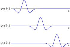
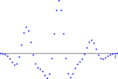
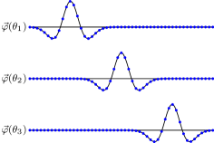
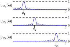
• Deconvolution of point sources: Deconvolution consists of estimating a signal from samples of its convolution with a fixed kernel $K$. When the signal is modeled as a superposition of point sources or spikes, representing fluorescent probes in microscopy [5, 52], celestial bodies in astronomy [75] or interfaces between geological layers in seismography [82], this is an SNL problem where $\theta_{1}$, …, $\theta_{k}$ are the locations of the spikes. In that case, $\varphi_{t}\left(\theta\right)$ is a shifted copy of the convolution kernel $K\left(t-\theta\right)$, as illustrated in the top row of Figure 1.

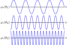
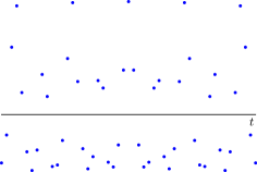
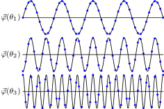
• Spectral super-resolution: Super-resolving the spectrum of a multisinusoidal signal from samples taken over a short period of time is an important problem in communications, radar, and signal processing [85]. This is an SNL problem where $\varphi_{t}\left(\theta\right)$ is a complex exponential $\exp\left(-i2\pi\theta t\right)$ with frequency $\theta$ (see the second row of Figure 1).

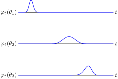
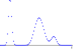
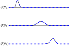
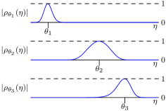
• Heat-source localization: Finding the position of several heat sources in a material with known conductivity from temperature measurements is an SNL problem where $\varphi_{t}\left(\theta\right)$ is the Green’s function of the heat equation parametrized by the location $\theta$ of a particular heat source [57]. The bottom row of Figure 1 shows an example (see Section 4.1 for more details).

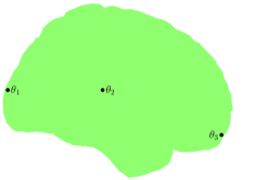
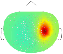
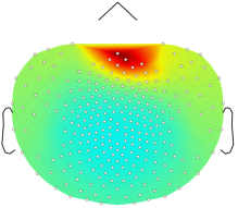
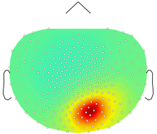
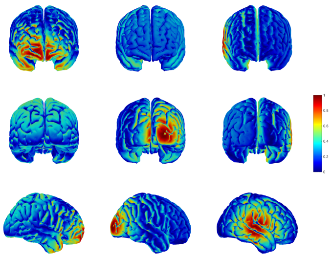
• Estimation of neural activity: Electroencephalography measurements of the electric potential field on the surface of the head can be used to detect regions of focalized activity in the brain [68]. The data are well approximated by an SNL model where the parameters are the locations of these regions [64]. The function $\varphi_{t}\left(\theta\right)$ represents the potential at a specific location $t$ on the scalp, which originates from neural activity at position $\theta$ in the brain. This function can be computed by solving the Poisson differential equation taking into account the geometry and electric properties of the head [70]. Figure 2 shows an example. See Section 4.2 for more details.

• Quantitative magnetic-resonance imaging: The magnetic-resonance relaxation times $T_{1}$ and $T_{2}$ of biological tissues govern the local fluctuations of the magnetic field measured by MR imaging systems [69]. MR fingerprinting is a technique to estimate these parameters by fitting an SNL model where each component corresponds to a different tissue [60, 63, 90]. In this case, the parameter $\theta\in\mathbb{R}^{2}$ encodes the values of $T_{1}$ and $T_{2}$ and the function $\varphi_{t}\left(\theta\right)$ can be computed by solving the Bloch differential equations [7].

1.2 Reformulation as a Sparse-Recovery Problem

A natural approach to estimate the parameters of an SNL model is to solve the nonlinear least-squares problem,

$$\underset{\tilde{\theta}_{1},\ldots,\tilde{\theta}_{k}\in\mathbb{R}^{p},\;\tilde{c}\in\mathbb{R}^{k}}{\operatorname{minimize}}\quad\left\|y-\sum_{i=1}^{k}\tilde{c}_{i}\vec{\varphi}(\tilde{\theta}_{i})\right\|_{2}^{2}.$$ (1.3)

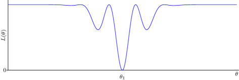
Unfortunately, the resulting cost function is typically nonconvex and has local minima, as illustrated by the simple example in Figure 3. Consequently, local-descent methods do not necessarily recover the true parameters, even in the absence of noise, and global optimization becomes intractable unless $k$ is very small.

Alternatively, we can reformulate the SNL problem as a sparse-recovery problem and leverage $\ell_{1}$-norm minimization to solve it. This approach was pioneered in the 1970s by geophysicists working on spike deconvolution in the context of reflection seismology [92, 23, 55, 80, 25]. Since then, it has been applied to many SNL problems such as acoustic sensing [100, 4], radar [74, 91], electroencephalography (EEG) [83, 98], positron emission tomography (PET) [49, 76, 51], direction of arrival [61, 8], quantitative magnetic resonance imaging  [63, 90], and source localization [57, 62, 72]. Our goal is to provide a theory of sparse recovery via convex optimization explaining the empirical success of this approach.

Figure 3: Nonlinear least-squares cost functions associated to deterministic SNL problems often have non-optimal local minima. The graph depicts the landscape of the nonlinear least squares cost function $L(\theta)=\min_{\tilde{c}\in\mathbb{R}}\left\|\vec{\varphi}(\theta_{1})-\tilde{c}\vec{\varphi}(\theta)\right\|_{2}^{2}$ associated to a deconvolution problem, where the data is generated by convolving a Ricker wavelet [78] with a single spike located $\theta_{1}$. In addition to the global minimum at $\theta_{1}$ there are several spurious local minima.

Let us represent the parameters $\theta_{1}$, …, $\theta_{k}\in\mathbb{R}^{p}$ of an SNL model as a superposition of Dirac measures or spikes in $\mathbb{R}^{p}$, interpreted as a $p$-dimensional parameter space, (1.2),

$$\mu:=\sum_{i=1}^{k}c_{i}\delta_{\theta_{i}},$$ (1.4)

where $\delta_{\theta_{i}}$ denotes a Dirac measure supported at $\theta_{i}$. Intuitively, the atomic measure $\mu$ is a signal that encodes the parameters of interest and their corresponding coefficients. The data described by Equation 1.2 can now be expressed as

$$y=\int_{\mathbb{R}^{p}}\vec{\varphi}(\theta)\mu(\text{d}\theta).$$ (1.5)

The SNL problem is equivalent to recovering $\mu$ from these linear measurements. The price we pay for linearizing is that the linear inverse problem is extremely underdetermined: $y$ has dimension $n$, but $\mu$ lives in a continuous space of infinite dimensionality! To solve the problem, we need to exploit the assumption that the data only depends on a small number of parameters or, equivalently, that $\mu$ is sparse.

For an SNL problem to be well posed, $\theta_{1}$, …, $\theta_{k}$ should be the only set of $k$ or less parameters such that Equation 1.2 holds. In that case, $\mu$ is the solution to the sparse-recovery problem

$$\underset{\tilde{\mu}}{\operatorname{minimize}} \left|\operatorname{support}\left(\tilde{\mu}\right)\right|$$ (1.6)

subject to $$\int_{\mathbb{R}^{p}}\vec{\varphi}(\theta)\tilde{\mu}(\text{d}\theta)=y,$$

where minimization occurs over the set of measures in $\mathbb{R}^{p}$. The cardinality of the support of an atomic measure is a nonconvex function, which is notoriously challenging to minimize. A fundamental insight underlying many approaches to sparse estimation in high-dimensional statistics and signal processing is that one can bypass this difficulty by replacing the nonconvex function with a convex counterpart. In particular, minimizing the $\ell_{1}$ norm instead of the cardinality function has proven to be very effective in many applications.

In order to analyze the application of $\ell_{1}$-norm minimization to SNL problems, we consider a continuous setting, where the optimization variable is a measure supported on a continuous domain. The goal is to obtain an analysis that is valid for arbitrarily fine discretizations of the domain. This is important because, as we will see below, a fine discretization results in a highly-correlated linear operator, which violates the usual assumptions made in the literature on sparse recovery.

In the case of measures supported on a continuous domain, the continuous counterpart of the $\ell_{1}$ norm is the total-variation (TV) norm [79, 40]. Indeed, the TV norm of the atomic measure $\mu$ in Equation 1.4 equals the $\ell_{1}$ norm of its coefficients $\left\|c\right\|_{1}$. Just as the $\ell_{1}$ norm is the dual norm of the $\ell_{\infty}$ norm, the TV norm is defined by

$$\left\|\mu\right\|_{\operatorname{TV}}:=\sup_{f\in\mathcal{C},~{}\left\|f\right\|_{\infty}\leq 1}\left|\int f\,\text{d}\mu\right|,$$ (1.7)

where the supremum is taken over all continuous functions in the unit $\mathcal{L}_{\infty}$-norm ball. Replacing the cardinality function by this sparsity-promoting norm yields the following convex program

$$\underset{\tilde{\mu}}{\operatorname{minimize}} \left\|\tilde{\mu}\right\|_{\operatorname{TV}}$$ (1.8)

subject to $$\int_{\mathbb{R}^{p}}\vec{\varphi}(\theta)\tilde{\mu}(\text{d}\theta)=y.$$

The goal of this paper is to understand when the solution to Problem (1.8) exactly recovers the parameters of an SNL model.

1.3 Compressed Sensing

Section 1.2 shows that solving an SNL problem is equivalent to recovering a sparse signal from linear underdetermined measurements. This is reminiscent of compressed sensing [27, 20, 42]. In its most basic formulation, the goal of compressed sensing is to estimate a signal $x\in\mathbb{R}^{m}$ with $k$ nonzeros from linear measurements $y\in\mathbb{R}^{n}$ given by $y:=Ax$, where $A\in\mathbb{R}^{n\times m}$ and $m>n$. Remarkably, exact recovery of $x$ is still possible under certain conditions on the matrix $A$, even though the linear system is underdetermined.

Overdetermined linear inverse problems are said to be ill posed when the measurement matrix is ill conditioned. This occurs when there exist vectors that lie close to the null space of the matrix, or equivalently when a subset of its columns is highly correlated. Analogously, the compressed-sensing problem is ill posed if any sparse subset of columns is highly correlated, because this implies that sparse vectors lie close to the null space. Early works on compressed sensing derive recovery guarantees assuming a bound on the maximum correlation between the columns of the measurement matrix $A$ (sometimes called incoherence). They prove that tractable algorithms such as $\ell_{1}$-norm minimization and greedy techniques achieve exact recovery as long as the maximum correlation is of order $n^{-1/2}$ for sparsity levels $k$ of up to order $\sqrt{n}$ [28, 31, 48, 93], even if the data are corrupted by additive noise [30, 94]. These results were subsequently strengthened to sparsity levels of order $n$ (up to logarithmic factors) [27, 67, 18, 6, 12] under stricter assumptions on the conditioning of sparse subsets of columns in the measurement matrix, such as the restricted-isometry property [18] or the restricted-eigenvalue condition [6].

Figure 4: Columns and intercolumn correlations for a typical compressed-sensing matrix $A\in\mathbb{R}^{100\times 300}$ with i.i.d. standard Gaussian entries. The notation $A_{i}$ denotes the $i$th column of $A$. Note that $|A_{i}^{T}A_{j}|$ is small whenever $i\neq j$.

The question is whether compressed-sensing theory applies to SNL problems. Let us consider an SNL problem where the parameter space is discretized to yield a finite-dimensional version of the sparse-recovery problem described in Section 1.2. The measurement model in Equation 1.5 can then be expressed as

$$y =\sum_{j=1}^{m}\vec{\varphi}(\eta_{j})x_{j}$$ (1.9)

$$=\Phi x.$$ (1.10)

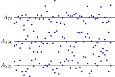
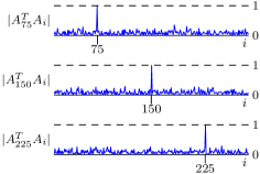
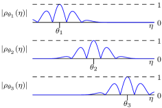
$\Phi$ is a measurement matrix whose columns correspond to the feature vectors of $\eta_{1}$, …, $\eta_{m}\in\mathbb{R}^{p}$, which denote the $m$ points of the discretized parameter space. The signal $x\in\mathbb{R}^{m}$ is the discrete version of $\mu$ in Equation 1.4: a sparse vector, such that $x_{i}=c_{j}$ when $\eta_{j}=\theta_{i}$ for some $i\in\left\{1,\ldots,k\right\}$ and $x_{j}=0$ otherwise. For compressed-sensing theory to apply here, the intercolumn correlations of $\Phi$ should be very low. Figure 4 shows the intercolumn correlations of a typical compressed-sensing matrix: each column is almost uncorrelated with every other column. Figures 5 and 6 show the correlation function $\rho_{\theta}:\mathbb{R}^{p}\rightarrow\mathbb{R}$

$$\rho_{\theta}(\eta):=\left\langle\vec{\varphi}(\theta),\vec{\varphi}(\eta)\right\rangle,$$ (1.11)

for the different SNL problems discussed in Section 1.1. The intercolumn correlations of the measurement matrix $\Phi$ in the corresponding discretized SNL problems are given by samples of $\rho_{\eta_{i}}$ at the locations of the remaining grid points $\eta_{j}$, $i\neq j$. The contrast with the intercolumn structure of the compressed-sensing matrix is striking: nearby columns in all SNL measurement matrices are very highly correlated. This occurs under any reasonable discretization of the parameter space; discretizing very coarsely would result in inaccurate parameter estimates, defeating the whole point of solving the SNL problem.

Deconvolution
Super-resolution
Heat-Source Localization

Figure 5: Correlation structure of the measurement operators arising in deconvolution, super-resolution, and heat-source localization. The left column shows the discrete data $\vec{\varphi}(\theta_{i})$ for three parameter values. The right column gives the absolute values of the corresponding correlation functions $\rho_{\theta_{i}}(\eta)=\vec{\varphi}(\theta_{i})^{T}\vec{\varphi}(\eta)$.

$\rho_{\theta_{1}}$                                           $\rho_{\theta_{2}}$                                           $\rho_{\theta_{3}}$

Figure 6: Example of correlation functions for the electroencephalography brain-activity localization problem. Each column shows three views of the correlation function $\rho_{\theta_{i}}(\eta)=\vec{\varphi}(\theta_{i})^{T}\vec{\varphi}(\eta)$, $i=1,2,3$, corresponding to one of the neural-activity sources shown in Figure 2.

The difference between the correlation structure of the measurement matrix in compressed-sensing and SNL problems is not surprising. The entries of compressed-sensing matrices are random. As a result, small subsets of columns are almost uncorrelated with high probability. In contrast, matrices in discretized SNL problems arise from a deterministic model tied to an underlying continuous parameter space and to a function $\varphi_{t}$ that is typically smooth. Since $\varphi_{t}\left(\theta\right)\approx\varphi_{t}\left(\theta^{\prime}\right)$ when $\theta\approx\theta^{\prime}$, nearby columns are highly correlated. These matrices do not satisfy any of the properties of the conditioning of sparse submatrices commonly assumed in compressed sensing. In conclusion, the answer to our previous question is a resounding no: compressed-sensing theory does not apply to SNL problems.

1.4 Beyond Sparsity and Randomness: Separation and Correlation Decay

The fact that compressed-sensing theory does not apply to SNL problems involving deterministic measurements is not a theoretical artifact. Sparsity is not a strong enough condition to ensure that such SNL problems are well posed. If $\varphi_{t}$ is smooth, which is usually the case in applications, the features $\vec{\varphi}\left(\theta\right)$ corresponding to parameters that are clustered in the parameter space are highly correlated. This can be seen in the correlation plots of Figures 5 and 6. As a result, different sparse combinations of features may yield essentially the same data. For a detailed analysis of this issue in the context of super-resolution and deconvolution of point sources we refer the reader to Section 3.2 in [14] (see also [65] and [84]) and Section 2.1 in [3], respectively.

Additional assumptions beyond sparsity are necessary to establish recovery guarantees for SNL problems. At the very least, the features $\vec{\varphi}\left(\theta_{1}\right)$, …, $\vec{\varphi}\left(\theta_{k}\right)$ in the data cannot be too correlated. For arbitrary SNL problems it is challenging to define simple conditions to preclude this from happening. However, in most practical situations, SNL problems exhibit correlation decay, meaning that the correlation function $\rho_{\theta}$ defined in Equation 1.11 is bounded by a decaying function away from $\theta$. This is a natural property: the more separated two parameters $\theta$ and $\theta^{\prime}$ are in the parameter space, the less correlated we expect their features $\vec{\varphi}\left(\theta\right)$ and $\vec{\varphi}\left(\theta^{\prime}\right)$ to be. All the examples in Section 1.1 have correlation decay (see Figures 5 and 6).

For SNL problems with correlation decay there is a simple way of ensuring that the features corresponding to the true parameters $\theta_{1}$, …, $\theta_{k}$ are not highly correlated: imposing a minimum separation between them in the parameter space. The main contribution of this paper is showing that this is in fact sufficient to guarantee that TV-norm minimization achieves exact recovery, under some additional conditions on the derivatives of the correlation function.

1.5 Organization

In Section 2 we propose a theoretical framework for the analysis of sparse estimation in the context of SNL inverse problems. We focus on the case $p=1$ for simplicity, but our results can be extended to higher dimensions, as described in Section 3.5. Our main results are Theorems 2.4 and 2.6, which establish exact-recovery results for SNL problems with correlation decay under a minimum separation on the true parameters. Section 3 contains the proof of these results, which are based on a novel dual-certificate construction. Section 4 illustrates the theoretical results through numerical experiments for two applications: heat-source localization and estimation of brain activity from electroencephalography data.

2 Main Results

2.1 Correlation decay

In this section we formalize the notion of correlation decay by defining several conditions on the correlation function $\rho_{\theta}$ and on its derivatives. Throughout we assume that the problem is one dimensional ($p:=1$).

To alleviate notation we define

$$\rho_{\theta}^{(q,r)}(\eta):=\vec{\varphi}^{\,(q)}(\theta)^{T}\vec{\varphi}^{\,(r)}(\eta),$$ (2.1)

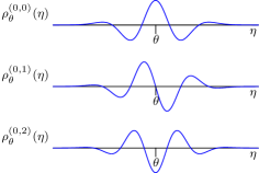
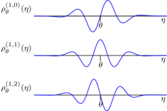
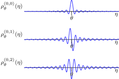
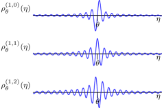
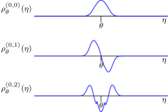
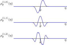
for $q=0,1$ and $r=0,1,2$, where $\vec{\varphi}^{\,(q)}$ is the $q$th derivative of $\vec{\varphi}$. Recall that we assume $\|\vec{\varphi}(\theta)\|_{2}=1$ for all $\theta\in\mathbb{R}$. This implies $\rho_{\theta}(\theta)=1$ and $\rho^{(1,0)}_{\theta}(\theta)=\rho^{(0,1)}_{\theta}(\theta)=0$ for all $\theta\in\mathbb{R}$. Plots of these derivatives are shown in Figure 8 for the deconvolution, super-resolution, and heat-source localization problems. Our conditions take the form of bounds in different regions of the parameter space: a near region, an intermediate region, and a far region, as depicted in Figure 7.

Figure 7: Illustration of the near, intermediate and decay conditions on the correlation function defined in Section 2.1. This example shows a correlation function arising in deconvolution.

In the near region the correlation can be arbitrarily close to one, but is locally bounded by a quadratic function.

Condition 2.1 (Near Condition).

The correlation function $\rho_{\theta}$ satisfies the near condition if

$$\rho_{\theta}^{(0,2)}(\eta) \leq-\gamma_{0}\quad\text{and}$$ (2.2)

$$|\rho_{\theta}^{(1,2)}(\eta)| \leq\gamma_{1}\left\|\vec{\varphi}^{\,(1)}(\theta)\right\|_{2}^{2}$$ (2.3)

hold for all $\eta$ in $[N^{-},N^{+}]$, where $N^{\pm}:=\theta\pm N$, and $\gamma_{0},\gamma_{1}$ are positive constants.

Equation (2.2) requires correlations to be concave locally, which is natural since the maximum of $\rho_{\theta}$ is attained at $\theta$. Equation (2.3) is a regularity condition that requires $\rho_{\theta}^{(0,2)}(\eta)$ to vary smoothly as we change the center $\theta$. The normalization quantity $\left\|\vec{\varphi}^{\,(1)}(\theta)\right\|_{2}^{2}$ captures how sensitive the features $\vec{\varphi}$ are to perturbations. If this quantity is small for some $i$ then we require more regularity from $\rho_{\theta}$ because $\theta$ is harder to distinguish from nearby points using the measurements $\vec{\varphi}$.

In the intermediate region the correlation function $\rho_{\theta}$ is bounded but can otherwise fluctuate arbitrarily. In addition, we require a similar constraint on its derivative with respect to the position of the center $\theta$.

Condition 2.2 (Intermediate Condition).

The correlation function $\rho_{\theta}$ satisfies the intermediate condition if

$$|\rho_{\theta}^{(0,0)}(\eta)| \leq\gamma_{2}<1\quad\text{and}$$ (2.4)

$$|\rho_{\theta}^{(1,0)}(\eta)| \leq\gamma_{3}\left\|\vec{\varphi}^{\,(1)}(\theta)\right\|_{2}^{2}$$ (2.5)

hold for $\eta<N^{-}$ and $\eta>N^{+}$, where $N^{\pm}$ are defined as in the near condition, and $\gamma_{2},\gamma_{3}$ are positive constants.

Deconvolution
Super-resolution
Heat-Source Localization

Figure 8: Derivatives of the correlation functions arising in deconvolution, super-resolution, and heat-source localization. In all cases the correlation function is locally concave and all derivatives exhibit decaying tails. In the case of super-resolution the tail decay is not summable, but can be made summable by applying a window function to the measurements.

In the decay region the correlation and its derivatives are bounded by a decaying function.

Condition 2.3 (Decay Condition).

The correlation function $\rho_{\theta}$ satisfies the decay condition with decay constant $\sigma>0$ if

$$|\rho_{\theta}^{(0,r)}(\eta)| \leq C_{0,r}e^{-(|\eta-\theta|-D)/\sigma}\quad\text{and}$$ (2.6)

$$|\rho_{\theta}^{(1,r)}(\eta)| \leq C_{1,r}e^{-(|\eta-\theta|-D)/\sigma}\left\|\vec{\varphi}^{\,(1)}(\theta)\right\|_{2}^{2}$$ (2.7)

hold for $\eta<D^{-}$ and $\eta>D^{+}$, where $r=0,1,2$, $D^{\pm}:=\theta\pm D$, and $C_{q,r}$ are positive constants.

The choice of exponential decay is for concreteness, and can be replaced by a different summable decay bound. Figure 8 shows the derivatives of the correlation functions for several SNL problems.

Dense Uniform	Irregular
Sparse Uniform	Right Side Only

Figure 9: Plots of the correlation function $\rho_{\theta}(\eta)$ for a deconvolution problem with varying sampling patterns (indicated by the x markers on the horizontal axis). Specifically, $\vec{\varphi}(\theta)_{i}:=\exp(-(\theta-s_{i})^{2}/2)$ are samples from a $\theta$-centered Gaussian kernel. In the dense uniform case, the correlation function satisfies Conditions 2.1, 2.2 and 2.3. For irregular sampling pattern, the correlation function will in general satisfy the conditions if there are some samples close to $\theta$. For sparse uniform samples, the correlation function is nearly flat at $\theta$ since there are too few measurements to distinguish nearby parameters. If the samples are only located to the right of $\theta$, then all parameters on the left side have nearly identical measurements.

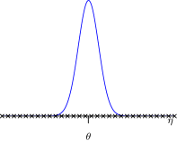
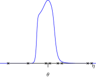
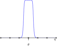
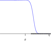
The sample locations $s_{1},\ldots,s_{n}$ have a direct effect on the correlation function, and hence on whether an SNL problem satisfies Conditions 2.1, 2.2 and 2.3. In Figure 9 we depict the correlation function $\rho_{\theta}$ for different sampling patterns in a Gaussian deconvolution problem with $\vec{\varphi}(\theta)_{i}:=\exp(-(\theta-s_{i})^{2}/2)$. For both regular and irregular sampling patterns, the correlation functions are well behaved as long as there are samples close to the true parameter. In contrast, when there are few samples, or the samples are distant from the true parameter, the conditions in Conditions 2.1, 2.2 and 2.3 may be violated. We refer the interested reader to [3] for a more precise analysis of sampling patterns for deconvolution of point sources.

2.2 Exact Recovery for SNL Problems with Uniform Correlation Decay

In this section we focus on SNL problems where the correlation function $\rho_{\theta}$ of the measurement operator is approximately translation invariant, meaning that $\rho_{\theta}$ has similar properties for any value of $\theta$. Examples of such SNL problems include super-resolution, deconvolution, and heat-source localization if the conductivity is approximately uniform. We prove that TV-norm minimization recovers a superposition of Dirac measures exactly as long as the support satisfies a separation condition related to the decay properties of the correlation function and its derivatives.

Figure 10: Illustration of the minimum-separation condition required by Theorem 2.4.

Theorem 2.4.

Let $\Theta:=\{\theta_{1},\ldots,\theta_{k}\}$ be the support of the measure $\mu$ defined in Equation 1.4. Assume that the correlation functions $\rho_{\theta_{i}}$, $\theta_{i}\in\Theta$, satisfy Conditions 2.1, 2.2 and 2.3 for fixed constants $N$, $D$, $\sigma$, $\gamma\in\mathbb{R}^{4}$, and $C\in\mathbb{R}^{2\times 3}$. Then $\mu$ is the unique solution to Problem (1.8) as long as the minimum separation of $\Theta$ satisfies,

$$\min_{i\neq j,\;\theta_{i},\theta_{j}\in\Theta}\left|\theta_{i}-\theta_{j}\right|>2D+\Delta\sigma,\quad\Delta:=\max\left(\log(1+2(C_{0,0}+C_{1,1})),\lambda_{1},\lambda_{2}\right),$$ (2.8)

where

$$\lambda_{1}=2\log\left(\frac{2(2(2C_{0,0}+C_{1,1}-C_{1,1}\gamma_{2}+C_{0,1}\gamma_{3})+1-\gamma_{2})}{-C_{0,0}+\sqrt{C_{0,0}^{2}+4(1-\gamma_{2})(2(2C_{0,0}+C_{1,1}-C_{1,1}\gamma_{2}+C_{0,1}\gamma_{3})+1-\gamma_{2})}}\right),$$ (2.9)

$$\lambda_{2}=2\log\left(\frac{2(2((2C_{0,0}+C_{1,1})\gamma_{0}+C_{0,2}+C_{0,1}\gamma_{1})+\gamma_{0})}{-C_{0,2}+\sqrt{C_{0,2}^{2}+4\gamma_{0}(2((2C_{0,0}+C_{1,1})\gamma_{0}+C_{0,2}+C_{0,1}\gamma_{1})+\gamma_{0})}}\right),$$ (2.10)

and the constants $C_{q,r}$ are chosen so that

$$C_{0,1}C_{1,0} =C_{0,0}C_{1,1},\quad\text{and}$$ (2.11)

$$C_{0,1}C_{1,2} =C_{1,1}C_{0,2}.$$

Note that the condition in Equation 2.11 is only needed to simplify the statement and proof of our results.

Theorem 2.4 establishes that TV minimization recovers the true parameters of an SNL problem when the support separation is larger than a constant that is proportional to the rate of decay of the correlation function and its derivatives. This separation is measured from the edges of the intermediate regions, as depicted in Figure 10. In stark contrast to compressed-sensing theory, the result holds for correlation functions that are arbitrarily close to one in the near regions, and may have arbitrary bounded fluctuations in the intermediate regions.

Our statement and proof of Theorem 2.4 focuses on clarity over sharpness. For example, in the Gaussian deconvolution problem depicted in Figure 9 with dense uniform samples, the theorem requires a minimum separation of approximately $6.6$ to guarantee exact parameter recovery. To obtain this bound, we let $N=1$, $D=0$, $\sigma=1$,

$$\gamma=\begin{bmatrix}0.185&0.983&0.788&0.868\end{bmatrix}^{T},\quad C=\begin{bmatrix}2.818&3.348&4.200\\ 6.786&8.060&10.113\end{bmatrix},$$ (2.12)

and verify the conditions numerically. This is in contrast with the minimum separation of approximately $3$ proven in [3]. Part of this discrepancy comes from applying exponential decay bounds to a Gaussian-shaped correlation function.

Our result requires conditions on the correlation functions centered at the true support $\Theta$, and also on their derivatives. The decay conditions on the derivatives constrain the correlation structure of the measurement operator when we perturb the position of the true parameters. For example, they implicitly bound pairwise correlations centered in a small neighborhood of the support. Exploring to what extent these conditions are necessary is an interesting question for future research.

Figure 11: Support-centered correlations with varying decay parameters for the heat-source localization problem. The vertical dashed lines indicate the locations of $D_{i}^{\pm}$ for $i=1,2,3$, whereas the curved dashed lines indicate the exponential decay bounds. As we move from left to right along the $\theta$-axis the thermal conductivity is decreasing, which causes the correlation functions to become narrower.

2.3 Exact Recovery for SNL Problems with Nonuniform Correlation Decay

The measurement operators associated to many SNL problems of practical interest have nonuniform correlations. Figures 5 and 6 show that this is the case for heat-source localization with spatially-varying conductivity, and for estimation of brain-activity from EEG data. Our goal in this section is to establish recovery guarantees for such problems.

The conditions on the correlation structure of the measurement operator required by Theorem 2.4 only pertain to the correlation functions centered at the true parameters. In order to generalize the result, we allow the correlation function centered at each parameter to satisfy the conditions in Section 2.1 with different constants. This makes it possible for the correlation to have near and intermediate regions of varying widths around each element of the support, as well as different decay constants in the far region. Our main result is that TV-norm minimization achieves exact recovery for SNL problems with nonuniform correlation structure, as long as the support satisfies a minimum-separation condition dependent on the corresponding support-centered correlation functions.

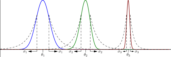
Let $\Theta$ be the support of our signal of interest, and assume $\rho_{\theta_{i}}$ satisfies the decay conditions in Section 2.1 with parameters $\sigma_{i}$, $D_{i}$, and $N_{i}$, which are different for all $\theta_{i}\in\Theta$. Extending the notation, we let $N_{i}^{\pm}:=\theta_{i}\pm N_{i}$ and $D_{i}^{\pm}:=\theta_{i}\pm D_{i}$ denote the endpoints of the near and decay regions, respectively. Intuitively, when $\sigma_{i}$ and $D_{i}$ are small, the corresponding correlation function $\rho_{\theta_{i}}$ is “narrower” and should require less separation than “wider” correlation functions with large values of $\sigma_{i}$ and $D_{i}$. This is illustrated in Figure 11, where we depict $\rho_{\theta_{i}}$ for the heat-source localization problem at three different values of $i$. The decay becomes more pronounced towards the right due to the changing thermal conductivity of the underlying medium. For the problem to be well posed, one would expect $\theta_{1}$ to require more separation from other active sources than $\theta_{2}$, which in turn should require more than $\theta_{3}$. We confirm this intuition through numerical experiments in Section 4.1. To make it mathematically precise, we define the following generalized notion of support separation.

Definition 2.5 (Generalized support Separation).

Suppose for all $\theta_{i}\in\Theta$ that $\rho_{\theta_{i}}$ satisfies Condition 2.3 with parameters $D_{i}$ and $\sigma_{i}$. Define the normalized distance $d(\theta_{i},\theta_{j})$ for $i\neq j$ by

$$d(\theta_{i},\theta_{j})=\frac{|\theta_{i}-\theta_{j}|-D_{i}-D_{j}}{\max(\sigma_{i},\sigma_{j})}.$$ (2.13)

Assume that $\Theta$ is ordered so that $\theta_{1}<\theta_{2}<\cdots<\theta_{{k}}$. $\Theta$ has separation $\Delta>0$ if $d(\theta_{i},\theta_{j})>|i-j|\Delta$ for all $\theta_{i},\theta_{j}\in\Theta$ with $i\neq j$.

The normalized distance $d(\theta_{i},\theta_{j})$ is measured between the edges of the decay regions of $\theta_{i}$ and $\theta_{j}$, and normalized by the level of decay. This allows sharply decaying correlation functions to be in close proximity with one another. We require $d(\theta_{i},\theta_{j})>|i-j|\Delta$ to prevent the parameters from becoming too clustered. If we only require the weaker condition $d(\theta_{i},\theta_{j})>\Delta$, and if $\sigma_{i}$ grows very quickly with $i$, then we could have $d(\theta_{1},\theta_{j})\approx\Delta$ for all $j>i$. This causes too much overlap between the correlation functions.

Figure 12: Illustration of the generalized support-separation condition in Definition 2.5.

Figure 13: Non-trivial configuration allowed by Definition 2.5. The central parameter $\theta_{4}$ has weaker decay, and thus requires more separation from the other parameters.

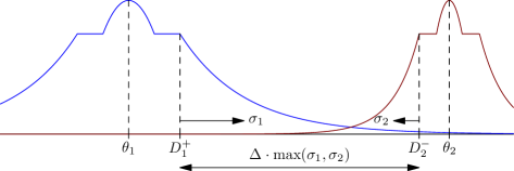
Figure 13 gives an example of parameters and correlation functions that satisfy the conditions of Definition 2.5. The following theorem establishes exact-recovery guarantees under a condition on the generalized support separation.

Theorem 2.6.

Suppose that for all $\theta_{i}\in\Theta$ that $\rho_{\theta_{i}}$ satisfies Conditions 2.1, 2.2 and 2.3 and (2.11) with constants $N:=N_{i}$, $D:=D_{i}$, $\sigma:=\sigma_{i}$, $C$, and $\gamma$. Note that $C$ and $\gamma$ are the same for each $\theta_{i}$. Then the true measure $\mu$ defined in (1.4) is the unique solution to Problem (1.8) when $\Theta$ has separation $\Delta$ (as determined by Definition 2.5) satisfying

$$\Delta>\max\left(\log(1+2(C_{0,0}+C_{1,1})),\lambda_{1},\lambda_{2}\right),$$ (2.14)

(2.9), (2.10), and (2.11).

The proof of Theorem 2.6, which implies Theorem 2.4, is given in Section 3. The theorem establishes that TV minimization recovers the true parameters of SNL problems with nonuniform correlation decays when the generalized support separation is larger than a constant. Equivalently, exact recovery is achieved as long as each true parameter $\theta_{i}$ is separated from the rest by a distance that is proportional to the rate of decay of the correlation function centered at $\theta_{i}$. The separation is measured from the edges of the intermediate regions, which can also vary in width as depicted in Figure 10. The result matches our intuition about SNL problems: the parameters can be recovered as long as they yield measurements that are not highly correlated. As mentioned previously, the theorem requires decay conditions on the derivatives of the correlation function, which constrain the correlation structure of the measurement operator.

2.4 Robustness to Noise

In practice, measurements are always corrupted by noisy perturbations. Noise can be taken into account in our measurement model (1.2) by incorporating an additive noise vector $z\in\mathbb{R}^{n}$:

$$y:=\sum_{i=1}^{k}c_{i}\vec{\varphi}(\theta_{i})+z.$$ (2.15)

To adapt the TV-norm minimization problem (1.8) to such measurements, we relax the data consistency constraint from an equality to an inequality:

$$\underset{\tilde{\mu}}{\operatorname{minimize}} \left\|\tilde{\mu}\right\|_{\operatorname{TV}}$$ (2.16)

subject to $$\left\|\int_{\mathbb{R}^{p}}\vec{\varphi}(\theta)\tilde{\mu}(\text{d}\theta)-y\right\|_{2}\leq\xi,$$

where $\xi>0$ is a parameter that must be tuned according to the noise level. Previous works have established robustness guarantees for TV-norm minimization applied to specific SNL problems such as super-resolution [37, 15] and deconvolution [3] at small noise levels. These proofs are based on dual certificates. Combining the arguments in [37, 3] with our dual-certificate construction in Section 3 yields robustness guarantees for general SNL problems in terms of support recovery at high signal-to-noise regimes. We omit the details, since the proof would essentially mimic the ones in [37, 3]. In Figure 14 we show an application of Equation 2.16 to a noisy deconvolution problem taken from [3].

Figure 14: Deconvolution from noisy samples (in red) with a signal-to-noise ratio of 20.7 dB for the Ricker wavelet. The noise is iid Gaussian. The recovered signals are obtained by solving equation 2.16 on a fine grid which contains the location of the original spikes.

2.5 Discretization

The continuous optimization problem (2.16) can be solved by applying $\ell_{1}$-norm minimization after discretizing the parameter space. This is a very popular approach in practice for a variety of SNL problems [61, 92, 100, 83, 90]. If the true parameters lie on the discretization grid, then our exact-recovery results translate immediately. The following corollary is a discrete version of Theorem 2.6.

Corollary 2.7.

Assume $\Theta$ lies on a known discretized grid $G:=\{\eta_{1},\ldots,\eta_{m}\}$ so that $\Theta\subset G$. Furthermore, suppose the conditions of Theorem 2.6 hold so that $\mu$ as defined in (1.4) is the unique solution to Problem (1.8). Define the dictionary $\Phi\in\mathbb{R}^{n\times m}$ by

$$\Phi:=\begin{bmatrix}\vec{\varphi}(\eta_{1})&\cdots&\vec{\varphi}(\eta_{m})\end{bmatrix}.$$ (2.17)

Then the $\ell_{1}$-norm minimization problem

$$\underset{\tilde{x}}{\operatorname{minimize}} \left\|\tilde{x}\right\|_{1}$$ (2.18)

$$\operatorname{subject~{}to} \Phi\tilde{x}=y$$

has a unique solution $x\in\mathbb{R}^{m}$ satisfying

$$x_{j}:=\begin{cases}c_{i}&\text{if $\eta_{j}=\theta_{i}$,}\\ 0&\text{otherwise,}\end{cases}$$ (2.19)

for $j=1,\ldots,m$.

Proof.

If the support of $\tilde{\mu}$ in Problem (1.8) is restricted to lie on $G$, then Problems (1.8) and (2.18) are the same. Thus $\left\|\mu\right\|_{\operatorname{TV}}$ must be smaller than $\left\|\tilde{x}\right\|_{1}$ for any $\tilde{x}$ such that $\Phi\tilde{x}=y$. By assumption $\mu$ is supported on $G$, so the result follows. ∎

Of course, the true parameters may not lie on the grid used to solve the $\ell_{1}$-norm minimization problem. The proof techniques used to derive robustness guarantees for super-resolution and deconvolution in [37, 3] can be leveraged to provide some control over the discretization error. Performing a more accurate analysis of discretization error for SNL problems is an interesting direction for future research.

2.6 Related Work

2.6.1 Sparse Recovery via Convex Programming from Deterministic Measurements

In [29], Donoho and Elad develop a theory of sparse recovery from generic measurements based on the spark and coherence of the measurement matrix $\Phi$. The spark is defined to be the smallest positive value $s$ such that $\Phi$ has $s$ linearly dependent columns. The coherence, which we denote by $M(\Phi)$, is the maximum absolute correlation between any two columns of $\Phi$. The authors show that exact recovery is achieved by $\ell_{1}$-minimization when the number of true parameters is less than $(1+1/M(\Phi))/2$. As discussed in Section 1.3, these arguments are inapplicable to the finely-discretized parameter spaces occurring in SNL problems since neighboring columns of $\Phi$ have correlations approaching one. In [32], the authors provide a support-dependent condition for exact recovery of discrete vectors. Using our notation, they require that $\beta(\Theta)/(1-\alpha(\Theta))<1$ where

$$\alpha(\Theta):=\max_{\theta_{i}\in\Theta}\sum_{\theta_{k}\in\Theta,k\neq i}|\vec{\varphi}(\theta_{i})^{T}\vec{\varphi}(\theta_{k})|\quad\text{and}\quad\beta(\Theta):=\max_{\eta_{j}\notin\Theta}\sum_{\theta_{k}\in\Theta}|\vec{\varphi}(\eta_{j})^{T}\vec{\varphi}(\theta_{j})|.$$ (2.20)

Here $\vec{\varphi}(\eta_{j})$ for $\eta_{j}\notin\Theta$ ranges over the columns of $\Phi$ that do not correspond to the true parameters. This condition is also inapplicable for matrices arising in our problems of interest because $\beta(\Theta)$ approaches one (or larger) for finely-discretized parameter spaces. Sharper exact-recovery guarantees in subsequent works [22, 27, 67, 18, 6, 12] require randomized measurements, and therefore do not hold for deterministic SNL problems as explained in Section 1.3.

2.6.2 Convex Programming Applied to Specific SNL Problems

In [14, 38], the authors establish exact recovery guarantees for super-resolution via convex optimization by leveraging parameter separation (see Section 1.4). Subsequent works build upon these results to study the robustness of this methodology to noise [89, 37, 15, 34], missing data [87], and outliers [39]. A similar analysis is carried out in [3] for deconvolution. The authors establish a sampling theorem for Gaussian and Ricker-wavelet convolution kernels, which characterizes what sampling patterns yield exact recovery under a minimum-separation condition. Other works have analyzed the Gaussian deconvolution problem under nonnegativity constraints [81, 35], and also for randomized measurements [73]. All of these works exploit the properties of specific measurement operators. In contrast, the present paper establishes a general theory that only relies on the correlation structure of the measurements. The works that are closer to this spirit are [2, 88], which analyze deconvolution via convex programming for generic convolution kernels. The results in [2] require quadratically decaying bounds on the first three derivatives of the convolution kernel. In [88], the authors prove exact recovery assuming bounds on the first four derivatives of the autocorrelation function of the convolution kernel. In contrast to these works, our results allow for discrete irregular sampling and for measurement operators that are not convolutional, which is necessary to analyze applications such as heat-source localization or estimation of brain activity.

Algorithms for solving the convex programs arising from SNL problems divide into two categories: grid-based and grid-free (or off-the-grid). In grid-based methods the parameter space is discretized, thus yielding a finite-dimensional $\ell_{1}$ minimization problem that can be solved using standard methods (as we have done in Section 4). Grid-free methods attempt to directly solve the infinite-dimensional, but with weaker guarantees (see [53] and [58] for review articles). Recently, several authors [26, 36, 10] have proposed grid-free algorithms based on the conditional gradient method [43].

2.6.3 Other Methodologies

SNL parameter recovery can be formulated as a nonlinear least squares problem [45]. For a fixed value of the parameters $\theta_{1},\ldots,\theta_{k}$, the optimal coefficients $c_{1},\ldots,c_{k}$ in (1.1) have a closed form solution. This makes it possible to minimize the nonlinear cost function with respect to $\theta_{1},\ldots,\theta_{k}$ directly, a technique known as variable projection [44]. As shown in Figure 3, a downside to this approach is that it may converge to suboptimal local minima, even in the absence of noise.

Prony’s method [24, 85] and the finite-rate-of-innovation (FRI) framework [97, 33] can be applied to tackle SNL problems, as long one can recast them as spectral super-resolution problems. This provides a recovery method that avoids discretizing the parameter space. The FRI framework has also been applied to arbitrary non-bandlimited convolution kernels [95] and nonuniform sampling patterns [71], but without exact-recovery guarantees. These techniques have been recently extended by Dragotti and Murray-Bruce [66] to physics-driven SNL problems. By approximating complex exponentials with weighted sums of Green’s functions, they are able to recast parameter recovery as a related spectral super-resolution problem that approximates the true SNL problem.

3 Proof of Exact-Recovery Results

3.1 Dual Certificates

To prove Theorem 2.6 we construct a certificate that guarantees exact recovery.

Proposition 3.1 (Proof in Appendix A).

Let $\Theta=\{\theta_{1},\ldots,\theta_{k}\}\subset\mathbb{R}$ denote the support of the signed atomic measure $\mu$. Assume that for any sign pattern $\xi\in\{\pm 1\}^{k}$ there is a $\tilde{q}\in\mathbb{R}^{p}$ such that $\widetilde{Q}(\theta):=\tilde{q}^{T}\vec{\varphi}(\theta)$ satisfies

$$\widetilde{Q}(\theta_{i})=\xi_{i}, \quad\quad\forall\theta_{i}\in\Theta,$$ (3.1)

$$|\widetilde{Q}(\theta)|<1, \quad\quad\forall\theta\in\Theta^{c}.$$ (3.2)

Then $\mu$ is the unique solution to problem (1.8).

To prove exact recovery of a signal we need to show that it is possible to interpolate the sign pattern of its amplitudes, which we denote by $\xi$, on its support $\Theta$ using an interpolating function $\widetilde{Q}(\theta)$ that is expressible as a linear combination of the coordinates of $\vec{\varphi}(\theta)$. The coefficient vector of this linear combination, denoted by $\tilde{q}$, is known as a dual certificate in the literature because it certifies recovery and is a solution to the Lagrange dual of problem (1.8):

$$\begin{array}[]{ll}\underset{\nu}{\text{maximize}}&\nu^{T}y\\ \text{subject to}&\sup_{\theta}\left|\nu^{T}\vec{\varphi}(\theta)\right|\leq 1.\end{array}$$ (3.3)

Dual certificates have been widely used to derive guarantees for inverse problems involving random measurements, including compressed sensing [19, 17], matrix completion [11] and phase retrieval [13]. In such cases, the certificates are usually constructed by leveraging concentration bounds and other tools from probability theory [96]. In contrast, our setting is completely deterministic. More recently, dual certificates have been proposed for specific deterministic problems such as super-resolution [14] and deconvolution [3]. Our goal here is to provide a construction that is valid for generic SNL models with correlation decay.

3.2 Correlation-Based Dual Certificates

Our main technical contribution is a certificate that only depends on the correlation function of the measurement operator. In contrast, certificate constructions in previous works on SNL problems [14, 3, 2] typically rely on problem-specific structure, with the exception of [88] which proposes a certificate for time-invariant problems based on autocorrelation functions.

In our SNL problems of interest the function $\vec{\varphi}(\theta)$ mapping the parameters of interest to the data is assumed to be continuous and smooth. As a result, Equations 3.1 and 3.2 imply that any valid interpolating function $\widetilde{Q}$ reaches a local extremum at each $\theta_{i}\in\Theta$. Equivalently, $\widetilde{Q}$ satisfies the following $2k$ interpolation equations for all $\theta_{i}\in\Theta$:

$$\widetilde{Q}(\theta_{i}) =\xi_{i},$$ (3.4)

$$\widetilde{Q}^{(1)}(\theta_{i}) =0.$$ (3.5)

Inspired by this observation, we define

$$q:=\sum_{i=1}^{k}\alpha_{i}\vec{\varphi}(\theta_{i})+\beta_{i}\frac{\vec{\varphi}^{(1)}(\theta_{i})}{\left\|\vec{\varphi}^{(1)}(\theta_{i})\right\|_{2}^{2}}$$ (3.6)

where $\alpha_{i},\beta_{i}\in\mathbb{R}$, $i=1,\ldots,k$, are chosen so that $Q(\theta):=q^{T}\vec{\varphi}(\theta)$ satisfies the interpolation equations. Crucially, this choice of coefficients yields an interpolation function $Q$ that is a linear combination of correlation functions centered at $\Theta$,

$$Q(\theta) =\sum_{i=1}^{k}\alpha_{i}\vec{\varphi}(\theta_{i})^{T}\vec{\varphi}(\theta)+\beta_{i}\frac{\vec{\varphi}^{(1)}(\theta_{i})^{T}\vec{\varphi}(\theta)}{\left\|\vec{\varphi}^{(1)}(\theta_{i})\right\|_{2}^{2}}$$ (3.7)

$$=\sum_{i=1}^{k}\alpha_{i}\rho_{\theta_{i}}(\theta)+\beta_{i}\frac{\rho^{(1,0)}_{\theta_{i}}(\theta)}{\rho_{\theta_{i}}^{(1,1)}(\theta_{i})}.$$ (3.8)

In essence, we interpolate the sign pattern of the signal on its support using support-centered correlations. Since $\rho_{\theta_{i}}(\theta_{i})=1$ and $\rho_{\theta_{i}}^{(1,0)}(\theta_{i})=0$, Equations 3.4 and 3.8 imply $\alpha_{i}\approx\xi_{i}$ when $\rho(\theta,\eta)$ and $\rho^{(1,0)}(\theta,\eta)$ decay as $|\theta-\eta|$ grows large and the support is sufficiently separated. The term that depends on $\beta$ can be interpreted as a correction to the derivatives of $Q$ so that (3.5) is satisfied. The normalizing factor used in (3.8) makes this explicit:

$$\left.\frac{\partial}{\partial\theta}\right|_{\theta=\theta_{i}}\beta_{i}\frac{\rho^{(1,0)}_{\theta_{i}}(\theta)}{\rho_{\theta_{i}}^{(1,1)}(\theta_{i})}=\beta_{i}$$ (3.9)

for $i=1,\ldots,k$. Figure 15 illustrates the construction for the heat-source localization problem. The construction is inspired by previous interpolation-based certificates tailored to super-resolution [14] and deconvolution [3].

Figure 15: The image shows the interpolating function $Q(\theta)$ defined in Equation 3.8 for the heat-source localization problem. The function is a linear combination of $\rho_{\theta_{i}}(\theta)$ (red curves) and $\rho_{\theta_{i}}^{(1,0)}(\theta)$ (orange curves) for $\theta_{i}\in\Theta$.

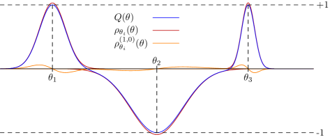
In the remainder of this section we show that our proposed construction yields a valid certificate if the conditions of Theorem 2.6 hold. In Section 3.3 we prove Lemma 3.2, which establishes that the interpolation equations have a unique solution and therefore $Q$ satisfies (3.1).

Lemma 3.2.

Under the assumptions of Theorem 2.6 there exist $\alpha,\beta\in\mathbb{R}^{k}$ which uniquely solve Equations 3.4 and 3.5.

In Section 3.4 we prove Lemma 3.3, which establishes that $Q$ satisfies (3.2). This completes the proof of Theorem 2.6.

Lemma 3.3.

Let $\alpha,\beta\in\mathbb{R}^{k}$ be the coefficients obtained in Lemma 3.2. Under the assumptions of Theorem 2.6 , the interpolating function $Q$ defined in (3.8) satisfies $|Q(\theta)|<1$ for $\theta\notin\Theta$.

3.3 Proof of Lemma 3.2

To simplify notation we define the $i$th normalized correlation and its derivatives by

$$\hat{\rho}_{\theta_{i}}^{(q,r)}(\theta):=\frac{\rho_{\theta_{i}}^{(q,r)}(\theta)}{\left\|\vec{\varphi}^{(q)}(\theta_{i})\right\|_{2}^{2}},$$ (3.10)

for $q=0,1$ and $r=0,1,2$, where $\rho_{\theta_{i}}^{(q,r)}$ is defined in Equation 2.1. Using this notation we have

$$Q(\theta) =\sum_{i=1}^{k}\alpha_{i}\rho_{\theta_{i}}(\theta)+\beta_{i}\frac{\rho^{(1,0)}_{\theta_{i}}(\theta)}{\rho_{\theta_{i}}^{(1,1)}(\theta_{i})}$$ (3.11)

$$=\sum_{i=1}^{k}\alpha_{i}\hat{\rho}_{\theta_{i}}(\theta)+\beta_{i}\hat{\rho}_{\theta_{i}}^{(1,0)}(\theta).$$ (3.12)

To prove Lemma 3.2 we establish the following stronger result, which also gives useful bounds on $\alpha$ and $\beta$. Throughout we assume that $\rho$ satisfies Conditions 2.1, 2.2 and 2.3 and (2.11) with parameters $\gamma$, $C$, $N$, $D$, and $\sigma$, and that $\Theta$ has separation $\Delta$.

Lemma 3.4.

Let $s:=2e^{-\Delta}/(1-e^{-\Delta})$. If $\Delta>\log(1+2(C_{0,0}+C_{1,1}))$ then there are $\alpha,\beta\in\mathbb{R}^{k}$ which uniquely solve equations (3.4) and (3.5). Furthermore, we have

$$\left\|\alpha\right\|_{\infty}\leq\frac{1-C_{1,1}s}{1-(C_{0,0}+C_{1,1})s},\quad\left\|\beta\right\|_{\infty}\leq\frac{C_{0,1}s}{1-(C_{0,0}+C_{1,1})s},\quad\text{and}\quad 1-\left\|\alpha-\xi\right\|_{\infty}\geq\frac{1-(2C_{0,0}+C_{1,1})s}{1-(C_{0,0}+C_{1,1})s}.$$

To prove Lemma 3.4 we begin by rewriting Equations (3.4) and (3.5) in block matrix-vector form for the $Q$ function defined in Equation 3.8:

$$\begin{bmatrix}\mathcal{I}+P^{(0,0)}&P^{(1,0)}\\ P^{(0,1)}&\mathcal{I}+P^{(1,1)}\end{bmatrix}\begin{bmatrix}\alpha\\ \beta\end{bmatrix}=\begin{bmatrix}\xi\\ 0\end{bmatrix},$$ (3.13)

where $\mathcal{I}\in\mathbb{R}^{{k}\times{k}}$ is the identity matrix, and $P^{(q,r)}\in\mathbb{R}^{{k}\times{k}}$ satisfies

$$P^{(q,r)}_{ij}=\hat{\rho}_{\theta_{j}}^{(q,r)}(\theta_{i})$$ (3.14)

for $i\neq j$ and $P^{(q,r)}_{ii}=0$. To see why $P_{ii}^{(1,0)}=0$ agrees with equations (3.4) and (3.5), note that

$$\hat{\rho}_{\theta_{i}}^{(1,0)}(\theta_{i})=\frac{\vec{\varphi}^{(1)}(\theta_{i})^{T}\vec{\varphi}(\theta_{i})}{\left\|\vec{\varphi}^{(1)}(\theta_{i})\right\|_{2}^{2}}=0.$$ (3.15)

The atoms are normalized– $\left\|\vec{\varphi}(\theta)\right\|_{2}=1$ for all $\theta$– which implies

$$0=\frac{d}{d\theta}\left\|\vec{\varphi}(\theta)\right\|_{2}^{2}=2\vec{\varphi}^{(1)}(\theta)^{T}\vec{\varphi}(\theta).$$

For the same reason it follows that $\hat{\rho}_{\theta_{i}}^{(0,1)}(\theta_{i})=0$.

Our plan is to bound the norm of each $P^{(q,r)}$. If these norms are sufficiently small then the matrix in Equation 3.13 is nearly the identity, and the desired result follows from a linear-algebraic argument. Define $\epsilon_{i}^{(q,r)}(\theta)$ by

$$\epsilon_{i}^{(q,r)}(\theta):=\sum_{j\neq i}|\hat{\rho}_{\theta_{j}}^{(q,r)}(\theta)|,$$ (3.16)

where $q=0,1$ and $r=0,1,2$. Here we think of $\theta$ as a point close to $\theta_{i}$, so $\epsilon_{i}^{(q,r)}(\theta)$ captures the cumulative correlation from the other, more distant elements of $\Theta$. We expect $\epsilon_{i}^{(q,r)}(\theta)$ to be small when $\rho$ has sufficient decay and $\Theta$ is well separated. For a matrix $A$ let $\left\|A\right\|_{\infty}$ denote the infinity-norm defined by

$$\left\|A\right\|_{\infty}:=\sup_{\left\|x\right\|_{\infty}=1}\left\|Ax\right\|_{\infty}.$$ (3.17)

$\left\|A\right\|_{\infty}$ equals the maximum sum of absolute values in any row of $A$. We have

$$\|P^{(q,r)}\|_{\infty}=\epsilon^{(q,r)}:=\max_{i\in\{1,\ldots,{k}\}}\epsilon_{i}^{(q,r)}(\theta_{i}).$$ (3.18)

The following lemma shows that equation (3.13) is invertible when $\epsilon^{(q,r)}$ is sufficiently bounded.

Lemma 3.5 (Proof in Appendix B).

Suppose

$$\epsilon^{(1,1)} <1\quad\text{and}$$ (3.19)

$$c:=\epsilon^{(0,0)}+\frac{\epsilon^{(1,0)}\epsilon^{(0,1)}}{1-\epsilon^{(1,1)}} <1.$$ (3.20)

Then the matrix in (3.13) is invertible and

$$\|\alpha\|_{\infty} \leq\frac{1}{1-c}$$ (3.21)

$$\|\beta\|_{\infty} \leq\frac{\epsilon^{(0,1)}/(1-\epsilon^{(1,1)})}{1-c}$$ (3.22)

$$\|\alpha-\xi\|_{\infty} \leq\frac{c}{1-c}.$$ (3.23)

To apply Lemma 3.5 we must first bound $\epsilon^{(q,r)}$ for $q,r\in\{0,1\}$. By the decay and separation conditions (Condition 2.3 and Definition 2.5), $\theta_{j}$ lies in the exponentially decaying tail of $\rho_{\theta_{i}}$, for $i\neq j$. This gives

$$\epsilon_{i}^{(q,r)}(\theta_{i}) =\sum_{j\neq i}|\hat{\rho}_{\theta_{j}}^{(q,r)}(\theta_{i})|$$ (3.24)

$$\leq C_{q,r}\sum_{\theta_{j}>\theta_{i}}\exp\left(-d(\theta_{i},\theta_{j})\right)+C_{q,r}\sum_{\theta_{j}<\theta_{i}}\exp\left(-d(\theta_{i},\theta_{j})\right)$$ (3.25)

$$\leq 2C_{q,r}\sum_{k=1}^{\infty}\exp\left(-k\Delta\right)$$ (3.26)

$$=\frac{2C_{q,r}e^{-\Delta}}{1-e^{-\Delta}}=C_{q,r}s,$$ (3.27)

where $s:=2e^{-\Delta}/(1-e^{-\Delta})$ and the distance $d$ is defined in Definition 2.5. As this bound is independent of $i$, we have

$$\epsilon^{(q,r)}\leq C_{q,r}s$$ (3.28)

for $q,r\in\{0,1\}$. In terms of the conditions of Lemma 3.5, we obtain

$$c=\epsilon^{(0,0)}+\frac{\epsilon^{(1,0)}\epsilon^{(0,1)}}{1-\epsilon^{(1,1)}}\leq C_{0,0}s+\frac{C_{1,0}C_{0,1}s^{2}}{1-C_{1,1}s}=\frac{C_{0,0}s+(C_{1,0}C_{0,1}-C_{0,0}C_{1,1})s^{2}}{1-C_{1,1}s}=\frac{C_{0,0}s}{1-C_{1,1}s},$$ (3.29)

assuming Equation 2.11 ($C_{1,0}C_{0,1}=C_{0,0}C_{1,1}$) holds. Thus we have $c<1$, as required by (3.20), when $s<\frac{1}{C_{0,0}+C_{1,1}}$. Using this, we can find conditions on $\Delta$ so that the hypotheses of Lemma 3.5 hold. If $\Delta>\log(1+\kappa)$ for some $\kappa>0$ then, using that $f(x)=e^{-x}/(1-e^{-x})$ is decreasing for $x>0$, we have

$$\frac{s}{2}=\frac{e^{-\Delta}}{1-e^{-\Delta}}<\frac{1/(1+\kappa)}{1-1/(1+\kappa)}=\frac{1}{\kappa}.$$ (3.30)

Letting $\kappa=2C_{1,1}$ this shows that $\Delta>\log(1+2C_{1,1})$ implies

$$\epsilon^{(1,1)}\leq C_{1,1}s=2C_{1,1}\frac{s}{2}<2C_{1,1}\frac{1}{2C_{1,1}}=1,$$ (3.31)

giving (3.19). For condition (3.20) we let $\kappa=2(C_{0,0}+C_{1,1})$. Then (3.30) shows that $\Delta>\log(1+2(C_{0,0}+C_{1,1}))$ implies

$$s=2\frac{s}{2}<2\frac{1}{2(C_{0,0}+C_{1,1})}=\frac{1}{C_{0,0}+C_{1,1}}$$ (3.32)

as required. Thus when $\Delta>\log(1+2(C_{0,0}+C_{1,1}))$ both conditions of Lemma 3.5 hold. By plugging (3.28) and (3.29) into the bounds of Lemma 3.5 we obtain Lemma 3.4. This completes the proof of Lemma 3.2.

3.4 Proof of Lemma 3.3

Lemma 3.2 implies that we can solve (3.4) and (3.5) for $\alpha$ and $\beta$ and then obtain $Q$ via (3.8). To prove Lemma 3.3 we must show that $|Q(\theta)|<1$ for $\theta\in\Theta^{c}$. This is accomplished in two steps. We first show that $|Q(\theta)|<1$ for $\theta$ that are not in the near region of any $\rho_{\theta_{i}}$, $i=1,\ldots,k$. Secondly, we show that for any $\theta$ in the near region of some $\rho_{\theta_{i}}$ we have $Q^{(2)}(\theta)<0$, where we assume $\xi_{i}=1$ without loss of generality. This proves that $Q$ has a local maximum at $\theta_{i}$, and is smaller than one nearby.

To bound $Q$ and $Q^{(2)}$ we apply the triangle inequality to (3.8), obtaining the following lemma.

Lemma 3.6.

Fix $\theta_{i}\in\Theta$ and let $Q$ be defined as in (3.8). For all $\theta\in\mathbb{R}$

$$|Q(\theta)|\leq\|\alpha\|_{\infty}|\hat{\rho}_{\theta_{i}}(\theta)|+\|\beta\|_{\infty}|\hat{\rho}_{\theta_{i}}^{(1,0)}(\theta)|+\|\alpha\|_{\infty}\epsilon_{i}^{(0,0)}(\theta)+\|\beta\|_{\infty}\epsilon_{i}^{(1,0)}(\theta).$$ (3.33)

If $\hat{\rho}_{\theta_{i}}^{(0,2)}(\theta)\leq 0$ and $\xi\in\{-1,+1\}^{k}$ is the sign pattern interpolated by $Q$ then

$$Q^{(2)}(\theta)\leq(1-\left\|\alpha-\xi\right\|_{\infty})\hat{\rho}_{\theta_{i}}^{(0,2)}(\theta)+\|\beta\|_{\infty}|\hat{\rho}_{\theta_{i}}^{(1,2)}(\theta)|+\|\alpha\|_{\infty}\epsilon_{i}^{(0,2)}(\theta)+\|\beta\|_{\infty}\epsilon_{i}^{(1,2)}(\theta).$$ (3.34)

In the next lemma we show that the separation conditions in Definition 2.5 ensure that the support does not cluster together. We assume that $\theta_{1}<\theta_{2}<\cdots<\theta_{|\Theta|}$.

Lemma 3.7 (Proof in Appendix C).

Fix $\theta_{i}\in\Theta$ and let $\theta>\theta_{i}$. If $i\leq k-1$, assume that

$$\frac{\theta-D_{i}^{+}}{\sigma_{i}}\leq\frac{D_{i+1}^{-}-\theta}{\sigma_{i+1}}.$$ (3.35)

Then

$$\frac{D_{j}^{-}-\theta}{\sigma_{j}} \geq\frac{\Delta}{2} j=i+1$$ if , (3.36)

$$\frac{D_{j}^{-}-\theta}{\sigma_{j}} \geq\Delta(j-(i+1)) j>i+1$$ if , (3.37)

$$\frac{\theta-D_{j}^{+}}{\sigma_{j}} \geq\Delta(i-j) j<i$$ if , (3.38)

where $\Delta$ is defined in Definition 2.5, as long as Conditions 2.1, 2.2 and 2.3 and (2.11) hold.

Inequality (3.35) implies that $\theta_{i}$ is the closest element of $\Theta$ to $\theta$, if we use the generalized distance normalized by $\sigma$.

Bounding $|Q(\theta)|$ Outside the Near Region

Our goal is to bound $|Q(\theta)|$ for $\theta\in\mathbb{R}$ that are not in the near region of any $\rho_{\theta_{i}}$. We can assume, flipping the axis if necessary, that the conditions of Lemma 3.7 hold for the $\theta_{i}$ closest to $\theta$ and that $\theta\geq N_{i}^{+}$ (recall that $N_{i}^{+}=\theta_{i}+N_{i}$ is the boundary of the near region of $\rho_{\theta_{i}}$). Then $\theta$ lies in the exponentially decaying tail of $\rho_{\theta_{j}}$ for $j\neq i$, so that

$$\epsilon_{i}^{(q,r)}(\theta) =\sum_{j\neq i}\hat{\rho}_{\theta_{j}}^{(q,r)}(\theta)$$ (3.39)

$$\leq C_{q,r}\exp(-(D_{i+1}^{-}-\theta)/\sigma_{i+1})$$

$$\quad+\sum_{j<i}C_{q,r}\exp(-(\theta-D_{j}^{+})/\sigma_{j})+\sum_{j>i+1}C_{q,r}\exp(-(D_{j}^{-}-\theta)/\sigma_{j})$$ (3.40)

$$\leq C_{q,r}e^{-\Delta/2}+2C_{q,r}\sum_{k=1}^{\infty}e^{-k\Delta}$$ (3.41)

$$=C_{q,r}(x+s),$$ (3.42)

where $x=e^{-\Delta/2}$ and $s$ is defined in Lemma 3.4. Plugging this into (3.33) and combining with Lemma 3.4 yields

$$|Q(\theta)| \leq\frac{1-C_{1,1}s}{1-(C_{0,0}+C_{1,1})s}\left(|\hat{\rho}_{\theta_{i}}(\theta)|+C_{0,0}(x+s)\right)$$

$$\qquad+\frac{C_{0,1}s}{1-(C_{0,0}+C_{1,1})s}\left(|\hat{\rho}_{\theta_{i}}^{(1,0)}(\theta)|+C_{1,0}(x+s)\right)$$ (3.43)

$$\leq\frac{1-C_{1,1}s}{1-(C_{0,0}+C_{1,1})s}\left(\gamma_{2}+C_{0,0}(x+s)\right)+\frac{C_{0,1}s}{1-(C_{0,0}+C_{1,1})s}\left(\gamma_{3}+C_{1,0}(x+s)\right).$$ (3.44)

Solving for $|Q(\theta)|<1$ we obtain

$$\left(1-C_{1,1}s\right)\left(\gamma_{2}+C_{0,0}(x+s)\right)+\left(C_{0,1}s\right)\left(\gamma_{3}+C_{1,0}(x+s)\right)<1-(C_{0,0}+C_{1,1})s.$$ (3.45)

Isolating $s$ and $x$,

$$s(2C_{0,0}+C_{1,1}-C_{1,1}\gamma_{2}+C_{0,1}\gamma_{3})+xC_{0,0}<1-\gamma_{2},$$ (3.46)

where we apply Equation 2.11 ($C_{1,0}C_{0,1}=C_{0,0}C_{1,1}$) to cancel terms. Since $s=\frac{2x^{2}}{1-x^{2}}$ we obtain the inequality

$$\frac{2x^{2}}{1-x^{2}}a+xb<c$$ (3.47)

where $a:=2C_{0,0}+C_{1,1}-C_{1,1}\gamma_{2}+C_{0,1}\gamma_{3}>0$, $b:=C_{0,0}$, and $c:=1-\gamma_{2}>0$. The following lemma shows that this inequality is satisfied by our assumptions, completing this part of the proof.

Lemma 3.8 (Proof in Appendix D).

Let $a,b,c,\Delta>0$, and $x:=e^{-\Delta/2}$. Then the inequality

$$\frac{2x^{2}}{1-x^{2}}a+xb<c$$ (3.48)

is satisfied when

$$\Delta>2\log\left(\frac{2(2a+c)}{-b+\sqrt{b^{2}+4(2a+c)c}}\right).$$ (3.49)

Bounding $Q^{(2)}(\theta)$ in the Near Region

For the final part of the proof we must prove $Q^{(2)}(\theta)<0$ for $\theta$ in the near region of some $\theta_{i}$ with $\xi_{i}=1$. Since the interpolation equations (3.4) and (3.5) guarantee that $Q(\theta_{i})=1$, strict concavity implies that $Q$ has a unique maximum on $[N_{i}^{-},N_{i}^{+}]$ thus establishing that $Q(\theta)<1$ for $\theta\in[N_{i}^{-},N_{i}^{+}]\setminus\{\theta_{i}\}$. We cannot have $Q(\theta)\leq-1$ on the near region since we already showed that $|Q(\theta)|<1$ outside the near region. We can assume, without loss of generality, that the conditions of Lemma 3.7 hold for some $i$ and that $\theta\leq N_{i}^{+}$. By the same argument used to obtain Equation 3.42, we have

$$\epsilon_{i}^{(q,r)}(\theta)\leq C_{q,r}(x+s).$$ (3.50)

Plugging this into (3.33) and applying Lemma 3.4 we obtain

$$Q^{(2)}(\theta) \leq\frac{1-(2C_{0,0}+C_{1,1})s}{1-(C_{0,0}+C_{1,1})s}\hat{\rho}_{\theta_{i}}^{(0,2)}(\theta)+\frac{1-C_{1,1}s}{1-(C_{0,0}+C_{1,1})s}\left(C_{0,2}(x+s)\right)$$

$$+\frac{C_{0,1}s}{1-(C_{0,0}+C_{1,1})s}\left(|\hat{\rho}_{\theta_{i}}^{(1,2)}(\theta)|+C_{1,2}(x+s)\right)$$ (3.51)

$$\leq\frac{1-(2C_{0,0}+C_{1,1})s}{1-(C_{0,0}+C_{1,1})s}\left(-\gamma_{0}\right)+\frac{1-C_{1,1}s}{1-(C_{0,0}+C_{1,1})s}\left(C_{0,2}(x+s)\right)$$

$$+\frac{C_{0,1}s}{1-(C_{0,0}+C_{1,1})s}\left(\gamma_{1}+C_{1,2}(x+s)\right),$$ (3.52)

where $\hat{\rho}_{\theta_{i}}^{(0,2)}(\theta)\leq 0$ by Condition 2.1. Solving for $Q^{(2)}(\theta)<0$ yields

$$-(1-(2C_{0,0}+C_{1,1})s)\gamma_{0}+(1-C_{1,1}s)C_{0,2}(x+s)+C_{0,1}s(\gamma_{1}+C_{1,2}(x+s))<0.$$ (3.53)

Grouping into terms involving $s$ and $x$ we obtain

$$s((2C_{0,0}+C_{1,1})\gamma_{0}+C_{0,2}+C_{0,1}\gamma_{1})+C_{0,2}x<\gamma_{0},$$ (3.54)

where we apply Equation 2.11 ($C_{0,1}C_{1,2}=C_{0,2}C_{1,1}$) to cancel terms. Letting $a:=(2C_{0,0}+C_{1,1})\gamma_{0}+C_{0,2}+C_{0,1}\gamma_{1}>0$, $b:=C_{0,2}$, and $c:=\gamma_{0}>0$ we obtain an inequality of the form (3.48). Applying Lemma 3.8 completes the proof.

Figure 16: Interpolation function $Q$ associated to a valid dual certificate for the electroencephalography brain-activity localization problem. The dual certificate is associated to a signal consisting of the three sources of brain activity shown in Figure 2. $Q$ interpolates the sign pattern of the signal, which equals +1 on $\theta_{1}$ and $\theta_{3}$, and -1 on $\theta_{2}$. The certificate is built using the multidimensional extension of our proposed interpolation technique described in Section 3.5.

3.5 Extensions to Higher Dimensions

In this section we briefly describe an extension of our dual certificate construction to settings where the parameter space has dimension $p>1$. We leave a more detailed analysis to future work. In higher dimensions, one can build the interpolating function $Q$ by setting

$$Q(\eta):=\sum_{i=1}^{k}\left[\alpha_{i}\rho_{\theta_{i}}(\eta)+\sum_{l=1}^{p}\beta_{i,l}\frac{\partial_{1,l}\,\rho_{\theta_{i}}(\eta)}{\left\|\partial_{l}\vec{\varphi}(\theta_{i})\right\|_{2}^{2}}\right],$$ (3.55)

where $\alpha\in\mathbb{R}^{k}$, $\beta\in\mathbb{R}^{k\times p}$, $\partial_{l}$ denotes the partial derivative with respect to the $l$th coordinate, and $\partial_{1,l}\rho_{\theta}(\eta)$ denotes the partial derivative of $\rho_{\theta}(\eta)$ with respect to the $l$th coordinate of $\theta$. The coefficients are chosen so that $Q$ satisfies the analog of the interpolation Equations 3.4 and 3.5,

$$Q(\theta_{i}) =\xi_{i},$$ (3.56)

$$\nabla Q(\theta_{i}) =0.$$ (3.57)

In Figure 16 we show an example of an interpolating function $Q$ for the electroencephalography brain-activity localization problem. The interpolating function is associated to the signal with three active sources of brain activity from Figure 2. To control $Q$ for problems with correlation decay, one can extend the correlation-decay conditions in Section 2.1 to higher dimensions by requiring analogous bounds on the first and second partial derivatives. For example, the local quadratic bound in Equation 2.2 becomes a bound on the eigenvalues of the Hessian of $\rho_{\theta}$. Similar conditions have been used in [14, 2] to obtain recovery guarantees for the super-resolution and deconvolution problems in two dimensions.

4 Numerical Experiments

4.1 Heat-source localization

Our theoretical results establish that convex programming yields exact recovery in parameter-estimation problems that have correlation decay. In this section we investigate this phenomenon numerically for a heat-source localization problem in one dimension. The heat sources are modeled as a collection of point sources,

$$\mu:=\sum_{\theta_{i}\in\Theta}c_{i}\delta_{\theta_{i}},$$ (4.1)

where $\Theta$ is a finite number of points in the unit interval and $c_{i}\in\mathbb{R}$ for $i=1,\ldots,k$.

The heat $u(\theta,t)$ at position $\theta$ and time $t$ is assumed to evolve following the heat equation with Neumann boundary conditions (see e.g. [57]),

$$\frac{\partial}{\partial t}u(\theta,t) =\frac{\partial}{\partial\theta}\left(c(\theta)\frac{\partial}{\partial\theta}u(\theta,t)\right),$$ (4.2)

$$\frac{\partial}{\partial\theta}u(-0.5,t) =\frac{\partial}{\partial\theta}u(0.5,t)=0$$ (4.3)

on the unit interval, where $c(\theta)$ represents the conductivity of the medium at $\theta$ (see Figure 17). The data are heat measurements $u(j,T)$, where $j$ is sampled on a regular grid of 100 points at a fixed time $T:=10^{-4}$. Our goal is to recover the initial heat distribution at $t=0$ represented by the heat sources $\mu$. This is an SNL problem where $\vec{\varphi}(\theta)$ corresponds to the measurements caused by a source located at $\theta$.

Figure 17: The conductivity function $c(\theta)$ used in the experiment described in Section 4.1. Heat diffuses faster in the central region, where the conductivity is higher.

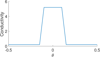
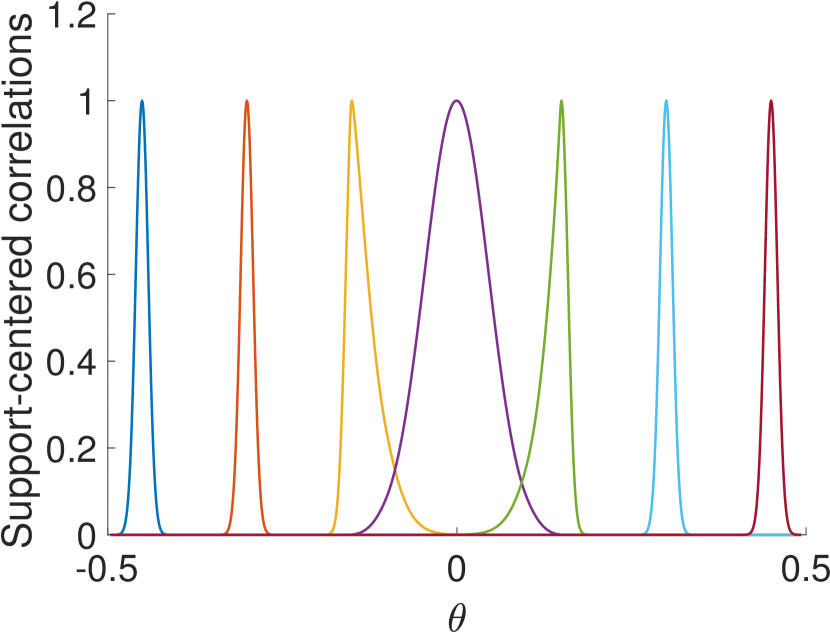
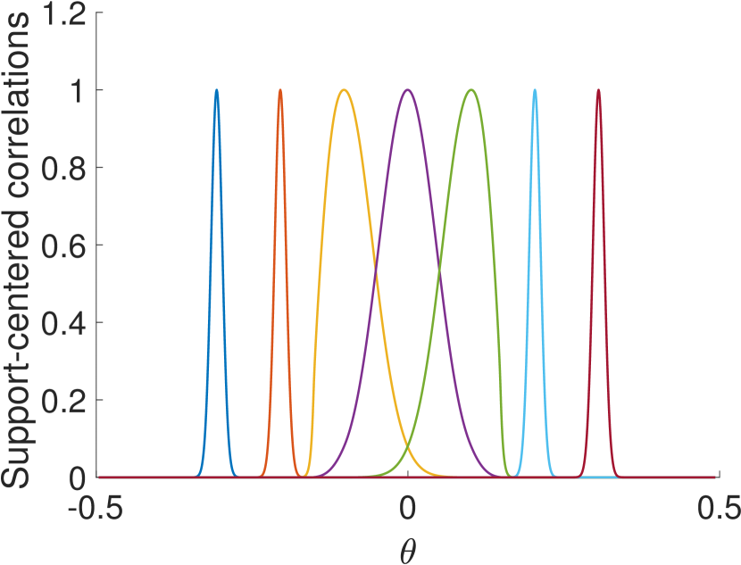
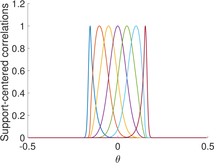
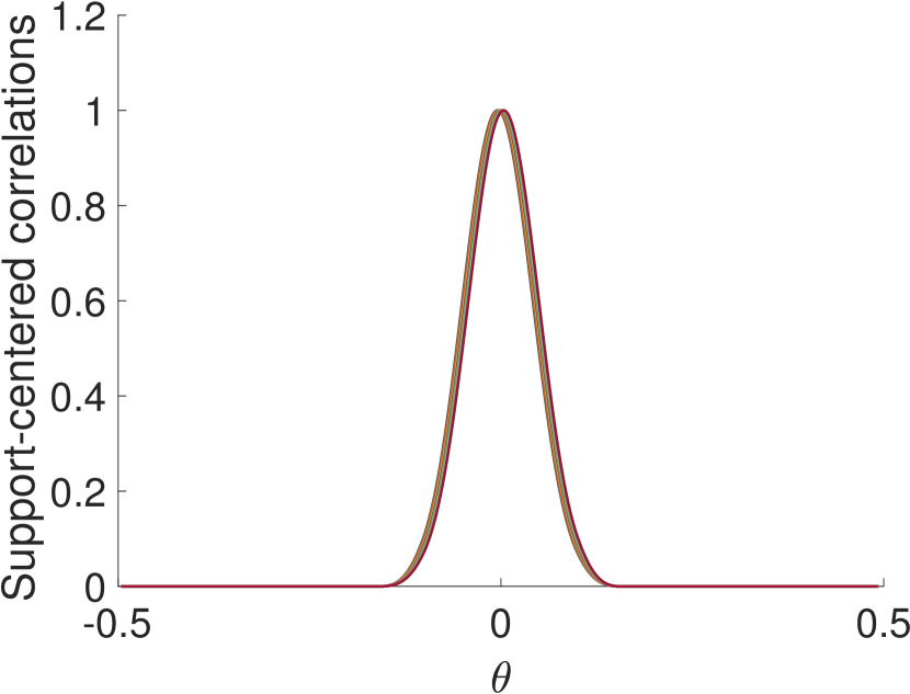
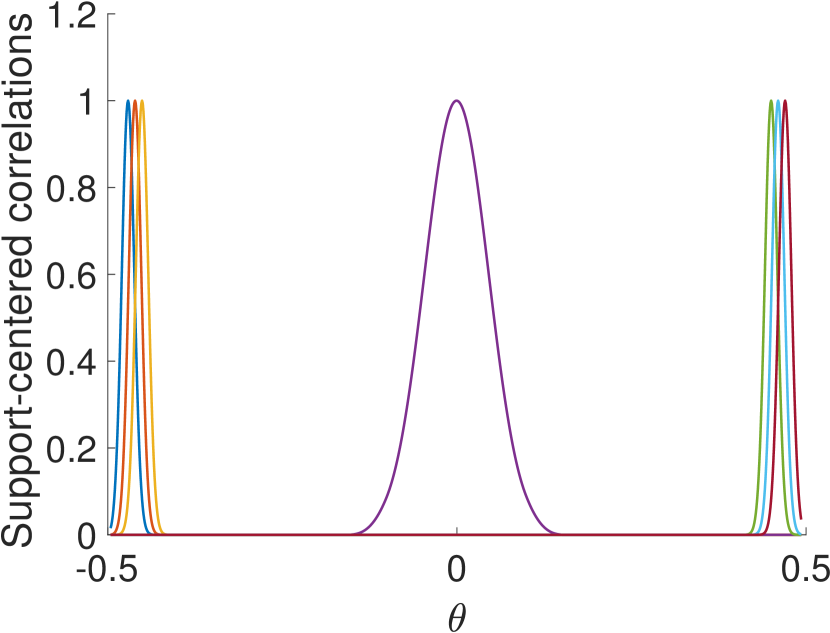
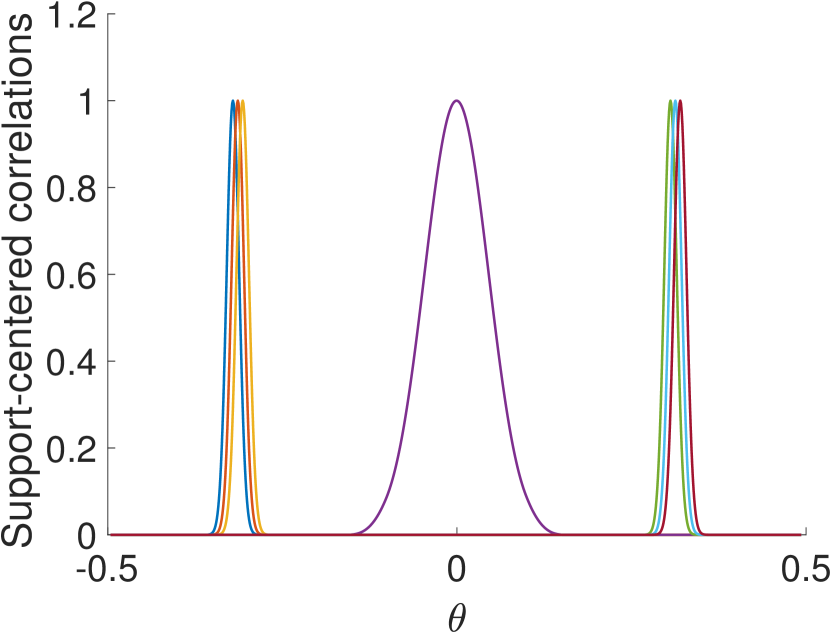
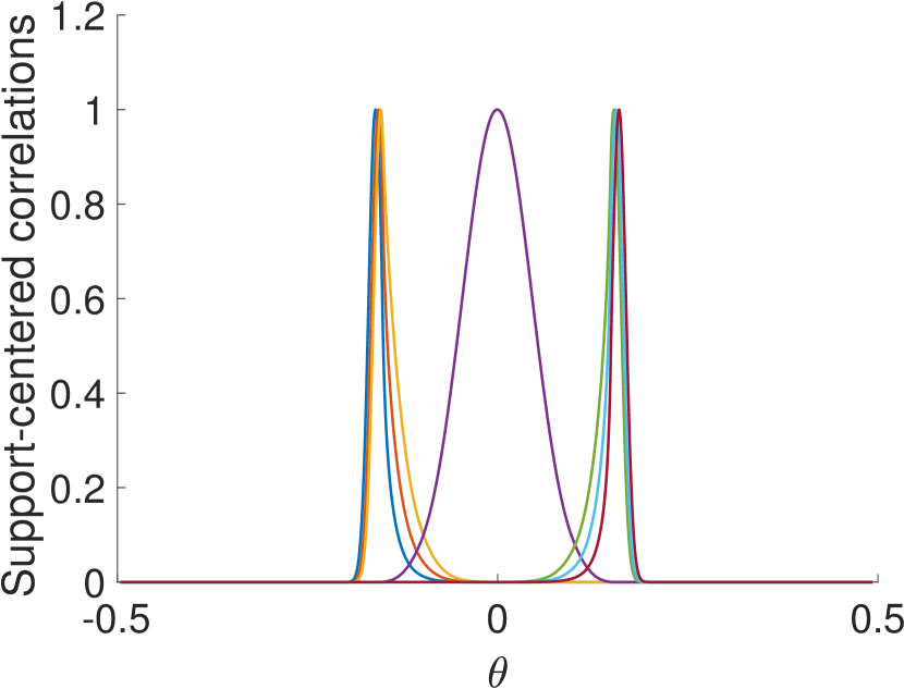
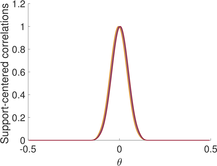
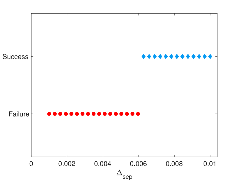
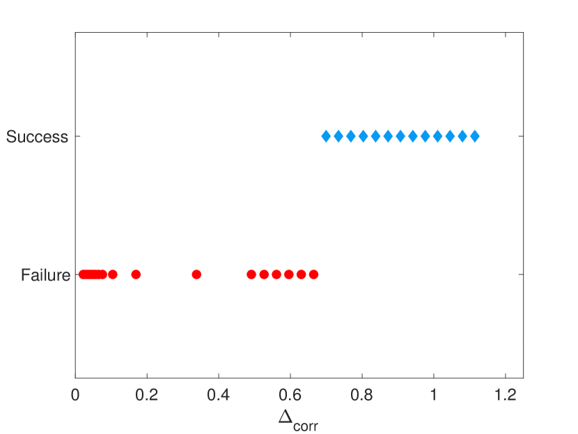
If the conductivity is constant, then $\vec{\varphi}(\theta)$ has a Gaussian-like shape with fixed width sampled on the measurement grid, and the correlation function $\rho_{\theta}$ is also shaped like a Gaussian with fixed width. In this example, the conductivity varies (see Figure 17), which results in correlations that are still mostly Gaussian-like but have very different widths (see Figure 18). The measurement operator therefore has nonuniform correlation decay properties. According to the theory presented in Section 2.3, we expect convex programming to recover the heat-source location as long as they are separated by a minimum separation that takes into account the structure of the correlation decay. To verify whether this is the case we consider two different separation measures. The first just measures the minimum separation between the sources,

$$\Delta_{\operatorname{sep}}:=\min_{i\neq j}|\theta_{i}-\theta_{j}|.$$ (4.4)

The second takes into account the correlation function of the SNL problem,

$$\Delta_{\operatorname{corr}}:=\min_{i\neq j}\frac{|\theta_{i}-\theta_{j}|}{\max(\sigma_{i},\sigma_{j})}.$$ (4.5)

where $\sigma_{i}$, $1\leq i\leq k$, is the standard deviation of the best Gaussian upper bound on the correlation function centered at $\theta_{i}$,

$$\sigma_{i}:=\inf\{s>0\mid\rho_{\theta_{i}}(\theta)<e^{-(\theta_{i}-\theta)^{2}/(2s^{2})}~{}\text{for all $\theta$.}\}$$ (4.6)

	Dilation Factor
	$1$	$0.68$	$0.34$	$0.01$
Uniform
Clustered

Figure 18: Examples of the correlation functions $\rho_{\theta_{1}},\ldots,\rho_{\theta_{7}}$ for heat sources with different separations and configurations. The sources used in the top row of figures are uniformly spaced on the unit interval. The heat sources in the bottom row have one central source, and two clusters of three sources located at the ends. From left to right the supports are dilated by different factors. This reduces the separation between the heat sources but maintains their relative position.

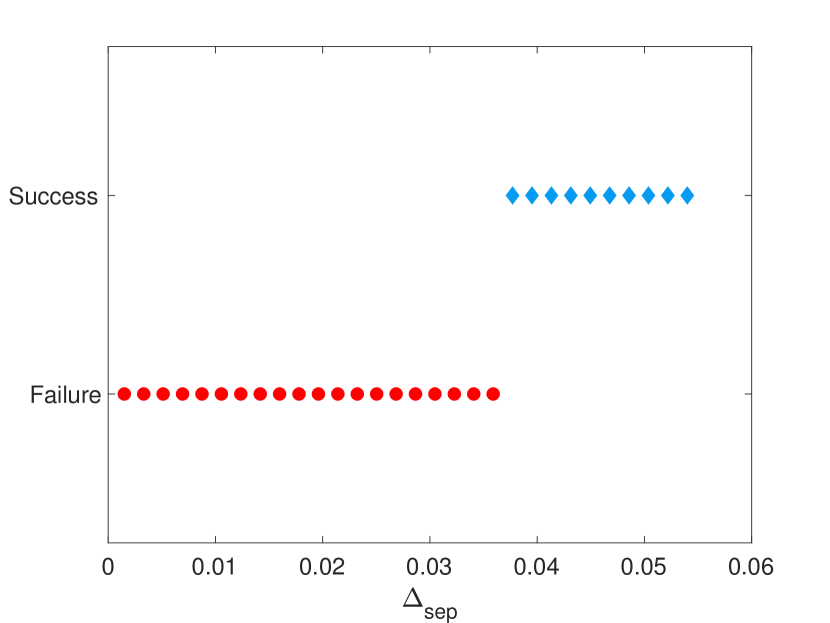
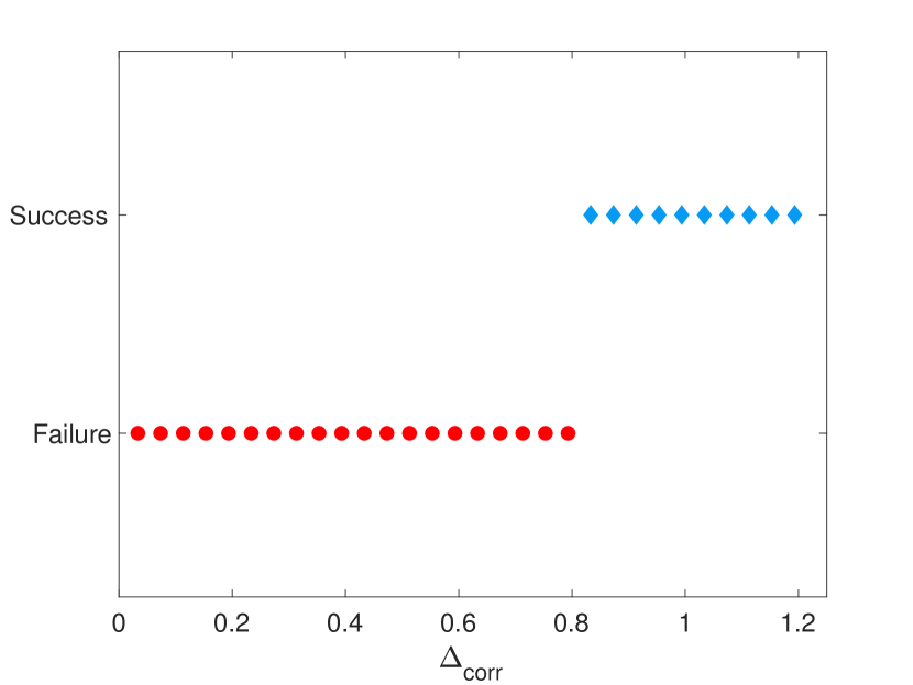
The question is which of these separations characterizes the performance of the convex-programming approach more accurately. We consider two different heat-source configurations: one where the sources are uniformly spaced and another where they are clustered, as depicted in Figure 18. In the clustered configuration, groups of spikes are placed in regions of low conductivity where each $\rho_{\theta_{i}}$ exhibits sharp decay. This creates a noticeable discrepancy between the two measures of separation. We expect exact recovery to occur for much smaller values of $\Delta_{\operatorname{sep}}$ in the clustered case than it does in the uniform case since it doesn’t account for the correlation decay. In contrast, we expect $\Delta_{\operatorname{corr}}$ to have similar thresholds for exact recovery in both cases, as it captures the inherent difficulty in the problem. To recover these sources we solve the discretized $\ell_{1}$-norm minimization problem described in Section 2.5 using CVX [47]. The measurement matrix is computed by solving the differential equation on a grid of $10^{3}$ points in the parameter space.

	$\Delta_{\operatorname{sep}}$	$\Delta_{\operatorname{corr}}$
Uniform
Clustered

Figure 19: The figure shows the performance of heat-source localization based on convex programming for the experiment described in Section 4.1. The upper row shows the result for sources with uniformly spaced supports, whereas the bottom row shows results for sources with clustered supports (see Figure 18). The left column plots the results with respect to the minimum separation $\Delta_{\operatorname{sep}}$. The right column plots the results in terms of the correlation-aware separation $\Delta_{\operatorname{corr}}$. Recovery succeeds if the relative $\ell_{2}$-norm recovery error is smaller than $3\cdot 10^{-5}$. All failures have an absolute error above $9\cdot 10^{-3}$, and most have errors above 1. For comparison the $\ell_{2}$ norm of the true signal equals $\sqrt{7}$ ($\approx 2.65$) in all cases.

Figure 19 shows the results. For both types of support, we observe that exact recovery occurs as long as the minimum separation $\Delta_{\operatorname{sep}}$ between sources is larger than a certain value. However, this value is very different for the two types of support. It is much smaller for the clustered support. Intuitively, this is due to the fact that the clustered sources are mostly located in the region where the conductivity is lower, and consequently the correlation decay is much faster. Our theory suggests that exact recovery will occur at smaller separations for such configurations, which is what we observe. Quantifying separation using $\Delta_{\operatorname{corr}}$ accounts for the variation in correlation decay, resulting in a similar phase transition for both types of support. This is consistent with the theory for SNL problems with nonuniform correlation decay developed in Section 2.3.

4.2 Estimation of Brain Activity via Electroencephalography

In this section we consider the SNL problem of brain-activity localization from electroencephalography (EEG) data. Areas of focalized brain activity are usually known as sources. In EEG, as well as in magnetoencephalography, sources are usually modeled using electric dipoles, represented mathematically as point sources or Dirac measures at the corresponding locations [1]. EEG measurements are samples of the electric potential on the surface of the head obtained using an array of electrodes. The mapping from the source positions and amplitudes to the EEG data is governed by Poisson’s equation. For a fixed model of the head geometry– obtained for example from 3D images acquired using magnetic-resonance imaging– the mapping can be computed by solving the differential equation numerically. By linearity, this corresponds to an SNL model where $\theta$ represents the position of a dipole and $\varphi_{t}\left(\theta\right)$ is the value of the corresponding electrical potential at a location $t$ of the scalp.

To simulate realistic EEG data with associated ground-truth source positions, we use Brainstorm [86], an open-source software for the analysis of EEG and other electrophysiological recordings. We use template ICBM152, which is a nonlinear average of 152 3D magnetic-resonance image scans [41], to model the geometry of the brain and head. The sources are modeled as electrical dipoles situated on the cortical surface, discretized as a tesselated grid with 15,000 points. The orientation of the dipoles is assumed to be perpendicular to the cortex. The data-acquisition sensor array has 256 channels (HydroCel GSN, EGI). The data corresponding to each point on the grid are simulated numerically using the open-source software OpenMEEG [46]. The computation assumes realistic electrical properties for the brain, skull and scalp. As a result, we obtain a $256\times 15,000$ measurement operator that can be used to generate data corresponding to different combinations of sources. Figure 2 shows three examples.

The correlation structure of the EEG linear measurement operator is depicted in Figure 6. The complex geometric structure of the folds in cortex induce an intricate correlation structure close to the source location. However, the correlation presents a clear correlation decay; points that are far enough from the source have low correlation values. Our theoretical results consequently suggest that $\ell_{1}$-norm minimization should succeed in recovering superpositions of sources that are sufficiently separated. This is supported by the fact that for such superpositions, we can build valid dual certificates as illustrated in Figure 16.

Best case	Worst case

Figure 20: Result of the brain-source localization experiment described in Section 4.2. The horizontal axis indicates the distance between the sources. In the left image success is declared if the three sources are accurately recovered for any pattern of positive and negative amplitudes. In the right image success is declared if the sources are recovered for all patterns of positive and negative amplitudes. Recovery succeeds if the relative $\ell_{2}$-norm recovery error is smaller than $10^{-4}$. All failures have an absolute error above $1.18$. For comparison the $\ell_{2}$ norm of the true signal equals $\sqrt{3}$ ($\approx 1.73$) in all cases.

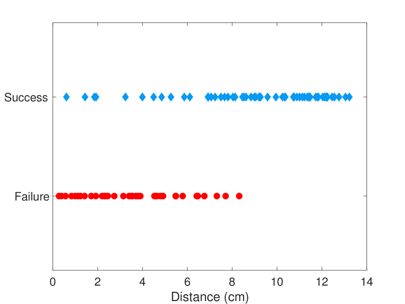
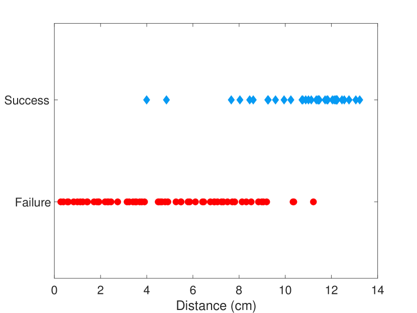
In order to test our hypothesis, we randomly choose superpositions of three sources located at approximately the same distance from each other, for a range of distances. For each superposition we generate 8 different measurement vectors by assigning every possible combination of positive and negative unit-norm amplitudes to each source. We then estimate the source locations by solving an $\ell_{1}$-norm minimization problem with equality constraints using CVX [47]. Figure 20 shows the results. When the separation is sufficiently large, exact recovery indeed occurs for all possible patterns of positive and negative amplitudes, as expected from our theoretical analysis. As the separation decreases, recovery fails for some of the patterns, as shown in the image on the right.

5 Conclusion and Future Work

In this work, we establish that deterministic SNL problems can be solved via a tractable convex optimization program, as long as the parameters have a minimum separation in the parameter space with respect to the correlation structure of the measurement operator. As mentioned in Sections 2.4, our results can be used to establish some robustness guarantees at low-noise levels in terms of support recovery. Deriving more precise stability analysis in the spirit of [56] is an interesting research direction. Another interesting open problem is characterizing the performance of reweighting techniques, which are commonly applied in practice to enhance solutions obtained from $\ell_{1}$-norm minimization [21, 90].

A drawback of the sparse-recovery framework discussed in this paper is computational complexity: for SNL problems in two or three dimensions it is very computationally expensive to solve $\ell_{1}$-norm minimization problems, even if we discretize the domain. In the last few years, algorithms that minimize nonconvex cost functions directly via gradient descent have been shown to provable succeed in solving underdetermined inverse problems involving randomized measurements [16, 59]. As illustrated in Figure 3, nonlinear least-squares cost functions associated to deterministic SNL problems often have non-optimal local minima. An intriguing question is how to design cost functions for deterministic SNL problems that can be tackled directly by descent methods.

Another computationally efficient alternative is to perform recovery using machine learning. Recent works suggest calibrating a feedforward network to output the model parameters using a training set of examples, with applications in point-source deconvolution [9] and super-resolution of line spectra [54]. Understanding under what conditions such techniques can be expected to yield accurate estimates is a challenging question for future research.

Acknowledgements

B.B. is supported by the MacCracken Fellowship, and the Isaac Barkey and Ernesto Yhap Fellowship. C.P. is supported by NIH award NEI-R01-EY025673. C.F. is supported by NSF award DMS-1616340.

Throughout the appendix, we assume there is some compact interval $I\subset\mathbb{R}$ containing the support $\Theta$ of the true measure $\mu$. In problem (1.8), the variable $\tilde{\mu}$ takes values in the set of finite signed Borel measures supported on $I$.

Appendix A Proof of Proposition 3.1

The following proof is standard, but given here for completeness.

.

Let $\nu$ be feasible for problem (1.8) and define $h=\nu-\mu$. By taking the Lebesgue decomposition of $h$ with respect to $|\mu|$ we can write

$$h=h_{\Theta}+h_{\Theta^{c}},$$ (A.1)

where $h_{\Theta}$ is absolutely continuous with respect to $|\mu|$, and $h_{\Theta^{c}}$, $|\mu|$ are mutually singular. In other words, the support of $h_{\Theta}$ is contained in $\Theta$, and $h_{\Theta^{c}}(\Theta)=0$. This allows us to write

$$h_{\Theta}=\sum_{t_{j}\in T}b_{j}\delta_{t_{j}},$$ (A.2)

for some $b\in\mathbb{R}^{|\Theta|}$. Set $\xi:=\operatorname*{sign}(b)$, where we arbitrarily choose $\xi_{j}=\pm 1$ if $b_{j}=0$. By assumption there exists a corresponding $Q$ interpolating $\xi$ on $\Theta$. Since $\mu$ and $\nu$ are feasible for problem (1.8) we have $\int\varphi(\theta)\,dh(\theta)=0$. This implies

$$0=q^{T}\int\varphi(\theta)\,dh(\theta)\\ =\int Q(\theta)\,dh(\theta)\\ =\left\|h_{\Theta}\right\|_{\operatorname{TV}}+\int Q(\theta)\,dh_{\Theta^{c}}(\theta).$$ (A.3)

Applying the triangle inequality, we obtain

$$\left\|\nu\right\|_{\operatorname{TV}} =\left\|\mu+h_{\Theta}\right\|_{\operatorname{TV}}+\left\|h_{\Theta^{c}}\right\|_{\operatorname{TV}}$$ (Mutually Singular) (A.4)

$$\geq\left\|\mu\right\|_{\operatorname{TV}}+\left\|h_{\Theta^{c}}\right\|_{\operatorname{TV}}-\left\|h_{\Theta}\right\|_{\operatorname{TV}}$$ (Triangle Inequality) (A.5)

$$=\left\|\mu\right\|_{\operatorname{TV}}+\left\|h_{\Theta^{c}}\right\|_{\operatorname{TV}}+\int Q(\theta)\,dh_{\Theta^{c}}(\theta)$$ (Equation (A.3)) (A.6)

$$\geq\left\|\mu\right\|_{\operatorname{TV}} \text{($|Q(\theta)|\leq 1$)},$$ (A.7)

where the last inequality is strict if $\left\|h_{\Theta^{c}}\right\|_{\operatorname{TV}}>0$ since $|Q(\theta)|<1$ for $\theta\in\Theta^{c}$. This establishes that $\mu$ is optimal for problem (1.8), and that any other optimal solution must be supported on $\Theta$. Equation A.3 implies that any feasible solution supported on $\Theta$ must be equal to $\mu$ (since $\left\|h_{\Theta}\right\|_{\operatorname{TV}}=0$), completing the proof of uniqueness. ∎

Appendix B Proof of Lemma 3.5

.

For any matrix $A\in\mathbb{R}^{n\times n}$ such that $\left\|A\right\|_{\infty}<1$ the Neumann series $\sum_{j=0}^{\infty}A^{j}$ converges to $(\mathcal{I}-A)^{-1}$, which implies that $\mathcal{I}-A$ is invertible [77]. By the triangle inequality and the submultiplicativity of the $\infty$-norm, this gives

$$\|(\mathcal{I}-A)^{-1}\|_{\infty}\leq\sum_{j=0}^{\infty}\|A\|_{\infty}^{j}=\frac{1}{1-\|A\|_{\infty}}.$$ (B.1)

Setting $A=-P^{(1,1)}$ and applying $\|P^{(1,1)}\|_{\infty}=\epsilon^{(1,1)}<1$ proves $\mathcal{I}+P^{(1,1)}$ is invertible. Let $\mathcal{C}$ be the Schur complement of $\mathcal{I}+P^{(1,1)}$ in (3.13) so that

$$\mathcal{C}=\mathcal{I}+P^{(0,0)}-P^{(1,0)}(\mathcal{I}+P^{(1,1)})^{-1}P^{(0,1)}.$$ (B.2)

By the triangle inequality and (B.1) applied with $A=-P^{(1,1)}$ we obtain

$$\|\mathcal{I}-\mathcal{C}\|_{\infty}\leq\epsilon^{(0,0)}+\frac{\epsilon^{(1,0)}\epsilon^{(0,1)}}{1-\epsilon^{(1,1)}}=c<1,$$ (B.3)

proving $\mathcal{C}$ is invertible. As both $\mathcal{I}+P^{(1,1)}$ and its Schur complement $\mathcal{C}$ are invertible, the matrix in (3.13) is also invertible (see e.g. [99]), which establishes the first claim.

By applying blockwise Gaussian elimination we solve (3.13) in terms of $\mathcal{C}$ to obtain

$$\alpha =\mathcal{C}^{-1}\xi$$ (B.4)

$$\beta =-(\mathcal{I}+P^{(1,1)})^{-1}P^{(0,1)}\alpha.$$ (B.5)

Applying (B.1) and noting that $\left\|\xi\right\|_{\infty}=1$ we obtain the required bounds on $\left\|\alpha\right\|_{\infty}$ and $\left\|\beta\right\|_{\infty}$. Finally,

$$(\mathcal{I}-\mathcal{C})\alpha=\alpha-\xi,$$ (B.6)

which implies $\left\|\alpha-\xi\right\|_{\infty}\leq c\left\|\alpha\right\|_{\infty}$ and completes the proof. ∎

Appendix C Proof of Lemma 3.7

.

Throughout we use the fact that $\Theta$ having separation $\Delta>0$ (Definition 2.5) implies $D_{i}^{+}\leq D_{j}^{-}$ for $j>i$. When $i\leq k-1$, (3.35) implies that

$$\theta\leq\frac{\sigma_{i}D_{i+1}^{-}+\sigma_{i+1}D_{i}^{+}}{\sigma_{i}+\sigma_{i+1}},$$

where the righthand side is the $\sigma$-weighted average of $D_{i}^{+}$ and $D_{i+1}^{-}$. If $\theta\geq D_{i}^{+}$ this gives

$$\frac{D_{i+1}^{-}-\theta}{\sigma_{i+1}}\geq\frac{D_{i+1}^{-}-D_{i}^{+}}{\sigma_{i}+\sigma_{i+1}}\geq\frac{\max(\sigma_{i},\sigma_{i+1})\Delta}{\sigma_{i}+\sigma_{i+1}}\geq\frac{\Delta}{2}.$$

If $\theta<D_{i}^{+}$ then

$$\frac{D_{i+1}^{-}-\theta}{\sigma_{i+1}}>\frac{D_{i+1}^{-}-D_{i}^{+}}{\sigma_{i+1}}\geq\frac{D_{i+1}^{-}-D_{i}^{+}}{\max(\sigma_{i},\sigma_{i+1})}\geq\Delta>\frac{\Delta}{2},$$ (C.1)

by the separation conditions, proving (3.36). If $i+1<j\leq|\Theta|$ then $d(\theta_{i+1},\theta_{j})\geq\Delta(j-(i+1))$, so that

$$\frac{D_{j}^{-}-\theta}{\sigma_{j}}\geq\frac{D_{j}^{-}-D_{i+1}^{+}}{\sigma_{j}}\geq\frac{D_{j}^{-}-D_{i+1}^{+}}{\max(\sigma_{j},\sigma_{i+1})}\geq\Delta(j-(i+1)),$$ (C.2)

by the separation conditions applied to $\theta_{j}$ and $\theta_{i+1}$, which implies (3.37). Finally, if $j<i$ then

$$\frac{\theta-D_{j}^{+}}{\sigma_{j}}\geq\frac{D_{i}^{-}-D_{j}^{+}}{\sigma_{j}}\geq\frac{D_{i}^{-}-D_{j}^{+}}{\max(\sigma_{j},\sigma_{i})}\geq\Delta(i-j),$$ (C.3)

by the separation conditions applied to $\theta_{j}$ and $\theta_{i}$, which establishes (3.38). ∎

Appendix D Proof of Lemma 3.8

.

Multiplying through by $1-x^{2}$ (which is positive by assumption) in (3.48) we obtain

$$-x^{3}b+(2a+c)x^{2}+xb-c<0.$$ (D.1)

The above inequality is implied by the simpler quadratic inequality

$$(2a+c)x^{2}+xb-c<0,$$ (D.2)

where the omitted term $-x^{3}b$ is always negative. Since the inequality is satisfied for $x=0$ we obtain the condition

$$0<x<\frac{-b+\sqrt{b^{2}+4(2a+c)c}}{2(2a+c)}.$$ (D.3)

Translating this to a statement on $\Delta$ we obtain

$$\Delta>2\log\left(\frac{2(2a+c)}{-b+\sqrt{b^{2}+4(2a+c)c}}\right).$$ (D.4)

∎

References

- [1] S. Baillet, J. C. Mosher, and R. M. Leahy. Electromagnetic brain mapping. IEEE Signal processing magazine, 18(6):14–30, 2001.
- [2] T. Bendory, S. Dekel, and A. Feuer. Robust recovery of stream of pulses using convex optimization. Journal of Mathematical Analysis and Applications, 442(2):511–536, 2016.
- [3] B. Bernstein and C. Fernandez-Granda. Deconvolution of point sources: a sampling theorem and robustness guarantees. arXiv preprint arXiv:1707.00808, 2017.
- [4] N. Bertin, L. Daudet, V. Emiya, and R. Gribonval. Compressive sensing in acoustic imaging. In Compressed Sensing and its Applications, pages 169–192. Springer, 2015.
- [5] E. Betzig, G. H. Patterson, R. Sougrat, O. W. Lindwasser, S. Olenych, J. S. Bonifacino, M. W. Davidson, J. Lippincott-Schwartz, and H. F. Hess. Imaging intracellular fluorescent proteins at nanometer resolution. Science, 313(5793):1642–1645, 2006.
- [6] P. J. Bickel, Y. Ritov, and A. B. Tsybakov. Simultaneous analysis of lasso and {D}antzig selector. The Annals of Statistics, pages 1705–1732, 2009.
- [7] F. Bloch. Nuclear induction. Physical review, 70(7-8):460, 1946.
- [8] L. Borcea and I. Kocyigit. Resolution analysis of imaging with ell_1 optimization. SIAM Journal on Imaging Sciences, 8(4):3015–3050, 2015.
- [9] N. Boyd, E. Jonas, H. P. Babcock, and B. Recht. Deeploco: Fast 3d localization microscopy using neural networks. BioRxiv, page 267096, 2018.
- [10] N. Boyd, G. Schiebinger, and B. Recht. The alternating descent conditional gradient method for sparse inverse problems. SIAM Journal on Optimization, 27(2):616–639, 2017.
- [11] E. Candes and B. Recht. Exact matrix completion via convex optimization. Communications of the ACM, 55(6):111–119, 2012.
- [12] E. J. Candes. The restricted isometry property and its implications for compressed sensing. Comptes Rendus Mathematique, 346(9-10):589–592, 2008.
- [13] E. J. Candes, Y. C. Eldar, T. Strohmer, and V. Voroninski. Phase retrieval via matrix completion. SIAM review, 57(2):225–251, 2015.
- [14] E. J. Candès and C. Fernandez-Granda. Towards a mathematical theory of super-resolution. Communications on Pure and Applied Mathematics, 67(6):906–956.
- [15] E. J. Candès and C. Fernandez-Granda. Super-resolution from noisy data. Journal of Fourier Analysis and Applications, 19(6):1229–1254, 2013.
- [16] E. J. Candes, X. Li, and M. Soltanolkotabi. Phase retrieval via wirtinger flow: Theory and algorithms. IEEE Transactions on Information Theory, 61(4):1985–2007, 2015.
- [17] E. J. Candes and Y. Plan. A probabilistic and RIPless theory of compressed sensing. Information Theory, IEEE Transactions on, 57(11):7235–7254, 2011.
- [18] E. J. Candes and T. Tao. Decoding by linear programming. IEEE transactions on information theory, 51(12):4203–4215, 2005.
- [19] E. J. Candès and T. Tao. Decoding by linear programming. Information Theory, IEEE Transactions on, 51(12):4203–4215, 2005.
- [20] E. J. Candès and M. B. Wakin. An introduction to compressive sampling. IEEE signal processing magazine, 25(2):21–30, 2008.
- [21] E. J. Candes, M. B. Wakin, and S. P. Boyd. Enhancing sparsity by reweighted minimization. Journal of Fourier analysis and applications, 14(5-6):877–905, 2008.
- [22] V. Chandrasekaran, B. Recht, P. A. Parrilo, and A. S. Willsky. The convex geometry of linear inverse problems. Foundations of Computational Mathematics, 12(6):805–849, 2012.
- [23] J. F. Claerbout and F. Muir. Robust modeling with erratic data. Geophysics, 38(5):826–844, 1973.
- [24] B. G. R. de Prony. Essai éxperimental et analytique: sur les lois de la dilatabilité de fluides élastique et sur celles de la force expansive de la vapeur de l’alkool, à différentes températures. Journal de l’école Polytechnique, 1(22):24–76, 1795.
- [25] H. Debeye and P. Van Riel. Lp-norm deconvolution. Geophysical Prospecting, 38(4):381–403, 1990.
- [26] Q. Denoyelle, V. Duval, G. Peyré, and E. Soubies. The sliding frank-wolfe algorithm and its application to super-resolution microscopy. Inverse Problems, 2019.
- [27] D. L. Donoho. Compressed sensing. IEEE Transactions on information theory, 52(4):1289–1306, 2006.
- [28] D. L. Donoho and M. Elad. Optimally sparse representation in general (nonorthogonal) dictionaries via l1 minimization. Proceedings of the National Academy of Sciences, 100(5):2197–2202, 2003.
- [29] D. L. Donoho and M. Elad. Optimally sparse representation in general (nonorthogonal) dictionaries via l1 minimization. Proceedings of the National Academy of Sciences, 100(5):2197–2202, 2003.
- [30] D. L. Donoho, M. Elad, and V. N. Temlyakov. Stable recovery of sparse overcomplete representations in the presence of noise. IEEE Transactions on information theory, 52(1):6–18, 2006.
- [31] D. L. Donoho and X. Huo. Uncertainty principles and ideal atomic decomposition. Information Theory, IEEE Transactions on, 47(7):2845–2862, 2001.
- [32] C. Dossal, G. Peyré, and J. Fadili. A numerical exploration of compressed sampling recovery. Linear Algebra and its Applications, 432(7):1663–1679, 2010.
- [33] P. L. Dragotti, M. Vetterli, and T. Blu. Sampling moments and reconstructing signals of finite rate of innovation: Shannon meets strang–fix. IEEE Transactions on Signal Processing, 55(5):1741–1757, 2007.
- [34] V. Duval and G. Peyré. Exact support recovery for sparse spikes deconvolution. Foundations of Computational Mathematics, pages 1–41, 2015.
- [35] A. Eftekhari, J. Tanner, A. Thompson, B. Toader, and H. Tyagi. Sparse non-negative super-resolution-simplified and stabilised. arXiv preprint arXiv:1804.01490, 2018.
- [36] A. Eftekhari and A. Thompson. Sparse inverse problems over measures: Equivalence of the conditional gradient and exchange methods. SIAM Journal on Optimization, 29(2):1329–1349, 2019.
- [37] C. Fernandez-Granda. Support detection in super-resolution. In Proceedings of the 10th International Conference on Sampling Theory and Applications, pages 145–148, 2013.
- [38] C. Fernandez-Granda. Super-resolution of point sources via convex programming. Information and Inference, 5(3):251–303, 2016.
- [39] C. Fernandez-Granda, G. Tang, X. Wang, and L. Zheng. Demixing sines and spikes: Robust spectral super-resolution in the presence of outliers. Information and Inference: A Journal of the IMA, 7(1):105–168, 2017.
- [40] G. Folland. Real Analysis: Modern Techniques and Their Applications. Pure and Applied Mathematics: A Wiley Series of Texts, Monographs and Tracts. Wiley, 2013.
- [41] V. Fonov, A. C. Evans, K. Botteron, C. R. Almli, R. C. McKinstry, D. L. Collins, B. D. C. Group, et al. Unbiased average age-appropriate atlases for pediatric studies. Neuroimage, 54(1):313–327, 2011.
- [42] S. Foucart and H. Rauhut. A mathematical introduction to compressive sensing, volume 1. Birkh{ä}user Basel, 2013.
- [43] M. Frank and P. Wolfe. An algorithm for quadratic programming. Naval research logistics quarterly, 3(1-2):95–110, 1956.
- [44] G. H. Golub and V. Pereyra. The differentiation of pseudo-inverses and nonlinear least squares problems whose variables separate. SIAM Journal on numerical analysis, 10(2):413–432, 1973.
- [45] G. H. Golub and V. Pereyra. Separable nonlinear least squares: the variable projection method and its applications. Inverse problems, 19(2):R1, 2003.
- [46] A. Gramfort, T. Papadopoulo, E. Olivi, and M. Clerc. Openmeeg: opensource software for quasistatic bioelectromagnetics. Biomedical engineering online, 9(1):45, 2010.
- [47] M. Grant and S. Boyd. CVX: Matlab software for disciplined convex programming, version 1.21. http://cvxr.com/cvx, Apr. 2011.
- [48] R. Gribonval and M. Nielsen. Sparse representations in unions of bases. IEEE transactions on Information theory, 49(12):3320–3325, 2003.
- [49] R. N. Gunn, S. R. Gunn, F. E. Turkheimer, J. A. Aston, and V. J. Cunningham. Positron emission tomography compartmental models: a basis pursuit strategy for kinetic modeling. Journal of Cerebral Blood Flow & Metabolism, 22(12):1425–1439, 2002.
- [50] F. Harris. On the use of windows for harmonic analysis with the discrete Fourier transform. Proceedings of the IEEE, 66(1):51 – 83, 1978.
- [51] P. Heins, M. Moeller, and M. Burger. Locally sparse reconstruction using the -norm. arXiv preprint arXiv:1405.5908, 2014.
- [52] S. T. Hess, T. P. Girirajan, and M. D. Mason. Ultra-high resolution imaging by fluorescence photoactivation localization microscopy. Biophysical journal, 91(11):4258, 2006.
- [53] R. Hettich and K. O. Kortanek. Semi-infinite programming: theory, methods, and applications. SIAM review, 35(3):380–429, 1993.
- [54] G. Izacard, B. Bernstein, and C. Fernandez-Granda. A learning-based framework for line-spectra super-resolution. In IEEE International Conference on Acoustics, Speech and Signal Processing, 2018, 2018.
- [55] S. Levy and P. K. Fullagar. Reconstruction of a sparse spike train from a portion of its spectrum and application to high-resolution deconvolution. Geophysics, 46(9):1235–1243, 1981.
- [56] Q. Li and G. Tang. Approximate support recovery of atomic line spectral estimation: A tale of resolution and precision. Applied and Computational Harmonic Analysis, 2018.
- [57] Y. Li, S. Osher, and R. Tsai. Heat source identification based on constrained minimization. Inverse Problems and Imaging, 8(1):199–221, 2014.
- [58] M. López and G. Still. Semi-infinite programming. European Journal of Operational Research, 180(2):491–518, 2007.
- [59] C. Ma, K. Wang, Y. Chi, and Y. Chen. Implicit regularization in nonconvex statistical estimation: Gradient descent converges linearly for phase retrieval, matrix completion and blind deconvolution. arXiv preprint arXiv:1711.10467, 2017.
- [60] D. Ma, V. Gulani, N. Seiberlich, K. Liu, J. L. Sunshine, J. L. Duerk, and M. A. Griswold. Magnetic resonance fingerprinting. Nature, 495(7440):187, 2013.
- [61] D. Malioutov, M. Cetin, and A. S. Willsky. A sparse signal reconstruction perspective for source localization with sensor arrays. IEEE Trans. Signal Process., 53(8):3010–3022, Aug. 2005.
- [62] A. V. Mamonov and Y. R. Tsai. Point source identification in nonlinear advection–diffusion–reaction systems. Inverse Problems, 29(3):035009, 2013.
- [63] D. McGivney, A. Deshmane, Y. Jiang, D. Ma, C. Badve, A. Sloan, V. Gulani, and M. Griswold. Bayesian estimation of multicomponent relaxation parameters in magnetic resonance fingerprinting. Magnetic Resonance in Medicine, 2017.
- [64] C. M. Michel, M. M. Murray, G. Lantz, S. Gonzalez, L. Spinelli, and R. G. de Peralta. Eeg source imaging. Clinical neurophysiology, 115(10):2195–2222, 2004.
- [65] A. Moitra. Super-resolution, extremal functions and the condition number of Vandermonde matrices. In Proceedings of the 47th Annual ACM Symposium on Theory of Computing (STOC), 2015.
- [66] J. Murray-Bruce and P. L. Dragotti. A universal sampling framework for solving physics-driven inverse source problems. arXiv preprint arXiv:1702.05019, 2017.
- [67] D. Needell and J. A. Tropp. CoSaMP: Iterative signal recovery from incomplete and inaccurate samples. Applied and Computational Harmonic Analysis, 26(3):301–321, 2009.
- [68] E. Niedermeyer and F. L. da Silva. Electroencephalography: basic principles, clinical applications, and related fields. Lippincott Williams & Wilkins, 2005.
- [69] D. G. Nishimura. Principles of magnetic resonance imaging. Stanford University, 1996.
- [70] P. L. Nunez and R. Srinivasan. Electric fields of the brain: the neurophysics of EEG. Oxford University Press, USA, 2006.
- [71] H. Pan, T. Blu, and M. Vetterli. Towards generalized fri sampling with an application to source resolution in radioastronomy. IEEE Transactions on Signal Processing, 65(4):821–835.
- [72] K. Pieper, B. Q. Tang, P. Trautmann, and D. Walter. Inverse point source location with the Helmholtz equation on a bounded domain. arXiv preprint arXiv:1805.03310, 2018.
- [73] C. Poon, N. Keriven, and G. Peyré. A dual certificates analysis of compressive off-the-grid recovery. arXiv preprint arXiv:1802.08464, 2018.
- [74] L. C. Potter, E. Ertin, J. T. Parker, and M. Cetin. Sparsity and compressed sensing in radar imaging. Proceedings of the IEEE, 98(6):1006–1020, 2010.
- [75] K. G. Puschmann and F. Kneer. On super-resolution in astronomical imaging. Astronomy and Astrophysics, 436:373–378, 2005.
- [76] A. J. Reader, J. C. Matthews, F. C. Sureau, C. Comtat, R. Trebossen, and I. Buvat. Fully 4d image reconstruction by estimation of an input function and spectral coefficients. In Nuclear Science Symposium Conference Record, 2007. NSS’07. IEEE, volume 5, pages 3260–3267. IEEE, 2007.
- [77] M. Reed and B. Simon. I: Functional Analysis. Methods of Modern Mathematical Physics. Elsevier Science, 1981.
- [78] N. Ricker. The form and laws of propagation of seismic wavelets. Geophysics, 18(1):10–40, 1953.
- [79] W. Rudin. Real and Complex Analysis. Mathematics series. McGraw-Hill, 1987.
- [80] F. Santosa and W. W. Symes. Linear inversion of band-limited reflection seismograms. SIAM Journal on Scientific and Statistical Computing, 7(4):1307–1330, 1986.
- [81] G. Schiebinger, E. Robeva, and B. Recht. Superresolution without separation. Information and Inference, 2017.
- [82] R. E. Sheriff and L. P. Geldart. Exploration seismology. Cambridge university press, 1995.
- [83] C. Silva, J. Maltez, E. Trindade, A. Arriaga, and E. Ducla-Soares. Evaluation of l1 and l2 minimum norm performances on EEG localizations. Clinical neurophysiology, 115(7):1657–1668, 2004.
- [84] D. Slepian. Prolate spheroidal wave functions, Fourier analysis, and uncertainty. V - The discrete case. Bell System Technical Journal, 57:1371–1430, 1978.
- [85] P. Stoica and R. L. Moses. Spectral analysis of signals. Prentice Hall, Upper Saddle River, New Jersey, 1 edition, 2005.
- [86] F. Tadel, S. Baillet, J. C. Mosher, D. Pantazis, and R. M. Leahy. Brainstorm: a user-friendly application for meg/eeg analysis. Computational intelligence and neuroscience, 2011:8, 2011.
- [87] G. Tang, B. Bhaskar, P. Shah, and B. Recht. Compressed sensing off the grid. Information Theory, IEEE Transactions on, 59(11):7465–7490, Nov 2013.
- [88] G. Tang and B. Recht. Atomic decomposition of mixtures of translation-invariant signals. IEEE CAMSAP, 2013.
- [89] G. Tang, P. Shah, B. N. Bhaskar, and B. Recht. Robust line spectral estimation. In Signals, Systems and Computers, 2014 48th Asilomar Conference on, pages 301–305. IEEE, 2014.
- [90] S. Tang, C. Fernandez-Granda, S. Lannuzel, B. Bernstein, R. Lattanzi, M. Cloos, F. Knoll, and J. Assländer. Multicompartment magnetic resonance fingerprinting. Inverse problems, 34(9):4005, 2018.
- [91] Z. Tang, G. Blacquière, and G. Leus. Aliasing-free wideband beamforming using sparse signal representation. IEEE Transactions on Signal Processing, 59(7):3464–3469, 2011.
- [92] H. L. Taylor, S. C. Banks, and J. F. McCoy. Deconvolution with the l1 norm. Geophysics, 44(1):39–52, 1979.
- [93] J. A. Tropp. Greed is good: algorithmic results for sparse approximation. IEEE Trans. Inf. Thy., 50(10):2231–2242, 2004.
- [94] J. A. Tropp. Just relax: convex programming methods for identifying sparse signals in noise. IEEE Trans. Inf. Thy., 52(3):1030–1051, 2006.
- [95] J. A. Urigüen, T. Blu, and P. L. Dragotti. Fri sampling with arbitrary kernels. IEEE Transactions on Signal Processing, 61(21):5310–5323, 2013.
- [96] R. Vershynin. Introduction to the non-asymptotic analysis of random matrices. arXiv preprint arXiv:1011.3027, 2010.
- [97] M. Vetterli, P. Marziliano, and T. Blu. Sampling signals with finite rate of innovation. IEEE transactions on Signal Processing, 50(6):1417–1428, 2002.
- [98] P. Xu, Y. Tian, H. Chen, and D. Yao. Lp norm iterative sparse solution for EEG source localization. IEEE transactions on biomedical engineering, 54(3):400–409, 2007.
- [99] F. Zhang, S. Axler, and F. Gehring. Matrix Theory: Basic Results and Techniques. Universitext (Berlin. Print). Springer, 1999.
- [100] Y. Zhao, A. Dinstel, M. R. Azimi-Sadjadi, and N. Wachowski. Localization of near-field sources in sonar data using the sparse representation framework. In IEEE OCEANS 2011, pages 1–6, 2011.