Accounting for selection bias using simulations: A general method and an application to millimeter-wavelength surveys
Abstract
We have developed a new Bayesian method to correct the flux densities of astronomical sources. The hybrid method combines a simulated likelihood to model survey selection together with an analytic source-count-based prior. The simulated likelihood captures the effect of complicated selection methods, such as multi-frequency filtering or imposed restrictions on recovered sample properties (e.g., color cuts). Simulations are also able to capture unanticipated sources of uncertainty. In this way, the method enables a broader application of Bayesian techniques. Use of an analytic prior allows variation of assumed source count models without re-simulating the likelihood. We present the method along with a detailed description of an application to real survey data from the Atacama Cosmology Telescope.
1 Introduction
Selecting astronomical sources from survey data in the presence of noise introduces biases in the brightness estimation of these sources and associated population statistics, a problem long-recognized in astronomy (e.g., Eddington 1913; Jauncey 1968; Murdoch et al. 1973; Schmitt & Maccacaro 1986; Hogg & Turner 1998; Coppin et al. 2005). Correcting flux density bias is especially critical in millimeter-wave surveys. The differential source counts of millimeter-wave selected source samples fall steeply with increasing flux density. This tends to bias the measured flux density of a detected source, such that a given measured flux density is likely to correspond to a fainter intrinsic flux density that is boosted by a positive noise fluctuation. Correcting the measured flux densities for this bias is referred to as “deboosting” the flux densities.
Many recent studies of millimeter and infrared sources (i.e., Vieira et al. 2010; Oliver et al. 2010; Mocanu et al. 2013; Marsden et al. 2014; Valiante et al. 2016) have used the Bayesian formalism for deboosting developed in Crawford et al. (2010) (hereafter C10).111An early example of the Bayesian framework applied to source flux bias is given in Jauncey (1968). For surveys with more than one source per resolution element, the interpretation of a measured flux density is ambiguous. The C10 formalism has the advantage of providing a posterior distribution for the flux density of a single source: the brightest source in the resolution element. It accomplishes this by formulating a prior distribution for the intrinsic flux density of the brightest source that can be computed without simulations tailored to a particular survey. C10 also laid out the formalism for extending this approach to multiple bands with correlated prior distributions, with Mocanu et al. (2013) extending the methods and applying them to three-band data, after Vieira et al. (2010) had performed the deboosting of two-band data.
The posterior distribution of the flux density can alternatively be calculated through a Monte Carlo simulation. For instance, Coppin et al. (2005, 2006) used simulations to compute a prior probability distribution for the underlying filtered flux density field given a source population. This simulated prior is then used to convert the analytic likelihood of the underlying flux density (given by the measured flux density and its error) into a posterior probability. This approach was adopted by Austermann et al. (2009, 2010) and Marriage et al. (2011). The principal difference between Coppin et al. (2005, 2006) and C10 is the formulation of this prior (and thus posterior). An analogous, but fully numerical, approach involves generating maps and adding sources drawn from the prior counts distribution and spectral energy distributions. The simulated flux measurements can then be inverted to infer the underlying intrinsic flux distribution associated with a real, measured flux. These techniques have the ability to deal with unusual noise or selection properties. They are, however, computationally expensive. Valiante et al. (2016) used simulations to compute the conditional probability of measured flux density given an intrinsic flux density, which was then used to correct Eddington bias in source counts. However they followed the more tractable C10 method for flux deboosting.
As noted above, the Monte Carlo methods for flux deboosting are computationally expensive, making them impractical to re-calculate for a large number of prior assumptions. In the posterior calculation, the likelihood contains the complications in the data and source selection, so benefits from a Monte Carlo approach. In contrast, the prior connects to a model and can usually be represented analytically. We take a hybrid approach to finding the posterior flux density distribution that combines a Monte Carlo likelihood estimation (to account for complexity in the map) with an analytic prior (to quickly test sensitivity to the prior).
When a prior such as that developed by C10 is adopted, the ability to describe the intrinsic source flux density of the brightest source in a pixel is preserved. In addition, our Monte Carlo likelihood 1) uses the noise in the real maps rather than a model of the noise in the maps, 2) uses the full photometry pipeline of the actual survey (which could do something complex) rather than an analytic approximation to it. Some specific examples where the Monte Carlo can improve on analytic approximations include capturing all noise sources present in the data and correcting for selection effects in the likelihoods that may be difficult to model. In fact, we developed these techniques to account for selection effects of sample cuts due to Galactic contamination and multi-frequency filtering in maps from the Atacama Cosmology Telescope (ACT; see Swetz et al. 2011).222Our method assumes that, once contamination (e.g., from cirrus) is culled from the data, the noise (e.g., from detectors or background sources) is reasonably stationary across the map. If the map noise is significantly different in different regions, those regions will need to be treated (simulated, etc) separately. In this paper, we will refer to our technique as “debiasing” because in this more general, multi-frequency formulation, flux densities may be corrected either up or down. There is a companion paper to this work (Gralla et al. submitted) that presents ACT catalogs debiased using the method presented here, and Datta et al. (2019) also use methods adapted from these.
2 Methods
We build our methods off the Bayesian formalism described by C10. The posterior probability distribution for the intrinsic flux density of the brightest source within a resolution element () is
| (1) |
where is the total flux density measured in that resolution element333The relevant resolution element is related to the resolution of the observations rather than any scale related to map pixelization choices. (or “pixel”); is the conditional probability of measuring flux in a pixel given that the brightest source within it has intrinsic flux density , or, viewed as a function of , the likelihood of given the measured data; and is the prior probability that the brightest source in that pixel has flux density . The prior probability distribution is determined by a model for the source counts (proportional to the probability that a source of flux is in the pixel) modified by the exponential Poissonian probability that there are zero sources brighter than in the pixel, as in C10:
| (2) |
where is the pixel area and is the differential number counts, expressed per unit flux density per unit solid angle. In practice the pixel area can be taken as the square of the full width half maximum of a telescope beam (Crawford et al. 2010).
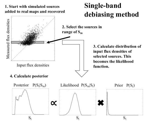
In contrast to previous approaches, which rely on approximate analytic formulations, we numerically estimate the likelihood of by adding simulated sources to the real maps, recovering the sources, and comparing the input and recovered flux densities. We then sample the simulation along slices of fixed by calculating the density distribution of the simulated sources as a function of , at fixed . The resulting function is the likelihood.444Note that the likelihood of the is derived from the conditional distribution of given . Therefore the likelihood is not a distribution of , but rather a function of , which through Bayes’ Theorem allows us to derive the distribution of . Once simulated, the likelihood function can then be multiplied by any number of prior distributions, which depend on assumptions about the underlying source population.
In practice, for a given measured flux density, we identify sources recovered from the simulations that have a similar measured flux density within some tolerance. We identify the input flux densities of these sources, and we estimate the number density of these recovered simulated sources as a function of the input flux density using a kernel density estimator. Note that the likelihood is typically understood as a distribution of measured values, but here we calculate it as a function of intrinsic values, at fixed measured flux density. This lends itself more directly to our goal of the determination of the posterior as a function of the intrinsic flux density. We then multiply this likelihood function by the prior (Equation 2) to calculate the posterior probability distribution, properly normalized, of intrinsic flux density of the brightest source given a measured flux density (Equation 1). The median and 68% confidence interval of this posterior probability distribution are reported as the debiased flux densities. Figure 1 provides a pictorial summary of these methods described for debiasing flux densities in a single band.
2.1 Two-Band Debiasing
In principle, the single-band approach is straightforward to extend to two bands. In this case the posterior is
| (3) |
where subscripts now differentiate between bands as well as intrinsic and measured specifications. The function is a simulated two-band likelihood, and is an analytic prior. This prior can be rewritten as . Here is the single-band prior (Equation 2). The two flux densities are related by a spectral index such that
| (4) |
where and refer to the secondary and primary band frequencies, respectively. There is some distribution for , which allows one to approximate the conditional probability .
An alternative to this formulation, given in C10, re-parameterizes the model in Equation 3 in terms of and . In this case the prior can be rewritten as . Here again is given by Equation 2. The conditional probability is the normalized sum of spectral index distributions for different source types (e.g., AGN and DSFGs in the ACT data), weighted by the number of expected sources of each type, as established by count models for . The resulting posterior can be marginalized to give the single parameter posterior probability for , and, after a transformation of variables, .
In practice, producing simulations comprehensive enough for computing the full two-band likelihood in Equation 3 can be a challenge. This is the case with the ACT data where the required flux densities spanned two orders of magnitude ( mJy) with a broad range of spectral indices. In Gralla et al. (submitted) we implement a simplified version that captures the important aspects of debiasing while proving more tractable computationally.
The approach can be described as follows:
| (5) |
In the second line we make the approximation that the likelihood function of the two bands can be decomposed into independent likelihoods, and . In the third line we have combined the primary-band likelihood with the primary-band prior to produce the primary-band posterior distribution (Equation 1). In the final line, we collapse the product of the posterior and conditional distribution into a joint conditional prior on and . The secondary-band likelihood can be taken as a Gaussian approximation given the raw flux density and error or can be simulated in its own right. Because the source selection is carried out in the primary band, simulating this band is most important to capture selection effects in the likelihood. Conversely, secondary band simulations are less useful unless the secondary band also plays a significant role in source selection.
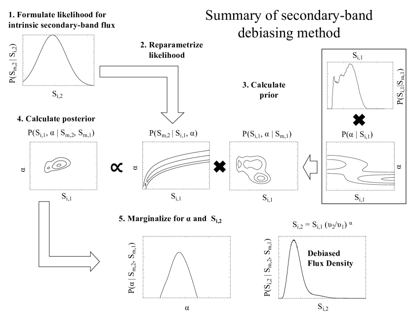
In practice, we calculate this method numerically on one or two-dimensional grids. For instance, to calculate the marginalized probability distribution for starting from Equation 5, each th pixel location in a two-dimensional grid of () is evaluated for its corresponding secondary band flux density according to Equation 4. The one-dimensional probability density array for is computed as
| (6) |
where the sum is performed over the pixels that satisfy . The debiased secondary band flux density can then be calculated from the median (and the uncertainties from the 68% confidence intervals) of this posterior distribution evaluated for all bins, . Figure 2 provides a pictorial summary of these debiasing methods for the flux density of secondary bands.
These methods can be generalized to samples selected by combining multiple bands, as in the case of multi-frequency matched filters. They can also be applied to samples selected from different electromagnetic regimes altogether (such as through the relation between far-infrared and radio). The main requirements are that there is some prior information about the selection that is included (such as the source counts), and that the selection be simulated along with the determination of the flux densities in all bands of interest.
3 Implementation
In this Section, we demonstrate these methods for the debiasing of millimeter sources using simulated sources added to data from the Atacama Cosmology Telescope.
3.1 Constructing the simulated source catalogs
We simulate observations in the 218 GHz ACT band. Because we are interested in the intrinsic flux densities for a population of dusty galaxies, we modeled our simulated source population to be like that expected for dusty galaxies. For each of eighteen trials, we generate 1,000 sources at random positions throughout the maps. Flux densities are randomly assigned according to a Gaussian distribution with mean 10 mJy and standard deviation 5 mJy. This was chosen to provide adequate statistics near the sensitivity limit of the survey, where debiasing is expected to be more important. Because the number of simulated sources drops off at the high end, we supplemented these simulations with 9 trials of simulations populated uniformly in flux density in the range mJy. Because the input flux density distribution was not a uniform random distribution, we normalize the likelihood function that we calculate from these simulations by the distribution of input flux densities.
The 218 GHz flux densities are then scaled by randomly distributed spectral indices to assign flux densities to these sources in the 148 band. The input spectral index distribution is normally distributed as , as based on the sample mean and standard deviation measured from the raw flux densities of the dusty galaxies of a preliminary version of the ACT equatorial catalog (Gralla et al. submitted).
The simulated source template is then added to the map data, which include instrumental and atmospheric noise as well as signal from the cosmic microwave background, Galactic dust, and other compact sources such as AGN and dusty galaxies. Because we use a matched filter in our source recovery (see for example, Marriage et al. 2011), we apply the same filter to both the source template and the data before combining them. We then run the source selection method on the simulated data set and measure the recovered flux densities. Figure 3 shows the input and recovered flux densities for the simulated source sample. Note that the distribution of measured flux densities tends to peak below the input flux densities. This occurs because the input flux density distribution peaks at low (10 mJy) flux densities, so many more faint sources are input to the simulations. As discussed above, we remove this effect by normalizing the calculated likelihood function with the inverse of the input flux density distribution. We verified that the resulting median of the likelihood function agrees with the measured flux density across the full range of flux densities observed.

3.2 An example source
For illustration, we walk through the debiasing of an example source drawn from the simulated sample of dusty galaxies described in Section 3.1. The measured and flux densities are 4 and 17 mJy, respectively. Typically, the primary band is the band for which the S/N is highest. For this example, the primary band is 218 GHz, where the S/N would be about 6.
3.2.1 Single or primary-band debiasing
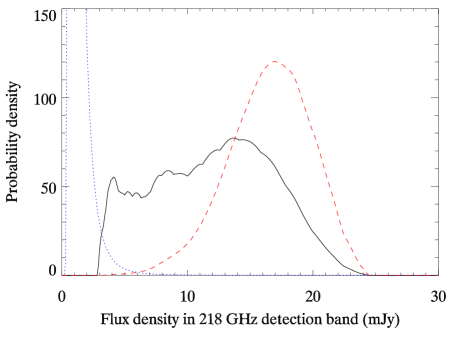
To debias the flux density of the primary band (218 GHz for this example), we must calculate the likelihood function . We select sources from our simulations with a measured value of similar to the value that we are debiasing. The default tolerance for 218 GHz selected sources is 1.0 mJy, so all simulated sources with measured between 16 and 18 mJy are included for this example. See Figure 3 for illustration. We apply a kernel density estimator to the distribution of of these simulated sources. The resulting function of is the likelihood, shown in Figure 4.555For this figure, we used a larger tolerance (1.5 mJy) to increase the statistics in order to better represent the underlying of the distribution. The quoted medians and uncertainty ranges are not affected by this choice.
We calculate the prior probability for according to Equation 2. For the 218 GHz source counts, we construct a model from the addition of a model for AGN source counts from Tucci et al. (2011) (the C2Ex model) and a model for dusty galaxies from Béthermin et al. (2011). The size of the resolution element , or the square of the full width at half maximum of the beam, for ACT is steradians at 148 GHz and steradians at 218 GHz (Hasselfield et al. 2013).
Finally, the posterior probability distribution for is computed from the likelihood function and the prior (Equation 1). The posterior, the likelihood, and the prior for this example source are shown in Figure 4. The debiased flux density that we report at 218 GHz is the median of the posterior distribution, which for this example is 13.2 mJy. The uncertainty is taken to be the confidence interval, which for this example source is mJy.
3.2.2 Secondary band debiasing
After thus debiasing the primary band flux density (218 GHz in this example), we then proceed to debias the secondary bands. We model the likelihood as a Gaussian with mean equal to the measured value and standard deviation equal to the uncertainty on the measurement. We then map this likelihood function to the plane. In practice, for each pixel in a grid, we assign the value where is re-expressed according to Equation 4 as . Figure 5 shows the likelihood for this example.
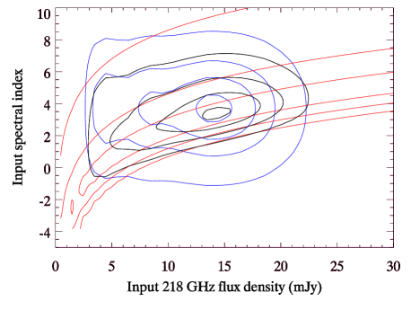
The prior probability distribution factors into two parts. The first part is the posterior shown in Figure 4. The second part of the prior is the conditional probability , which is computed as follows.
For every pixel in the grid of primary band flux densities, we calculate the prior probability density distribution for . For the prior probability of , we use source counts models (Tucci et al. 2011; Béthermin et al. 2011, for AGN and DSFGs, respectively) to calculate the expected ratio of the number of AGN to the number of SFGs as a function of flux density. We model the probability density distribution of the spectral index for each population as Gaussians, for example:
| (7) |
where for subpopulation ( for AGN and for DSFGs) and are the mean and standard deviation in for that subpopulation, respectively. The mean and standard deviation of each Gaussian is determined by calculating the sample median and standard deviation of the distributions for the sources in our catalog (from the region of the map with less noise, and using their measured flux densities prior to debiasing), with the dividing line between AGN and DSFGs defined as . In order to make the prior on somewhat less constraining of the resulting flux densities, we choose the standard deviation to be greater than that of the measured sample standard deviation. This widens the prior on , which when normalized then has less constraining power on the measurement-based likelihood function. For AGN, the prior we use has median and the standard deviation is (the sample standard deviation is 0.9). For the DSFGs, the median and the standard deviation is (the sample standard deviation is 1.6).666We tested our sensitivity to the width of the prior on by also calculating the debiasing using the narrower sample standard deviations instead and comparing the results. We found that the majority of the sample is not affected, but that in particular, outliers classified as DSFGs that have weaker 148 GHz detections are more debiased when the prior distribution is narrower. This behavior is expected: intuitively, the unchanged prior on the mean implies that most of the sample should be unchanged, but for sources that deviate from the mean behavior, a tighter prior on brings more statistical weight from the primary band to bear on the debiasing calculated for the secondary band. We scale each of these distributions by the fraction of sources expected based on the counts models, and add the distributions together to get a distribution for as a function of flux density:
| (8) |
where and are the fractions of AGN and DSFGs, respectively, as determined by the source counts models, and and are calculated according to Equation 7. For each pixel, we multiply the conditional probability for by the posterior probability for :
| (9) |
The resulting prior is shown in blue in Figure 5.
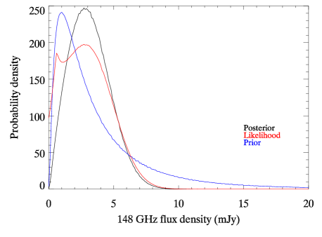
To calculate the posterior distribution for the intrinsic 148 GHz flux density, we multiply each pixel of the prior (which is a function of and ) by each pixel of the likelihood function (which similarly is calculated as a function of and ). Figure 6 shows the posterior distribution that results. For each of these pixels, we calculate the 148 GHz flux density from the and . We sum the probability density of all the , pixels that correspond to a given 148 GHz flux density (Equation 6). This procedure produces the posterior probability density function for the 148 GHz flux density, shown in Figure 6. The median of the posterior distribution is reported as the debiased flux density at 148 GHz. For this example source, the debiased 148 GHz flux density is 3.1 mJy. The confidence interval of the posterior distribution for this example source ranges from 1.7 to 4.8 mJy.
3.3 Details
The implementation of the multi-band debiasing methods requires a number of choices, which are described here in more detail. These choices include selecting an adequate number of simulated sources to derive the likelihood function, selecting a radius for matching the recovered simulated sources with input sources, selecting the tolerance in flux density for selecting simulated sources with measured flux density close to that of the source being debiased, and selecting the kernel size of the kernel density estimator used to calculate the likelihood function.
To test whether the simulated source sample is sufficiently large, we ran the debiasing on an example source (with 148 and 218 flux densities of 25 mJy) using only half of the simulated sources. The debiased flux densities agreed with those calculated from the entire simulated source sample, indicating that the number of sources in our simulations is sufficient for sampling the likelihood function.
To compute the flux density likelihood , we associate sources detected from the maps with input simulated sources. In so doing we must use an association radius. As discussed in Gralla et al. (submitted), the ACT positional uncertainty of sources with above 5 is typically less than 0.005 degrees. We adopt 0.007 degrees, or , as our match radius. One of the simulated sources was randomly positioned close (within the 0.002 degree tolerance) to a real, bright source in the catalog, and it was excluded from the sample. We exclude cases in which two sources are measured to match an input source position.
Our debiasing method requires that we identify sources from the simulations with flux densities similar to the catalog source that we are debiasing. The default tolerance we use for 218 GHz selected sources is mJy. For 148 GHz selected sources and sources selected through our DSFG-optimized multi-frequency matched filter (MMF), we use a tolerance of mJy. For more details on 148 GHz and MMF selection, see the catalog paper (Gralla et al. submitted).
At the low flux density end, the completeness affects the source recovery, such that the number of sources drops off very quickly toward low flux densities. Because of the steepness of this completeness cut off, we must use a narrower tolerance when debiasing sources to avoid biasing the debiased flux density high, as lower flux density sources have not been detected. Thus for sources with flux densities in the region of steeply falling completeness (below 25 mJy for 148 GHz selected sources), we reduce the tolerance to mJy. To test whether the choice of tolerance has an significant effect, if we adopt mJy as the tolerance, a value substantially less than the typical noise level ( mJy), the debiased flux densities do not change significantly compared to the mJy tolerance. We note that this result is not surprising: the mJy tolerance designates the limits of a uniform distribution, the effective standard error of which is mJy. Added in quadrature with the error on the likelihood, this choice only broadens the recovered posterior by 2%.
The kernel density estimator we use to calculate the likelihood from the distribution of simulated sources requires specifying a scale for the kernel size, which can affect the results. Kernels that are too large would artificially smooth the likelihood function, inflating the tails of the distribution. Kernels that are too small would introduce noise into the likelihood function. After investigating a range of kernel scales, we set the kernel scale to 1.0 mJy.
In addition to the choices discussed above, care must be taken when using the simulated source catalogs, particularly regarding spurious matches. For example, consider faint simulated sources that are spuriously matched with brighter real (or simulated) sources. When calculating the likelihood function of a source with measured flux densities like the brighter source, these spurious sources would contribute at low intrinsic flux densities. When this likelihood function is multiplied by the steep prior, this effect is amplified. Such sources must be vetoed from the simulations as they are not, by construction, the brightest source associated with a detection, which is what the likelihood is built to describe. For additional details of the application of these methods to the ACT data, such as the selection of the match radius and the handling of spurious matches, see Gralla et al. (submitted).
3.4 Method applied to a population
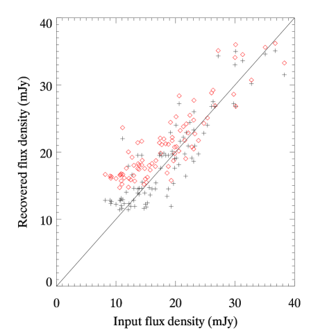
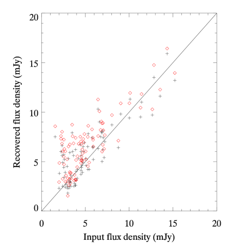
Finally, we used a second set of simulations to verify that the debiasing methods do indeed bring the flux densities into agreement with intrinsic flux densities. For this test, we populated the maps with sources with flux densities drawn according to the source counts model for the dusty source population, populating a range between 7 and 40 mJy. The spectral index of each source was drawn from a Gaussian distribution with mean 3.4 and width 1.0, which is motivated by the measured spectral index distribution for dusty galaxies in the ACT catalog. After performing the full source finding and flux density debiasing on this sample, we compare the input and debiased flux densities, shown in Figure 7. As seen in this figure, the debiased flux densities improve upon the measured flux densities in recovering the input flux densities for this simulated dusty source sample. The median of the ratio of the input flux density to the debiased flux density is 0.98 for 218 GHz and 0.95 for 148 GHz. For comparison, the median of the ratio of the input flux density to the measured flux density is 0.88 for 218 GHz and 0.82 for 148 GHz.
4 Conclusions
We have presented a new Bayesian method for debiasing source flux density estimates. The method combines an analytic prior with simulations for computing the likelihood of the intrinsic flux density. The simulations capture details of nontrivial source selection while the analytic prior provides a fast and flexible way to correct for flux bias arising from steeply falling counts. In the companion catalog paper (Gralla et al. submitted), we explore this method applied to DSFGs selected with a multifrequency matched filter with the additional complication of population culling to reduce contamination from Galactic sources. In this paper we have derived the method, provided a symbolic guide to implementation, and illustrated the steps applied to an example source. We have also shown how the method debiases the flux densities of a population of DSFGs with steeply falling number counts.
Acknowledgements
We thank Eric Switzer, Tom Crawford, and Bruce Partridge for useful discussions and comments. This work was supported by the U.S. National Science Foundation through awards AST-0408698 and AST-0965625 for the ACT project, as well as awards PHY-0855887 and PHY-1214379. Funding was also provided by Princeton University, the University of Pennsylvania, and a Canada Foundation for Innovation (CFI) award to UBC. ACT operates in the Parque Astronómico Atacama in northern Chile under the auspices of the Comisión Nacional de Investigación Científica y Tecnológica de Chile (CONICYT). Computations were performed on the GPC supercomputer at the SciNet HPC Consortium. SciNet is funded by the CFI under the auspices of Compute Canada, the Government of Ontario, the Ontario Research Fund – Research Excellence; and the University of Toronto. M.G. and T.M. acknowledge support from Johns Hopkins University.
References
- Austermann et al. (2009) Austermann, J. E. et al. 2009, MNRAS, 393, 1573
- Austermann et al. (2010) —. 2010, MNRAS, 401, 160
- Béthermin et al. (2011) Béthermin, M., Dole, H., Lagache, G., Le Borgne, D., & Penin, A. 2011, A&A, 529, A4
- Coppin et al. (2006) Coppin, K. et al. 2006, MNRAS, 372, 1621
- Coppin et al. (2005) Coppin, K., Halpern, M., Scott, D., Borys, C., & Chapman, S. 2005, MNRAS, 357, 1022
- Crawford et al. (2010) Crawford, T. M., Switzer, E. R., Holzapfel, W. L., Reichardt, C. L., Marrone, D. P., & Vieira, J. D. 2010, ApJ, 718, 513
- Datta et al. (2019) Datta, R. et al. 2019, MNRAS, 486, 5239
- Eddington (1913) Eddington, A. S. 1913, Monthly Notices of the Royal Astronomical Society, 73, 359
- Gralla et al. (submitted) Gralla, M. B. et al. submitted, ApJ
- Hasselfield et al. (2013) Hasselfield, M. et al. 2013, ArXiv e-prints
- Hogg & Turner (1998) Hogg, D. W., & Turner, E. L. 1998, PASP, 110, 727
- Jauncey (1968) Jauncey, D. L. 1968, ApJ, 152, 647
- Marriage et al. (2011) Marriage, T. A. et al. 2011, ApJ, 731, 100
- Marsden et al. (2014) Marsden, D. et al. 2014, MNRAS, 439, 1556
- Mocanu et al. (2013) Mocanu, L. M. et al. 2013, ApJ, 779, 61
- Murdoch et al. (1973) Murdoch, H. S., Crawford, D. F., & Jauncey, D. L. 1973, ApJ, 183, 1
- Oliver et al. (2010) Oliver, S. J. et al. 2010, A&A, 518, L21
- Schmitt & Maccacaro (1986) Schmitt, J. H. M. M., & Maccacaro, T. 1986, ApJ, 310, 334
- Swetz et al. (2011) Swetz, D. S. et al. 2011, ApJS, 194, 41
- Tucci et al. (2011) Tucci, M., Toffolatti, L., de Zotti, G., & Martínez-González, E. 2011, A&A, 533, A57
- Valiante et al. (2016) Valiante, E. et al. 2016, MNRAS, 462, 3146
- Vieira et al. (2010) Vieira, J. D. et al. 2010, ApJ, 719, 763