Hessian transport Gradient flows

Wuchen Li Department of Mathematics, University of California, Los Angeles. wcli@math.ucla.edu  and  Lexing Ying Department of Mathematics, Stanford University and Facebook AI Research lexing@stanford.edu
Abstract.

We derive new gradient flows of divergence functions in the probability space embedded with a class of Riemannian metrics. The Riemannian metric tensor is built from the transported Hessian operator of an entropy function. The new gradient flow is a generalized Fokker-Planck equation and is associated with a stochastic differential equation that depends on the reference measure. Several examples of Hessian transport gradient flows and the associated stochastic differential equations are presented, including the ones for the reverse Kullback–Leibler divergence, α𝛼\alpha-divergence, Hellinger distance, Pearson divergence, and Jenson–Shannon divergence.

Key words and phrases:
Optimal transport; Information/Hessian geometry; Hessian transport; Hessian transport stochastic differential equations; Generalized de Bruijn identity.

1. Introduction

The de Bruijn identity plays crucial roles in information theory, probability, statistics, geometry, and machine learning [10, 11, 12, 26, 30, 34]. It states that the dissipation of the relative entropy, also known as the Kullback–Leibler (KL) divergence function, along the heat flow is equal to the relative Fisher information functional. This identity is important for many applications in Bayesian statistics and Markov chain Monte Carlo methods.

It turns out that there are two geometric structures in the probability space related to the de Bruijn identity. One is Wasserstein geometry (WG) [14, 32], which refers to the heat flows or Gaussian kernels. In [13, 28], it shows that the gradient flow of the negative Boltzmann Shannon entropy in WG is the heat equation. The de Bruijn identity can be understood as the rate of entropy dissipation within WG. The other one is information geometry (IG) [1, 5], which relates to the differential structures of the entropy. IG studies various families of Hessian geometry of entropy and divergence functions. Here, the Boltzmann-Shannon entropy, the Fisher-Rao metric, and the further induced KL divergence function are of particular importance. Besides these classical cases, one also studies generalized entropy and divergence functions, such as Tsallis entropy and Tsallis divergence [2, 31].

A natural question arises: What are natural families of geometries in the probability space that connect entropy/divergence functions, heat flows, and the de Bruijn identity?
Refer to caption
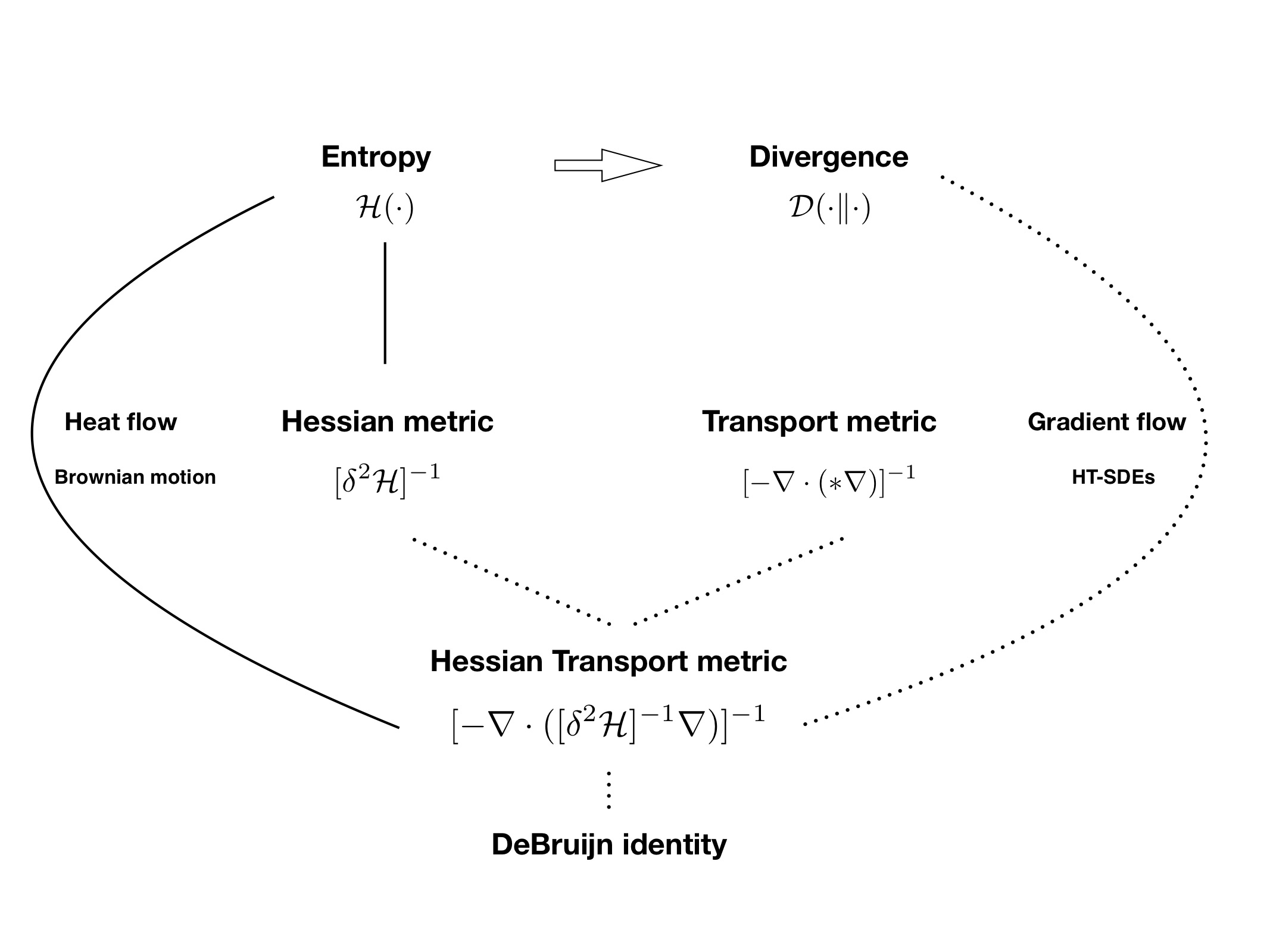
Figure 1. Derivation Diagram of the Hessian transport metric. The real lines are results in classical WG or IG communities. The dot lines are results derived in this paper.

In this paper, we positively answer this question by introducing a family of Riemannian metrics in the probability space. Consider a compact space ΩΩ\Omega and a positive smooth probability space 𝒫(Ω)𝒫Ω\mathcal{P}(\Omega). For a strictly convex entropy function :𝒫(Ω):𝒫Ω\mathcal{H}\colon\mathcal{P}(\Omega)\rightarrow\mathbb{R}, we introduce a new Riemannian metric tensor Gsubscript𝐺G_{\mathcal{H}} in the probability space

G(ρ)1=[([δ2(ρ)]1)],subscript𝐺superscript𝜌1delimited-[]superscriptdelimited-[]superscript𝛿2𝜌1G_{\mathcal{H}}(\rho)^{-1}=[-\nabla\cdot([\delta^{2}\mathcal{H}(\rho)]^{-1}\nabla)],

where ρ𝒫(Ω)𝜌𝒫Ω\rho\in\mathcal{P}(\Omega) is a probability density function, δ2(ρ)superscript𝛿2𝜌\delta^{2}\mathcal{H}(\rho) is the L2superscript𝐿2L^{2} Hessian operator of the entropy function, and finally \nabla and \nabla\cdot are gradient and divergence operators on ΩΩ\Omega, respectively. We refer to Definition 1 for the formal definition. Notice that the proposed metric involves both the Hessian geometry of \mathcal{H} and the transport metric (gradient and divergence operator on sample space). For this reason, it is called the Hessian transport metric (HT-metric) (see Figure 1 for a schematic diagram).

As a simple but motivating example, the heat equation is the gradient flow of the entropy function \mathcal{H} under the HT-metric Gsubscript𝐺G_{\mathcal{H}} induced by \mathcal{H} itself:

tρ=G(ρ)1δ(ρ)=(([δ2(ρ)]1δ(ρ)))=([δ2(ρ)]1[δ2(ρ)]ρ)=(ρ)=Δρ.subscript𝑡𝜌subscript𝐺superscript𝜌1𝛿𝜌superscriptdelimited-[]superscript𝛿2𝜌1𝛿𝜌superscriptdelimited-[]superscript𝛿2𝜌1delimited-[]superscript𝛿2𝜌𝜌𝜌Δ𝜌\begin{split}\partial_{t}\rho=&-G_{\mathcal{H}}(\rho)^{-1}\delta\mathcal{H}(\rho)\\ =&-\Big{(}-\nabla\cdot([\delta^{2}\mathcal{H}(\rho)]^{-1}\nabla\delta\mathcal{H}(\rho))\Big{)}\\ =&\nabla\cdot([\delta^{2}\mathcal{H}(\rho)]^{-1}[\delta^{2}\mathcal{H}(\rho)]\nabla\rho)\\ =&\nabla\cdot(\nabla\rho)=\Delta\rho.\end{split}

In a more general setting, we consider a family of entropy functions of form f(ρ)=Ωf(ρ)𝑑xsubscript𝑓𝜌subscriptΩ𝑓𝜌differential-d𝑥\mathcal{H}_{f}(\rho)=\int_{\Omega}f(\rho)dx, where f()𝑓f(\cdot) is convex, f(1)=0𝑓10f(1)=0 and f′′superscript𝑓′′f^{\prime\prime} is homogeneous of degree (γ)𝛾(-\gamma). For a fixed reference measure μ𝜇\mu, there is an associated divergence function 𝒟f(ρμ)=Ωf(ρμ)μ𝑑xsubscript𝒟𝑓conditional𝜌𝜇subscriptΩ𝑓𝜌𝜇𝜇differential-d𝑥\mathcal{D}_{f}(\rho\|\mu)=\int_{\Omega}f(\frac{\rho}{\mu})\mu dx for each fsubscript𝑓\mathcal{H}_{f}. By considering the gradient flow of 𝒟f(ρμ)subscript𝒟𝑓conditional𝜌𝜇\mathcal{D}_{f}(\rho\|\mu) in (𝒫(Ω),Gf)𝒫Ωsubscript𝐺subscript𝑓(\mathcal{P}(\Omega),G_{\mathcal{H}_{f}}), we derive a generalized Fokker-Planck equation

tρ(t,x)=(μ(x)γ(ρ(t,x)μ(x))),subscript𝑡𝜌𝑡𝑥𝜇superscript𝑥𝛾𝜌𝑡𝑥𝜇𝑥\partial_{t}\rho(t,x)=\nabla\cdot\left(\mu(x)^{\gamma}\nabla\left(\frac{\rho(t,x)}{\mu(x)}\right)\right),

along with a stochastic differential equation for independent particle dynamics

dXt=γμ(Xt)γ2μ(Xt)dt+2μ(Xt)γ1dBt,𝑑subscript𝑋𝑡𝛾𝜇superscriptsubscript𝑋𝑡𝛾2𝜇subscript𝑋𝑡𝑑𝑡2𝜇superscriptsubscript𝑋𝑡𝛾1𝑑subscript𝐵𝑡dX_{t}=\gamma\mu(X_{t})^{\gamma-2}\nabla\mu(X_{t})dt+\sqrt{2\mu(X_{t})^{\gamma-1}}dB_{t},

where Btsubscript𝐵𝑡B_{t} is the standard Brownian motion. Such a SDE is called a Hessian transport stochastic differential equation (HT-SDE).

It is worth mentioning that two special cases of HT-metrics and their induced HT-SDEs are particularly relevant. When γ=1𝛾1\gamma=1, (ρ)𝜌\mathcal{H}(\rho) is the Boltzmann-Shannon entropy, the HT-metric is the usual Wasserstein-2 metric and the HT-SDE is the classical Langevin dynamics. When γ=0𝛾0\gamma=0, (ρ)𝜌\mathcal{H}(\rho) is the Pearson divergence, the HT-metric is the H1superscript𝐻1H^{-1} metric and the associated HT-SDE is a diffusion process with zero drift. We refer to Table 1 for a summary of the results.

Currently, there are several efforts in combining both Wasserstein metric and information/Hessian metric [3, 6, 7, 8, 9, 19, 24, 33] from various perspectives. Within the Gaussian families, several extensions are studied in [25]. Another example from the machine learning community is the Stein variational gradient descent method [21, 22, 23]. Here we introduce a new geometry structure, which keeps heat flows as gradient flows of general entropy functions. We emphasize the interaction relations between Hessian of entropy and transport metric. Our approach is a natural extension to both IG and WG. It can also be viewed as a generalization for the field of Wasserstein information geometry [15, 17, 18].

The rest of this paper is organized as follows. In Section 2, we define the Hessian transport metric and show that the heat flow can be interpreted as the gradient flow of several energy functions under appropriate HT-metrics. We then move on to derive, for general divergence functions, the HT-metric gradient flows and the associated HT-SDEs. In Section 3, we introduce the Hessian transport distance (HT-distance) and derive the corresponding HT-geodesic equation. Several numerical examples are given in Section 4.

Divergence Inverse HT-Metric Relative Fisher divergence HT-Gradient flow HT-SDE HT-geodesics
ΩρlogρμdxsubscriptΩ𝜌𝜌𝜇𝑑𝑥\int_{\Omega}\rho\log{\frac{\rho}{\mu}}dx (ρ)𝜌-\nabla\cdot(\rho\nabla) Ωlogρμ2ρ𝑑xsubscriptΩsuperscriptnorm𝜌𝜇2𝜌differential-d𝑥\int_{\Omega}\left\|\nabla\log\frac{\rho}{\mu}\right\|^{2}\rho dx tρ=(ρlogμ)+Δρsubscript𝑡𝜌𝜌𝜇Δ𝜌\partial_{t}\rho=\nabla\cdot(\rho\nabla\log\mu)+\Delta\rho dXt=logμdt+2Bt𝑑subscript𝑋𝑡𝜇𝑑𝑡2subscript𝐵𝑡dX_{t}=\nabla\log\mu dt+\sqrt{2}B_{t} {tρ+(ρΦ)=0tΦ+12(Φ,Φ)=0casesotherwisesubscript𝑡𝜌𝜌Φ0otherwisesubscript𝑡Φ12ΦΦ0\begin{cases}&\partial_{t}\rho+\nabla\cdot(\rho\nabla\Phi)=0\\ &\partial_{t}\Phi+\frac{1}{2}(\nabla\Phi,\nabla\Phi)=0\end{cases}
ΩμlogμρdxsubscriptΩ𝜇𝜇𝜌𝑑𝑥-\int_{\Omega}\mu\log{\frac{\mu}{\rho}}dx (ρ2)superscript𝜌2-\nabla\cdot(\rho^{2}\nabla) Ω(ρμ)12ρ2dx\int_{\Omega}\left\|\nabla\Big{(}\frac{\rho}{\mu}\Big{)}^{-1}\right\|^{2}\rho^{2}dx tρ=(μ2(ρμ))subscript𝑡𝜌superscript𝜇2𝜌𝜇\partial_{t}\rho=\nabla\cdot\left(\mu^{2}\nabla\left(\frac{\rho}{\mu}\right)\right) dXt=2μdt+2μdBt𝑑subscript𝑋𝑡2𝜇𝑑𝑡2𝜇𝑑subscript𝐵𝑡dX_{t}=2\nabla\mu dt+\sqrt{2\mu}dB_{t} {tρ+(ρ2Φ)=0tΦ+(Φ,Φ)ρ=0casesotherwisesubscript𝑡𝜌superscript𝜌2Φ0otherwisesubscript𝑡ΦΦΦ𝜌0\begin{cases}&\partial_{t}\rho+\nabla\cdot(\rho^{2}\nabla\Phi)=0\\ &\partial_{t}\Phi+(\nabla\Phi,\nabla\Phi)\rho=0\end{cases}
Ω41α2(1(ρμ)1+α2)μ𝑑xsubscriptΩ41superscript𝛼21superscript𝜌𝜇1𝛼2𝜇differential-d𝑥\int_{\Omega}\frac{4}{1-\alpha^{2}}(1-(\frac{\rho}{\mu})^{\frac{1+\alpha}{2}})\mu dx (ρ3α2)superscript𝜌3𝛼2-\nabla\cdot(\rho^{\frac{3-\alpha}{2}}\nabla) (2α1)2Ω(ρμ)α122ρ3α2dx(\frac{2}{\alpha-1})^{2}\int_{\Omega}\left\|\nabla\Big{(}\frac{\rho}{\mu}\Big{)}^{\frac{\alpha-1}{2}}\right\|^{2}\rho^{\frac{3-\alpha}{2}}dx tρ=(μ(3α)/2(ρμ))subscript𝑡𝜌superscript𝜇3𝛼2𝜌𝜇\partial_{t}\rho=\nabla\cdot\left(\mu^{(3-\alpha)/2}\nabla\left(\frac{\rho}{\mu}\right)\right) dXt=3α2μ1α2μdt+2μ1α2dBt𝑑subscript𝑋𝑡3𝛼2superscript𝜇1𝛼2𝜇𝑑𝑡2superscript𝜇1𝛼2𝑑subscript𝐵𝑡dX_{t}=\frac{3-\alpha}{2}\mu^{\frac{-1-\alpha}{2}}\nabla\mu dt+\sqrt{2\mu^{\frac{1-\alpha}{2}}}dB_{t} {tρ+(ρ3α2Φ)=0tΦ+3α2(Φ,Φ)ρ1α2=0casesotherwisesubscript𝑡𝜌superscript𝜌3𝛼2Φ0otherwisesubscript𝑡Φ3𝛼2ΦΦsuperscript𝜌1𝛼20\begin{cases}&\partial_{t}\rho+\nabla\cdot(\rho^{\frac{3-\alpha}{2}}\nabla\Phi)=0\\ &\partial_{t}\Phi+\frac{3-\alpha}{2}(\nabla\Phi,\nabla\Phi)\rho^{\frac{1-\alpha}{2}}=0\end{cases}
Ω(ρμ)2𝑑xsubscriptΩsuperscript𝜌𝜇2differential-d𝑥\int_{\Omega}(\sqrt{\rho}-\sqrt{\mu})^{2}dx (ρ32)superscript𝜌32-\nabla\cdot(\rho^{\frac{3}{2}}\nabla) 4Ω(ρμ)122ρ32dx4\int_{\Omega}\left\|\nabla\Big{(}\frac{\rho}{\mu}\Big{)}^{-\frac{1}{2}}\right\|^{2}\rho^{\frac{3}{2}}dx tρ=(μ3/2(ρμ))subscript𝑡𝜌superscript𝜇32𝜌𝜇\partial_{t}\rho=\nabla\cdot\left(\mu^{3/2}\nabla\left(\frac{\rho}{\mu}\right)\right) dXt=32μ12μdt+2μ12dBt𝑑subscript𝑋𝑡32superscript𝜇12𝜇𝑑𝑡2superscript𝜇12𝑑subscript𝐵𝑡dX_{t}=\frac{3}{2}\mu^{-\frac{1}{2}}\nabla\mu dt+\sqrt{2\mu^{\frac{1}{2}}}dB_{t} {tρ+(ρ32Φ)=0tΦ+32(Φ,Φ)ρ12=0casesotherwisesubscript𝑡𝜌superscript𝜌32Φ0otherwisesubscript𝑡Φ32ΦΦsuperscript𝜌120\begin{cases}&\partial_{t}\rho+\nabla\cdot(\rho^{\frac{3}{2}}\nabla\Phi)=0\\ &\partial_{t}\Phi+\frac{3}{2}(\nabla\Phi,\nabla\Phi)\rho^{\frac{1}{2}}=0\end{cases}
Ω(ρμ1)2μ𝑑xsubscriptΩsuperscript𝜌𝜇12𝜇differential-d𝑥\int_{\Omega}(\frac{\rho}{\mu}-1)^{2}\mu dx ()-\nabla\cdot(\nabla) Ω(ρμ)2𝑑xsubscriptΩsuperscriptnorm𝜌𝜇2differential-d𝑥\int_{\Omega}\left\|\nabla\Big{(}\frac{\rho}{\mu}\Big{)}\right\|^{2}dx tρ=((ρμ))subscript𝑡𝜌𝜌𝜇\partial_{t}\rho=\nabla\cdot(\nabla(\frac{\rho}{\mu})) dXt=2μ1dBt𝑑subscript𝑋𝑡2superscript𝜇1𝑑subscript𝐵𝑡dX_{t}=\sqrt{2\mu^{-1}}dB_{t} {tρ+ΔΦ=0tΦ=0casesotherwisesubscript𝑡𝜌ΔΦ0otherwisesubscript𝑡Φ0\begin{cases}&\partial_{t}\rho+\Delta\Phi=0\\ &\partial_{t}\Phi=0\end{cases}
Ωρlogρ12(ρ+μ)+μlogμ12(ρ+μ)dxsubscriptΩ𝜌𝜌12𝜌𝜇𝜇𝜇12𝜌𝜇𝑑𝑥\int_{\Omega}\rho\log\frac{\rho}{\frac{1}{2}(\rho+\mu)}+\mu\log\frac{\mu}{\frac{1}{2}(\rho+\mu)}dx (ρ(1+ρ))𝜌1𝜌-\nabla\cdot(\rho(1+\rho)\nabla) Ωlog(2ρρ+μ)2ρ(1+ρ)𝑑xsubscriptΩsuperscriptnorm2𝜌𝜌𝜇2𝜌1𝜌differential-d𝑥\int_{\Omega}\left\|\nabla\log(\frac{2\rho}{\rho+\mu})\right\|^{2}\rho(1+\rho)dx tρ=((1+ρ)μ2ρ+μ(ρμ))subscript𝑡𝜌1𝜌superscript𝜇2𝜌𝜇𝜌𝜇\partial_{t}\rho=\nabla\cdot\Big{(}\frac{(1+\rho)\mu^{2}}{\rho+\mu}\nabla(\frac{\rho}{\mu})\Big{)} - {tρ+(ρ(1+ρ)Φ)=0tΦ+12(Φ,Φ)(2ρ+1)=0casesotherwisesubscript𝑡𝜌𝜌1𝜌Φ0otherwisesubscript𝑡Φ12ΦΦ2𝜌10\begin{cases}&\partial_{t}\rho+\nabla\cdot(\rho(1+\rho)\nabla\Phi)=0\\ &\partial_{t}\Phi+\frac{1}{2}(\nabla\Phi,\nabla\Phi)(2\rho+1)=0\end{cases}
Table 1. In this table, we present the Hessian transport for KL divergence, reverse KL divergence, α𝛼\alpha-divergence, Hellinger distance, Pearson divergence, and Jensen-Shannon divergence. In the case α=1𝛼1\alpha=1, the HT-metric recovers the Wasserstein-2 metric from the classical optimal transport theory. In the case of α=3𝛼3\alpha=3, the HT-metric recovers the H1superscript𝐻1H^{-1} metric.

2. Hessian transport Gradient flows

In this section, we introduce the Hessian transport metrics and derive the gradient flows under these metrics.

2.1. Motivations

Consider a compact space ΩdΩsuperscript𝑑\Omega\subset\mathbb{R}^{d}. Following the usual convention, we denote by \nabla and \nabla\cdot the gradient and divergence operators in ΩΩ\Omega and by δ𝛿\delta, \|\cdot\| the Euclidean norm in dsuperscript𝑑\mathbb{R}^{d}, δ2superscript𝛿2\delta^{2} the first and the second L2superscript𝐿2L^{2} variations. From now on, the boundary conditions on ΩΩ\Omega are given by either Neumann or periodic boundary conditions.

The heat equation

tρ(t,x)=Δρ(t,x),subscript𝑡𝜌𝑡𝑥Δ𝜌𝑡𝑥\partial_{t}\rho(t,x)=\Delta\rho(t,x), (1)

can be written in several equivalent ways as follows

tρ(t,x)=subscript𝑡𝜌𝑡𝑥absent\displaystyle\partial_{t}\rho(t,x)= (ρ(t,x))𝜌𝑡𝑥\displaystyle\nabla\cdot\Big{(}\nabla\rho(t,x)\Big{)}
tρ(t,x)=subscript𝑡𝜌𝑡𝑥absent\displaystyle\partial_{t}\rho(t,x)= (ρ(t,x)logρ(t,x))𝜌𝑡𝑥𝜌𝑡𝑥\displaystyle\nabla\cdot\Big{(}\rho(t,x)\nabla\log\rho(t,x)\Big{)}
tρ(t,x)=subscript𝑡𝜌𝑡𝑥absent\displaystyle\partial_{t}\rho(t,x)= (ρ(t,x)2(1ρ(t,x))),𝜌superscript𝑡𝑥21𝜌𝑡𝑥\displaystyle\nabla\cdot\left(\rho(t,x)^{2}\nabla\left(-\frac{1}{\rho(t,x)}\right)\right),

where the following relation is used

ρ=ρlogρ=ρ2(1ρ).𝜌𝜌𝜌superscript𝜌21𝜌\nabla\rho=\rho\nabla\log\rho=\rho^{2}\nabla\left(-\frac{1}{\rho}\right).

These formulas show that the heat flow has multiple gradient descent flow interpretations. Recall that a general gradient flow takes the form

tρ=G(ρ)1δ(ρ),subscript𝑡𝜌𝐺superscript𝜌1𝛿𝜌\partial_{t}\rho=-G(\rho)^{-1}\delta\mathcal{E}(\rho),

where ()\mathcal{E}(\cdot) is an energy function and the operator G(ρ):C(Ω)C(Ω):𝐺𝜌superscript𝐶Ωsuperscript𝐶ΩG(\rho)\colon C^{\infty}(\Omega)\rightarrow C^{\infty}(\Omega) represents the metric tensor. Under this framework, the heat equation can be interpreted in several ways:

  • (i)

    Dirichlet energy formulation:

    (ρ)=Ωρ(x)2𝑑x,δ(ρ)=Δρ,G(ρ)1=𝕀,formulae-sequence𝜌subscriptΩsuperscriptnorm𝜌𝑥2differential-d𝑥formulae-sequence𝛿𝜌Δ𝜌𝐺superscript𝜌1𝕀\mathcal{E}(\rho)=\int_{\Omega}\|\nabla\rho(x)\|^{2}dx,\quad\delta\mathcal{E}(\rho)=-\Delta\rho,\quad G(\rho)^{-1}=\mathbb{I},

    where 𝕀:C(Ω)C(Ω):𝕀superscript𝐶Ωsuperscript𝐶Ω\mathbb{I}\colon C^{\infty}(\Omega)\rightarrow C^{\infty}(\Omega) is the identity operator. Then

    tρ=G(ρ)1δ(ρ)=(Δρ)=Δρ.subscript𝑡𝜌𝐺superscript𝜌1𝛿𝜌Δ𝜌Δ𝜌\partial_{t}\rho=-G(\rho)^{-1}\delta\mathcal{E}(\rho)=-(-\Delta\rho)=\Delta\rho.
  • (ii)

    Boltzmann-Shannon entropy formulation:

    (ρ)=Ωρ(x)logρ(x)𝑑x,δ(ρ)=logρ+1,G(ρ)1=(ρ).formulae-sequence𝜌subscriptΩ𝜌𝑥𝜌𝑥differential-d𝑥formulae-sequence𝛿𝜌𝜌1𝐺superscript𝜌1𝜌\mathcal{E}(\rho)=\int_{\Omega}\rho(x)\log\rho(x)dx,\quad\delta\mathcal{E}(\rho)=\log\rho+1,\quad G(\rho)^{-1}=-\nabla\cdot(\rho\nabla).
    tρ=G(ρ)1δ(ρ)=((ρlogρ))=Δρ.subscript𝑡𝜌𝐺superscript𝜌1𝛿𝜌𝜌𝜌Δ𝜌\partial_{t}\rho=-G(\rho)^{-1}\delta\mathcal{E}(\rho)=-(-\nabla\cdot(\rho\nabla\log\rho))=\Delta\rho.
  • (iii)

    Cross entropy formulation:111Given μC(Ω)𝜇superscript𝐶Ω\mu\in C^{\infty}(\Omega), the cross entropy is defined as follows (ρ,μ)=Ωμ(x)logρ(x)𝑑x𝜌𝜇subscriptΩ𝜇𝑥𝜌𝑥differential-d𝑥\mathcal{H}(\rho,\mu)=-\int_{\Omega}\mu(x)\log\rho(x)dx Here we let μ(x)=1𝜇𝑥1\mu(x)=1, for all xΩ𝑥Ωx\in\Omega.

    (ρ)=Ωlogρ(x)𝑑x,δ(ρ)=1ρ,G(ρ)1=(ρ2).formulae-sequence𝜌subscriptΩ𝜌𝑥differential-d𝑥formulae-sequence𝛿𝜌1𝜌𝐺superscript𝜌1superscript𝜌2\mathcal{E}(\rho)=-\int_{\Omega}\log\rho(x)dx,\quad\delta\mathcal{E}(\rho)=-\frac{1}{\rho},\quad G(\rho)^{-1}=-\nabla\cdot(\rho^{2}\nabla).
    tρ=G(ρ)1δ(ρ)=((ρ2(1ρ)))=Δρ.subscript𝑡𝜌𝐺superscript𝜌1𝛿𝜌superscript𝜌21𝜌Δ𝜌\partial_{t}\rho=-G(\rho)^{-1}\delta\mathcal{E}(\rho)=-\left(-\nabla\cdot\left(\rho^{2}\nabla\left(-\frac{1}{\rho}\right)\right)\right)=\Delta\rho.

It is clear that the metric G𝐺G and the energy \mathcal{E} need to be compatible in order to give rise the heat equation. In fact, given a strictly convex energy function \mathcal{E} in the probability space, it induces a compatible metric operator

G(ρ)1:=(([δ2(ρ)]1)),assign𝐺superscript𝜌1superscriptdelimited-[]superscript𝛿2𝜌1G(\rho)^{-1}:=\Big{(}-\nabla\cdot([\delta^{2}\mathcal{E}(\rho)]^{-1}\nabla)\Big{)},

which combines both the transport operator (gradient, divergence operator in ΩΩ\Omega) and the L2superscript𝐿2L^{2} Hessian operator of \mathcal{E}. Following this relation, the heat equation can be viewed as the gradient flow of the energy \mathcal{E} under the \mathcal{E}-induced metric operator. Below we include the calculations of the above three cases for the sake of completeness.

  • (i)

    Dirichlet energy formulation:

    (ρ)=Ωρ(x)2𝑑x,δ2(ρ)=Δ,formulae-sequence𝜌subscriptΩsuperscriptnorm𝜌𝑥2differential-d𝑥superscript𝛿2𝜌Δ\mathcal{E}(\rho)=\int_{\Omega}\|\nabla\rho(x)\|^{2}dx,\quad\delta^{2}\mathcal{E}(\rho)=-\Delta,
    G(ρ)1=(([δ2(ρ)]1))=(([Δ]1))=𝕀.𝐺superscript𝜌1superscriptdelimited-[]superscript𝛿2𝜌1superscriptdelimited-[]Δ1𝕀G(\rho)^{-1}=\Big{(}-\nabla\cdot([\delta^{2}\mathcal{E}(\rho)]^{-1}\nabla)\Big{)}=\Big{(}-\nabla\cdot([-\Delta]^{-1}\nabla)\Big{)}\\ =\mathbb{I}.
  • (ii)

    Boltzmann-Shannon entropy formulation:

    (ρ)=Ωρ(x)logρ(x)𝑑x,δ2(ρ)=1ρ,formulae-sequence𝜌subscriptΩ𝜌𝑥𝜌𝑥differential-d𝑥superscript𝛿2𝜌1𝜌\mathcal{E}(\rho)=\int_{\Omega}\rho(x)\log\rho(x)dx,\quad\delta^{2}\mathcal{E}(\rho)=\frac{1}{\rho},
    G(ρ)1=([δ2(ρ)]1)=(ρ).𝐺superscript𝜌1superscriptdelimited-[]superscript𝛿2𝜌1𝜌G(\rho)^{-1}=-\nabla\cdot([\delta^{2}\mathcal{E}(\rho)]^{-1}\nabla)=-\nabla\cdot(\rho\nabla).
  • (iii)

    Cross entropy formulation:

    (ρ)=Ωlogρ(x)𝑑x,δ2(ρ)=1ρ2formulae-sequence𝜌subscriptΩ𝜌𝑥differential-d𝑥superscript𝛿2𝜌1superscript𝜌2\mathcal{E}(\rho)=-\int_{\Omega}\log\rho(x)dx,\quad\delta^{2}\mathcal{E}(\rho)=\frac{1}{\rho^{2}}
    G(ρ)1=([δ2(ρ)]1)=(ρ2).𝐺superscript𝜌1superscriptdelimited-[]superscript𝛿2𝜌1superscript𝜌2G(\rho)^{-1}=-\nabla\cdot([\delta^{2}\mathcal{E}(\rho)]^{-1}\nabla)\\ =-\nabla\cdot(\rho^{2}\nabla).

2.2. Hessian transport Gradient flows

In this subsection, we will make the discussion in Subsection 2.1 precise. Consider the set of smooth and strictly positive densities

𝒫(Ω)={ρC(Ω):ρ(x)>0,Ωρ(x)𝑑x=1}.𝒫Ωconditional-set𝜌superscript𝐶Ωformulae-sequence𝜌𝑥0subscriptΩ𝜌𝑥differential-d𝑥1\mathcal{P}(\Omega)=\Big{\{}\rho\in C^{\infty}(\Omega)\colon\rho(x)>0,~{}\int_{\Omega}\rho(x)dx=1\Big{\}}.

The tangent space of 𝒫(Ω)𝒫Ω\mathcal{P}(\Omega) at ρ𝒫(Ω)𝜌𝒫Ω\rho\in\mathcal{P}(\Omega) is given by

Tρ𝒫(Ω)={σC(Ω):Ωσ(x)𝑑x=0}.subscript𝑇𝜌𝒫Ωconditional-set𝜎superscript𝐶ΩsubscriptΩ𝜎𝑥differential-d𝑥0T_{\rho}\mathcal{P}(\Omega)=\Big{\{}\sigma\in C^{\infty}(\Omega)\colon\int_{\Omega}\sigma(x)dx=0\Big{\}}.

For a strictly convex entropy function :𝒫(Ω):𝒫Ω\mathcal{H}\colon\mathcal{P}(\Omega)\rightarrow\mathbb{R}, we first define the following \mathcal{H}-induced metric tensor in the probability space.

Definition 1 (Hessian transport metric tensor).

The inner product G(ρ):Tρ𝒫(Ω)×Tρ𝒫(Ω):subscript𝐺𝜌subscript𝑇𝜌𝒫Ωsubscript𝑇𝜌𝒫ΩG_{\mathcal{H}}(\rho)\colon{T_{\rho}}\mathcal{P}(\Omega)\times{T_{\rho}}\mathcal{P}(\Omega)\rightarrow\mathbb{R} is defined as for any σ1subscript𝜎1\sigma_{1} and σ2Tρ𝒫(Ω)subscript𝜎2subscript𝑇𝜌𝒫Ω\sigma_{2}\in T_{\rho}\mathcal{P}(\Omega):

G(ρ)(σ1,σ2)=ΩΩ(σ1(x),(([δ2(ρ)]1))1(x,y)σ2(y))𝑑x𝑑y,subscript𝐺𝜌subscript𝜎1subscript𝜎2subscriptΩsubscriptΩsubscript𝜎1𝑥superscriptsuperscriptdelimited-[]superscript𝛿2𝜌11𝑥𝑦subscript𝜎2𝑦differential-d𝑥differential-d𝑦G_{\mathcal{H}}(\rho)(\sigma_{1},\sigma_{2})=\int_{\Omega}\int_{\Omega}\Big{(}\sigma_{1}(x),\Big{(}-\nabla\cdot([\delta^{2}\mathcal{H}(\rho)]^{-1}\nabla)\Big{)}^{-1}(x,y)\sigma_{2}(y)\Big{)}dxdy,

where [δ2(ρ)]1superscriptdelimited-[]superscript𝛿2𝜌1[\delta^{2}\mathcal{H}(\rho)]^{-1} is the inverse of L2superscript𝐿2L^{2} Hessian operator of \mathcal{H}, and

(([δ2(ρ)]1))1:Tρ𝒫(Ω)Tρ𝒫(Ω):superscriptsuperscriptdelimited-[]superscript𝛿2𝜌11subscript𝑇𝜌𝒫Ωsubscript𝑇𝜌𝒫Ω\Big{(}-\nabla\cdot([\delta^{2}\mathcal{H}(\rho)]^{-1}\nabla)\Big{)}^{-1}\colon{T_{\rho}}\mathcal{P}(\Omega)\rightarrow{T_{\rho}}\mathcal{P}(\Omega)

is the inverse of weighted elliptic operator ([δ2(ρ)]1)superscriptdelimited-[]superscript𝛿2𝜌1-\nabla\cdot([\delta^{2}\mathcal{H}(\rho)]^{-1}\nabla).

The proposed metric tensor is an extension of the Wasserstein metric. To see it, we represent the metric tensor into a cotangent bundle [15, 28]. Denote the space of potential functions on ΩΩ\Omega by (Ω)Ω\mathcal{F}(\Omega) and consider the quotient space (Ω)/Ω\mathcal{F}(\Omega)/\mathbb{R}. Here each Φ(Ω)/ΦΩ\Phi\in\mathcal{F}(\Omega)/\mathbb{R} is a function defined up to an additive constant.

We first show that (Ω)/Ω\mathcal{F}(\Omega)/\mathbb{R} is the cotangent bundle Tρ𝒫(Ω)superscriptsubscript𝑇𝜌𝒫ΩT_{\rho}^{*}\mathcal{P}(\Omega). Consider the identification map 𝐕:(Ω)/Tρ𝒫(Ω):𝐕Ωsubscript𝑇𝜌𝒫Ω\mathbf{V}\colon\mathcal{F}(\Omega)/\mathbb{R}\rightarrow T_{\rho}\mathcal{P}(\Omega) defined by

𝐕(Φ)=([δ2(ρ)]1Φ).𝐕Φsuperscriptdelimited-[]superscript𝛿2𝜌1Φ\mathbf{V}(\Phi)=-\nabla\cdot([\delta^{2}\mathcal{H}(\rho)]^{-1}\nabla\Phi).

At any ρ𝜌\rho, define the elliptic operator

L,ρ=([δ2(ρ)]1).subscript𝐿𝜌superscriptdelimited-[]superscript𝛿2𝜌1L_{\mathcal{H},\rho}=-\nabla\cdot([\delta^{2}\mathcal{H}(\rho)]^{-1}\nabla). (2)

The uniform elliptic property of L,ρsubscript𝐿𝜌L_{\mathcal{H},\rho} guarantees that 𝐕:(Ω)/Tρ𝒫(Ω):𝐕Ωsubscript𝑇𝜌𝒫Ω\mathbf{V}\colon\mathcal{F}(\Omega)/\mathbb{R}\rightarrow T_{\rho}\mathcal{P}(\Omega) is well-defined, linear, and one-to-one. In other words, (Ω)/=Tρ𝒫(Ω)Ωsuperscriptsubscript𝑇𝜌𝒫Ω\mathcal{F}(\Omega)/\mathbb{R}=T_{\rho}^{*}\mathcal{P}(\Omega). This identification further induces the following inner product on Tρ𝒫(Ω)subscript𝑇𝜌𝒫ΩT_{\rho}\mathcal{P}(\Omega).

Definition 2 (Hessian transport metric on the cotangent bundle).

The inner product G(ρ):Tρ𝒫(Ω)×Tρ𝒫(Ω):subscript𝐺𝜌subscript𝑇𝜌𝒫Ωsubscript𝑇𝜌𝒫ΩG_{\mathcal{H}}(\rho):T_{\rho}\mathcal{P}(\Omega)\times T_{\rho}\mathcal{P}(\Omega)\rightarrow\mathbb{R} is defined as for any two tangent vectors σ1=𝐕(Φ1)subscript𝜎1𝐕subscriptΦ1\sigma_{1}=\mathbf{V}(\Phi_{1}) and σ2=𝐕(Φ2)Tρ𝒫(Ω)subscript𝜎2𝐕subscriptΦ2subscript𝑇𝜌𝒫Ω\sigma_{2}=\mathbf{V}(\Phi_{2})\in T_{\rho}\mathcal{P}(\Omega)

G(ρ)(σ1,σ2)=Ωσ1Φ2𝑑x=Ωσ2Φ1𝑑x=ΩΩ(Φ1(x),[δ2(ρ)]1(x,y)Φ2(y))𝑑x𝑑y.subscript𝐺𝜌subscript𝜎1subscript𝜎2subscriptΩsubscript𝜎1subscriptΦ2differential-d𝑥subscriptΩsubscript𝜎2subscriptΦ1differential-d𝑥subscriptΩsubscriptΩsubscriptΦ1𝑥superscriptdelimited-[]superscript𝛿2𝜌1𝑥𝑦subscriptΦ2𝑦differential-d𝑥differential-d𝑦\begin{split}G_{\mathcal{H}}(\rho)(\sigma_{1},\sigma_{2})=&\int_{\Omega}\sigma_{1}\Phi_{2}dx=\int_{\Omega}\sigma_{2}\Phi_{1}dx\\ =&\int_{\Omega}\int_{\Omega}(\nabla\Phi_{1}(x),[\delta^{2}\mathcal{H}(\rho)]^{-1}(x,y)\nabla\Phi_{2}(y))dxdy.\end{split}

Here the equivalence of Definition 1 and 2 is shown as follows. By denoting σi(x)=𝐕(Φi)=L,ρΦisubscript𝜎𝑖𝑥𝐕subscriptΦ𝑖subscript𝐿𝜌subscriptΦ𝑖\sigma_{i}(x)=\mathbf{V}(\Phi_{i})=L_{\mathcal{H},\rho}\Phi_{i} for i=1,2𝑖12i=1,2, i.e.

σi(x)=(Ω[δ2(ρ)]1(x,y)Φi(y)𝑑y)(x),subscript𝜎𝑖𝑥subscriptΩsuperscriptdelimited-[]superscript𝛿2𝜌1𝑥𝑦subscriptΦ𝑖𝑦differential-d𝑦𝑥\sigma_{i}(x)=-\nabla\cdot\left(\int_{\Omega}[\delta^{2}\mathcal{H}(\rho)]^{-1}(x,y)\nabla\Phi_{i}(y)dy\right)(x),

one has

ΩΩ(Φ1,[δ2(ρ)]1Φ2)𝑑x𝑑y=ΩΩ(Φ1,L,ρΦ2)𝑑x𝑑y=ΩΩ𝐕(Φ1)L,ρ1L,ρL,ρ1𝐕(Φ2)𝑑x𝑑y=ΩΩσ1L,ρ1σ2𝑑x𝑑y,subscriptΩsubscriptΩsubscriptΦ1superscriptdelimited-[]superscript𝛿2𝜌1subscriptΦ2differential-d𝑥differential-d𝑦subscriptΩsubscriptΩsubscriptΦ1subscript𝐿𝜌subscriptΦ2differential-d𝑥differential-d𝑦subscriptΩsubscriptΩ𝐕subscriptΦ1superscriptsubscript𝐿𝜌1subscript𝐿𝜌superscriptsubscript𝐿𝜌1𝐕subscriptΦ2differential-d𝑥differential-d𝑦subscriptΩsubscriptΩsubscript𝜎1superscriptsubscript𝐿𝜌1subscript𝜎2differential-d𝑥differential-d𝑦\begin{split}&\int_{\Omega}\int_{\Omega}(\nabla\Phi_{1},[\delta^{2}\mathcal{H}(\rho)]^{-1}\nabla\Phi_{2})dxdy=\int_{\Omega}\int_{\Omega}(\Phi_{1},L_{\mathcal{H},\rho}\Phi_{2})dxdy\\ =&\int_{\Omega}\int_{\Omega}\mathbf{V}(\Phi_{1})L_{\mathcal{H},\rho}^{-1}L_{\mathcal{H},\rho}L_{\mathcal{H},\rho}^{-1}\mathbf{V}(\Phi_{2})dxdy=\int_{\Omega}\int_{\Omega}\sigma_{1}L_{\mathcal{H},\rho}^{-1}\sigma_{2}dxdy,\end{split}

where in the the first equality we apply the integration by parts with respect to ΩΩ\Omega using the boundary condition.

Remark 1.

In particular, if (ρ)=Ωρ(x)logρ(x)𝑑x𝜌subscriptΩ𝜌𝑥𝜌𝑥differential-d𝑥\mathcal{H}(\rho)=\int_{\Omega}\rho(x)\log\rho(x)dx, then [δ2(ρ)]1=ρsuperscriptdelimited-[]superscript𝛿2𝜌1𝜌[\delta^{2}\mathcal{H}(\rho)]^{-1}=\rho and the Hessian transport metric takes the form

G(ρ)(σ1,σ2)=Ω(Φ1,Φ2)ρ𝑑x,subscript𝐺𝜌subscript𝜎1subscript𝜎2subscriptΩsubscriptΦ1subscriptΦ2𝜌differential-d𝑥G_{\mathcal{H}}(\rho)(\sigma_{1},\sigma_{2})=\int_{\Omega}(\nabla\Phi_{1},\nabla\Phi_{2})\rho dx,

with σi=(ρΦi)subscript𝜎𝑖𝜌subscriptΦ𝑖\sigma_{i}=-\nabla\cdot(\rho\nabla\Phi_{i}), i=1,2𝑖12i=1,2. In this case, the Hessian transport metric is the Wasserstein-2 metric [28, 32].

We are now ready to introduce the gradient flows in (𝒫(Ω),G)𝒫Ωsubscript𝐺(\mathcal{P}(\Omega),G_{\mathcal{H}}).

Lemma 3 (Hessian transport Gradient flow).

Given an energy functional :𝒫(Ω):𝒫Ω\mathcal{E}\colon\mathcal{P}(\Omega)\rightarrow\mathbb{R}, the gradient flow of \mathcal{E} in (𝒫(Ω),G)𝒫Ωsubscript𝐺(\mathcal{P}(\Omega),G_{\mathcal{H}}) is

tρ(t,x)=(Ω[δ2(ρ)]1(x,y)δ(ρ)(y)𝑑y).subscript𝑡𝜌𝑡𝑥subscriptΩsuperscriptdelimited-[]superscript𝛿2𝜌1𝑥𝑦𝛿𝜌𝑦differential-d𝑦\partial_{t}\rho(t,x)=\nabla\cdot\left(\int_{\Omega}[\delta^{2}\mathcal{H}(\rho)]^{-1}(x,y)\nabla\delta\mathcal{E}(\rho)(y)dy\right).
Proof.

The proof follows the definition. The Riemannian gradient in (𝒫(Ω),G)𝒫Ωsubscript𝐺(\mathcal{P}(\Omega),G_{\mathcal{H}}) is defined as

G(ρ)(σ,grad(ρ))=Ωδ(ρ)(x)σ(x)𝑑x,for any σ(x)Tρ𝒫(Ω).subscript𝐺𝜌𝜎subscriptgrad𝜌subscriptΩ𝛿𝜌𝑥𝜎𝑥differential-d𝑥for any σ(x)Tρ𝒫(Ω)G_{\mathcal{H}}(\rho)(\sigma,\textrm{grad}_{\mathcal{H}}\mathcal{E}(\rho))=\int_{\Omega}\delta\mathcal{E}(\rho)(x)\sigma(x)dx,\quad\textrm{for any $\sigma(x)\in T_{\rho}\mathcal{P}(\Omega)$}. (3)

Denote

σ(x)=(Ω[δ2(ρ)]1(x,y)Φ(y)𝑑y).𝜎𝑥subscriptΩsuperscriptdelimited-[]superscript𝛿2𝜌1𝑥𝑦Φ𝑦differential-d𝑦\sigma(x)=-\nabla\cdot\left(\int_{\Omega}[\delta^{2}\mathcal{H}(\rho)]^{-1}(x,y)\nabla\Phi(y)dy\right). (4)

Thus

Φ(x)=Ω(([δ2(ρ)]1)1(x,y)σ(y)dy.\Phi(x)=\int_{\Omega}\Big{(}-\nabla\cdot([\delta^{2}\mathcal{H}(\rho)]^{-1}\nabla\Big{)}^{-1}(x,y)\sigma(y)dy.

Notice that

L.H.S. of (3)=G(ρ)(σ,grad(ρ))=Ω(Ω(([δ2(ρ)]1)1(x,y)σ(y)dy)grad(ρ)(x)dx=ΩΦ(x)grad(ρ)(x)𝑑x,\begin{split}\textrm{L.H.S. of \eqref{GD}}=&G_{\mathcal{H}}(\rho)(\sigma,\textrm{grad}_{\mathcal{H}}\mathcal{E}(\rho))\\ =&\int_{\Omega}\Big{(}\int_{\Omega}\Big{(}-\nabla\cdot([\delta^{2}\mathcal{H}(\rho)]^{-1}\nabla\Big{)}^{-1}(x,y)\sigma(y)dy\Big{)}\textrm{grad}_{\mathcal{H}}\mathcal{E}(\rho)(x)dx\\ =&\int_{\Omega}\Phi(x)\textrm{grad}_{\mathcal{H}}\mathcal{E}(\rho)(x)dx,\end{split}

where we applies the definitions of the metric tensor and σ𝜎\sigma in (4). On the other hand,

R.H.S. of (3)=Ωδ(ρ)(x)σ(x)𝑑x=Ωδ(ρ)(x)((Ω[δ2(ρ)]1(x,y)Φ(y)𝑑y))𝑑x=ΩΩ(δ(ρ)(x),[δ2(ρ)]1(x,y)Φ(y))𝑑x𝑑y=ΩΦ(y)((Ω[δ2(ρ)]1(x,y)δ(ρ)(x)𝑑x))𝑑y,R.H.S. of (3)subscriptΩ𝛿𝜌𝑥𝜎𝑥differential-d𝑥subscriptΩ𝛿𝜌𝑥subscriptΩsuperscriptdelimited-[]superscript𝛿2𝜌1𝑥𝑦Φ𝑦differential-d𝑦differential-d𝑥subscriptΩsubscriptΩ𝛿𝜌𝑥superscriptdelimited-[]superscript𝛿2𝜌1𝑥𝑦Φ𝑦differential-d𝑥differential-d𝑦subscriptΩΦ𝑦subscriptΩsuperscriptdelimited-[]superscript𝛿2𝜌1𝑥𝑦𝛿𝜌𝑥differential-d𝑥differential-d𝑦\begin{split}\textrm{R.H.S. of \eqref{GD}}=&\int_{\Omega}\delta\mathcal{E}(\rho)(x)\sigma(x)dx\\ =&\int_{\Omega}\delta\mathcal{E}(\rho)(x)\Big{(}-\nabla\cdot(\int_{\Omega}[\delta^{2}\mathcal{H}(\rho)]^{-1}(x,y)\nabla\Phi(y)dy)\Big{)}dx\\ =&\int_{\Omega}\int_{\Omega}\Big{(}\nabla\delta\mathcal{E}(\rho)(x),[\delta^{2}\mathcal{H}(\rho)]^{-1}(x,y)\nabla\Phi(y)\Big{)}dxdy\\ =&\int_{\Omega}\Phi(y)\left(-\nabla\cdot\left(\int_{\Omega}[\delta^{2}\mathcal{H}(\rho)]^{-1}(x,y)\nabla\delta\mathcal{E}(\rho)(x)dx\right)\right)dy,\end{split}

where the second equality is obtained by integration by parts with respect to x𝑥x and the third equality holds by integration by parts with respect to y𝑦y. Interchanging x𝑥x and y𝑦y in the R.H.S. and comparing the L.H.S. and R.H.S. of (3) for any ΦΦ\Phi, we obtain the gradient operator

grad(ρ)(x)=(Ω[δ2(ρ)]1(x,y)Φ(y)𝑑y).subscriptgrad𝜌𝑥subscriptΩsuperscriptdelimited-[]superscript𝛿2𝜌1𝑥𝑦Φ𝑦differential-d𝑦\textrm{grad}_{\mathcal{H}}\mathcal{E}(\rho)(x)=-\nabla\cdot\left(\int_{\Omega}[\delta^{2}\mathcal{H}(\rho)]^{-1}(x,y)\nabla\Phi(y)dy\right).

Thus the Riemannian gradient flow in (𝒫(Ω),G)𝒫Ωsubscript𝐺(\mathcal{P}(\Omega),G_{\mathcal{H}}) satisfies

tρ(t,x)=grad(ρ)(t,x)=(Ω[δ2(ρ)]1(x,y)δ(ρ)(y)𝑑y).subscript𝑡𝜌𝑡𝑥subscriptgrad𝜌𝑡𝑥subscriptΩsuperscriptdelimited-[]superscript𝛿2𝜌1𝑥𝑦𝛿𝜌𝑦differential-d𝑦\partial_{t}\rho(t,x)=-\textrm{grad}_{\mathcal{H}}\mathcal{E}(\rho)(t,x)=\nabla\cdot\left(\int_{\Omega}[\delta^{2}\mathcal{H}(\rho)]^{-1}(x,y)\nabla\delta\mathcal{E}(\rho)(y)dy\right).

In particular, when (ρ)=(ρ)=Ωf(ρ(x))𝑑x𝜌𝜌subscriptΩ𝑓𝜌𝑥differential-d𝑥\mathcal{E}(\rho)=\mathcal{H}(\rho)=\int_{\Omega}f(\rho(x))dx, the gradient flow of \mathcal{H} in (𝒫(Ω),G)𝒫Ωsubscript𝐺(\mathcal{P}(\Omega),G_{\mathcal{H}}) satisfies the heat equation (1) because

δ(ρ)(x)=f(ρ)(x),δ2(ρ)(x,y)=f′′(ρ)(x)δx=yformulae-sequence𝛿𝜌𝑥superscript𝑓𝜌𝑥superscript𝛿2𝜌𝑥𝑦superscript𝑓′′𝜌𝑥subscript𝛿𝑥𝑦\delta\mathcal{H}(\rho)(x)=f^{\prime}(\rho)(x),\quad\delta^{2}\mathcal{H}(\rho)(x,y)=f^{\prime\prime}(\rho)(x)\delta_{x=y}

and

grad(ρ)(x)=(1f′′(ρ)(x)(f(ρ)(x)))=(1f′′(ρ)(x)f′′(ρ)(x)ρ(x))=Δρ(x).subscriptgrad𝜌𝑥1superscript𝑓′′𝜌𝑥superscript𝑓𝜌𝑥1superscript𝑓′′𝜌𝑥superscript𝑓′′𝜌𝑥𝜌𝑥Δ𝜌𝑥\textrm{grad}_{\mathcal{H}}\mathcal{H}(\rho)(x)=-\nabla\cdot\left(\frac{1}{f^{\prime\prime}(\rho)(x)}\nabla(f^{\prime}(\rho)(x))\right)=-\nabla\cdot\left(\frac{1}{f^{\prime\prime}(\rho)(x)}f^{\prime\prime}(\rho)(x)\nabla\rho(x)\right)=-\Delta\rho(x).

The gradient flow of (ρ)𝜌\mathcal{H}(\rho) in (𝒫(Ω),G(ρ))𝒫Ωsubscript𝐺𝜌(\mathcal{P}(\Omega),G_{\mathcal{H}}(\rho)) is then given by

tρ(t,x)=grad(ρ)(t,x)=(Δρ(t,x))=Δρ(t,x),subscript𝑡𝜌𝑡𝑥subscriptgrad𝜌𝑡𝑥Δ𝜌𝑡𝑥Δ𝜌𝑡𝑥\partial_{t}\rho(t,x)=-\textrm{grad}_{\mathcal{H}}\mathcal{H}(\rho)(t,x)=-(-\Delta\rho(t,x))=\Delta\rho(t,x),

which is the heat equation as demonstrate in Subsection 2.1.

2.3. Divergence and Hessian transport SDE

By taking \mathcal{E} to be the divergence function associated with the entropy \mathcal{H}, we derive here a class of generalized Fokker-Planck equations as the gradient flows under the Hessian transport metrics. In addition, we also give the associated Hessian transport stochastic differential equations (HT-SDEs).

To the entropy function f(ρ)=Ωf(ρ(x))𝑑xsubscript𝑓𝜌subscriptΩ𝑓𝜌𝑥differential-d𝑥\mathcal{H}_{f}(\rho)=\int_{\Omega}f(\rho(x))dx, we can associate a corresponding divergence function:

𝒟f(ρμ)=Ωf(ρ(x)μ(x))μ(x)𝑑x.subscript𝒟𝑓conditional𝜌𝜇subscriptΩ𝑓𝜌𝑥𝜇𝑥𝜇𝑥differential-d𝑥\mathcal{D}_{f}(\rho\|\mu)=\int_{\Omega}f\left(\frac{\rho(x)}{\mu(x)}\right)\mu(x)dx.

Here ρ𝜌\rho, μ𝒫(Ω)𝜇𝒫Ω\mu\in\mathcal{P}(\Omega) and f::𝑓f\colon\mathbb{R}\rightarrow\mathbb{R} is a convex function such that f(1)=0𝑓10f(1)=0. In the literature, 𝒟f()\mathcal{D}_{f}(\cdot\|\cdot) is called the f𝑓f-divergence function.

Theorem 4 (Hessian transport stochastic differential equations).

Given a reference measure μ𝒫(Ω)𝜇𝒫Ω\mu\in\mathcal{P}(\Omega), the gradient flow of 𝒟f(ρμ)subscript𝒟𝑓conditional𝜌𝜇\mathcal{D}_{f}(\rho\|\mu) in (𝒫(Ω),Gf)𝒫Ωsubscript𝐺subscript𝑓(\mathcal{P}(\Omega),G_{\mathcal{H}_{f}}) satisfies

tρ(t,x)=(f′′(ρ)(t,x)f(ρμ)(t,x)).subscript𝑡𝜌𝑡𝑥superscript𝑓′′𝜌𝑡𝑥superscript𝑓𝜌𝜇𝑡𝑥\partial_{t}\rho(t,x)=\nabla\cdot\left(f^{\prime\prime}(\rho)(t,x)\nabla f^{\prime}\left(\frac{\rho}{\mu}\right)(t,x)\right). (5)

In addition, when f′′()superscript𝑓′′f^{\prime\prime}(\cdot) is homogeneous of degree γ𝛾-\gamma, i.e.,

f′′(t)=f′′(1)tγ.superscript𝑓′′𝑡superscript𝑓′′1superscript𝑡𝛾f^{\prime\prime}(t)=f^{\prime\prime}(1)t^{-\gamma}.

The equation (5) can be simplified

tρ(t,x)=(μ(x)γ(ρ(t,x)μ(x))),subscript𝑡𝜌𝑡𝑥𝜇superscript𝑥𝛾𝜌𝑡𝑥𝜇𝑥\partial_{t}\rho(t,x)=\nabla\cdot\left(\mu(x)^{\gamma}\nabla\left(\frac{\rho(t,x)}{\mu(x)}\right)\right), (6)

and it is the Kolmogorov forward equation of the stochastic differential equation

dXt=γμ(Xt)γ2μ(Xt)dt+2μ(Xt)γ1dBt,𝑑subscript𝑋𝑡𝛾𝜇superscriptsubscript𝑋𝑡𝛾2𝜇subscript𝑋𝑡𝑑𝑡2𝜇superscriptsubscript𝑋𝑡𝛾1𝑑subscript𝐵𝑡dX_{t}=\gamma\mu(X_{t})^{\gamma-2}\nabla\mu(X_{t})dt+\sqrt{2\mu(X_{t})^{\gamma-1}}dB_{t}, (7)

where Btsubscript𝐵𝑡B_{t} is the standard Brownian motion in ΩΩ\Omega.

Proof.

We first derive the gradient flow in (𝒫,Gf)𝒫subscript𝐺subscript𝑓(\mathcal{P},G_{\mathcal{H}_{f}}). Notice that

δ𝒟f(ρμ)(x):=δδρ(x)𝒟f(ρμ)=f(ρμ)(x),assign𝛿subscript𝒟𝑓conditional𝜌𝜇𝑥𝛿𝛿𝜌𝑥subscript𝒟𝑓conditional𝜌𝜇superscript𝑓𝜌𝜇𝑥\delta\mathcal{D}_{f}(\rho\|\mu)(x):=\frac{\delta}{\delta\rho(x)}\mathcal{D}_{f}(\rho\|\mu)=f^{\prime}\left(\frac{\rho}{\mu}\right)(x), (8)

and the transport metric is

Gf(ρ)=((f′′(ρ)1))1.subscript𝐺subscript𝑓𝜌superscriptsuperscript𝑓′′superscript𝜌11G_{\mathcal{H}_{f}}(\rho)=\Big{(}-\nabla\cdot(f^{\prime\prime}(\rho)^{-1}\nabla)\Big{)}^{-1}.

Thus the gradient flow of 𝒟f(ρμ)subscript𝒟𝑓conditional𝜌𝜇\mathcal{D}_{f}(\rho\|\mu) in (𝒫(Ω),Gf)𝒫Ωsubscript𝐺subscript𝑓(\mathcal{P}(\Omega),G_{\mathcal{H}_{f}}) satisfies

tρ(t,x)=Gf(ρ)1δf(ρμ)=([(f′′(ρ)1)]1)1f(ρμ)=(f′′(ρ)1f(ρμ))=(f′′(ρ)1f′′(ρμ)(ρμ)).subscript𝑡𝜌𝑡𝑥subscript𝐺subscript𝑓superscript𝜌1𝛿subscript𝑓conditional𝜌𝜇superscriptsuperscriptdelimited-[]superscript𝑓′′superscript𝜌111superscript𝑓𝜌𝜇superscript𝑓′′superscript𝜌1superscript𝑓𝜌𝜇superscript𝑓′′superscript𝜌1superscript𝑓′′𝜌𝜇𝜌𝜇\begin{split}\partial_{t}\rho(t,x)=&-G_{\mathcal{H}_{f}}(\rho)^{-1}\delta\mathcal{H}_{f}(\rho\|\mu)=-\Big{(}[-\nabla\cdot(f^{\prime\prime}(\rho)^{-1}\nabla)]^{-1}\Big{)}^{-1}f^{\prime}\left(\frac{\rho}{\mu}\right)\\ =&\nabla\cdot\left(f^{\prime\prime}(\rho)^{-1}\nabla f^{\prime}\left(\frac{\rho}{\mu}\right)\right)=\nabla\cdot\left(f^{\prime\prime}(\rho)^{-1}f^{\prime\prime}\left(\frac{\rho}{\mu}\right)\nabla\left(\frac{\rho}{\mu}\right)\right).\end{split}

Notice f′′(ρμ)=μγf′′(ρ)superscript𝑓′′𝜌𝜇superscript𝜇𝛾superscript𝑓′′𝜌f^{\prime\prime}\left(\frac{\rho}{\mu}\right)=\mu^{\gamma}f^{\prime\prime}(\rho) with γ𝛾\gamma\in\mathbb{R} due to the homogeneity assumption. Then the gradient flow (5) can be simplified to

tρ(t,x)=(μ(x)γ(ρ(t,x)μ(x))).subscript𝑡𝜌𝑡𝑥𝜇superscript𝑥𝛾𝜌𝑡𝑥𝜇𝑥\partial_{t}\rho(t,x)=\nabla\cdot\left(\mu(x)^{\gamma}\nabla\left(\frac{\rho(t,x)}{\mu(x)}\right)\right).

This equation is a Kolmogorov forward equation (see for example [27, 29]) for the density evolution tρ=Lρsubscript𝑡𝜌superscript𝐿𝜌\partial_{t}\rho=L^{*}\rho with the forward operator given by L=(μγ(1μ))L^{*}=\nabla\cdot(\mu^{\gamma}\cdot\nabla(\frac{1}{\mu}\cdot)). In order to obtain the corresponding stochastic differential equation, we write down its adjoint equation, i.e., the Kolmogorov backward equation tu=Lusubscript𝑡𝑢𝐿𝑢\partial_{t}u=Lu for functions on ΩΩ\Omega with L=(1μ)(μγ)L=\left(\frac{1}{\mu}\cdot\right)\nabla\cdot\left(\mu^{\gamma}\cdot\nabla\right). More precisely:

tu=(1μ)(μγu)=γ(μ(x)γ2μ(x))u(x)+μ(x)γ1Δu(x).\partial_{t}u=\left(\frac{1}{\mu}\cdot\right)\nabla\cdot\left(\mu^{\gamma}\cdot\nabla u\right)=\gamma(\mu(x)^{\gamma-2}\nabla\mu(x))\cdot\nabla u(x)+\mu(x)^{\gamma-1}\Delta u(x).

By identifying the drift coefficient before u(x)𝑢𝑥\nabla u(x) and the diffusion coefficient before Δu(x)Δ𝑢𝑥\Delta u(x), we arrive at the corresponding stochastic differential equations

dXt=γμ(Xt)γ2μ(Xt)dt+2μ(Xt)γ1dBt,𝑑subscript𝑋𝑡𝛾𝜇superscriptsubscript𝑋𝑡𝛾2𝜇subscript𝑋𝑡𝑑𝑡2𝜇superscriptsubscript𝑋𝑡𝛾1𝑑subscript𝐵𝑡dX_{t}=\gamma\mu(X_{t})^{\gamma-2}\nabla\mu(X_{t})dt+\sqrt{2\mu(X_{t})^{\gamma-1}}dB_{t}, (9)

which finishes the proof. ∎

Following the gradient flow relation (6), the reference measure μ𝜇\mu is the invariant measure for the HT-SDE (7). We next derive a generalized de Bruijn identity that characterizes the dissipation of the divergence function along the gradient flow.

Corollary 5 (Hessian transport de Bruijn identity).

Suppose ρ(t,x)𝜌𝑡𝑥\rho(t,x) satisfies (5), then

ddt𝒟f(ρ(t,)μ)=If(ρ(t,)μ),𝑑𝑑𝑡subscript𝒟𝑓conditional𝜌𝑡𝜇subscript𝐼𝑓conditional𝜌𝑡𝜇\frac{d}{dt}\mathcal{D}_{f}(\rho(t,\cdot)\|\mu)=-I_{f}(\rho(t,\cdot)\|\mu),

where the f𝑓f-relative Fisher information functional If(ρμ)subscript𝐼𝑓conditional𝜌𝜇I_{f}(\rho\|\mu) is given by

If(ρμ)=Ωf(ρμ)2f′′(ρ)1𝑑x.subscript𝐼𝑓conditional𝜌𝜇subscriptΩsuperscriptnormsuperscript𝑓𝜌𝜇2superscript𝑓′′superscript𝜌1differential-d𝑥I_{f}(\rho\|\mu)=\int_{\Omega}\left\|\nabla f^{\prime}\left(\frac{\rho}{\mu}\right)\right\|^{2}f^{\prime\prime}(\rho)^{-1}dx. (10)
Proof.

The proof follows the dissipation of energy along gradient flows in the probability space. Notice that

ddt𝒟f(ρ(t,)μ)=Ωδ𝒟f(ρ(t,)μ)tρdx=Ωδ𝒟f(ρ(t,)μ)(f′′(ρ)1δ𝒟f(ρ(t,)μ))𝑑x=Ω(δ𝒟f(ρ(t,)μ),δ𝒟f(ρ(t,)μ))f′′(ρ)1𝑑x=Ωf(ρμ)2f′′(ρ)1𝑑x,𝑑𝑑𝑡subscript𝒟𝑓conditional𝜌𝑡𝜇subscriptΩ𝛿subscript𝒟𝑓conditional𝜌𝑡𝜇subscript𝑡𝜌𝑑𝑥subscriptΩ𝛿subscript𝒟𝑓conditional𝜌𝑡𝜇superscript𝑓′′superscript𝜌1𝛿subscript𝒟𝑓conditional𝜌𝑡𝜇differential-d𝑥subscriptΩ𝛿subscript𝒟𝑓conditional𝜌𝑡𝜇𝛿subscript𝒟𝑓conditional𝜌𝑡𝜇superscript𝑓′′superscript𝜌1differential-d𝑥subscriptΩsuperscriptdelimited-∥∥superscript𝑓𝜌𝜇2superscript𝑓′′superscript𝜌1differential-d𝑥\begin{split}\frac{d}{dt}\mathcal{D}_{f}(\rho(t,\cdot)\|\mu)=&-\int_{\Omega}\delta\mathcal{D}_{f}(\rho(t,\cdot)\|\mu)\partial_{t}\rho dx\\ =&\int_{\Omega}\delta\mathcal{D}_{f}(\rho(t,\cdot)\|\mu)\nabla\cdot(f^{\prime\prime}(\rho)^{-1}\nabla\delta\mathcal{D}_{f}(\rho(t,\cdot)\|\mu))dx\\ =&-\int_{\Omega}(\nabla\delta\mathcal{D}_{f}(\rho(t,\cdot)\|\mu),\nabla\delta\mathcal{D}_{f}(\rho(t,\cdot)\|\mu))f^{\prime\prime}(\rho)^{-1}dx\\ =&-\int_{\Omega}\left\|\nabla f^{\prime}(\frac{\rho}{\mu})\right\|^{2}f^{\prime\prime}(\rho)^{-1}dx,\end{split}

where the last equality holds by formula (12). ∎

Consider the case f(ρ)=ρlogρ𝑓𝜌𝜌𝜌f(\rho)=\rho\log\rho. The f𝑓f-entropy is the negative Boltzmann-Shannon entropy ΩρlogρdxsubscriptΩ𝜌𝜌𝑑𝑥\int_{\Omega}\rho\log\rho dx and the f𝑓f-divergence is the usual relative entropy

𝒟f(ρμ)=Ωρ(x)μ(x)logρ(x)μ(x)μ(x)𝑑x=Ωρ(x)logρ(x)μ(x)dx.subscript𝒟𝑓conditional𝜌𝜇subscriptΩ𝜌𝑥𝜇𝑥𝜌𝑥𝜇𝑥𝜇𝑥differential-d𝑥subscriptΩ𝜌𝑥𝜌𝑥𝜇𝑥𝑑𝑥\mathcal{D}_{f}(\rho\|\mu)=\int_{\Omega}\frac{\rho(x)}{\mu(x)}\log\frac{\rho(x)}{\mu(x)}\mu(x)dx=\int_{\Omega}\rho(x)\log\frac{\rho(x)}{\mu(x)}dx.

In this case, δ𝒟f(ρμ)=logρμ+1𝛿subscript𝒟𝑓conditional𝜌𝜇𝜌𝜇1\delta\mathcal{D}_{f}(\rho\|\mu)=\log\frac{\rho}{\mu}+1, thus

ddt𝒟f(ρ(t,)μ)=Ωlogρ(t,x)μ(x)2ρ(t,x)𝑑x.𝑑𝑑𝑡subscript𝒟𝑓conditional𝜌𝑡𝜇subscriptΩsuperscriptnorm𝜌𝑡𝑥𝜇𝑥2𝜌𝑡𝑥differential-d𝑥\frac{d}{dt}\mathcal{D}_{f}(\rho(t,\cdot)\|\mu)=-\int_{\Omega}\left\|\nabla\log\frac{\rho(t,x)}{\mu(x)}\right\|^{2}\rho(t,x)dx.

Here we recover the classical result that the dissipation of the relative entropy is equal to the negative relative Fisher information functional. Our result extends this relation to any f𝑓f-divergence functions. For this reason, Ifsubscript𝐼𝑓I_{f} in (10) is called the f𝑓f-relative Fisher information functional.

Remark 2.

Here we demonstrate the relations between our approaches and the ones in literature [34, 4, 8]. The generalized de Bruijn identity and f𝑓f-relative Fisher information functional (10) recovers exactly the ones in [34] when μ𝜇\mu is a uniform measure. They differ from [34] when μ𝜇\mu is a non-uniform reference measure. Our approach always generalizes the entropy dissipation as the geometric dissipation as gradient flows of the probability manifold (𝒫(Ω),G)𝒫Ωsubscript𝐺(\mathcal{P}(\Omega),G_{\mathcal{H}}), while [34] studies the dissipation of relative entropy among two heat flows for two variables in the divergence function. Our approach is also different from the one in [4]. We derive a class of Fokker-Planck equation (6) with parameter γ𝛾\gamma, while [4] studies the Fokker-Planck equation(6) with γ=1𝛾1\gamma=1. Lastly, our approach differs from [8]. While [8] proposes a reference-measure-dependent metric under which the Fokker-Planck equation (6) with γ=1𝛾1\gamma=1 is the gradient flow of the Renyi entropy, our approach introduces a class of reference-measure-independent metrics. They only depend on the L2superscript𝐿2L^{2} Hessian operator of the convex entropy function and allow us to derive a new class of Fokker-Planck equations (6).

2.4. Examples

Below we consider a few special but important cases of f𝑓f-divergences, and present the f𝑓f-divergence induced HT-SDE in Theorem 4.

Example 1 (KL divergence HT-SDE).
f(ρ)=ρlogρ,f(ρ)=logρ+1,f′′(ρ)=1/ρ,γ=1.formulae-sequence𝑓𝜌𝜌𝜌formulae-sequencesuperscript𝑓𝜌𝜌1formulae-sequencesuperscript𝑓′′𝜌1𝜌𝛾1f(\rho)=\rho\log\rho,\quad f^{\prime}(\rho)=\log\rho+1,\quad f^{\prime\prime}(\rho)=1/\rho,\quad\gamma=1.

The gradient flow, the HT-SDE, and the relative Fisher information functional are, respectively,

tρ(t,x)=(μ(x)(ρ(t,x)μ(x))),subscript𝑡𝜌𝑡𝑥𝜇𝑥𝜌𝑡𝑥𝜇𝑥\partial_{t}\rho(t,x)=\nabla\cdot\left(\mu(x)\nabla\left(\frac{\rho(t,x)}{\mu(x)}\right)\right),
dXt=μ(Xt)1μ(Xt)dt+2dBt,𝑑subscript𝑋𝑡𝜇superscriptsubscript𝑋𝑡1𝜇subscript𝑋𝑡𝑑𝑡2𝑑subscript𝐵𝑡dX_{t}=\mu(X_{t})^{-1}\nabla\mu(X_{t})dt+\sqrt{2}dB_{t},
f(ρμ)=Ωlogρ(x)μ(x)2ρ(x)𝑑x.subscript𝑓conditional𝜌𝜇subscriptΩsuperscriptnorm𝜌𝑥𝜇𝑥2𝜌𝑥differential-d𝑥\mathcal{I}_{f}(\rho\|\mu)=\int_{\Omega}\left\|\nabla\log\frac{\rho(x)}{\mu(x)}\right\|^{2}\rho(x)dx.
Example 2 (Reverse KL divergence HT-SDE).
f(ρ)=logρ,f(ρ)=1/ρ,f′′(ρ)=1/ρ2,γ=2.formulae-sequence𝑓𝜌𝜌formulae-sequencesuperscript𝑓𝜌1𝜌formulae-sequencesuperscript𝑓′′𝜌1superscript𝜌2𝛾2f(\rho)=-\log\rho,\quad f^{\prime}(\rho)=-1/\rho,\quad f^{\prime\prime}(\rho)=1/\rho^{2},\quad\gamma=2.

The gradient flow, the HT-SDE, and the relative Fisher information functional are, respectively,

tρ(t,x)=(μ(x)2(ρ(t,x)μ(x))),subscript𝑡𝜌𝑡𝑥𝜇superscript𝑥2𝜌𝑡𝑥𝜇𝑥\partial_{t}\rho(t,x)=\nabla\cdot\left(\mu(x)^{2}\nabla\left(\frac{\rho(t,x)}{\mu(x)}\right)\right),
dXt=2μ(Xt)dt+2μ(Xt)dBt,𝑑subscript𝑋𝑡2𝜇subscript𝑋𝑡𝑑𝑡2𝜇subscript𝑋𝑡𝑑subscript𝐵𝑡dX_{t}=2\nabla\mu(X_{t})dt+\sqrt{2\mu(X_{t})}dB_{t},
f(ρμ)=Ω(ρ(x)μ(x))12ρ(x)2dx.\mathcal{I}_{f}(\rho\|\mu)=\int_{\Omega}\left\|\nabla\Big{(}\frac{\rho(x)}{\mu(x)}\Big{)}^{-1}\right\|^{2}\rho(x)^{2}dx.
Example 3 (α𝛼\alpha-divergence HT-SDE).
f(ρ)=41α2(1ρ1+α2),f(ρ)=2α1ρα12,f′′(ρ)=ρα32,γ=3α2.formulae-sequence𝑓𝜌41superscript𝛼21superscript𝜌1𝛼2formulae-sequencesuperscript𝑓𝜌2𝛼1superscript𝜌𝛼12formulae-sequencesuperscript𝑓′′𝜌superscript𝜌𝛼32𝛾3𝛼2f(\rho)=\frac{4}{1-\alpha^{2}}(1-\rho^{\frac{1+\alpha}{2}}),\quad f^{\prime}(\rho)=\frac{2}{\alpha-1}\rho^{\frac{\alpha-1}{2}},\quad f^{\prime\prime}(\rho)=\rho^{\frac{\alpha-3}{2}},\quad\gamma=\frac{3-\alpha}{2}.

The gradient flow, the HT-SDE, and the relative Fisher information functional are, respectively,

tρ(t,x)=(μ(x)(3α)/2(ρ(t,x)μ(x))),subscript𝑡𝜌𝑡𝑥𝜇superscript𝑥3𝛼2𝜌𝑡𝑥𝜇𝑥\partial_{t}\rho(t,x)=\nabla\cdot\left(\mu(x)^{(3-\alpha)/2}\nabla\left(\frac{\rho(t,x)}{\mu(x)}\right)\right),
dXt=3α2μ(Xt)1α2μ(Xt)dt+2μ(Xt)1α2dBt,𝑑subscript𝑋𝑡3𝛼2𝜇superscriptsubscript𝑋𝑡1𝛼2𝜇subscript𝑋𝑡𝑑𝑡2𝜇superscriptsubscript𝑋𝑡1𝛼2𝑑subscript𝐵𝑡dX_{t}=\frac{3-\alpha}{2}\mu(X_{t})^{\frac{-1-\alpha}{2}}\nabla\mu(X_{t})dt+\sqrt{2\mu(X_{t})^{\frac{1-\alpha}{2}}}dB_{t},
f(ρμ)=(2α1)2Ω(ρ(x)μ(x))α122ρ(x)3α2dx.\mathcal{I}_{f}(\rho\|\mu)=\left(\frac{2}{\alpha-1}\right)^{2}\int_{\Omega}\left\|\nabla\left(\frac{\rho(x)}{\mu(x)}\right)^{\frac{\alpha-1}{2}}\right\|^{2}\rho(x)^{\frac{3-\alpha}{2}}dx.
Example 4 (Hellinger distance HT-SDE).
f(ρ)=(ρ1)2,𝑓𝜌superscript𝜌12f(\rho)=(\sqrt{\rho}-1)^{2},

and it is a special case of α𝛼\alpha-divergence with α=0𝛼0\alpha=0 and hence γ=3/2𝛾32\gamma=3/2. The gradient flow, the HT-SDE, and the relative Fisher information functional are, respectively,

tρ(t,x)=(μ(x)3/2(ρ(t,x)μ(x))),subscript𝑡𝜌𝑡𝑥𝜇superscript𝑥32𝜌𝑡𝑥𝜇𝑥\partial_{t}\rho(t,x)=\nabla\cdot\left(\mu(x)^{3/2}\nabla\left(\frac{\rho(t,x)}{\mu(x)}\right)\right),
dXt=32μ(Xt)12μ(Xt)dt+2μ(Xt)12dBt,𝑑subscript𝑋𝑡32𝜇superscriptsubscript𝑋𝑡12𝜇subscript𝑋𝑡𝑑𝑡2𝜇superscriptsubscript𝑋𝑡12𝑑subscript𝐵𝑡dX_{t}=\frac{3}{2}\mu(X_{t})^{-\frac{1}{2}}\nabla\mu(X_{t})dt+\sqrt{2\mu(X_{t})^{\frac{1}{2}}}dB_{t},
f(ρμ)=4Ω(ρ(x)μ(x))1/22ρ(x)32dx.\mathcal{I}_{f}(\rho\|\mu)=4\int_{\Omega}\left\|\nabla\left(\frac{\rho(x)}{\mu(x)}\right)^{-1/2}\right\|^{2}\rho(x)^{\frac{3}{2}}dx.
Example 5 (Pearson divergence HT-SDE).
f(ρ)=(ρ1)2,𝑓𝜌superscript𝜌12f(\rho)=(\rho-1)^{2},

and it is a special case of α𝛼\alpha-divergence with α=3𝛼3\alpha=3 and hence γ=0𝛾0\gamma=0. The gradient flow, the HT-SDE, and the relative Fisher information functional are, respectively,

tρ(t,x)=((ρ(t,x)μ(x))),subscript𝑡𝜌𝑡𝑥𝜌𝑡𝑥𝜇𝑥\partial_{t}\rho(t,x)=\nabla\cdot\left(\nabla\left(\frac{\rho(t,x)}{\mu(x)}\right)\right),
dXt=2μ(Xt)1dBt,𝑑subscript𝑋𝑡2𝜇superscriptsubscript𝑋𝑡1𝑑subscript𝐵𝑡dX_{t}=\sqrt{2\mu(X_{t})^{-1}}dB_{t},
f(ρμ)=Ω(ρ(x)μ(x))2𝑑x.subscript𝑓conditional𝜌𝜇subscriptΩsuperscriptnorm𝜌𝑥𝜇𝑥2differential-d𝑥\mathcal{I}_{f}(\rho\|\mu)=\int_{\Omega}\left\|\nabla\Big{(}\frac{\rho(x)}{\mu(x)}\Big{)}\right\|^{2}dx.
Example 6 (Jensen-Shannon divergence HT-SDE).
f(ρ)=(ρ+1)log1+ρ2+ρlogρ,f(ρ)=log1+ρ2+logρ,f′′(ρ)=1ρ(1+ρ)formulae-sequence𝑓𝜌𝜌11𝜌2𝜌𝜌formulae-sequencesuperscript𝑓𝜌1𝜌2𝜌superscript𝑓′′𝜌1𝜌1𝜌f(\rho)=-(\rho+1)\log\frac{1+\rho}{2}+\rho\log\rho,\quad f^{\prime}(\rho)=-\log\frac{1+\rho}{2}+\log\rho,\quad f^{\prime\prime}(\rho)=\frac{1}{\rho(1+\rho)}

The above discussion does not apply since f′′(ρ)superscript𝑓′′𝜌f^{\prime\prime}(\rho) is not homogeneous in ρ𝜌\rho. However, one can still obtain a gradient flow PDE

tρ(t,x)=((1+ρ(t,x))μ(x)2(ρ(t,x)+μ(x))(ρ(t,x)μ(x))),subscript𝑡𝜌𝑡𝑥1𝜌𝑡𝑥𝜇superscript𝑥2𝜌𝑡𝑥𝜇𝑥𝜌𝑡𝑥𝜇𝑥\partial_{t}\rho(t,x)=\nabla\cdot\left(\frac{(1+\rho(t,x))\mu(x)^{2}}{(\rho(t,x)+\mu(x))}\nabla\left(\frac{\rho(t,x)}{\mu(x)}\right)\right),

and the f𝑓f–relative Fisher information functional

f(ρμ)=Ωlog(2ρρ+μ)2ρ(1+ρ)𝑑x.subscript𝑓conditional𝜌𝜇subscriptΩsuperscriptnorm2𝜌𝜌𝜇2𝜌1𝜌differential-d𝑥\mathcal{I}_{f}(\rho\|\mu)=\int_{\Omega}\left\|\nabla\log(\frac{2\rho}{\rho+\mu})\right\|^{2}\rho(1+\rho)dx.

3. Hessian transport distance

In this section, we introduce the Hessian transport distance in the probability space following the metric tensor proposed in Definition 1 and derive the geodesic equations.

Definition 6 (Hessian transport distance).

Given a convex entropy function \mathcal{H}, the distance function W:𝒫(Ω)×𝒫(Ω):subscript𝑊𝒫Ω𝒫ΩW_{\mathcal{H}}\colon\mathcal{P}(\Omega)\times\mathcal{P}(\Omega)\rightarrow\mathbb{R} between two densities ρ0superscript𝜌0\rho^{0} and ρ1superscript𝜌1\rho^{1} is

W(ρ0,ρ1)=(infv,ρ01ΩΩ(v(t,x),[δ2(ρ)]1(x,y)v(t,y))𝑑x𝑑y𝑑t)1/2,subscript𝑊superscript𝜌0superscript𝜌1superscriptsubscriptinfimum𝑣𝜌superscriptsubscript01subscriptΩsubscriptΩ𝑣𝑡𝑥superscriptdelimited-[]superscript𝛿2𝜌1𝑥𝑦𝑣𝑡𝑦differential-d𝑥differential-d𝑦differential-d𝑡12W_{\mathcal{H}}(\rho^{0},\rho^{1})=\left(\inf_{v,\rho}\int_{0}^{1}\int_{\Omega}\int_{\Omega}\left(v(t,x),[\delta^{2}\mathcal{H}(\rho)]^{-1}(x,y)v(t,y)\right)dxdydt\right)^{1/2}, (11)

such that the infimum is taken among all density path ρ:[0,1]×Ω:𝜌01Ω\rho\colon[0,1]\times\Omega\rightarrow\mathbb{R} and vector field v:[0,1]×ΩTΩ:𝑣01Ω𝑇Ωv\colon[0,1]\times\Omega\rightarrow T\Omega, satisfying

tρ(t,x)+(Ω[δ2(ρ)]1(x,y)v(t,y)𝑑y)=0,subscript𝑡𝜌𝑡𝑥subscriptΩsuperscriptdelimited-[]superscript𝛿2𝜌1𝑥𝑦𝑣𝑡𝑦differential-d𝑦0\partial_{t}\rho(t,x)+\nabla\cdot\left(\int_{\Omega}[\delta^{2}\mathcal{H}(\rho)]^{-1}(x,y)v(t,y)dy\right)=0,

with ρ(0,x)=ρ0(x)𝜌0𝑥superscript𝜌0𝑥\rho(0,x)=\rho^{0}(x) and ρ(1,x)=ρ1(x)𝜌1𝑥superscript𝜌1𝑥\rho(1,x)=\rho^{1}(x).

We first illustrate that Wsubscript𝑊W_{\mathcal{H}} is a Riemannian distance. For a fixed density ρ(x)𝜌𝑥\rho(x), the Hodge decomposition for a vector function v(x)𝑣𝑥v(x) is

v(x)=Φ(x)+u(x),𝑣𝑥Φ𝑥𝑢𝑥v(x)=\nabla\Phi(x)+u(x),

where Φ:Ω:ΦΩ\Phi\colon\Omega\rightarrow\mathbb{R} and u:ΩTxΩ:𝑢Ωsubscript𝑇𝑥Ωu\colon\Omega\rightarrow T_{x}\Omega is the divergence free vector for ρ𝜌\rho in the following sense

(Ω[δ2(ρ)]1(x,y)u(y)𝑑y)(x)=0.subscriptΩsuperscriptdelimited-[]superscript𝛿2𝜌1𝑥𝑦𝑢𝑦differential-d𝑦𝑥0\nabla\cdot\left(\int_{\Omega}[\delta^{2}\mathcal{H}(\rho)]^{-1}(x,y)u(y)dy\right)(x)=0. (12)

Thus

ΩΩ(v(x),[δ2(ρ)]1(x,y)v(y))𝑑x𝑑y=ΩΩ(Φ(x),[δ2(ρ)]1(x,y)Φ(y))𝑑x𝑑y+ΩΩ(u(x),[δ2(ρ)]1(x,y)u(y))𝑑x𝑑y+2ΩΩ(u(x),[δ2(ρ)]1(x,y)Φ(y))𝑑x𝑑y=ΩΩ(Φ(x),[δ2(ρ)]1(x,y)Φ(y))𝑑x𝑑y+ΩΩ(u(x),[δ2(ρ)]1(x,y)u(y))𝑑x𝑑yΩΩ(Φ(x),[δ2(ρ)]1(x,y)Φ(y))𝑑x𝑑y,subscriptΩsubscriptΩ𝑣𝑥superscriptdelimited-[]superscript𝛿2𝜌1𝑥𝑦𝑣𝑦differential-d𝑥differential-d𝑦subscriptΩsubscriptΩΦ𝑥superscriptdelimited-[]superscript𝛿2𝜌1𝑥𝑦Φ𝑦differential-d𝑥differential-d𝑦subscriptΩsubscriptΩ𝑢𝑥superscriptdelimited-[]superscript𝛿2𝜌1𝑥𝑦𝑢𝑦differential-d𝑥differential-d𝑦2subscriptΩsubscriptΩ𝑢𝑥superscriptdelimited-[]superscript𝛿2𝜌1𝑥𝑦Φ𝑦differential-d𝑥differential-d𝑦subscriptΩsubscriptΩΦ𝑥superscriptdelimited-[]superscript𝛿2𝜌1𝑥𝑦Φ𝑦differential-d𝑥differential-d𝑦subscriptΩsubscriptΩ𝑢𝑥superscriptdelimited-[]superscript𝛿2𝜌1𝑥𝑦𝑢𝑦differential-d𝑥differential-d𝑦subscriptΩsubscriptΩΦ𝑥superscriptdelimited-[]superscript𝛿2𝜌1𝑥𝑦Φ𝑦differential-d𝑥differential-d𝑦\begin{split}&\int_{\Omega}\int_{\Omega}(v(x),[\delta^{2}\mathcal{H}(\rho)]^{-1}(x,y)v(y))dxdy\\ =&\int_{\Omega}\int_{\Omega}(\nabla\Phi(x),[\delta^{2}\mathcal{H}(\rho)]^{-1}(x,y)\nabla\Phi(y))dxdy+\int_{\Omega}\int_{\Omega}(u(x),[\delta^{2}\mathcal{H}(\rho)]^{-1}(x,y)u(y))dxdy\\ &+2\int_{\Omega}\int_{\Omega}(u(x),[\delta^{2}\mathcal{H}(\rho)]^{-1}(x,y)\nabla\Phi(y))dxdy\\ =&\int_{\Omega}\int_{\Omega}(\nabla\Phi(x),[\delta^{2}\mathcal{H}(\rho)]^{-1}(x,y)\nabla\Phi(y))dxdy+\int_{\Omega}\int_{\Omega}(u(x),[\delta^{2}\mathcal{H}(\rho)]^{-1}(x,y)u(y))dxdy\\ \\ \geq&\int_{\Omega}\int_{\Omega}(\nabla\Phi(x),[\delta^{2}\mathcal{H}(\rho)]^{-1}(x,y)\nabla\Phi(y))dxdy,\end{split}

where the second equality uses the divergence free relation (12). Thus the minimization problem (11) is same as the one over variable (ρ(t,x),Φ(t,x))𝜌𝑡𝑥Φ𝑡𝑥(\rho(t,x),\Phi(t,x)), where Φ(t,x)Φ𝑡𝑥\Phi(t,x) is the first part of the Hodge decomposition of v(t,x)𝑣𝑡𝑥v(t,x). By denoting tρ(t,x)=L,ρΦ(t,x)subscript𝑡𝜌𝑡𝑥subscript𝐿𝜌Φ𝑡𝑥\partial_{t}\rho(t,x)=L_{\mathcal{H},\rho}\Phi(t,x) with L,ρsubscript𝐿𝜌L_{\mathcal{H},\rho} defined in (2), we arrive at

G(ρ)(tρ,tρ)=ΩΩ(tρ(t,x),L,ρ1tρ(t,y))𝑑x𝑑y=ΩΩ(L,ρΦ(t,x),L,ρ1L,ρΦ(t,y))𝑑x𝑑y=ΩΩ(Φ(t,x),L,ρΦ(t,y))𝑑x𝑑y.subscript𝐺𝜌subscript𝑡𝜌subscript𝑡𝜌subscriptΩsubscriptΩsubscript𝑡𝜌𝑡𝑥superscriptsubscript𝐿𝜌1subscript𝑡𝜌𝑡𝑦differential-d𝑥differential-d𝑦subscriptΩsubscriptΩsubscript𝐿𝜌Φ𝑡𝑥superscriptsubscript𝐿𝜌1subscript𝐿𝜌Φ𝑡𝑦differential-d𝑥differential-d𝑦subscriptΩsubscriptΩΦ𝑡𝑥subscript𝐿𝜌Φ𝑡𝑦differential-d𝑥differential-d𝑦\begin{split}G_{\mathcal{H}}(\rho)(\partial_{t}\rho,\partial_{t}\rho)=&\int_{\Omega}\int_{\Omega}\Big{(}\partial_{t}\rho(t,x),L_{\mathcal{H},\rho}^{-1}\partial_{t}\rho(t,y)\Big{)}dxdy\\ =&\int_{\Omega}\int_{\Omega}\Big{(}L_{\mathcal{H},\rho}\Phi(t,x),L_{\mathcal{H},\rho}^{-1}L_{\mathcal{H},\rho}\Phi(t,y)\Big{)}dxdy\\ =&\int_{\Omega}\int_{\Omega}(\Phi(t,x),L_{\mathcal{H},\rho}\Phi(t,y))dxdy.\end{split}

Thus the distance function defined in (11) can be formulated as

(W(ρ0,ρ1))2=infρ:[0,1]𝒫(Ω){01G(ρ)(tρ,tρ)𝑑t:ρ0ρ1 fixed}.superscriptsubscript𝑊superscript𝜌0superscript𝜌12subscriptinfimum:𝜌01𝒫Ωconditional-setsuperscriptsubscript01subscript𝐺𝜌subscript𝑡𝜌subscript𝑡𝜌differential-d𝑡ρ0ρ1 fixed\Big{(}W_{\mathcal{H}}(\rho^{0},\rho^{1})\Big{)}^{2}=\inf_{\rho\colon[0,1]\rightarrow\mathcal{P}(\Omega)}\Big{\{}\int_{0}^{1}G_{\mathcal{H}}(\rho)(\partial_{t}\rho,\partial_{t}\rho)dt\colon\textrm{$\rho^{0}$, $\rho^{1}$ fixed}\Big{\}}.

This is exactly the geometric action functional in (𝒫(Ω),G)𝒫Ωsubscript𝐺(\mathcal{P}(\Omega),G_{\mathcal{H}}) and therefore Wsubscript𝑊W_{\mathcal{H}} is a Riemannian distance on 𝒫(Ω)𝒫Ω\mathcal{P}(\Omega).

Next, we prove that the distance is well-defined and derive the formulations of geodesics equations.

Theorem 7 (Hessian transport geodesic (HT-geodesic)).

The Hessian transport distance is well-defined in 𝒫(Ω)𝒫Ω\mathcal{P}(\Omega), i.e. W(ρ0,ρ1)<+subscript𝑊superscript𝜌0superscript𝜌1W_{\mathcal{H}}(\rho^{0},\rho^{1})<+\infty. The geodesic equation is

{tρ(t,x)+(Ω[δ2(ρ)]1(x,y)Φ(t,y)𝑑y)=0tΦ(t,x)+12δρΩΩΦ(t,x),[δ2(ρ)]1(x,y)Φ(t,y)dxdy=0.\left\{\begin{aligned} &\partial_{t}\rho(t,x)+\nabla\cdot(\int_{\Omega}[\delta^{2}\mathcal{H}(\rho)]^{-1}(x,y)\nabla\Phi(t,y)dy)=0\\ &\partial_{t}\Phi(t,x)+\frac{1}{2}\delta_{\rho}\int_{\Omega}\int_{\Omega}\nabla\Phi(t,x),[\delta^{2}\mathcal{H}(\rho)]^{-1}(x,y)\nabla\Phi(t,y)dxdy=0.\end{aligned}\right. (13)

If (ρ)=f(ρ)=Ωf(ρ)(x)𝑑x𝜌subscript𝑓𝜌subscriptΩ𝑓𝜌𝑥differential-d𝑥\mathcal{H}(\rho)=\mathcal{H}_{f}(\rho)=\int_{\Omega}f(\rho)(x)dx, the geodesic equation simplifies to

{tρ+(f′′(ρ)1Φ)=0tΦ12(Φ,Φ)f′′′(ρ)f′′(ρ)2=0.\left\{\begin{aligned} &\partial_{t}\rho+\nabla\cdot(f^{\prime\prime}(\rho)^{-1}\nabla\Phi)=0\\ &\partial_{t}\Phi-\frac{1}{2}(\nabla\Phi,\nabla\Phi)\frac{f^{\prime\prime\prime}(\rho)}{f^{\prime\prime}(\rho)^{2}}=0.\end{aligned}\right.
Proof.

We first prove that the distance function is well-defined. First, by denoting m(t,x)=[δ2(ρ)]1v(t,x)𝑚𝑡𝑥superscriptdelimited-[]superscript𝛿2𝜌1𝑣𝑡𝑥m(t,x)=[\delta^{2}\mathcal{H}(\rho)]^{-1}v(t,x), we can rewrite the minimization problem (11) as

W(ρ0,ρ1)2=infρ,m01ΩΩ(m(t,x),δ2(ρ)(x,y)m(t,y))𝑑x𝑑y𝑑tsubscript𝑊superscriptsuperscript𝜌0superscript𝜌12subscriptinfimum𝜌𝑚superscriptsubscript01subscriptΩsubscriptΩ𝑚𝑡𝑥superscript𝛿2𝜌𝑥𝑦𝑚𝑡𝑦differential-d𝑥differential-d𝑦differential-d𝑡W_{\mathcal{H}}(\rho^{0},\rho^{1})^{2}=\inf_{\rho,m}\int_{0}^{1}\int_{\Omega}\int_{\Omega}(m(t,x),\delta^{2}\mathcal{H}(\rho)(x,y)m(t,y))dxdydt (14)

along with the constraints

tρ(t,x)+m(t,x)=0,subscript𝑡𝜌𝑡𝑥𝑚𝑡𝑥0\partial_{t}\rho(t,x)+\nabla\cdot m(t,x)=0,

with fixed initial and terminal densities ρ0superscript𝜌0\rho^{0}, ρ1superscript𝜌1\rho^{1}. We show that there exists a feasible path for any ρ0superscript𝜌0\rho^{0}, ρ1𝒫(Ω)superscript𝜌1𝒫Ω\rho^{1}\in\mathcal{P}(\Omega). Notice that min{minxΩρ0,minxΩρ1}>0subscript𝑥Ωsuperscript𝜌0subscript𝑥Ωsuperscript𝜌10\min\{\min_{x\in\Omega}\rho^{0},\min_{x\in\Omega}\rho^{1}\}>0. We construct a path ρ¯(t,x)=(1t)ρ0+tρ1¯𝜌𝑡𝑥1𝑡superscript𝜌0𝑡superscript𝜌1\bar{\rho}(t,x)=(1-t)\rho^{0}+t\rho^{1}, where t[0,1]𝑡01t\in[0,1]. Thus ρ¯(t,x)𝒫(Ω)¯𝜌𝑡𝑥𝒫Ω\bar{\rho}(t,x)\in\mathcal{P}(\Omega) and mint,xΩρ¯(t,x)>0subscript𝑡𝑥Ω¯𝜌𝑡𝑥0\min_{{t,x}\in\Omega}\bar{\rho}(t,x)>0. Construct a feasible flux function m¯(t,x)=Φ¯(t,x)¯𝑚𝑡𝑥¯Φ𝑡𝑥\bar{m}(t,x)=\nabla\bar{\Phi}(t,x), with Φ¯(t,x)=Δ1tρ¯(t,x)C(Ω)¯Φ𝑡𝑥superscriptΔ1subscript𝑡¯𝜌𝑡𝑥superscript𝐶Ω\bar{\Phi}(t,x)=-\Delta^{-1}\partial_{t}\bar{\rho}(t,x)\in C^{\infty}(\Omega). Thus

01ΩΩ(Φ¯(t,x),[δ2(ρ)]1(x,y)Φ¯(t,y))𝑑x𝑑y𝑑t<,superscriptsubscript01subscriptΩsubscriptΩ¯Φ𝑡𝑥superscriptdelimited-[]superscript𝛿2𝜌1𝑥𝑦¯Φ𝑡𝑦differential-d𝑥differential-d𝑦differential-d𝑡\int_{0}^{1}\int_{\Omega}\int_{\Omega}(\nabla\bar{\Phi}(t,x),[\delta^{2}\mathcal{H}(\rho)]^{-1}(x,y)\nabla\bar{\Phi}(t,y))dxdydt<\infty,

Then (ρ¯(t,x),m¯=Φ¯(t,x))¯𝜌𝑡𝑥¯𝑚¯Φ𝑡𝑥(\bar{\rho}(t,x),\bar{m}=\nabla\bar{\Phi}(t,x)) is a feasible path for minimization problem (14) for any ρ0superscript𝜌0\rho^{0}, ρ1𝒫(Ω)superscript𝜌1𝒫Ω\rho^{1}\in\mathcal{P}(\Omega).

We next derive the geodesic equation within 𝒫(Ω)𝒫Ω\mathcal{P}(\Omega). The first step is to write down the Lagrangian multiplier Φ(t,x)Φ𝑡𝑥\Phi(t,x) of the continuity equation tρ+m=0subscript𝑡𝜌𝑚0\partial_{t}\rho+\nabla\cdot m=0

(m,ρ,Φ)=1201ΩΩ(m(t,x),δ2(ρ)(x,y)m(t,y))𝑑x𝑑y𝑑t+01ΩΦ(x)(tρ(t,x)+m(t,x))𝑑x.𝑚𝜌Φ12superscriptsubscript01subscriptΩsubscriptΩ𝑚𝑡𝑥superscript𝛿2𝜌𝑥𝑦𝑚𝑡𝑦differential-d𝑥differential-d𝑦differential-d𝑡superscriptsubscript01subscriptΩΦ𝑥subscript𝑡𝜌𝑡𝑥𝑚𝑡𝑥differential-d𝑥\begin{split}\mathcal{L}(m,\rho,\Phi)=&\frac{1}{2}\int_{0}^{1}\int_{\Omega}\int_{\Omega}(m(t,x),\delta^{2}\mathcal{H}(\rho)(x,y)m(t,y))dxdydt\\ &+\int_{0}^{1}\int_{\Omega}\Phi(x)(\partial_{t}\rho(t,x)+\nabla\cdot m(t,x))dx.\end{split}

At ρ𝒫(Ω)𝜌𝒫Ω\rho\in\mathcal{P}(\Omega), δρ=0subscript𝛿𝜌0\delta_{\rho}\mathcal{L}=0, δm=0subscript𝛿𝑚0\delta_{m}\mathcal{L}=0, and δΦ=0subscript𝛿Φ0\delta_{\Phi}\mathcal{L}=0, we know that the minimizer satisfies

{Ωδ2(ρ)(x,y)m(t,y)𝑑y=Φ(t,x),12δρΩΩ(m(t,x),δ2(ρ)(x,y)m(t,y))𝑑x𝑑y=tΦ(t,x),tρ(t,x)+m(t,x)=0.\left\{\begin{aligned} \int_{\Omega}\delta^{2}\mathcal{H}(\rho)(x,y)m(t,y)dy=\nabla\Phi(t,x),\\ \frac{1}{2}\delta_{\rho}\int_{\Omega}\int_{\Omega}(m(t,x),\delta^{2}\mathcal{H}(\rho)(x,y)m(t,y))dxdy=\partial_{t}\Phi(t,x),\\ \partial_{t}\rho(t,x)+\nabla\cdot m(t,x)=0.\end{aligned}\right.

Finally, by denoting m(t,x)=Ωδ2(ρ)1(x,y)Φ(t,y)𝑑y𝑚𝑡𝑥subscriptΩsuperscript𝛿2superscript𝜌1𝑥𝑦Φ𝑡𝑦differential-d𝑦m(t,x)=\int_{\Omega}\delta^{2}\mathcal{H}(\rho)^{-1}(x,y)\nabla\Phi(t,y)dy and using the fact

δρ[δ2(ρ)]=[δ2(ρ)]1δρ[δ2(ρ)1][δ2(ρ)]1,subscript𝛿𝜌delimited-[]superscript𝛿2𝜌superscriptdelimited-[]superscript𝛿2𝜌1subscript𝛿𝜌delimited-[]superscript𝛿2superscript𝜌1superscriptdelimited-[]superscript𝛿2𝜌1\delta_{\rho}[\delta^{2}\mathcal{H}(\rho)]=-[\delta^{2}\mathcal{H}(\rho)]^{-1}\delta_{\rho}[\delta^{2}\mathcal{H}(\rho)^{-1}][\delta^{2}\mathcal{H}(\rho)]^{-1},

we derive the geodesic equation (13). ∎

Remark 3.

Consider the special case that (ρ)𝜌\mathcal{H}(\rho) is the f𝑓f-entropy with f′′()superscript𝑓′′f^{\prime\prime}(\cdot) homogeneous of degree γ𝛾-\gamma. The objective function

01ΩΩ(m(t,x),δ2(ρ)(x,y)m(t,y))𝑑x𝑑y𝑑t=01Ωm(t,x)2ρ(t,x)γ𝑑x𝑑tsuperscriptsubscript01subscriptΩsubscriptΩ𝑚𝑡𝑥superscript𝛿2𝜌𝑥𝑦𝑚𝑡𝑦differential-d𝑥differential-d𝑦differential-d𝑡superscriptsubscript01subscriptΩsuperscriptnorm𝑚𝑡𝑥2𝜌superscript𝑡𝑥𝛾differential-d𝑥differential-d𝑡\int_{0}^{1}\int_{\Omega}\int_{\Omega}(m(t,x),\delta^{2}\mathcal{H}(\rho)(x,y)m(t,y))dxdydt=\int_{0}^{1}\int_{\Omega}\frac{\|m(t,x)\|^{2}}{\rho(t,x)^{\gamma}}dxdt

is convex jointly in (m,ρ)𝑚𝜌(m,\rho) if and only if γ[0,1]𝛾01\gamma\in[0,1]. As two special cases, the proposed minimal flux minimization (14) for the optimal KL (γ=1𝛾1\gamma=1) and the Pearson (γ=0𝛾0\gamma=0) Hessian transport are convex.

3.1. Examples

Here we list the geodesic equation for the f𝑓f-divergence functions.

Example 7 (KL divergence HT-geodesic).
f(ρ)=ρlogρ,f(ρ)=logρ+1,f′′(ρ)=1ρ,f′′′(ρ)=1ρ2.formulae-sequence𝑓𝜌𝜌𝜌formulae-sequencesuperscript𝑓𝜌𝜌1formulae-sequencesuperscript𝑓′′𝜌1𝜌superscript𝑓′′′𝜌1superscript𝜌2f(\rho)=\rho\log\rho,\quad f^{\prime}(\rho)=\log\rho+1,\quad f^{\prime\prime}(\rho)=\frac{1}{\rho},\quad f^{\prime\prime\prime}(\rho)=-\frac{1}{\rho^{2}}.

Thus f′′′(ρ)/f′′(ρ)2=1superscript𝑓′′′𝜌superscript𝑓′′superscript𝜌21f^{\prime\prime\prime}(\rho)/f^{\prime\prime}(\rho)^{2}=-1 and the geodesic equation is

{tρ+(ρΦ)=0tΦ+12(Φ,Φ)=0.\left\{\begin{aligned} &\partial_{t}\rho+\nabla\cdot(\rho\nabla\Phi)=0\\ &\partial_{t}\Phi+\frac{1}{2}(\nabla\Phi,\nabla\Phi)=0.\end{aligned}\right.

This is the classical geodesic equation in Wasserstein geometry, including both the continuity equation and the Hamilton-Jacobi equation.

Example 8 (Reverse KL divergence HT-geodesic).
f(ρ)=logρ,f(ρ)=1ρ,f′′(ρ)=1ρ2,f′′′(ρ)=2ρ3.formulae-sequence𝑓𝜌𝜌formulae-sequencesuperscript𝑓𝜌1𝜌formulae-sequencesuperscript𝑓′′𝜌1superscript𝜌2superscript𝑓′′′𝜌2superscript𝜌3f(\rho)=-\log\rho,\quad f^{\prime}(\rho)=-\frac{1}{\rho},\quad f^{\prime\prime}(\rho)=\frac{1}{\rho^{2}},\quad f^{\prime\prime\prime}(\rho)=-\frac{2}{\rho^{3}}.

Thus f′′′(ρ)/f′′(ρ)2=2ρsuperscript𝑓′′′𝜌superscript𝑓′′superscript𝜌22𝜌f^{\prime\prime\prime}(\rho)/f^{\prime\prime}(\rho)^{2}=-2\rho, then the geodesic equation is

{tρ+(ρ2Φ)=0tΦ+(Φ,Φ)ρ=0.\left\{\begin{aligned} &\partial_{t}\rho+\nabla\cdot(\rho^{2}\nabla\Phi)=0\\ &\partial_{t}\Phi+(\nabla\Phi,\nabla\Phi)\rho=0.\end{aligned}\right.
Example 9 (α𝛼\alpha-divergence HT-geodesic).
f(ρ)=41α2(1ρ1+α2),f(ρ)=2α1ρα12,f′′(ρ)=ρα32,f′′′(ρ)=α32ρα52.formulae-sequence𝑓𝜌41superscript𝛼21superscript𝜌1𝛼2formulae-sequencesuperscript𝑓𝜌2𝛼1superscript𝜌𝛼12formulae-sequencesuperscript𝑓′′𝜌superscript𝜌𝛼32superscript𝑓′′′𝜌𝛼32superscript𝜌𝛼52f(\rho)=\frac{4}{1-\alpha^{2}}(1-\rho^{\frac{1+\alpha}{2}}),\quad f^{\prime}(\rho)=\frac{2}{\alpha-1}\rho^{\frac{\alpha-1}{2}},\quad f^{\prime\prime}(\rho)=\rho^{\frac{\alpha-3}{2}},\quad f^{\prime\prime\prime}(\rho)=\frac{\alpha-3}{2}\rho^{\frac{\alpha-5}{2}}.

Thus f′′′(ρ)/f′′(ρ)2=α32ρ1α2superscript𝑓′′′𝜌superscript𝑓′′superscript𝜌2𝛼32superscript𝜌1𝛼2f^{\prime\prime\prime}(\rho)/f^{\prime\prime}(\rho)^{2}=\frac{\alpha-3}{2}\rho^{\frac{1-\alpha}{2}}, then the geodesic equation is

{tρ+(ρ3α2Φ)=0tΦ+3α2(Φ,Φ)ρ1α2=0.\left\{\begin{aligned} &\partial_{t}\rho+\nabla\cdot(\rho^{\frac{3-\alpha}{2}}\nabla\Phi)=0\\ &\partial_{t}\Phi+\frac{3-\alpha}{2}(\nabla\Phi,\nabla\Phi)\rho^{\frac{1-\alpha}{2}}=0.\end{aligned}\right.
Example 10 (Hellinger distance HT-geodesic).
f(ρ)=(ρ1)2,𝑓𝜌superscript𝜌12f(\rho)=(\sqrt{\rho}-1)^{2},

and it is a special case of α𝛼\alpha-divergence with α=0𝛼0\alpha=0. Hence the geodesic equation takes the form

{tρ+(ρ32Φ)=0tΦ+32(Φ,Φ)ρ12=0.\left\{\begin{aligned} &\partial_{t}\rho+\nabla\cdot(\rho^{\frac{3}{2}}\nabla\Phi)=0\\ &\partial_{t}\Phi+\frac{3}{2}(\nabla\Phi,\nabla\Phi)\rho^{\frac{1}{2}}=0.\end{aligned}\right.
Example 11 (Pearson divergence HT-geodesic).
f(ρ)=(ρ1)2,𝑓𝜌superscript𝜌12f(\rho)=(\rho-1)^{2},

and it is a special case of α𝛼\alpha-divergence with α=3𝛼3\alpha=3. Hence the geodesic equation is

{tρ+ΔΦ=0tΦ=0.\left\{\begin{aligned} &\partial_{t}\rho+\Delta\Phi=0\\ &\partial_{t}\Phi=0.\end{aligned}\right.

This geodesic equation satisfies 2t2ρ(t,x)=0superscript2superscript𝑡2𝜌𝑡𝑥0\frac{\partial^{2}}{\partial t^{2}}\rho(t,x)=0, which implies that

ρ(t,x)=(1t)ρ0(x)+tρ1(x).𝜌𝑡𝑥1𝑡superscript𝜌0𝑥𝑡superscript𝜌1𝑥\rho(t,x)=(1-t)\rho^{0}(x)+t\rho^{1}(x).

It states that the geodesic equation in optimal Hellinger distance transport metric is a straight line in the probability space.

Example 12 (Jensen-Shannon divergence HT-geodesic).
f(ρ)=(ρ+1)log1+ρ2+ρlogρ,f′′(ρ)=1ρ(1+ρ),f′′′(ρ)=2ρ+1(ρ+1)2ρ2formulae-sequence𝑓𝜌𝜌11𝜌2𝜌𝜌formulae-sequencesuperscript𝑓′′𝜌1𝜌1𝜌superscript𝑓′′′𝜌2𝜌1superscript𝜌12superscript𝜌2f(\rho)=-(\rho+1)\log\frac{1+\rho}{2}+\rho\log\rho,\quad f^{\prime\prime}(\rho)=\frac{1}{\rho(1+\rho)},\quad f^{\prime\prime\prime}(\rho)=-\frac{2\rho+1}{(\rho+1)^{2}\rho^{2}}

Thus f′′′(ρ)/f′′(ρ)2=(2ρ+1)superscript𝑓′′′𝜌superscript𝑓′′superscript𝜌22𝜌1{f^{\prime\prime\prime}(\rho)}/{f^{\prime\prime}(\rho)^{2}}=-(2\rho+1). Hence the geodesic equation is

{tρ+(ρ(1+ρ)Φ)=0tΦ+12(Φ,Φ)(2ρ+1)=0.\left\{\begin{aligned} &\partial_{t}\rho+\nabla\cdot(\rho(1+\rho)\nabla\Phi)=0\\ &\partial_{t}\Phi+\frac{1}{2}(\nabla\Phi,\nabla\Phi)(2\rho+1)=0.\end{aligned}\right.

4. Numerical examples

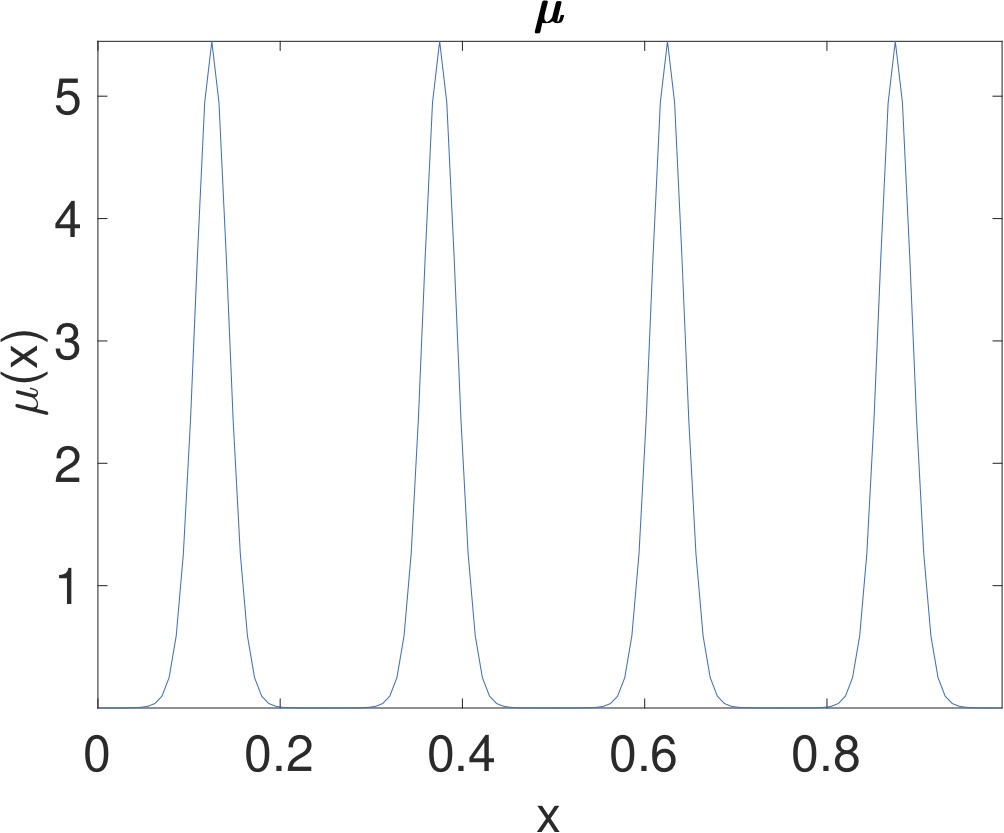
In this section, we demonstrate the properties of the newly derived equations with several examples. Since the gradient flow equations are linear, the flow dynamics are governed mostly by the spectrum of the Kolmogorov forward and backward operators. Here, we consider the simple setting of ΩΩ\Omega equal to the unit interval [0,1]01[0,1] with periodic boundary condition. The PDEs are numerically discretized with a finite element method with a uniform discretization.
Refer to caption Refer to caption Refer to caption
(a) (b) (c)
Refer to caption Refer to caption Refer to caption
(d) (e) (f)
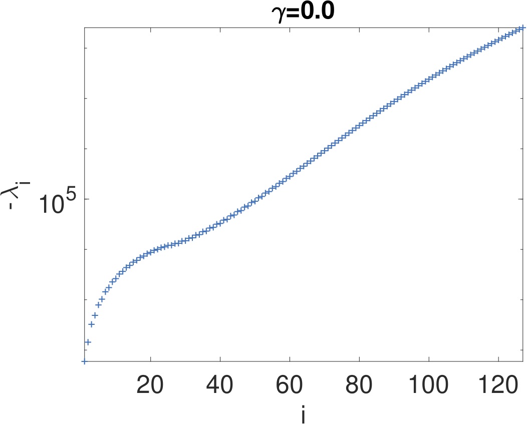
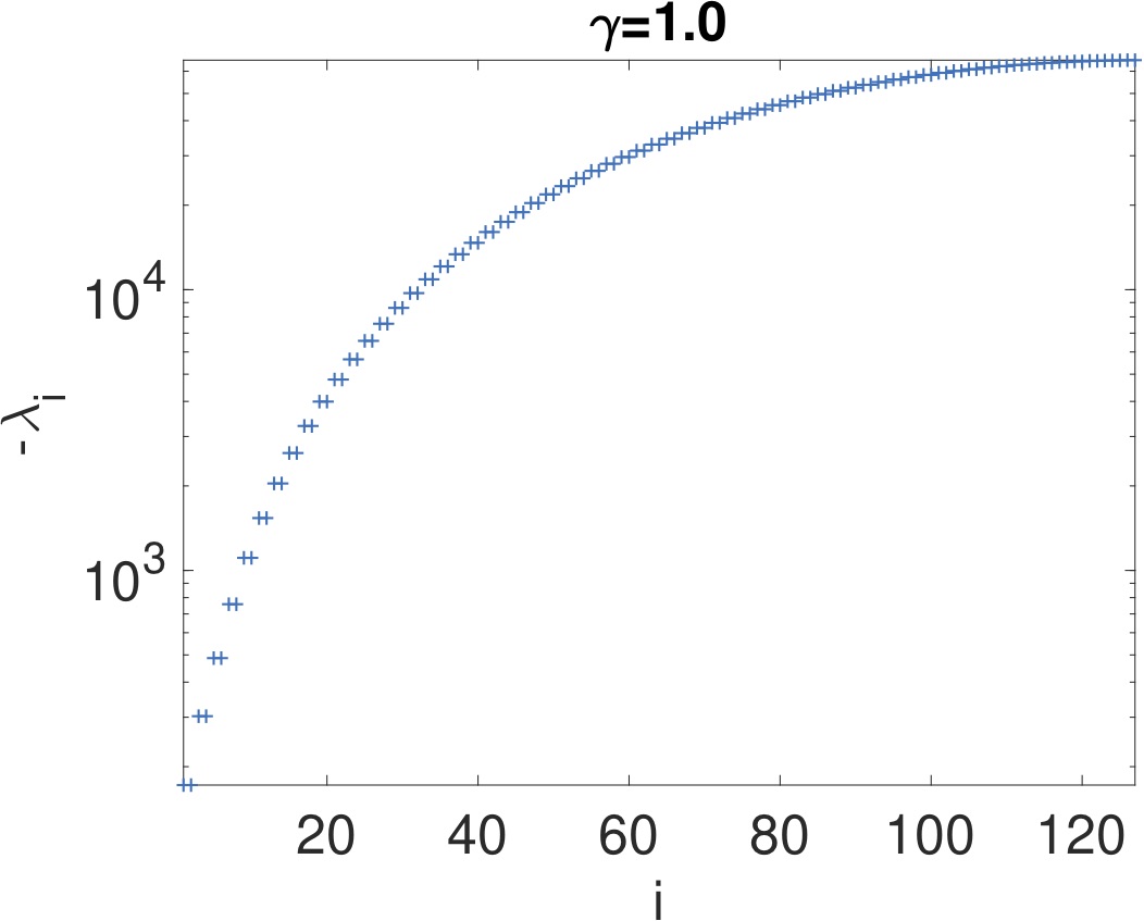
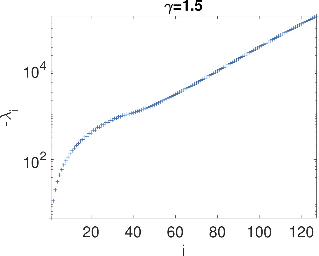
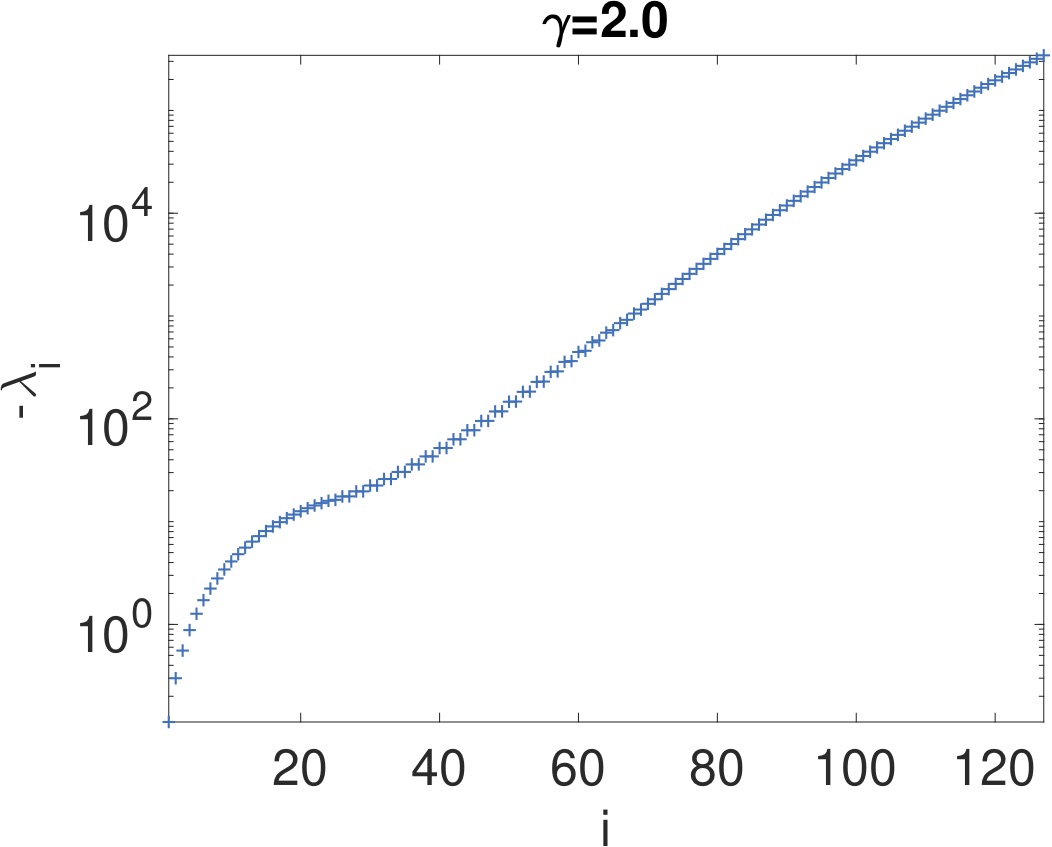
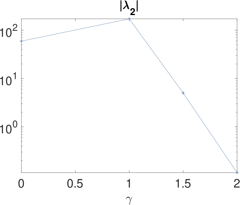
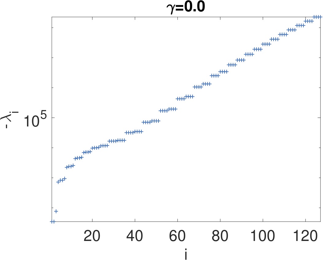
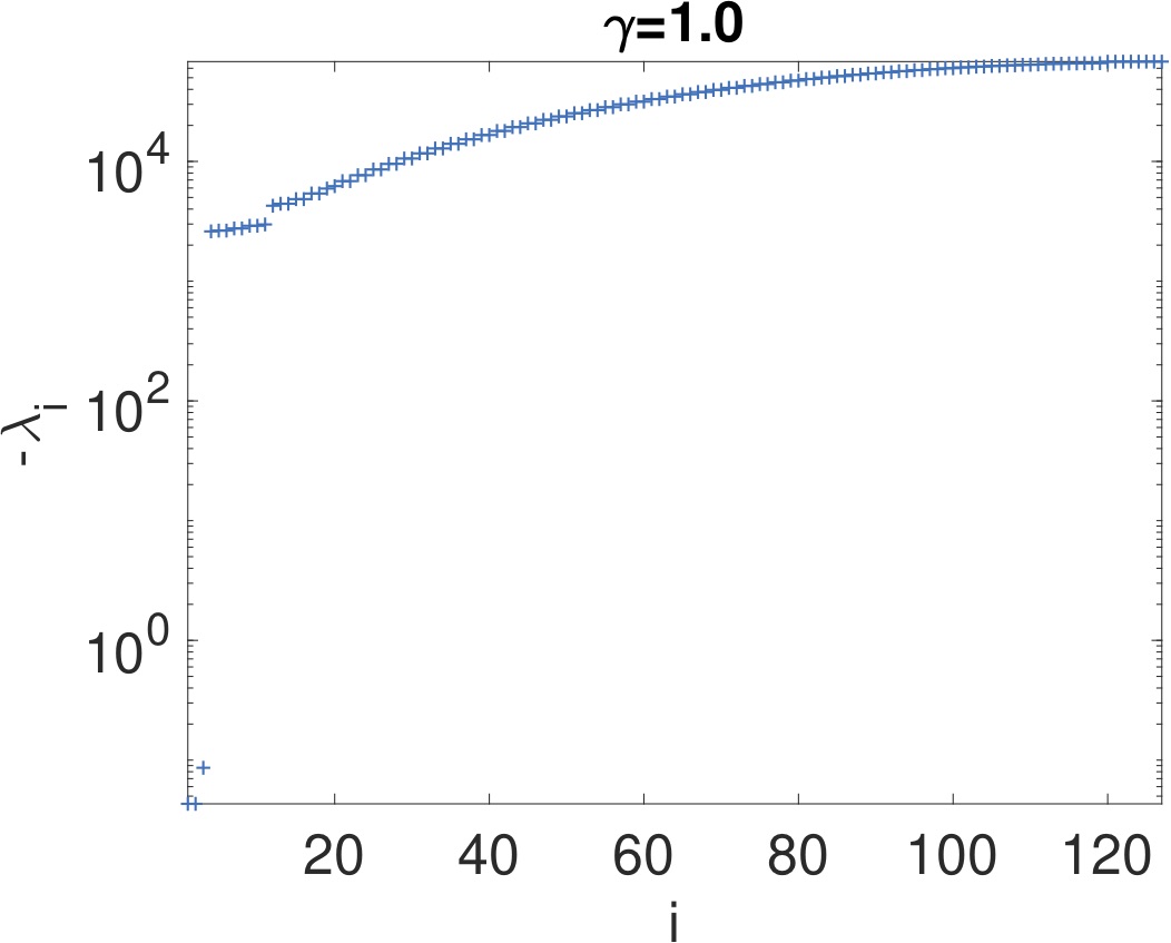
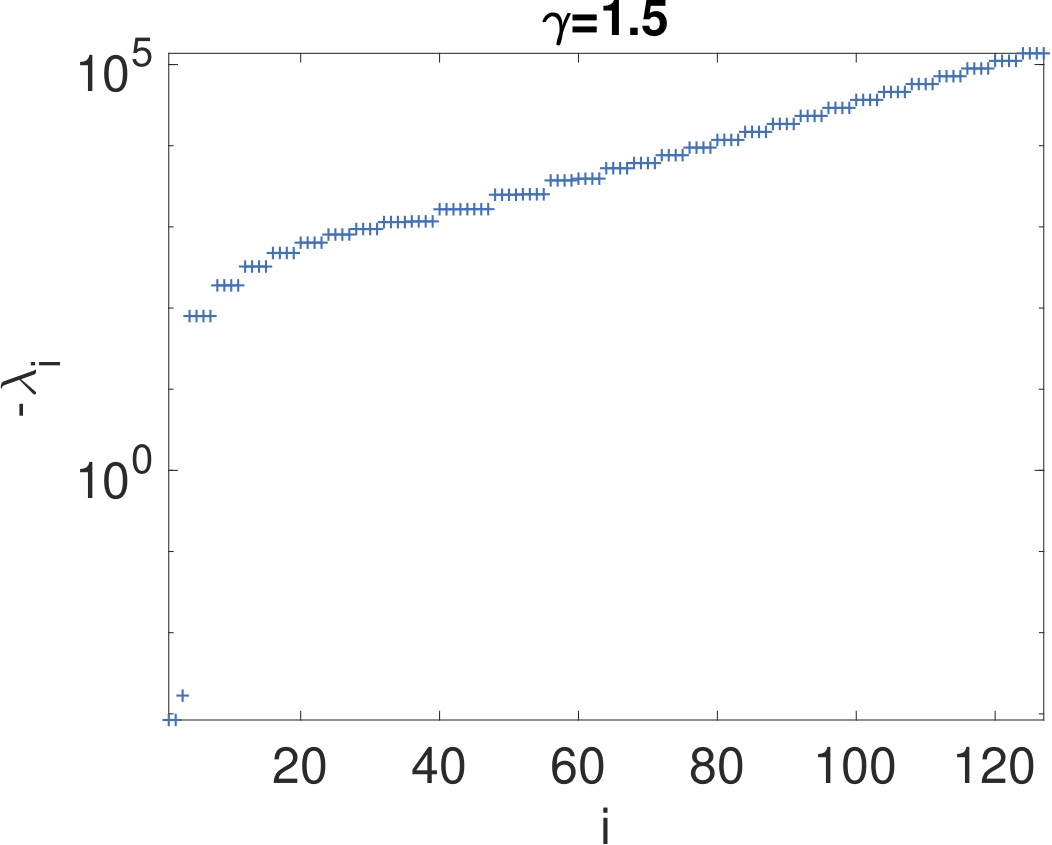
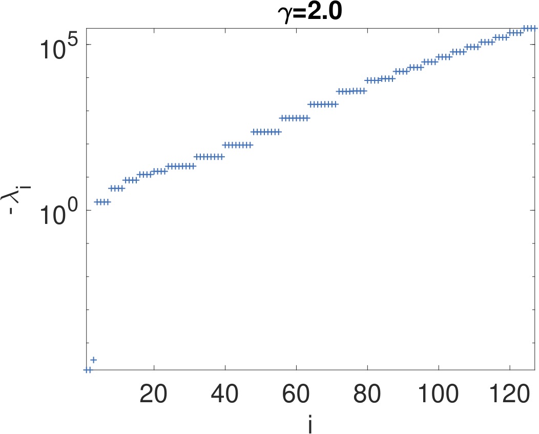
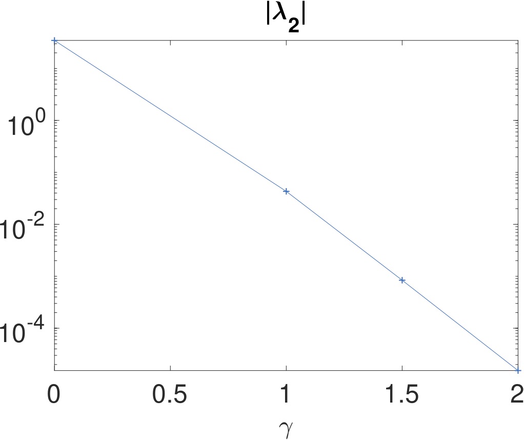
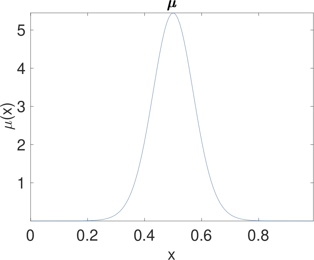
Figure 2. Unimodal case. (a) Reference measure μ(x)𝜇𝑥\mu(x). (b)-(e): The spectrum (part close to the zero) in the log-scale for the gradient flow PDEs with γ=0,1,1.5,2𝛾011.52\gamma=0,1,1.5,2. (f): The smallest non-zero eigenvalue λ2subscript𝜆2\lambda_{2} for the gradient flow PDEs with different choices of γ𝛾\gamma.

We consider two simple examples in this setting. In the first example, the reference measure μ(x)𝜇𝑥\mu(x) is a unimodal distribution (shown in Figure 2(a)). Figure 2 (b)-(e) plot the bottom part of the spectrum of the gradient flow PDEs for γ=0,1,1.5,2𝛾011.52\gamma=0,1,1.5,2. These γ𝛾\gamma values correspond to the Pearson, KL, Hellinger, and reverse KL divergence. We also summarize the magnitude of the smallest non-zero eigenvalue λ2subscript𝜆2\lambda_{2} for these choices of γ𝛾\gamma in Figure 2(f). For these linear gradient flow PDEs, |λ2|subscript𝜆2|\lambda_{2}| controls the convergence rate to the reference measure μ(x)𝜇𝑥\mu(x) for a generic initial condition ρ(t=0)𝜌𝑡0\rho(t=0). The plot suggests that among various choices of γ𝛾\gamma, the standard Fokker-Planck equation (γ=1𝛾1\gamma=1) has the largest |λ2|subscript𝜆2|\lambda_{2}| and hence the fastest convergence rate.
Refer to caption Refer to caption Refer to caption
(a) (b) (c)
Refer to caption Refer to caption Refer to caption
(d) (e) (f)
Figure 3. Multimodal case. (a) Reference measure μ(x)𝜇𝑥\mu(x). (b)-(e): The spectrum (part close to the zero) in the log-scale for the gradient flow PDEs with γ=0,1,1.5,2𝛾011.52\gamma=0,1,1.5,2. (f): The smallest non-zero eigenvalue λ2subscript𝜆2\lambda_{2} for the gradient flow PDEs with different choices of γ𝛾\gamma.

In the second example, the reference measure μ(x)𝜇𝑥\mu(x) is a multimodal distribution (shown in Figure 3(a)). Figure 3 (b)-(e) plot the bottom part of the spectrum of the gradient flow PDEs for γ=0,1,1.5,2𝛾011.52\gamma=0,1,1.5,2. We again summarize the magnitude of the smallest non-zero eigenvalue λ2subscript𝜆2\lambda_{2} for these choices of γ𝛾\gamma in Figure 3(f). It is a well-known fact that, for the multimodal distribution, there exists a gap between the first few lowest eigenvalues (the number of which is equal to the number of modes) and the rest of the spectrum, due to the metastable states. For the standard Fokker-Planck equation (γ=1𝛾1\gamma=1), this gap is shown clearly in (Figure 3(d)). From the plots in Figure 3, one can make two observations concerning the gradient flow PDEs introduce in Section 2. The first is that, although the gap seems to persist for γ𝛾\gamma greater than 111, it decreases when γ𝛾\gamma increases from 111. For example in Figure 3 the gap is significantly smaller at γ=0𝛾0\gamma=0. The second observation is that, in contrast to the unimodal case, |λ2|subscript𝜆2|\lambda_{2}| for the multimodal case is no longer obtained at γ=1𝛾1\gamma=1. In fact |λ2|subscript𝜆2|\lambda_{2}| increases quite rapidly as γ𝛾\gamma decreases from 111, thus implying that the gradient flow PDE of the Pearson (γ=0𝛾0\gamma=0) divergence converges at a faster rate compared to the one of the standard Fokker-Planck equation (γ=1𝛾1\gamma=1).

5. Discussions

In this paper, we propose a family of Riemannian metrics in the probability space, named Hessian transport metric. We demonstrate that the heat flow is the gradient flow of several energy functions under the HT-metrics. Following this, we further introduce the gradient flows of divergence functions in the HT-metrics, which can be interpreted as Kolmogorov forward equations of the associated HT-SDEs.

Our study is the first step to bridge Hessian geometry, Wasserstein geometry, and divergence functions. Several fundamental questions arise. Firstly, there are many entropies and divergence functions in information theory [1]. Besides the α𝛼\alpha divergences and α𝛼\alpha entropy, which type of entropy’s HT gradient flows of divergence functions are probability transition equations of HT-SDEs? Secondly, in machine learning applications, especially the parametric statistics, our new geometry structure leads to a new class of metrics in parameter spaces/statistical manifold. We expect some of these metrics will help the training process [16, 20].

References

  • [1] S. Amari. Information Geometry and Its Applications. Springer Publishing Company, Incorporated, 1st edition, 2016.
  • [2] S. Amari and A. Cichocki. Information geometry of divergence functions. Bulletin of the Polish Academy of Sciences: Technical Sciences, 58(1):183–195, 2010.
  • [3] S. Amari, R. Karakida, and M. Oizumi. Information Geometry Connecting Wasserstein Distance and Kullback-Leibler Divergence via the Entropy-Relaxed Transportation Problem. arXiv:1709.10219 [cs, math], 2017.
  • [4] A. Arnold, P. Markowich, G. Toscani, and A. Unterreiter. On convex Sobolev inequalities and the rate of convergence to equilibrium for Fokker-Planck type equations. Communications in Partial Differential Equations, 26(1-2):43–100, 2001.
  • [5] N. Ay, J. Jost, H. V. Lê, and L. Schwachhöfer. Information geometry, volume 64. Springer, Cham, 2017.
  • [6] M. Bauer, S. Joshi, and K. Modin. Diffeomorphic Density Matching by Optimal Information Transport. SIAM Journal on Imaging Sciences, 8(3):1718–1751, 2015.
  • [7] M. Bauer and K. Modin. Semi-invariant Riemannian metrics in hydrodynamics. arXiv:1810.03424 [math], 2018.
  • [8] Y. Cao, J. Lu, and Y. Lu. Exponential decay of Renyi divergence under Fokker-Planck equations. arXiv:1805.06554 [math], 2018.
  • [9] L. Chizat, G. Peyré, B. Schmitzer, and F.-X. Vialard. An Interpolating Distance Between Optimal Transport and Fisher–Rao Metrics. Foundations of Computational Mathematics, 18(1):1–44, 2018.
  • [10] S.-N. Chow, W. Li, and H. Zhou. Entropy dissipation of Fokker-Planck equations on graphs. Discrete & Continuous Dynamical Systems, series A, 2018.
  • [11] T. M. Cover and J. A. Thomas. Elements of Information Theory. Wiley Series in Telecommunications. Wiley, New York, 1991.
  • [12] I. Csiszár and P. C. Shields. Information Theory and Statistics: A Tutorial. Foundations and Trends™ in Communications and Information Theory, 1(4):417–528, 2004.
  • [13] R. Jordan, D. Kinderlehrer, and F. Otto. The variational formulation of the Fokker-Planck equation. SIAM J. Math. Anal., 29(1):1–17, 1998.
  • [14] J. D. Lafferty. The density manifold and configuration space quantization. Transactions of the American Mathematical Society, 305(2):699–741, 1988.
  • [15] W. Li. Geometry of probability simplex via optimal transport. arXiv:1803.06360 [math], 2018.
  • [16] W. Li, A. T. Lin, and G. Montufar. Affine natural proximal learning. Geometric science of information, 2019, 2019.
  • [17] W. Li and G. Montúfar. Natural gradient via optimal transport. Information Geometry, 1(2):181–214, Dec 2018.
  • [18] W. Li and G. Montufar. Ricci curvature for parametric statistics via optimal transport. CAM report 18-52, 2018.
  • [19] M. Liero, A. Mielke, and G. Savaré. Optimal entropy-transport problems and a new Hellinger-Kantorovich distance between positive measures. Invent. Math., 211(3):969–1117, 2018.
  • [20] A. T. Lin, W. Li, S. Osher, and G. Montufar. Wasserstein proximal of GANs. CAM report 18-53, 2019.
  • [21] Q. Liu. Stein variational gradient descent as gradient flow. In I. Guyon, U. V. Luxburg, S. Bengio, H. Wallach, R. Fergus, S. Vishwanathan, and R. Garnett, editors, Advances in Neural Information Processing Systems 30, pages 3115–3123. Curran Associates, Inc., 2017.
  • [22] Q. Liu and D. Wang. Stein variational gradient descent: A general purpose bayesian inference algorithm. In Proceedings of the 30th International Conference on Neural Information Processing Systems, NIPS’16, pages 2378–2386. Curran Associates Inc., USA, 2016.
  • [23] J. Lu, Y. Lu, and J. Nolen. Scaling limit of the stein variational gradient descent: The mean field regime. SIAM Journal on Mathematical Analysis, 51(2):648–671, 2019.
  • [24] L. Malagò, L. Montrucchio, and G. Pistone. Wasserstein Riemannian geometry of positive definite matrices. arXiv:1801.09269 [math, stat], 2018.
  • [25] H. Q. Minh. A unified formulation for the Bures-Wasserstein and Log-Euclidean/Log-Hilbert-Schmidt distances between positive definite operators. Geometry science of Information, 2019.
  • [26] E. Nelson. Quantum Fluctuations. Princeton Series in Physics. Princeton University Press, Princeton, N.J, 1985.
  • [27] B. K. Oksendal. Stochastic Differential Equations: An Introduction with Applications. Universitext. Springer, Berlin Heidelberg New York Dordrecht London, sixth edition, sixth corrected printing edition, 2013.
  • [28] F. Otto. The geometry of dissipative evolution equations the porous medium equation. Communications in Partial Differential Equations, 26(1-2):101–174, 2001.
  • [29] G. A. Pavliotis. Stochastic processes and applications, volume 60 of Texts in Applied Mathematics. Springer, New York, 2014. Diffusion processes, the Fokker-Planck and Langevin equations.
  • [30] D. Shlyakhtenko. Free Fisher Information for Non-Tracial States. arXiv:math/0101137, 2001.
  • [31] C. Tsallis. Possible generalization of boltzmann-gibbs statistics. Journal of Statistical Physics, 52(1):479–487, Jul 1988.
  • [32] C. Villani. Optimal Transport: Old and New. Number 338 in Grundlehren Der Mathematischen Wissenschaften. Springer, Berlin, 2009.
  • [33] T.-K. L. Wong. Logarithmic divergences from optimal transport and Renyi geometry. arXiv:1712.03610 [cs, math, stat], 2017.
  • [34] S. Zozor and J.-M. Brossier. deBruijn identities: From Shannon, Kullback-Leibler and Fisher to generalized ϕitalic-ϕ\phi-entropies, ϕitalic-ϕ\phi-divergences and ϕitalic-ϕ\phi-Fisher informations. AIP Conference Proceedings, 1641(1):522–529, 2015.