Deep Learning: a new definition of artificial neuron with double weight

Abstract

Deep learning is a subset of a broader family of machine learning methods based on learning data representations. These models are inspired by human biological nervous systems, even if there are various differences pertaining to the structural and functional properties of biological brains. The elementary constituents of deep learning models are neurons, which can be considered as functions that receive inputs and produce an output that is a weighted sum of the inputs fed through an activation function. Several models of neurons were proposed in the course of the years that are all based on learnable parameters called weights. In this paper we present a new type of artificial neuron, the double-weight neuron, characterized by additional learnable weights that lead to a more complex and accurate system. We tested a feed-forward and convolutional neural network consisting of double-weight neurons on the MNIST dataset, and we tested a convolution network on the CIFAR-10 dataset. For MNIST we find a $\approx 4\%$ and $\approx 1\%$ improved classification accuracy, respectively, when compared to a standard feed-forward and convolutional neural network built with the same sets of hyperparameters. For CIFAR-10 we find a $\approx 12\%$ improved classification accuracy. We thus conclude that this novel artificial neuron can be considered as a valuable alternative to common ones.

Keywords: Deep Learning, Machine Learning, Neural Networks, Artificial neurons, AI

1 Introduction

In the last few years there has been a revolutionary improvement in the fields of Artificial Intelligence (AI), Machine Learning (ML) and Deep Learning (DL). In particular, DL achieved the state-of-the-art on imaging classifications, (e.g., Dieleman et al., 2015; Nguyen, Clune, Bengio, Dosovitskiy & Yosinski, 2016; Katebi et al., 2018), and natural language processing (e.g., Young et al., 2017), while both ML and DL are now commonly used in physics, biology, and astronomy (e.g., Baldeschi et al., 2017; Schawinski et al., 2017; Zingales & Waldmann, 2018; Leung & Bovy, 2019; Reiman & Göhre, 2019) typically to tackle complex classification problems.

DL enables models, which are composed of several hidden layers, to learn representations of data with several degrees of abstraction. DL discovers hidden patterns in large datasets by adjusting the weights, which are commonly found by minimizing a loss function through the method of Gradient Descent (GD) or through some of its variants, such as Adam or Adadelta (Kingma & Ba, 2014).

Standard neural networks (NN) consist of artificial neurons, which are mathematical functions that receive one or more inputs and sum them to produce an output. Usually each input is separately weighted, and the sum is passed through a non-linear activation function.

In this paper we present a novel neuron architecture where an input value is double weighted, and we demonstrate that this new paradigm results in an improvement with respect to ordinary neurons. In particular, we show that a NN consisting of double-weight neurons produces improved classification accuracy when compared with an ordinary NN, with the same hyperparameters that characterize the NN.

This paper is organized as follows: in Section 2 we present the double-weight neuron, and in Section 3 we test our architecture on the the MNIST and CIFAR-10 datasets. Conclusions are drawn in Section 4.

2 The double-weight neuron

A standard artificial neuron is a function that receives inputs and produces an output according to the formula:

$$\hat{y}=\phi\big{(}\sum\limits_{i=1}^{m}w_{i}x_{i}+b\big{)},$$ (1)

where $\hat{y}$ is the output of the neuron, $x_{i}$ represents the inputs, $w_{i}$ and $b$ are the learnable weights and biases, respectively, $m$ is the number of inputs, and $\phi(\cdot)$ is an activation function.

The idea to add additional weights was already discussed in Arora et al. (2018) for linear NN. Here we add additional weights within a nonlinear NN.

We define the double-weight neuron as:

$$\hat{y}=\phi\big{(}\sum\limits_{i=1}^{m}\gamma_{i}w_{i}x_{i}+b\big{)},$$ (2)

where $\gamma_{i}$ are a set of additional learnable weights. From equation 2 the output values of a NN layer can be expressed by using the matrix notation:

$$\vec{y}=\phi((W*\Gamma)\vec{x}+\vec{b}),$$ (3)

where $\vec{x}$ is the input vector of size ($m\times 1$), $\vec{y}$ is the output vector of size ($k\times 1$), $\vec{b}$ is the bias vector of size ($k\times 1$) while $\Gamma$ and $W$ are weight matrices of size ($k\times m$), where $m$ is the number of inputs and $k$ is the number of neurons in the considered layer of the NN. Here $W*\Gamma$ represents the element-wise product between the two weights matrix.

Adding a second weight matrix in the NN adds complexity to the NN architecture and increases the training time. However, as we demonstrate in Section 3, the double-weight neuron leads to an improved performance in terms of classification accuracy. The NN with double-weight neurons can be trained by minimizing a loss function with the method of GD. The gradient can be analytically calculated by using the backpropagation algorithm that is implemented in tensorflow. In Appendix B we derive the back-propagation equations for a double-weight feed-forward neural network.

3 Data analysis

In this section we test a Feed Forward Neural Network (FNN) and a Convolutional Neural Network (CNN) consisting of double-weight neurons on the MNIST dataset, which is a large database of handwritten digits commonly used for training image processing systems. MNIST contains 60000 training images and 10000 testing images. Furthermore, we tested a CNN on the CIFAR-10 dataset, which is constituted of 50000 training and 10000 testing images and 10 classes.

The scope of this section is to show that the introduction of double-weight neurons leads to an improved classification accuracy for the same set of hyperparameters of the NN. We emphasize that we are not trying to achieve state-of-the-art results for either MNIST and CIFAR-10, and hence, the hyperparameters of the NN are not optimized.

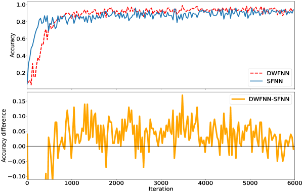
We start by comparing a Standard Feed-Forward Neural Network (SFNN) with a Double-Weight Feed-Forward Neural Network (DWFNN) on the MNIST dataset. A FNN is not well-suited for imaging classification problems, but here the scope is simply to compare a SFNN with a DWFNN, assuming the same set of hyperparameters. In figure 1, we show the classification accuracy as a function of the iteration number on the test set for the SFNN and DWFNN for the same set of hyperparameters that characterize the networks.

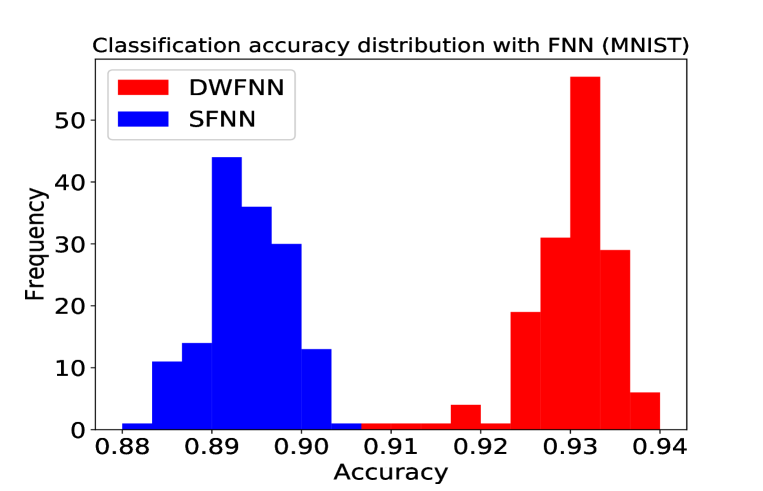
Since the cost function of a NN is not convex, for different initialization of the weights the GD minimization procedure leads to different local minima. Therefore, we tested a SFNN and a DWFNN for 150 random initial different weights configurations. For each realization we estimate the average of the classification accuracy, and then we build the distribution of the classification accuracy over the 150 realizations (see Fig. 2). The average values of the classification accuracy distribution for a SFNN and a DWFNN are 0.894 and 0.930, respectively. We also performed the Welch t-test for testing the significance of the difference between the mean values of the classification accuracy distribution for both SFNN and DWFNN, obtaining a highly significant p-value $<10^{-40}$. Figure 2, combined with the results of the Welch t-test demonstrates that the classification accuracy of a DWFNN is significantly better than the accuracy of a SFNN. The training time of a DWFNN is on average 1.46 times the training time of a SFNN for the MNIST dataset. A detailed description of the hyperparameters of the considered networks is presented in Appendix A.

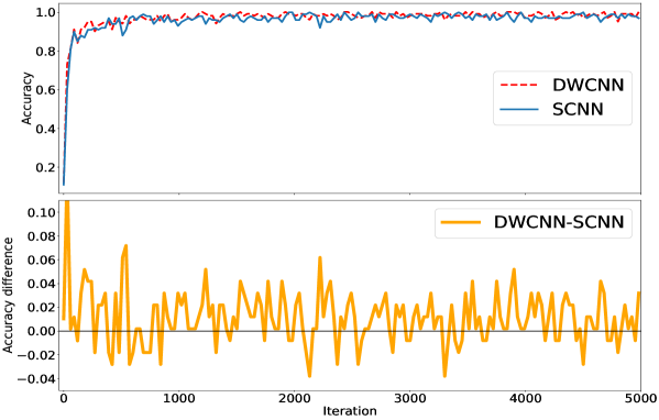
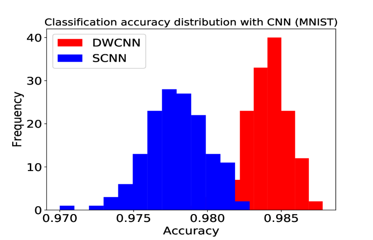
We also compared a CNN consisting of double-weight neurons (DWCNN) in the fully connected layers with a standard CNN (SCNN), repeating the same procedure as above. In Fig. 3 we show an example of classification accuracy as a function of the iteration number between a DWCNN and a SCNN. Figure 4 displays the results of the classification accuracy distribution, suggesting that a DWCNN is better than a SCNN. The mean values of the classification accuracy distribution of a DWCCN and SCNN are 0.978 and 0.984, respectively, and the p-value of the Welch’s t-test is $<10^{-40}$. The training time of a DWCNN is on average 1.11 times the training time of a SCNN for MNIST.

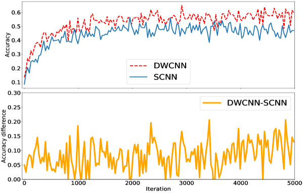
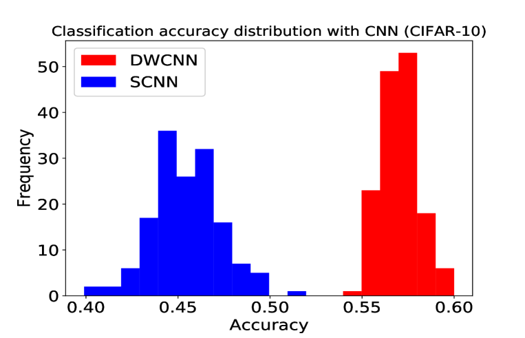
We also compared a DWCNN with a SCNN on CIFAR-10. In Fig. 5 we show an example of classification accuracy as a function of the iteration number between a DWCNN and a SCNN. Figure 6 shows the results of the classification accuracy distribution suggesting that a DWCNN is better than a SCNN. The mean values of the classification accuracy distribution of a DWCCN and SCNN are 0.570 and 0.455, respectively, and the p-value of the Welch t-test is $<10^{-40}$. The training time of a DWCNN is on average 1.07 times the training time of a SCNN for CIFAR-10.

The results of comparison between the networks are summarized in Table 1, and a detailed description of the CNN architectures is presented in Appendix A.

	MNIST	CIFAR-10
SFNN	0.894
DWFNN	0.930
SCNN	0.978	0.455
DWCNN	0.984	0.570

Table 1: Average value of the classification accuracy distribution for each of the considered NN architectures for both MNIST and CIFAR-10. The distribution was taken over 150 different random configurations of initial weights. The Welch t-test was used to test the null hypothesis that the standard NN and the double-weight NN have equal means, obtaining a p-value $<10^{-40}$ for either MNIST and CIFAR-10.

Figure 1: Upper panel: Classification accuracy as a function of the number of iterations for the MNIST dataset. Red dashed line: classification accuracy of the FNN with double weights (DWFNN) in the test set. Solid blue line: classification accuracy test set for the FNN with standard weights (SWFNN). Lower panel: difference between the red and blue curves as a function of the iteration. Average classification accuracy DWFNN: $\approx 0.93$. Average classification accuracy SWFNN: $\approx 0.89$. The average was taken by excluding the firsts 1500 iterations.

Figure 2: Classification accuracy distribution for the MNIST dataset using SFNN and DWFNN. The distribution was taken over 150 different random configurations of initial weights for both SFNN and DWFNN. In Table 1 we report the average values of the classification accuracy distribution for both SFNN and DWFNN. The p-value of the Welch t-test for the significance of the means is $<10^{-40}$.

Figure 3: Same as Fig. 1 but for the CNN. Average classification accuracy DWCNN: $\approx 0.99$. Average classification accuracy SCNN: $\approx 0.98$.

Figure 4: Same as Fig. 2 but for the CNN. The p-value of the Welch t-test for the significance of the means is $<10^{-40}$.

Figure 5: Same as Fig. 3 but for the CIFAR-10 dataset. Average classification accuracy DWCNN: $\approx 0.56$. Average classification accuracy SCNN: $\approx 0.47$.

Figure 6: Same as Fig. 4 but for the CIFAR-10 dataset. The p-value of the Welch t-test for the significance of the means is $<10^{-40}$.

4 Conclusions

In this paper we presented a new type of artificial neuron, the double-weight neuron, where we added learnable weights to the standard definition. We showed that a Feed-Forward Neural Network (FNN), built with these neurons and trained with the MNIST dataset, has on average $\approx 4\%$ larger mean classification accuracy than a standard FNN with the same hyperparameters that characterize the NN. We also tested a convolutional neural network (CNN) constituted by double-weight neurons in the fully connected layer only, on MNIST and CIFAR-10, and we found on average $\approx 1\%$ and $\approx 12\%$ improved classification accuracy, with respect to a standard CNN with the same set of hyperparameters.

These results suggest that a neural network built with double-weight neurons may be considered as a valuable alternative to the standard networks.

Acknowledgments

This work has been supported by the Heising-Simons Foundation under grant # 2018-0911 (PI: Margutti).

Appendix A.

In this appendix we describe the structure of the NNs presented in Section 3. The FNN for the MNIST dataset consist of four hidden layers and an output layer. The hidden layers are built in order with 200, 100, 60 and 30 neurons, respectively, while the output layer has 10 neurons. The learning rate is 0.003 and we used the Adam optimizer to minimize the cross entropy cost function. We fed 100 flattened images per iteration during training and testing. We used a sigmoid function as the activation function for the hidden layers and a softmax function for the output layer. We initialized the weights with a truncated normal of mean 0 and standard deviation of 0.1, while we initialized the biases with zeros. The only difference between the DWFNN and SFNN is the presence of double-weight neurons in the DWFNN.

The CNN, for the MNIST dataset consist of 3 convolutional layers, 2 fully connected layers, and an output layer. The output depth of the convolutional and fully connected layers are 4, 8, 12, 200 and 80, respectively. The convolutional window is $5\times 5$ for the first and second convolutional layers, while it is $4\times 4$ for the third convolutional layer. The adopted stride for the first convolutional layer is 1, while a value of 2 was adopted for the second and third convolutional layers. We used the keyword ’SAME’ for the padding in tensorflow. The weights were initialized with a truncated normal of mean 0 and standard deviation of 0.1. The learning rate is 0.0008 and we used the Adam optimizer to minimize the cross entropy cost function. We fed 100 images per iteration during training and testing. We used a rectified linear activation function (RELU) for the hidden layers and a softmax function for the output layer. The only difference between the DWCNN and SCNN is the presence of the double-weight neurons in the fully connected layers in the DWCNN. The CNN architecture for CIFAR-10 is the same as of that used for MNIST, with the only differences being the learning rate (which we set equal to 0.0006) and the number of images processed per iteration, which we set equal to 200.

Appendix B.

In this appendix we derive the back-propagation formulas for a DWFNN. We consider a DWFNN with one hidden layer and a sum of square residuals cost function.

Considering the following equations:

$$E=\frac{1}{2}\sum_{j}\big{(}y_{j}-\hat{y}_{j}^{l}\big{)}^{2}$$ (4)

$$\hat{y}_{j}^{l}=\phi(z_{j}^{l})$$ (5)

$$z_{j}^{l}=\sum_{i}w_{ji}^{l}\gamma_{ji}^{l}\hat{y}_{j}^{l-1}$$ (6)

$$\hat{y}_{k}^{l-1}=\phi(z_{k}^{l-1})$$ (7)

$$z_{k}^{l-1}=\sum_{s}w_{ks}^{l-1}\gamma_{ks}^{l-1}\hat{y}_{s}^{l-2}$$ (8)

Where $E$ is the sum of square residuals cost function, $y_{j}$ represents the target values in the j neuron, $\hat{y}_{j}^{l}$ represents the output values of the $j$ neuron in the $l$ layer of the NN , $w_{ji}^{l}$ and $\gamma_{ji}^{l}$ are the weights between the hidden layer and the output layer, $\hat{y}_{k}^{l-1}$ is the output of the $k$ neuron in the $l-1$ layer, while $\gamma_{ks}^{l-1}$ and $w_{ks}^{l-1}$ are the weights between the $l-2$ and $l-1$ layer. These equations define the forward propagation in the NN.

The gradient of $E$ for the weights between the $l-1$ and $l$ layer is:

$$\frac{\partial E}{\partial w_{ji}^{l}}=\frac{\partial E}{\partial\hat{y}_{j}^{l}}\frac{\partial\hat{y}_{j}^{l}}{\partial z_{j}^{l}}\frac{\partial z_{j}^{l}}{\partial w_{ji}^{l}}=\big{(}\hat{y}_{j}^{l}-y_{j}\big{)}\phi^{\prime}(z_{j}^{l})\gamma_{ji}^{l}\hat{y}_{i}^{l-1},$$ (9)

and

$$\frac{\partial E}{\partial\gamma_{ji}^{l}}=\big{(}\hat{y}_{j}^{l}-y_{j}\big{)}\phi^{\prime}(z_{j}^{l})w_{ji}^{l}\hat{y}_{i}^{l-1}.$$ (10)

The estimate of the gradient for the weights between the input and $l-1$ layer is:

$$\frac{\partial E}{\partial w_{ks}^{l-1}}=-\sum_{j}\big{(}y_{j}-\hat{y}_{j}^{l}\big{)}\frac{\partial\hat{y}_{j}^{l}}{\partial z_{j}^{l}}\frac{\partial z_{j}^{l}}{\partial\hat{y}_{k}^{l-1}}\frac{\partial\hat{y}_{k}^{l-1}}{\partial z_{k}^{l-1}}\frac{\partial z_{k}^{l-1}}{\partial\hat{w}_{ks}^{l-1}}.$$ (11)

Eq. 11 can be expressed as:

$$\frac{\partial E}{\partial w_{ks}^{l-1}}=-\phi^{\prime}(z_{k}^{l-1})\gamma_{ks}^{l-1}\hat{y}_{s}^{l-2}\sum_{j}\big{(}y_{j}-\hat{y}_{j}^{l}\big{)}\phi^{\prime}(z_{j}^{l})\gamma_{jk}^{l}w_{jk}^{l},$$ (12)

similarly, we obtain:

$$\frac{\partial E}{\partial\gamma_{ks}^{l-1}}=-\phi^{\prime}(z_{k}^{l-1})w_{ks}^{l-1}\hat{y}_{s}^{l-2}\sum_{j}\big{(}y_{j}-\hat{y}_{j}^{l}\big{)}\phi^{\prime}(z_{j}^{l})\gamma_{jk}^{l}w_{jk}^{l}.$$ (13)

Equations 9, 10, 12 and 13 are the back-propagation equations for a DWFNN.

References

- Leung & Bovy (2019) Leung, H. W., & Bovy, J. 2019, MNRAS, 483, 3255
- Baldeschi et al. (2017) Baldeschi, A., Elia, D., Molinari, S., et al. 2017, MNRAS, 466, 3682
- Sabour et al. (2017) Sabour, S., Frosst, N., & E Hinton, G. 2017, arXiv:1710.09829
- Kingma & Ba (2014) Kingma, D. P., & Ba, J. 2014, arXiv:1412.6980
- Dieleman et al. (2015) Dieleman, S., Willett, K. W., & Dambre, J. 2015, MNRAS, 450, 1441
- Katebi et al. (2018) Katebi, R., Zhou, Y., Chornock, R., & Bunescu, R. 2018, arXiv:1809.08377
- Young et al. (2017) Young, T., Hazarika, D., Poria, S., & Cambria, E. 2017, arXiv:1708.02709
- Schawinski et al. (2017) Schawinski, K., Zhang, C., Zhang, H., Fowler, L., & Santhanam, G. K. 2017, MNRAS, 467, L110
- Nguyen, Clune, Bengio, Dosovitskiy & Yosinski (2016) Nguyen A., Clune J., Bengio Y., Dosovitskiy A., Yosinski J., 2016, arXiv e-prints, arXiv:1612.00005
- Zingales & Waldmann (2018) Zingales, T., & Waldmann, I. P. 2018, apj, 156, 268
- Reiman & Göhre (2019) Reiman, D. M., & Göhre, B. E. 2019, MNRAS, 485, 2617
- Arora et al. (2018) Arora, S., Cohen, N., & Hazan, E. 2018, arXiv:1802.06509