Deep Plug-and-Play Prior for Low-Rank Tensor Completion

Abstract

Multi-dimensional images, such as color images and multi-spectral images, are highly correlated and contain abundant spatial and spectral information. However, real-world multi-dimensional images are usually corrupted by missing entries. By integrating deterministic low-rankness prior to the data-driven deep prior, we suggest a novel regularized tensor completion model for multi-dimensional image completion. In the objective function, we adopt the newly emerged tensor nuclear norm (TNN) to characterize the global low-rankness prior of the multi-dimensional images. We also formulate an implicit regularizer by plugging into a denoising neural network (termed as deep denoiser), which is convinced to express the deep image prior learned from a large number of natural images. The resulting model can be solved by the alternating directional method of multipliers algorithm under the plug-and-play (PnP) framework. Experimental results on color images, videos, and multi-spectral images demonstrate that the proposed method can recover both the global structure and fine details very well and achieve superior performance over competing methods in terms of quality metrics and visual effects.

1 Introduction

The image completion problem aims to estimate missing entries from the partially observed entries, which is a fundamental problem in low-level computer vision and computational imaging [1, 2, 3, 4, 5, 6, 7, 8].

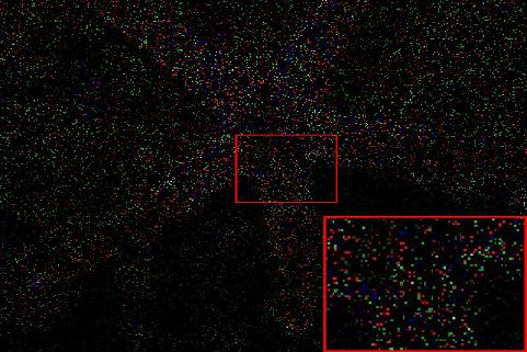
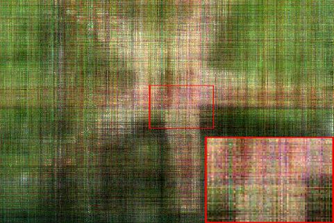
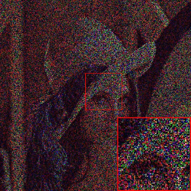
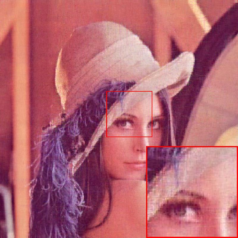
Observed (PSNR 2.03 dB)	SNN (PSNR 15.47 dB)
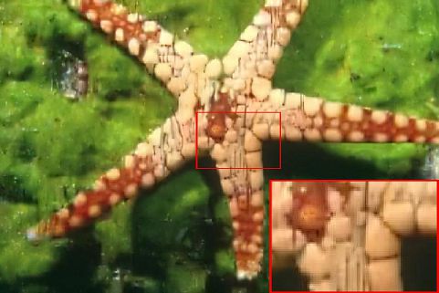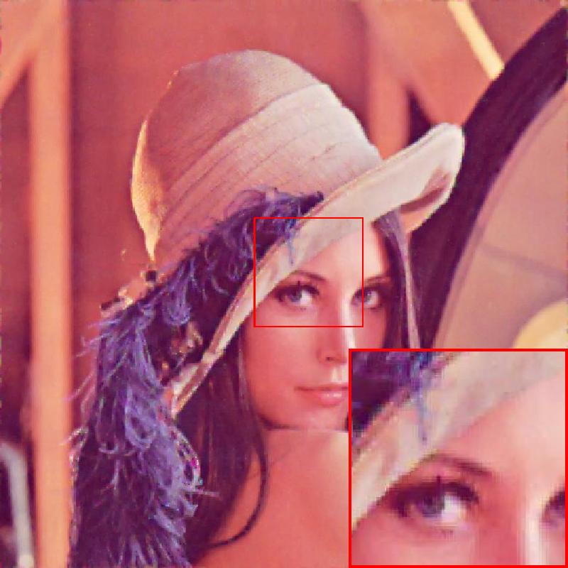
TNN (PSNR 15.73 dB)	DP3LRTC (PSNR 23.77 dB)

Figure 1: The recovered results by SNN, TNN, and the poposed DP3LRTC on color image Starfish with the sampling rate $5\%$ .

By exploiting the redundancy of natural images, the image completion problem can be formulated as the following low-rank matrix completion (LRMC) model:

$$\arg\min_{{\mathbf{X}}}\ \text{rank}({\mathbf{X}})\quad\text{s.t.}\ \mathcal{P}_{\Omega}({\mathbf{X}})=\mathcal{P}_{\Omega}({\mathbf{O}}),$$ (1)

where ${\mathbf{X}}$ is the underlying matrix, $\mathcal{\mathbf{O}}$ is the observed incomplete matrix, $\Omega$ is the index set corresponding to the observed entries, $\mathcal{P}_{\Omega}(\cdot)$ is the projection function that keeps the entries in $\Omega$ while setting others be zeros, and the elements of the observation $\mathbf{O}$ in the set $\Omega$ are given while the remaining elements are missing. For gray images, the low-rankness is characterized by the matrix rank or its convex envelope, i.e., the nuclear norm. For multi-dimensional images, the image elements are usually reordered into a matrix, which is known as matricization or unfolding.

However, matricization will inevitably destroy the intrinsic structure of multi-dimensional images. As the higher-order extension of the matrix, the tensor can provide a more natural and compact representation for multi-dimensional images. Thus we can formulate the image completion problem as the following low-rank tensor completion (LRTC) model:

$$\arg\min_{\mathcal{X}}\ \text{rank}(\mathcal{X})\quad\text{s.t.}\ \mathcal{P}_{\Omega}(\mathcal{X})=\mathcal{P}_{\Omega}(\mathcal{O}),$$ (2)

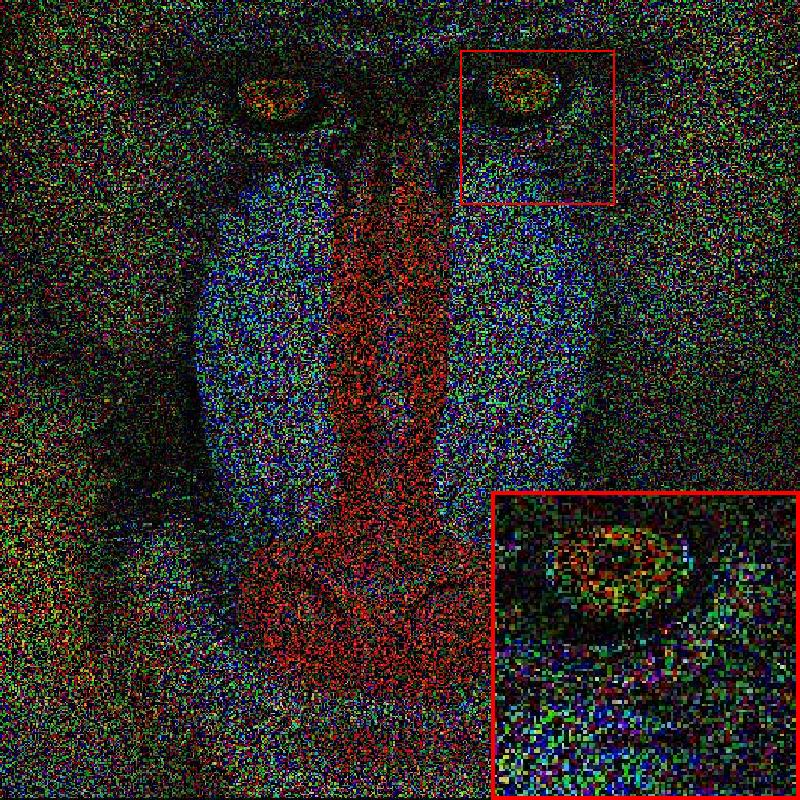
where $\mathcal{X}$ is the underlying tensor and $\mathcal{O}$ is the observed incomplete tensor (as shown in the top-left of Fig. 1). Here, we generally consider the element-wise sampling in the model (2), which can be extended to the structured sampling, e.g., inpainting [1] and demosaicing [9].

Different from the matrix case, there is not an exact (or unique) definition for tensor rank. Thus, how to define the tensor rank becomes an important task. Many research efforts have been devoted to this topic [10, 11, 12, 13], such as the CANDECOMP/PARAFAC (CP) rank and the Tucker rank. The CP rank is defined based on the CP decomposition, where an $n$-th order tensor is decomposed as the sum of rank-one tensors [14, 15], i.e., the outer product of $n$ vectors. The CP rank is defined as the minimal number of the rank-one tensors required to express the target tensor [16]. However, its related optimization is difficult, and even determining the CP rank of a given tensor is NP-hard [17]. The Tucker rank is based on the Tucker decomposition which decomposes a tensor into a core tensor multiplied by a matrix along each mode [18, 19, 20, 21]. The Tucker rank is defined as the vector consisting of the ranks of unfolding matrices. The Tucker rank has been considered in the LRTC problem by minimizing its convex surrogate, i.e., the sum of the nuclear norm (SNN) [18], or the non-convex surrogates[22, 23]. The top-right of Fig. 1 exhibits the recovered result by the SNN-based model. However, unfolding the tensor along each mode will also destroy the intrinsic structures of the tensor.

The tensor singular value decomposition (t-SVD), based on the tensor-tensor product (t-product), has been emerged as a powerful tool for preserving the intrinsic structures of the tensor [24, 25]. Although the t-SVD is originally suggested for third-order tensors, it has been extended to $n$-th order tensors ($n\geq 3$) [26, 27]. Based on the t-SVD, the corresponding multi-rank and tubal-rank have received considerable attention. The tensor nuclear norm (TNN) [28, 29, 30, 31, 32] is suggested as a convex surrogate of the multi-rank. The TNN-based LRTC model is given as follows:

$$\arg\min_{\mathcal{X}}\left\|\mathcal{X}\right\|_{\text{TNN}}\quad\text{s.t.}\quad\mathcal{P}_{\Omega}(\mathcal{X})=\mathcal{P}_{\Omega}(\mathcal{O}),$$ (3)

where $\mathcal{X}\in\mathbb{R}^{n_{1}\times n_{2}\times n_{3}}$, $\left\|\mathcal{X}\right\|_{\text{TNN}}=\sum_{i=1}^{n_{3}}\left\|\bar{\mathbf{X}}^{(i)}\right\|_{\ast}$, $\bar{\mathbf{X}}^{(i)}$ is the $i$-th frontal slice of $\mathcal{\bar{X}}$, and $\bar{\mathcal{X}}$ is the tensor generated by performing discrete Fourier transformation (DFT) along the mode-3 fibers (tubes) of $\mathcal{X}$, i.e., $\mathcal{\bar{X}}={\tt{fft}}(\mathcal{X},[],3)$. The TNN regularizer has the advantage of preserving the global structure of multi-dimensional images. We can observe from Fig. 1 that the recovered result by the TNN-based method (bottom-left) is slightly better than that by the SNN-based method (top-right).

Although promoting the low-rankness of the underlying data has shown its effectiveness for tensor completion, these methods suffer from two drawbacks. First, many real-world multi-dimensional images contain abundant fine details. This makes these multi-dimensional images are not strictly low-rank in mathematics. Second, when the sampling rate is extremely low or structurally sampled, the rank of these observed entries is already low. The low-rank regularization is insufficient for a fancy recovery of the underlying tensor. This phenomena can be observed in Fig.  1, where results by the SNN-based model and TNN-based model are low-quality when the sampling rate is 5%.

As a compensation, many LRTC methods introduce additional regularizers, which express other types of image priors, for a better solution of this ill-posed inverse problem. For example, the total variation (TV) regularizer, framelet regularizer, and nonlocal regularizer have received much attention [33, 34, 35, 36]. In particular, the TV regularizer was incorporated into the TNN-based LRTC model by exploiting the local smoothness [37]. Recently, deep learning-based methods have been developed to learn data-driven priors from a large number of natural images [38, 39, 40] and have shown promising performance on extensive application. Therefore, we consider to leverage the power of deep learning-based methods.

However, from the literatures, convolutional neural networks (CNNs) are successfully applied for the recovery of 2-D gray level images or the color images. There is not a general CNN structure suitable for various types of multi-dimensional imaging data. Fortunately, the multi-dimensional imaging data can be viewed as consisting of the typical 2-D gray level images. For example, each frame of a video is indeed a 2-D image and each band of a multi-spectral image looks also like a 2-D image. Thus, we believe that the CNNs designed for 2-D images can be utilized in LRTC.

In this work, we attempt to exploit the respective strengths of the deterministic low-rankness prior and the data-driven deep image prior. By integrating the low-rankness prior with deep image prior expressed by an implicit regularizer, we suggest the novel LRTC model as follows:

$$\arg\min_{\mathcal{X}}\left\|\mathcal{X}\right\|_{\text{TNN}}+\lambda\Phi(\mathcal{X})\quad\text{s.t.}\quad\mathcal{P}_{\Omega}(\mathcal{X})=\mathcal{P}_{\Omega}(\mathcal{O}),$$ (4)

where $\Phi(\mathcal{X})$ is an implicit regularizer to plug in the denoising CNNs (termed as deep denoisers). In (4), the two regularizers are organically combined and benefit from each other. On the one hand, the implicit regularizer can bring in deep image priors to each 2-D spatial slice of the multi-dimensional imaging data, well characterizing the fine details which can hardly be captured by the TNN regularizer. On the other hand, TNN can enforce the inner global correlations of the multi-dimensional imaging data, avoiding the lackness of lack inherent relations that the slices, which are separately handled by the CNN, . $\left\|\mathcal{X}\right\|_{\text{TNN}}$ and $\Phi(\mathcal{X})$ respectively regularize the coarse structure and the fine details, being complementary to each other. To efficiently solve the proposed model, we develop the alternating direction method of multipliers (ADMM) [41] under the highly flexible Plug-and-Play (PnP) framework [42, 43, 44], which allows us to plug in the stat-of-the-art deep denoisers. We term our method as deep plug-and-play prior for low-rank tensor completion (DP3LRTC). From the bottom-right of Fig. 1, we can observe that the deterministic low-rankness prior and data-driven deep image prior contribute to the superior performance of the proposed DP3LRTC.

The rest of this paper is organized as follows. Section 2 presents minimal preliminaries necessary for the subsequent discussion. Section 3 gives the corresponding solving algorithm to tackle the proposed model. Section 4 gives the experimental results and discusses details about the DP3LRTC. Section 5 concludes this paper.

2 Preliminaries

In this section, we introduce minimal and necessary preliminaries of the modular parts, i.e., TNN and PnP, for the subsequent discussion.

2.1 Notations

In this subsection, we give the basic notations and briefly introduce some definitions. We denote vectors as bold lowercase letters (e.g., $\mathbf{x}$), matrices as uppercase letters (e.g., $\mathbf{X}$), and tensors as calligraphic letters (e.g., $\mathcal{X}$). For a third-order tensor $\mathcal{X}\in\mathbb{R}^{n_{1}\times n_{2}\times n_{3}}$, with the MATLAB notation, we denote its $(i,j,k)$-th element as $\mathcal{X}(i,j,k)$ or $\mathcal{X}_{i,j,k}$. Its $(i,j)$-th mode-1, mode-2, and mode-3 fibers are denoted as $\mathcal{X}(:,i,j)$, $\mathcal{X}(i,:,j)$, and $\mathcal{X}(i,j,:)$, respectively. We use $\mathcal{X}(i,:,:)$, $\mathcal{X}(:,i,:)$, and $\mathcal{X}(:,:,i)$ to denote the $i$-th horizontal, lateral, and frontal slices of $\mathcal{X}$, respectively. More compactly, we also use $\mathbf{X}^{(i)}$ to represent the $i$-th frontal slices $\mathcal{X}(:,:,i)$. The Frobenius norm of $\mathcal{X}$ is defined as $\|\mathcal{X}\|_{F}:=\sqrt{\sum_{i,j,k}|\mathcal{X}(i,j,k)|^{2}}$.

2.2 T-SVD and TNN

Recently, Kilmer have introduced the novel tensor-tensor product as follows:

Definition 1 (t-product [25])

Let $\mathcal{A}$ be $n_{1}\times n_{2}\times n_{3}$ and $\mathcal{B}$ be $n_{2}\times n_{4}\times n_{3}$. Then the tensor-tensor product (t-product) is the $n_{1}\times n_{4}\times n_{3}$ tensor $\mathcal{C}=\mathcal{A}*\mathcal{B}$ whose $(i,j)$th tube is given by

$$\mathcal{C}(i,j,:)=\sum_{k=1}^{n_{2}}\mathcal{B}(i,k,:)\star\mathcal{C}(k,j,:),$$ (5)

where “$\star$" denotes circular convolution of two vectors.

Definition 2 (special tensors [25])

The conjugate transpose of a third-order tensor $\mathcal{X}\in\mathbb{R}^{n_{1}\times n_{2}\times n_{3}}$, denote as $\mathcal{X}^{\mathrm{H}}$, is the tensor obtained by conjugate transposing each of the frontal slices and then reversing the order of transposed frontal slices 2 through $n_{3}$. The identity tensor $\mathcal{I}\in\mathbb{R}^{n_{1}\times n_{2}\times n_{3}}$ is the tensor whose first frontal slice is the identity matrix, and other frontal slices are all zeros. A third-order tensor $\mathcal{Q}$ is orthogonal if $\mathcal{Q}\ast\mathcal{Q}^{\mathrm{H}}=\mathcal{Q}^{\mathrm{H}}\ast\mathcal{Q}=\mathcal{I}.$ A third-order tensor $\mathcal{S}$ is f-diagonal if each of its frontal slices is a diagonal matrix.

Based on t-product, the tensor singular value decomposition (t-SVD) is suggested.

Theorem 1 (t-SVD [25])

Let $\mathcal{X}\in\mathbb{R}^{n_{1}\times n_{2}\times n_{3}}$ be a third-order tensor, then it can be decomposed as

$$\mathcal{X}=\mathcal{U}\ast\mathcal{S}\ast\mathcal{V}^{\mathrm{H}},$$ (6)

where $\mathcal{U}\in\mathbb{R}^{n_{1}\times n_{1}\times n_{3}}$ and $\mathcal{V}\in\mathbb{R}^{n_{2}\times n_{2}\times n_{3}}$ are the orthogonal tensors, and $\mathcal{S}\in\mathbb{R}^{n_{1}\times n_{2}\times n_{3}}$ is a f-diagonal tensor whose frontal slices are diagonal matrices.

The t-SVD can be efficiently obtained by computing a series of matrix SVDs in the Fourier domain; see Algorithm 1 for more details.

Algorithm 1 The t-SVD for a third-order tensor.

1:$\mathcal{X}\in\mathbb{R}^{n_{1}\times n_{2}\times n_{3}}$.

2:$\bar{\mathcal{X}}\leftarrow$ $\tt{fft}$$(\mathcal{X},[],3)$.

3:for $i=1$ to $n_{3}$ do

4:     $[U,S,V]=$ $\tt{svd}$$(\bar{X}^{(i)})$.

5:     $\bar{U}^{(i)}\leftarrow U$; $\bar{S}^{(i)}\leftarrow S$; $\bar{V}^{(i)}\leftarrow V$.

6:end for

7:$\mathcal{U}\leftarrow$ $\tt{ifft}$$(\bar{\mathcal{U}},[],3)$.

8:$\mathcal{S}\leftarrow$ $\tt{ifft}$$(\bar{\mathcal{S}},[],3)$.

9:$\mathcal{V}\leftarrow$ $\tt{ifft}$$(\bar{\mathcal{V}},[],3)$.

10:$\mathcal{U}$, $\mathcal{S}$, $\mathcal{V}$.

Based on t-SVD, we have the corresponding definitions of tensor multi-rank and tubal-rank.

Definition 3 (tensor tubal-rank and multi-rank [28])

Let $\mathcal{X}\in\mathbb{R}^{n_{1}\times n_{2}\times n_{3}}$ be a third-order tensor, the tensor multi-rank, denoted as $\text{rank}_{\text{m}}(\mathcal{X})\in\mathbb{R}^{n_{3}}$, is a vector whose $i$-th element is the rank of the $i$-th frontal slice of $\bar{\mathcal{X}}$, where $\bar{\mathcal{X}}=\mathrm{\tt fft}(\mathcal{X},[],3)$. The tubal-rank of $\mathcal{X}$, denote as $\text{rank}_{\text{t}}(\mathcal{X})$, is defined as the number of non-zero tubes of $\mathcal{S}$, where $\mathcal{X}=\mathcal{U}\ast\mathcal{S}\ast\mathcal{V}^{\mathrm{H}}$.

The relationship between the tubal-rank and multi-rank is $\text{rank}_{\text{t}}(\mathcal{X})=\max\big{(}\text{rank}_{\text{m}}(\mathcal{X})\big{)}$. The convex surrogate of the multi-rank is suggested as follows:

Definition 4 (TNN [28])

The tensor nuclear norm of a tensor $\mathcal{X}\in\mathbb{R}^{n_{1}\times n_{2}\times n_{3}}$, denoted as $\|\mathcal{X}\|_{\text{TNN}}$, is defined as the sum of singular values of all the frontal slices of $\bar{\mathcal{X}}$, i.e.,

$$\left\|\mathcal{X}\right\|_{\text{TNN}}:=\sum_{i=1}^{n_{3}}\|\bar{\mathbf{X}}^{(i)}\|_{*}.$$ (7)

where $\bar{\mathbf{X}}^{(i)}$ is the $i$-th frontal slice of $\mathcal{\bar{X}}$, and $\bar{\mathcal{X}}=\mathrm{\tt fft}(\mathcal{X},[],3)$.

2.3 Plug-and-Play (PnP) Framework

PnP is a highly flexible framework [42, 43, 44] that leverages the power of the state-of-the-art denoisers in the ADMM or other proximal algorithms. After variable splitting technique, the optimization problem is decoupled into easier subproblems, one of which is the proximal operator of regularization. The proximal operator of regularization $\textrm{prox}_{\Phi}:\mathbb{R}^{n}\rightarrow\mathbb{R}^{n}$ is defined as

$$\textrm{prox}_{\Phi}(y)=\textrm{arg}\mathop{\textrm{min}}_{x}\left\{\Phi(x)+\frac{\rho}{2}\left\|x-y\right\|^{2}\right\},$$ (8)

which maps the input $y$ to the minimizer of (8). Under the PnP framework, the proximal operator of regularization is replaced by the denoising algorithm (termed as denoiser), which maps the noisy image to the clean image. Here the denoiser serves as an implicit regularizer to express the deep image prior. Regularization by Denoising (RED) [45, 46], which uses the denoising engine in defining the regularization of the inverse problem, is also suggested as an alternative framework.

The state-of-the-art denoisers can be flexibly plugged in as a modular part under the PnP framework. In the past decades, the hand-crafted denoisers, which exploit the deterministic priors of the nature images, have been dominantly used, e.g., TV denoiser [47], framelet denoiser [48], BM3D denoiser [49], WNNM denoiser [50], and ITS denoiser [51]. Recently, deep learning-based denoisers have been rapidly developed to learn data-driven image priors from a large number of natural images [38, 39, 40] and have shown promising performance. The PnP framework, which integrates modern denoiser, has shown great empirical success on diverse applications including denoising [52, 1], restoration[53], tomography, super-resolution, and fusion.

However, even the most basic question of convergence is still a challenging problem. The convergence of the PnP framework has been considered from the fixed-point viewpoint in [44]. Very recently, the convergence of the PnP framework with properly trained denoisers has been considered in [54].

3 The Proposed Model and Algorithm

As previously discussed, given an incomplete observation $\mathcal{O}\in\mathbb{R}^{n_{1}\times n_{2}\times n_{3}}$ with its support $\Omega$ (namely, the index set corresponding to the observed entries), our DP3LRTC model is formulated as:

$$\arg\min_{\mathcal{X}}\left\|\mathcal{X}\right\|_{\text{TNN}}+\lambda\Phi(\mathcal{X})\quad\text{s.t.}\quad\mathcal{P}_{\Omega}(\mathcal{X})=\mathcal{P}_{\Omega}(\mathcal{O}).$$ (9)

In our model, $\Phi(\mathcal{X})$ is an implicit reuglarizer, whose related subproblem will be solved by a CNN within the PnP framework. We make some remarks for our model. When using CNNs, a straightforward idea is to design a network structure and conduct end-to-end training. However, this may lacks flexibility and generalization ability for different kinds of data and different kinds of degradation, which is corresponding to different sampling situations in the tensor completion problem. Also, training a 3-D CNN also costs much more time than training a 2-D CNN. Therefore, in our model, we directly plug in a 2-D denoising CNN, which is trained on the natural image dataset, to solve the $\Phi(\mathcal{X})$ related subproblem. Specifically, the denoising CNN hereof acts on the spatial slices of the multi-dimensional data, for example bands of MSIs and frames of videos, to preserve the spatial details. Meanwhile, the whole structure of the data is captured by the low-rank term $\left\|\mathcal{X}\right\|_{\text{TNN}}$, which would dominate the correlation along the temporal or spectral direction. Thus, our model can deal with different types of multi-dimensional data and various sampling situations in a flexible and economic manner.

Then, we develop the ADMM [41] to tackle the minimization problem (11) under the PnP framework. First, we denote the indicator function as

$$1_{\mathbb{S}}(\mathcal{X})=\left\{\begin{array}[]{ll}{0,}&{\text{ if }\mathcal{X}\in\mathbb{S}},\\ {\infty,}&{\text{ otherwise, }}\end{array}\right.$$ (10)

where $\mathbb{S}:=\left\{\mathcal{X}\in\mathbb{R}^{n_{1}\times n_{2}\times n_{3}},\mathcal{P}_{\Omega}(\mathcal{X})=\mathcal{P}_{\Omega}(\mathcal{O})\right\}$ and introduce two auxiliary variables $\mathcal{Y}$ and $\mathcal{Z}$. Then, we reformulate (4) as a constrained optimization problem, i.e.,

$$\arg\min_{\mathcal{X,Y,Z}} \left\|\mathcal{Y}\right\|_{\text{TNN}}+\lambda\Phi(\mathcal{Z})+1_{\mathbb{S}}(\mathcal{X})$$ (11)

s.t. $$\mathcal{Y}=\mathcal{X},\ \mathcal{Z}=\mathcal{X}.$$

The augmented Lagrangian function of (11) is

$$L=\left\|\mathcal{Y}\right\|_{\text{TNN}}+\lambda\Phi(\mathcal{Z})+1_{\mathbb{S}}(\mathcal{X})+\langle\mathcal{X}-\mathcal{Y},\Lambda_{1}\rangle+\frac{\beta}{2}\left\|\mathcal{X}-\mathcal{Y}\right\|_{F}^{2}+\langle\mathcal{X}-\mathcal{Z},\Lambda_{2}\rangle+\frac{\beta}{2}\left\|\mathcal{X}-\mathcal{Z}\right\|_{F}^{2},$$ (12)

where $\Lambda_{1}$ and $\Lambda_{2}$ are the Lagrangian multipliers, and $\beta$ is a nonnegative penalty parameter.

According to the ADMM framework, the solution of (4) can be found by solving a sequence of subproblems.

In Step 1, we need to solve the $[\mathcal{Y},\mathcal{Z}]$-subproblem. Since the variables $\mathcal{Y}$ and $\mathcal{Z}$ are decoupled, their optimal solutions can be calculated separately.

1) The $\mathcal{Y}$-subproblem is

$$\arg\min_{\mathcal{Y}}\left\|\mathcal{Y}\right\|_{\text{TNN}}+\frac{\beta}{2}\left\|\mathcal{X}^{l}-\mathcal{Y}+\Lambda_{1}^{l}/\beta\right\|_{F}^{2}.$$ (13)

Let the t-SVD of $(\mathcal{X}^{l}+\Lambda_{1}^{l}/\beta)$ be $\mathcal{U}\ast\mathcal{S}\ast\mathcal{V}^{\mathrm{H}}$, the closed-form solution of the $\mathcal{Y}$-subproblem can be exactly calculated via singular value thresholding (SVT) [55, 56] as

$$\mathcal{Y}^{l+1}=\mathcal{U}\ast\mathcal{D}\ast\mathcal{V}^{\mathrm{H}},$$ (14)

where $\mathcal{D}$ is an $f$-diagonal tensor whose each frontal slice in the Fourier domain is $\bar{\mathcal{D}}(i,i,k)=\max\{\bar{\mathcal{S}}(i,i,k)-\frac{1}{\beta},0\}$. The complexity of computing $\mathcal{Y}$ is ${O}(n_{3}\operatorname{min}({n_{1}}^{2}n_{2},n_{1}{n_{2}}^{2})+n_{1}n_{2}n_{3}\operatorname{log}(n_{3}))$.

2) The $\mathcal{Z}$-subproblem is

$$\arg\min_{\mathcal{Z}}\lambda\Phi(\mathcal{Z})+\frac{\beta}{2}\left\|\mathcal{X}^{l}-\mathcal{Z}+\Lambda_{2}^{l}/\beta\right\|_{F}^{2}.$$ (15)

Let $\sigma=\sqrt{\lambda/\beta}$, then, (15) can be rewritten as

$$\textrm{prox}_{\Phi}(\mathcal{Z})=\arg\min_{\mathcal{Z}}\Phi(\mathcal{Z})+\frac{1}{2\sigma^{2}}\left\|\mathcal{Z}-\mathcal{X}^{l}-\Lambda_{2}^{l}/\beta\right\|_{F}^{2}.$$ (16)

Under the PnP framework, the proximal operator of regularization $\textrm{prox}_{\Phi}:\mathbb{R}^{n_{1}\times n_{2}\times n_{3}}\rightarrow\mathbb{R}^{n_{1}\times n_{2}\times n_{3}}$ is replaced by the deep learning-based denoiser, which maps the noisy image to the clean image. Here we consider the fast and flexible denoising convolutional neural network, namely FFDNet [39], as the deep denoiser. Feeding $\mathcal{X}^{l}+\Lambda_{2}^{l}/\beta$ into the denoiser FFDNet, we obtain the solution of the $\mathcal{Z}$-subproblem as

$$\mathcal{Z}^{l+1}={\tt FFDNet}(\mathcal{X}^{l}+\Lambda_{2}^{l}/\beta,\sigma).$$ (17)

In FFDNet the parameter $\sigma$ is related to the noise level, but here $\sigma$ is related to the error level between the estimation and ground truth. Here we consider the pre-trained FFDNet denoiser which belongs to the CNN denoiser family. We feed the color images into the the FFDNet denoiser trained for color images and the spatial slices of gray videos and MSIs into the the FFDNet denoiser trained for gray images. The complexity of computing $\mathcal{Z}$ is ${O}(n_{1}n_{2}n_{3}n_{l}n_{f}n_{k})$, where $n_{l}$ is the number of layers, $n_{f}$ is the number of features, and $n_{k}$ is the number of kernel pixels.

In Step 2, we need to solve the $\mathcal{X}$-subproblem:

$$\arg\min_{\mathcal{X}}\ 1_{\mathbb{S}}(\mathcal{X})+\frac{\beta}{2}\left\|\mathcal{X}-\mathcal{Y}^{l+1}+\Lambda_{1}^{l}/\beta\right\|_{F}^{2}+\frac{\beta}{2}\left\|\mathcal{X}-\mathcal{Z}^{l+1}+\Lambda_{2}^{l}/\beta\right\|_{F}^{2}.$$ (18)

By minimizing the $\mathcal{X}$-subproblem, we have $1_{\mathbb{S}}(\mathcal{X})=0$, i.e., $\mathcal{X}\in\mathbb{S}$. Thus, the closed-form solution of $\mathcal{X}$-subproblem is given as follows:

$$\begin{cases}\begin{aligned} &\mathcal{P}_{\Omega}(\mathcal{X}^{l+1})=\mathcal{P}_{\Omega}(\mathcal{O}),\\ &\mathcal{P}_{\Omega^{c}}(\mathcal{X}^{l+1})=\mathcal{P}_{\Omega^{c}}(\frac{\beta\mathcal{Y}^{l+1}+\beta\mathcal{Z}^{l+1}-\Lambda_{1}^{l}-\Lambda_{2}^{l}}{2\beta}),\end{aligned}\end{cases}$$ (19)

where $\Omega^{c}$ denotes the complementary set of $\Omega$. The complexity of computing $\mathcal{X}$ is ${O}(n_{1}n_{2}n_{3})$.

In Step 3, we update the multipliers $\Lambda_{1}$ and $\Lambda_{2}$ as follows:

$$\begin{cases}\begin{aligned} \Lambda_{1}^{l+1}=&\Lambda_{1}^{l}+\beta(\mathcal{X}^{l+1}-\mathcal{Y}^{l+1}),\\ \Lambda_{2}^{l+1}=&\Lambda_{2}^{l}+\beta(\mathcal{X}^{l+1}-\mathcal{Z}^{l+1}).\end{aligned}\end{cases}$$ (20)

The complexity of updating $\Lambda_{1}$ and $\Lambda_{2}$ is ${O}(n_{1}n_{2}n_{3})$.

Finally, the algorithm is summarized in Algorithm 2. The computational complexity is ${O}(n_{3}\operatorname{min}({n_{1}}^{2}n_{2},n_{1}{n_{2}}^{2})+n_{1}n_{2}n_{3}\operatorname{log}(n_{3})+n_{1}n_{2}n_{3}n_{l}n_{f}n_{k})$. The main part of the ADMM algorithm is implemented on CPU while the FFDNet is evaluated on GPU.

Algorithm 2 The ADMM algorithm for solving (4).

1:the observed tensor $\mathcal{O}$, the set index $\Omega$ of the observed entries, the parameters $\beta$ and $\sigma$, and the maximum iteration number $l_{\text{max}}$.

2:Initialization: the observed tensors $\mathcal{Y},\ \mathcal{Z},$ and $\mathcal{X}$, the zero tensors $\Lambda_{1}$ and $\Lambda_{2}$.

3:while not converged and $l\leq l_{\text{max}}$ do

4:     Updating $\mathcal{Y}$ via (14),

5:     Updating $\mathcal{Z}$ via (17),

6:     Updating $\mathcal{X}$ via (19),

7:     Updating multipliers $\Lambda_{1}$ and $\Lambda_{2}$ via (20).

8:end while

9:the recovered tensor $\mathcal{X}$.

4 Numerical Experiments

In this section, the performance of DP3LRTC will be comprehensively evaluated by experiments on color images, videos, and multi-spectral images (MSIs). Although the FFDNet denoiser is trained for color images, the DP3LRTC can be well generalized for gray videos and MSIs. The DP3LRTC is compared with the baseline methods: SNN [18], TNN [28], and TNN-3DTV [37].

The peak signal to noise ratio (PSNR) and the structural similarity index (SSIM) [57] are chosen as the quality metrics. We report the mean PSNR and mean SSIM of all bands (or frames). The relative change (RelCha) is adopted as the stopping criterion of all methods, which is defined as

$$\text{RelCha}=\frac{\left\|\mathcal{X}^{l+1}-\mathcal{X}^{l}\right\|_{F}}{\left\|\mathcal{X}^{l}\right\|_{F}}.$$

In all experiments, when RelCha is smaller than the tolerance $10^{-4}$, we stop the iterations. All parameters involved in different methods are manually selected from a candidate set $\{10^{-4},10^{-3},10^{-2},10^{-1},1,10,10^{2}\}$ to obtain the highest PSNR value. In this paper, we mainly consider the element-wisely sampled, i.e., entries are randomly sampled for each band (or frame). For color images, we consider the element-wisely sampling, the tubal sampling, i.e., entries are sampled along all RGB channels for the spatial pixel, and the Bayer sampling, i.e., each $2\times 2\times 3$ cell contains two green pixels, one blue pixel, and one red pixel. All the experiments are implemented on Windows 10 and Matlab (R2018a) with an Intel(R) Core(TM) i5-4590 CPU at 3.30 GHz, 16 GB RAM, and NVIDIA GeForce GTX 1060 6GB.

4.1 Color Image Completion

In this subsection, 8 color images are selected for the color images completion experiments. Each image is rescaled to $[0,1]$, and the observed elements are element-wisely sampled with different sampling rates (SR). For color images, we use the FFDNet network trained for color images as the PnP denoiser.

Table 1: Quantitative comparison of the results by SNN [18], TNN [28], TNN-3DTV [37], and the proposed method on color images. The best and second best values are highlighted in bold and underlined, respectively.

Image	SR	PSNR					SSIM					Time (s)
		SNN	TNN	TNN-3DTV	DP3LRTC		SNN	TNN	TNN-3DTV	DP3LRTC		SNN	TNN	TNN-3DTV	DP3LRTC
Starfish $321\times 481\times 3$	10%	18.48	19.47	22.59	27.43		0.3617	0.3007	0.6345	0.8270		6	8	38	17
	20%	22.27	22.55	24.85	31.25		0.5476	0.5052	0.7519	0.9143		6	8	38	17
	30%	24.66	25.71	26.52	34.38		0.6883	0.6685	0.8217	0.9533		5	9	40	15
Airplane $512\times 512\times 3$	10%	20.91	21.94	23.46	28.48		0.6706	0.6623	0.8414	0.9471		10	17	71	54
	20%	24.81	25.17	25.83	30.57		0.8279	0.8242	0.9220	0.9709		12	19	76	33
	30%	27.20	27.90	28.45	31.36		0.9060	0.9014	0.9531	0.9806		10	18	75	30
Baboon $512\times 512\times 3$	10%	17.43	17.83	19.56	21.68		0.4077	0.3959	0.5835	0.7798		11	17	71	30
	20%	19.34	20.07	20.67	23.44		0.5974	0.6005	0.7271	0.8433		9	18	77	34
	30%	21.17	21.66	21.93	24.06		0.7308	0.7346	0.8083	0.9118		8	19	80	60
Fruits $512\times 512\times 3$	10%	20.73	20.72	24.81	31.47		0.6046	0.5646	0.8363	0.9362		10	17	72	54
	20%	24.23	24.23	27.31	34.90		0.7777	0.7510	0.9122	0.9621		10	18	75	57
	30%	26.90	26.99	29.22	36.48		0.8689	0.8541	0.9434	0.9723		9	19	77	44
Lena $512\times 512\times 3$	10%	21.43	21.89	25.96	30.93		0.6415	0.6177	0.8396	0.9241		10	17	71	54
	20%	24.98	25.68	28.41	32.92		0.8034	0.7888	0.9069	0.9423		10	19	77	34
	30%	27.71	28.06	30.07	33.46		0.8844	0.8719	0.9380	0.9575		10	18	75	54
Watch $768\times 1024\times 3$	10%	22.47	23.01	26.27	33.96		0.7128	0.7490	0.8863	0.9825		39	58	250	143
	20%	25.64	26.61	28.46	38.18		0.8641	0.8923	0.9466	0.9888		38	62	255	141
	30%	28.37	29.70	30.31	40.89		0.9332	0.9502	0.9709	0.9971		36	62	262	140
Opera $586\times 695\times 3$	10%	24.23	25.05	25.56	30.51		0.7499	0.7486	0.8075	0.9300		17	28	121	87
	20%	27.55	28.24	29.13	33.57		0.8649	0.8734	0.9132	0.9628		15	29	124	89
	30%	29.80	30.89	31.14	35.90		0.9188	0.9323	0.9447	0.9812		15	34	124	48
Water $768\times 1024\times 3$	10%	20.20	21.00	22.57	26.17		0.5860	0.6126	0.7756	0.9223		38	64	254	180
	20%	22.75	23.37	24.29	28.74		0.7790	0.6685	0.8822	0.9472		34	60	256	103
	30%	24.67	25.76	25.88	30.65		0.8767	0.8922	0.9302	0.9806		31	61	262	142
Average	10%	20.74	21.36	23.85	28.83		0.5919	0.5814	0.7756	0.9061		18	28	119	81
	20%	23.95	24.49	26.12	31.70		0.7578	0.7380	0.8703	0.9415		17	29	122	68
	30%	26.31	27.08	27.94	33.40		0.8509	0.8507	0.9138	0.9668		16	30	124	72

Tab. 1 presents the PSNR and SSIM values of recovered results by different methods. From Tab. 6, it can be observed that the TNN-based method obtains better performance than SNN. Since TNN-3DTV introduces additional prior knowledge, it outperforms the TNN-based method and achieves the second-best PSNR and SSIM values. The proposed DP3LRTC obtains the highest PSNR and SSIM values. Meanwhile, it is noteworthy that the average margins between the results by DP3LRTC and TNN-3DTV are more than 3.9 dB in PSNR and 0.05 in SSIM.

Observed	SNN	TNN	TNN-3DTV	DP3LRTC	Ground truth

Figure 2: The recovered color images by SNN [18], TNN [28], TNN-3DTV [37], and the proposed method with the sampling rate $30\%$.

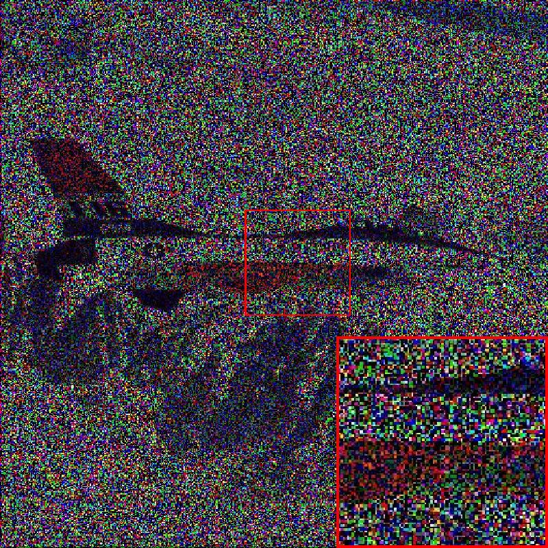
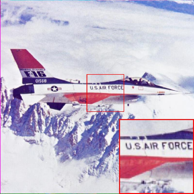
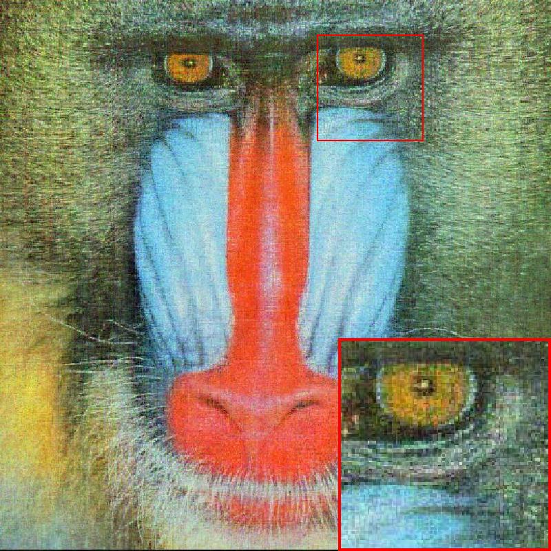
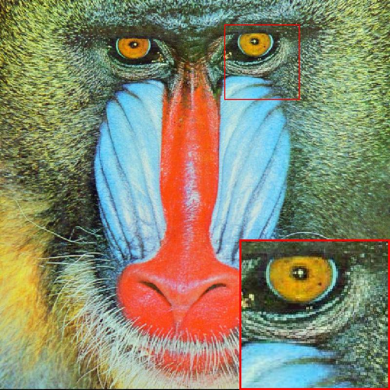
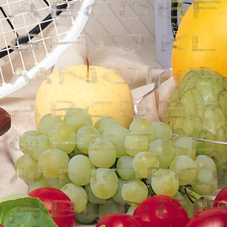
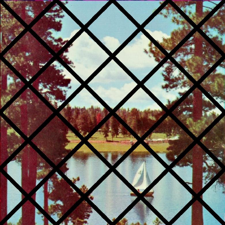
For visualization, we exhibit the recovered images with the sampling rate $30\%$ in Fig. 2. From the images illustrated in Fig. 2, we can find that the SNN-based method and TNN-based method are able to recover the general structure of the color images, while the details are unclear and results remain artifacts, which can be seen in the enlarged red boxes. The results by TNN-3DTV are relatively better. However, we can observe the over-smoothed phenomena in the enlarged areas. The recovered results by the proposed method are of high quality, being highly clear and very similar to the original images.

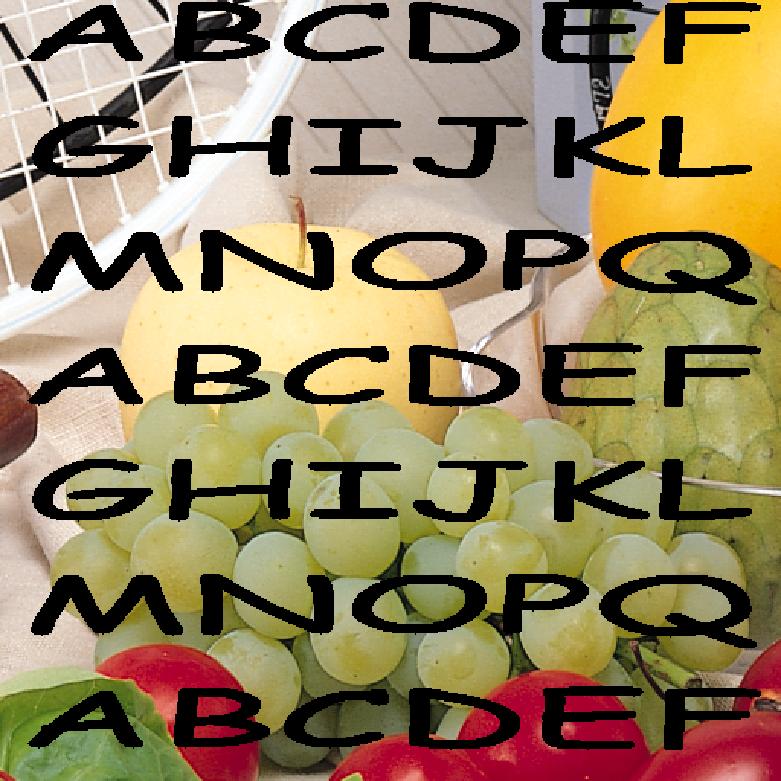
Now, we consider the structured samplings, i.e., inpainting and demosaicing, which are more difficult than the element-wise sampling. In image inpainting and demosaicing, we consider the tubal sampling (i.e., entries are sampled along all channels for a spatial location) and the Bayer pattern sampling (i.e., each two-by-two cell contains two green, one blue, and one red), respectively. In inpainting, there are three different kinds of masks: letters, graffiti, and grid, respectively. Fig. 3 shows the inpainting and demosaicing results by different methods on color images: Fruits, Lena, Sailboat, and Baboon. It is easy to observe that the proposed method is superior to competing methods in inpainting and demosaicing experiments.

Observed	SNN	TNN	TNN-3DTV	DP3LRTC	Ground truth
PSNR 13.17 dB	PSNR 26.58 dB	PSNR 27.24 dB	PSNR 28.68 dB	PSNR 34.57 dB	PSNR inf
PSNR 14.78 dB	PSNR 29.21 dB	PSNR 29.12 dB	PSNR 30.18 dB	PSNR 32.91 dB	PSNR inf
PSNR 12.18 dB	PSNR 26.03 dB	PSNR 25.83 dB	PSNR 26.99 dB	PSNR 28.47 dB	PSNR inf
PSNR 6.95 dB	PSNR 9.81 dB	PSNR 6.95 dB	PSNR 23.08 dB	PSNR 26.23 dB	PSNR inf

Figure 3: Inpainting (top three rows) and demosaicing (bottom row) results by SNN [18], TNN [28], TNN-3DTV [37], and the proposed method on color images.

4.2 Video Completion

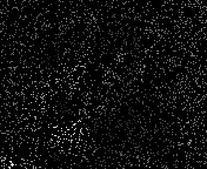
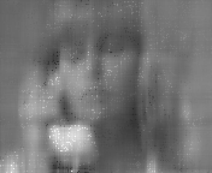
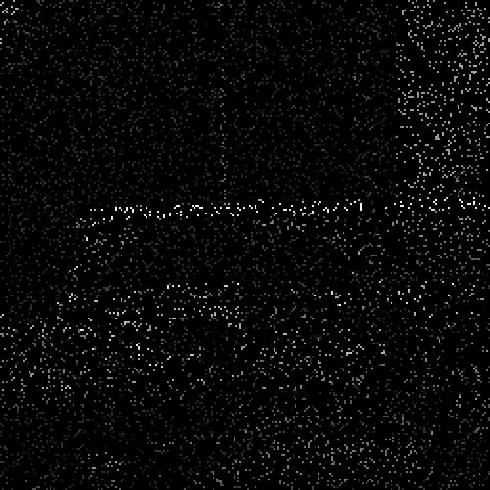
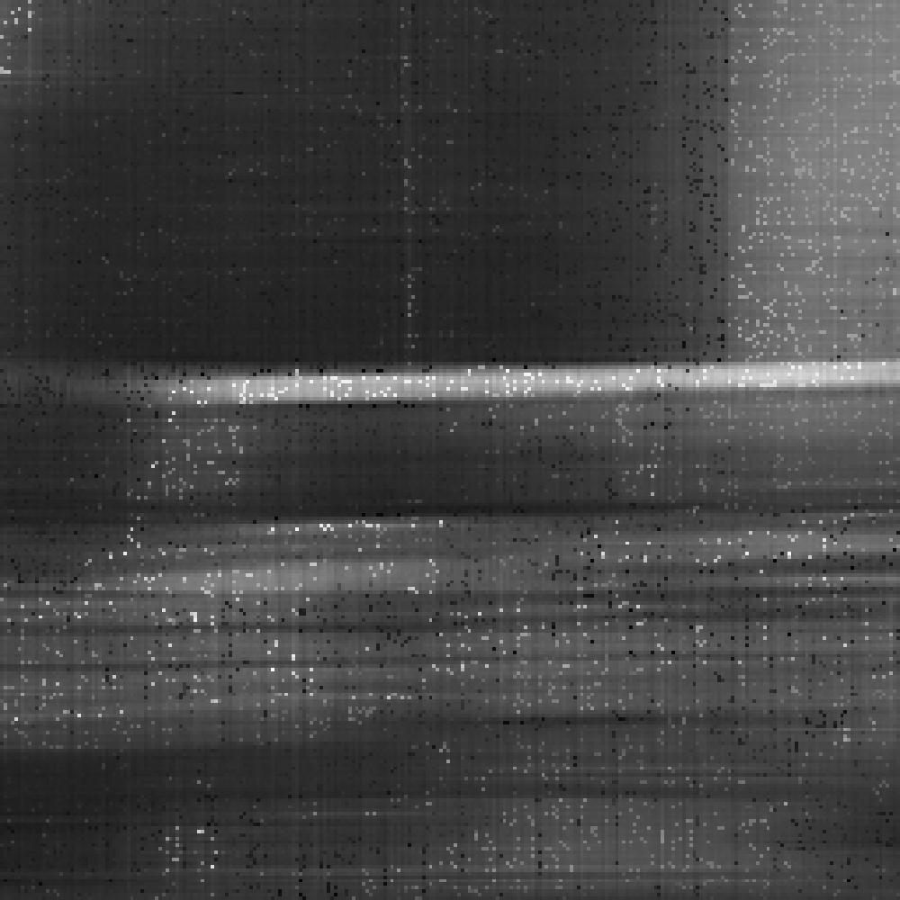
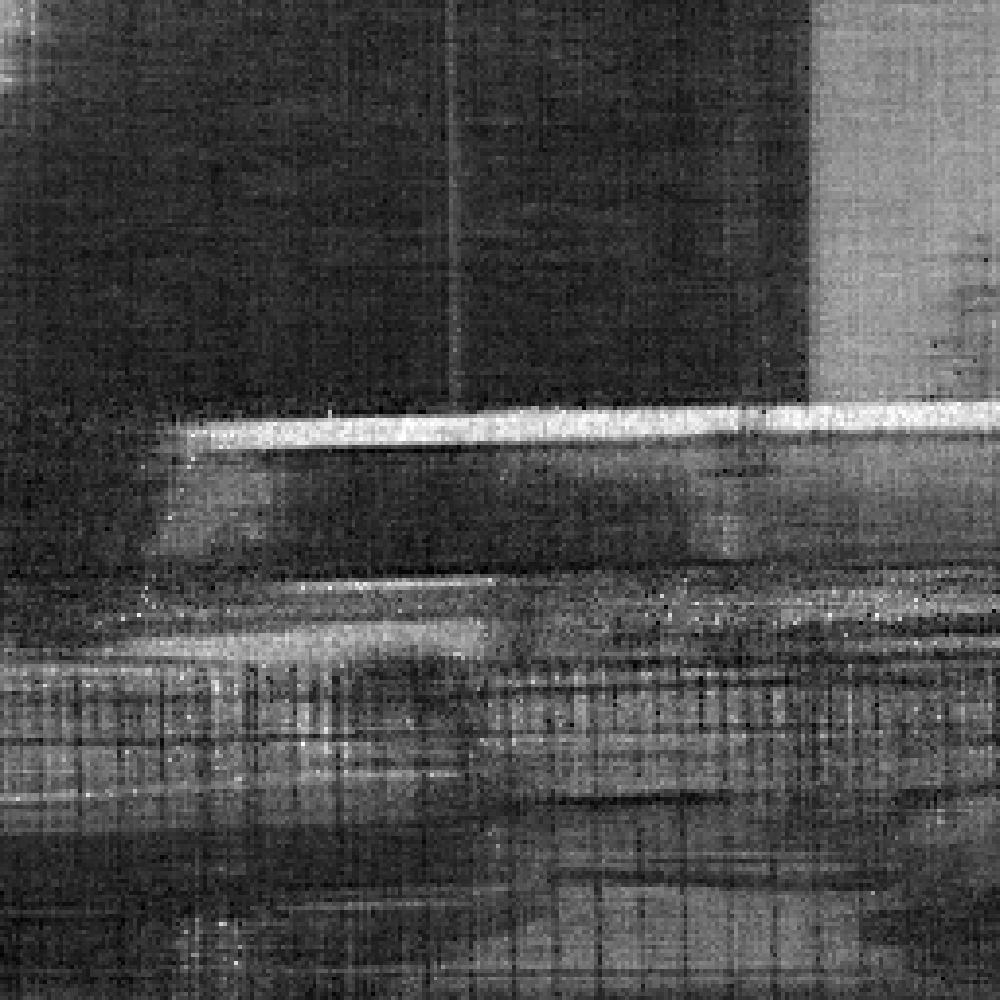
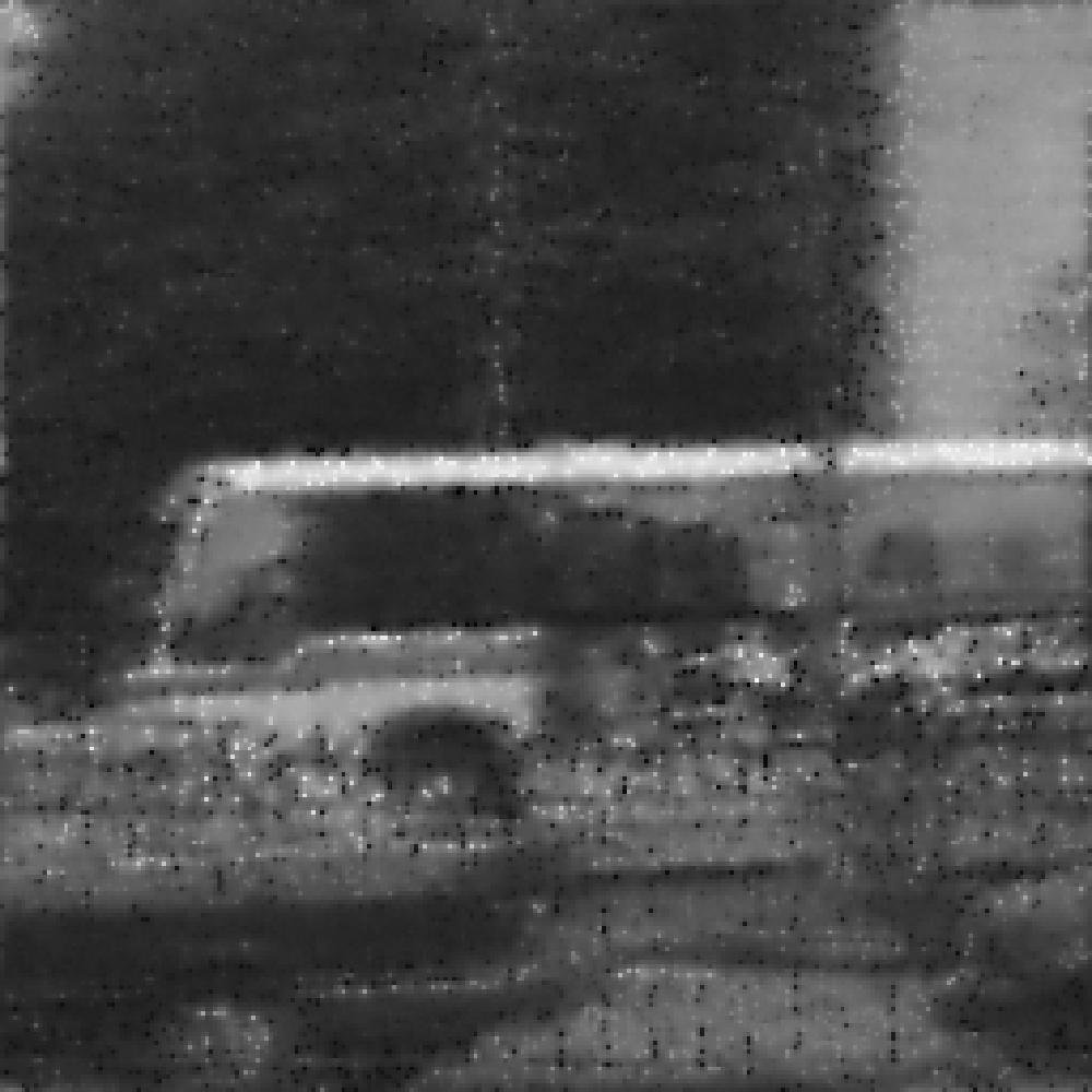
In this subsection, 5 grayscale videos with different sizes are selected. For gray videos, we feed the spatial slices into the FFDNet denoiser trained for gray images as the PnP denoiser. Tab. 2 lists the PSNR and SSIM values of the recovered video results by different methods with different sampling rates. It is easy to observe that DP3LRTC obtains the results with the highest performance evaluation indices. For visualization, we show the 20-th frame of the recovered videos with the sampling rate $20\%$ in Fig. 4. We can see that the results recovered by DP3LRTC are of higher quality than the results obtained by compared methods.

Table 2: Quantitative comparison of the results by SNN [18], TNN [28], TNN-3DTV [37], and the proposed method on videos. The best and second best values are highlighted in bold and underlined, respectively.

Video	SR	PSNR					SSIM					Time (s)
		SNN	TNN	TNN-3DTV	DP3LRTC		SNN	TNN	TNN-3DTV	DP3LRTC		SNN	TNN	TNN-3DTV	DP3LRTC
Akiyo $144\times 176\times 30$	5%	20.18	28.33	28.76	30.59		0.5976	0.8630	0.8949	0.9294		5	20	56	54
	10%	23.64	31.16	31.97	33.33		0.7340	0.9272	0.9452	0.9623		3	20	56	51
	20%	27.54	34.82	36.06	36.96		0.8642	0.9674	0.9777	0.9816		3	20	57	52
Suzie $144\times 176\times 30$	5%	20.84	26.37	27.39	29.37		0.5944	0.7203	0.7989	0.8373		4	19	56	51
	10%	24.40	28.41	29.27	31.80		0.7046	0.7976	0.8513	0.8899		3	18	56	51
	20%	28.12	31.14	31.95	34.75		0.8189	0.8739	0.9123	0.9358		2	18	57	52
Container $144\times 176\times 30$	5%	19.81	26.27	26.63	26.87		0.6446	0.8305	0.8611	0.8695		4	19	56	51
	10%	22.26	29.53	30.05	30.44		0.7413	0.9023	0.9272	0.9230		3	19	56	51
	20%	25.56	33.65	34.69	34.82		0.8495	0.9553	0.9677	0.9654		2	19	57	52
News $144\times 176\times 30$	5%	18.34	26.65	27.20	28.29		0.5610	0.8182	0.8738	0.9023		4	20	56	51
	10%	21.47	30.31	30.56	31.96		0.6955	0.9106	0.9285	0.9473		3	20	57	51
	20%	25.00	33.82	34.21	35.55		0.8256	0.9554	0.9665	0.9740		3	21	57	52
Bus $256\times 256\times 30$	5%	15.79	18.30	18.36	20.78		0.3300	0.3331	0.3973	0.5932		11	52	185	145
	10%	17.70	19.61	19.66	22.83		0.4174	0.4421	0.5083	0.7222		9	50	185	146
	20%	19.86	21.74	21.91	25.48		0.5560	0.5993	0.6778	0.8359		5	50	187	148
Average	5%	18.99	25.18	25.67	27.18		0.5455	0.7130	0.7652	0.8263		6	26	82	70
	10%	21.89	27.80	28.30	30.07		0.6586	0.7960	0.8321	0.8889		4	25	82	70
	20%	25.22	31.03	31.76	33.51		0.7828	0.8703	0.9004	0.9385		3	26	83	71

Observed	SNN	TNN	TNN-3DTV	DP3LRTC	Ground truth

Figure 4: The $20$-th frame of the videos recovered by SNN, TNN, TNN-3DTV, and DP3LRTC with the sampling rate $10\%$.

4.3 MSI Completion

In this subsection, we test 7 MSIs from the CAVE dataset which are of size $256\times 256\times 31$ with the wavelengths in the range of $400\sim 700$ nm at an interval of 10 nm. For MSIs, we feed the spatial slices into the FFDNet denoiser trained for gray images as the PnP denoiser.

Table 3: Quantitative comparison of the results by SNN [18], TNN [28], TNN-3DTV [37], and the proposed method on MSIs. The best and second best values are highlighted in bold and underlined, respectively.

MSI	SR	PSNR					SSIM					Time (s)
		SNN	TNN	TNN-3DTV	DP3LRTC		SNN	TNN	TNN-3DTV	DP3LRTC		SNN	TNN	TNN-3DTV	DP3LRTC
Balloons $256\times 256\times 31$	5%	24.29	31.35	32.66	39.04		0.8232	0.8670	0.9381	0.9843		8	58	191	144
	10%	31.27	35.63	37.66	42.98		0.9242	0.9380	0.9735	0.9937		7	61	200	155
	20%	37.34	41.11	42.77	47.54		0.9737	0.9803	0.9904	0.9975		7	59	192	147
Beads $256\times 256\times 31$	5%	16.50	19.86	21.27	22.53		0.3259	0.4569	0.6506	0.6912		9	60	199	147
	10%	17.99	22.92	23.95	26.08		0.4191	0.6512	0.7907	0.8369		7	61	198	153
	20%	21.34	27.61	27.78	30.20		0.6404	0.8420	0.9024	0.9319		7	58	197	152
Cd $256\times 256\times 31$	5%	22.19	26.51	29.35	30.22		0.8497	0.8029	0.9251	0.9597		10	62	191	144
	10%	25.98	29.54	31.92	35.30		0.9018	0.8871	0.9550	0.9790		10	69	196	157
	20%	30.85	33.22	36.04	39.35		0.9498	0.9447	0.9791	0.9890		8	64	193	150
Clay $256\times 256\times 31$	5%	28.83	33.62	34.25	39.89		0.9224	0.9052	0.9487	0.9680		10	59	194	145
	10%	35.78	38.22	39.66	43.80		0.9726	0.9657	0.9819	0.9907		9	62	193	144
	20%	41.58	43.69	44.69	48.02		0.9895	0.9813	0.9890	0.9952		9	62	191	147
Face $256\times 256\times 31$	5%	25.64	32.32	32.70	36.82		0.8346	0.8981	0.9381	0.9663		9	61	198	146
	10%	30.51	36.50	37.52	39.66		0.9125	0.9548	0.9736	0.9829		8	60	192	145
	20%	36.20	41.33	42.00	42.96		0.9664	0.9842	0.9778	0.9916		8	61	192	147
Feathers $256\times 256\times 31$	5%	20.45	27.55	28.23	31.14		0.6565	0.7694	0.8712	0.9375		7	58	196	151
	10%	24.58	31.19	31.83	34.59		0.7925	0.8717	0.9308	0.9656		8	58	193	147
	20%	29.30	35.86	36.73	38.68		0.8995	0.9481	0.9726	0.9838		8	60	193	150
Flowers $256\times 256\times 31$	5%	20.47	26.75	27.90	30.34		0.6293	0.7153	0.8288	0.8894		10	60	196	148
	10%	24.88	30.36	31.37	33.70		0.7605	0.8357	0.9025	0.9419		7	58	192	147
	20%	29.49	35.33	36.25	37.66		0.8804	0.9342	0.9621	0.9745		7	60	194	149
Average	5%	22.62	28.28	29.48	32.85		0.7202	0.7735	0.8715	0.9138		9	60	195	146
	10%	27.28	32.05	33.42	36.59		0.8119	0.8720	0.9297	0.9558		8	61	195	150
	20%	32.30	36.88	38.04	40.63		0.9000	0.9450	0.9676	0.9805		8	60	193	149

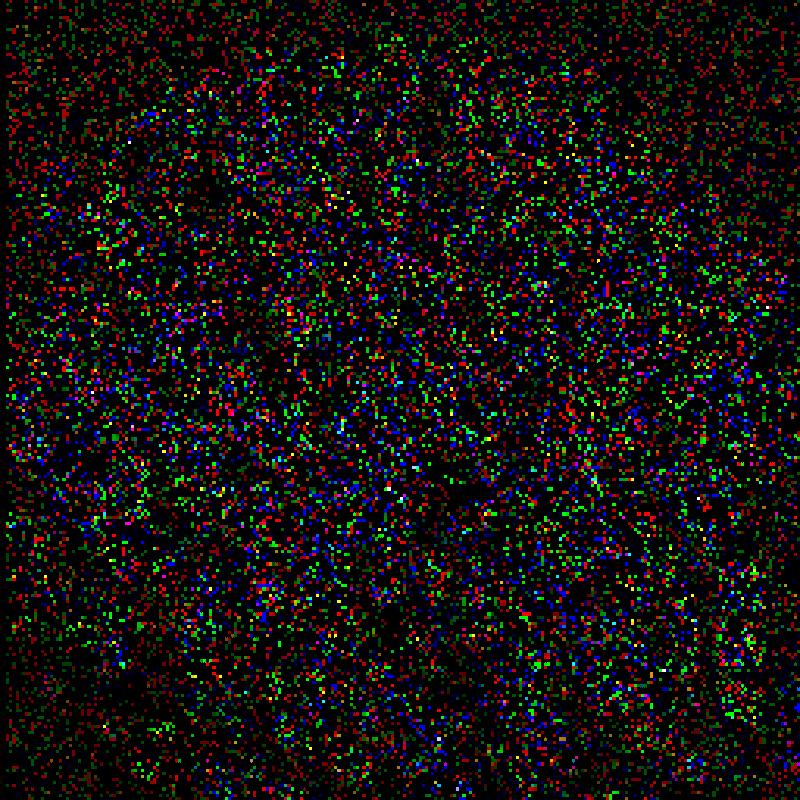
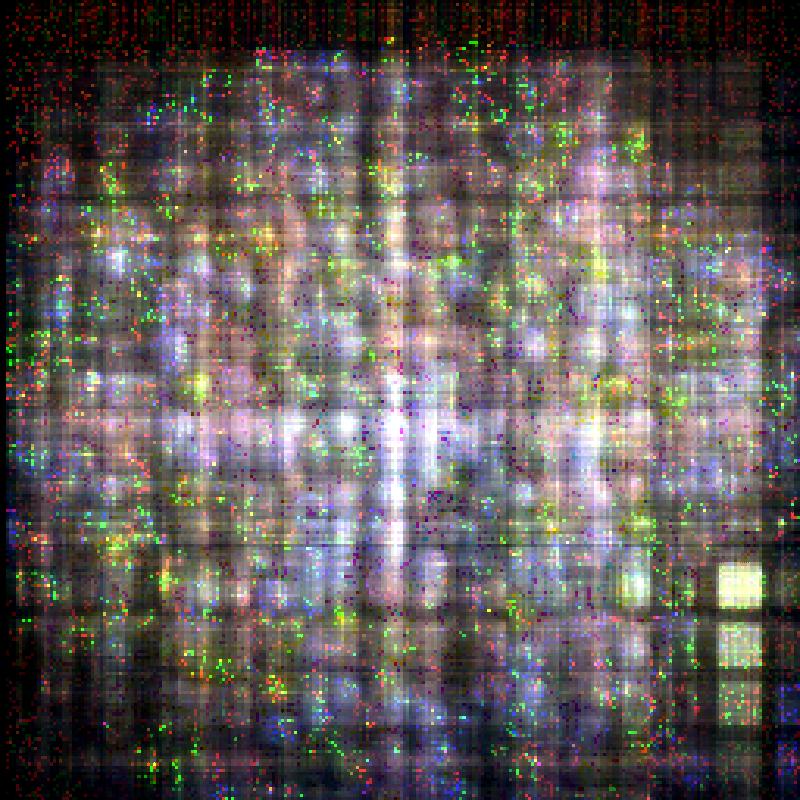
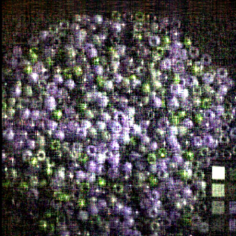
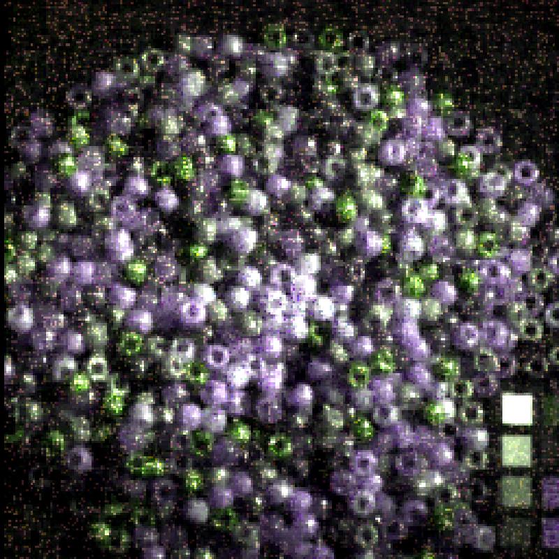
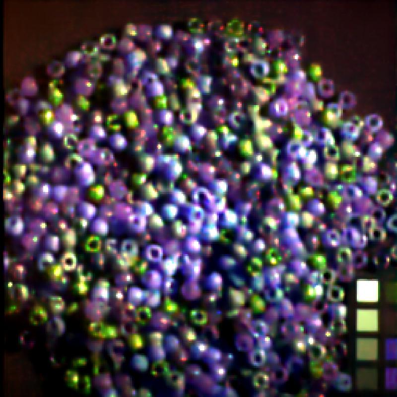
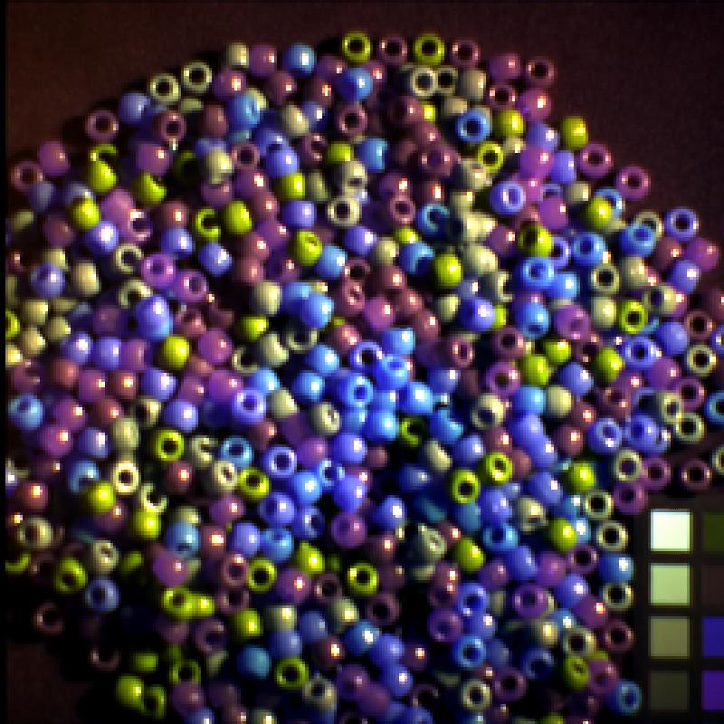
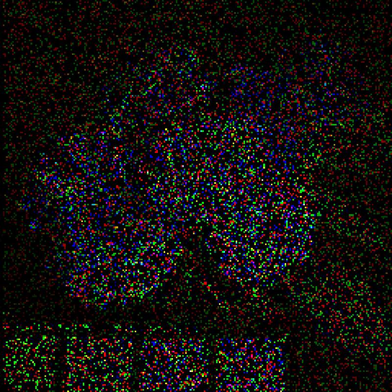
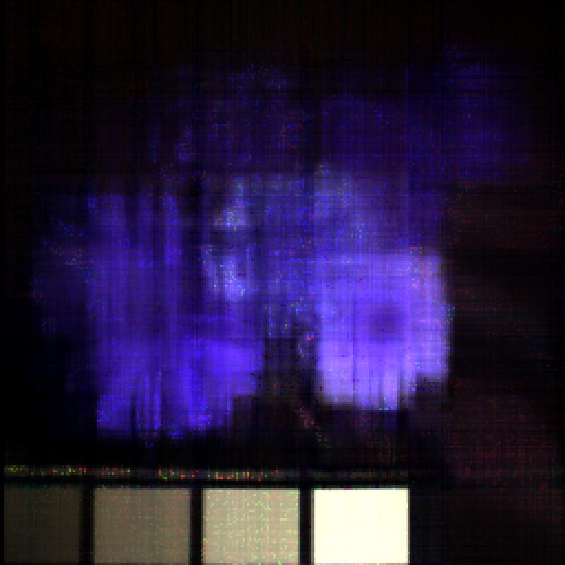
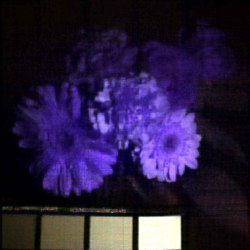
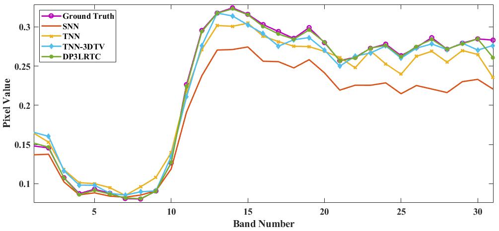
Tab. 4 exhibits the PSNR and SSIM values of all the results by different methods. The DP3LRTC achieves the highest PSNR and SSIM values, while the TNN-3DTV gets the second best. Fig. 5 displays the recovered MSIs (pseudo-color images composed of the 1st, 2nd, and 31-st bands) by different methods with the sampling rate $10\%$. From Fig. 5, it can be observed that the results recovered by DP3LRTC are of the highest quality. In Fig. 6, we display one selected tube of results recovered by SNN, TNN, TNN-3DTV, and DP3LRTC on MSI Balloons with the sampling rate 10%. We can observe that the selected tube of the MSI recovered by DP3LRTC is closer to the ground truth as compared with those by SNN, TNN, and TNN-3DTV.

Observed	SNN	TNN	TNN-3DTV	DP3LRTC	Ground truth

Figure 5: The MSIs (pseudo-color images composed of the 1st, 2nd, and 31-st bands) recovered by SNN, TNN, TNN-3DTV, and DP3LRTC with the sampling rate $10\%$.

Figure 6: The selected tubes of results recovered by by SNN [18], TNN [28], TNN-3DTV [37], and the proposed method on the MSI Balloons with the sampling rate 10%.

4.4 Discussions

4.4.1 Convergence Behaviour

The numerical experiments have shown the great empirical success of DP3LRTC. However, it is still an open question whether the ADMM algorithm under the PnP framework has a good convergence behavior. In Fig. 7, we displayed the relative change curves of the ADMM algorithm (in the logarithmic scale) with respect to the iteration on different videos. We can evidently observe the numerical convergence of the ADMM algorithm.

Figure 7: The convergence curves of the ADMM algorithm on videos Akiyo, Suzie, Container, News, and Bus with the sampling rate $10\%$.

4.4.2 Contributions of Different Terms

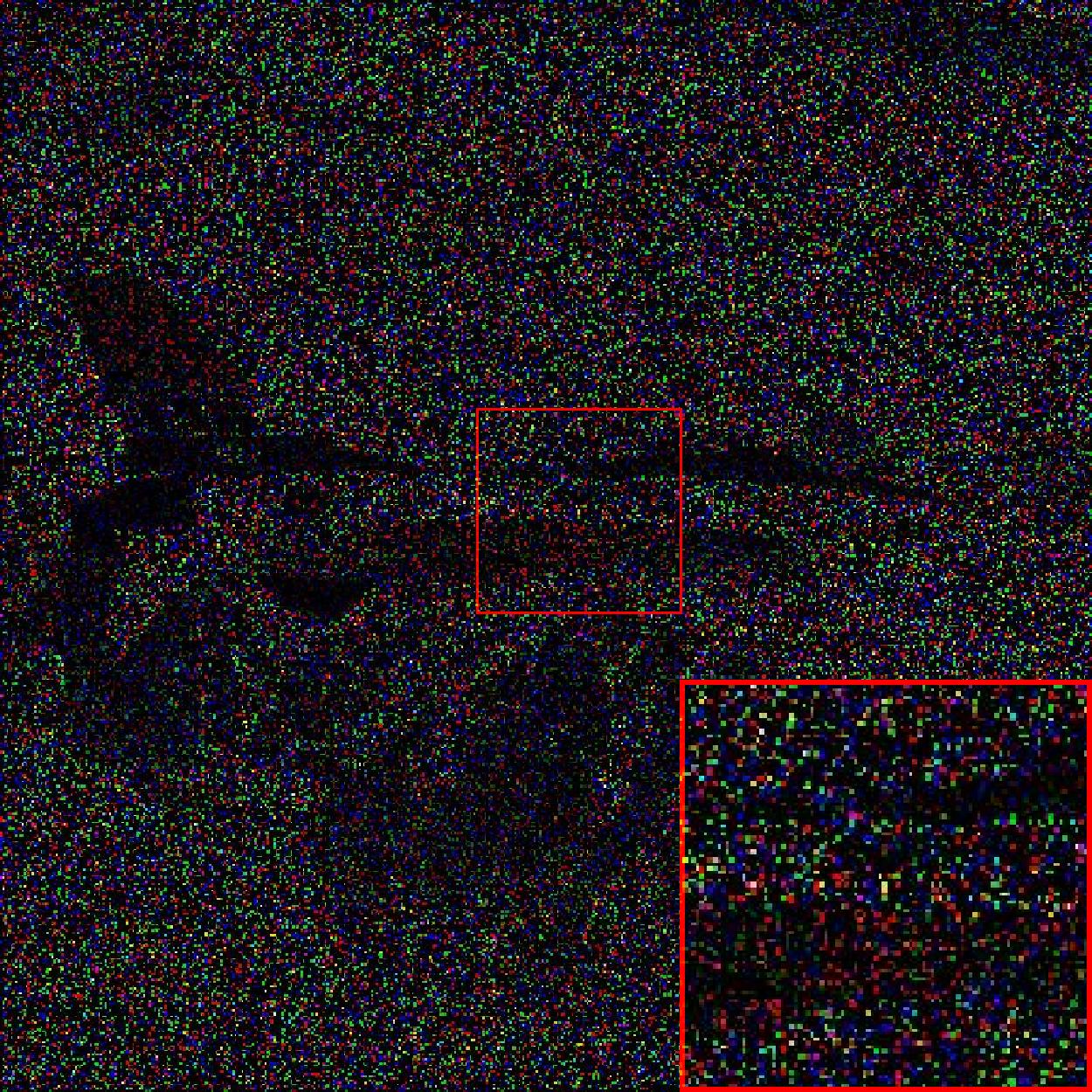
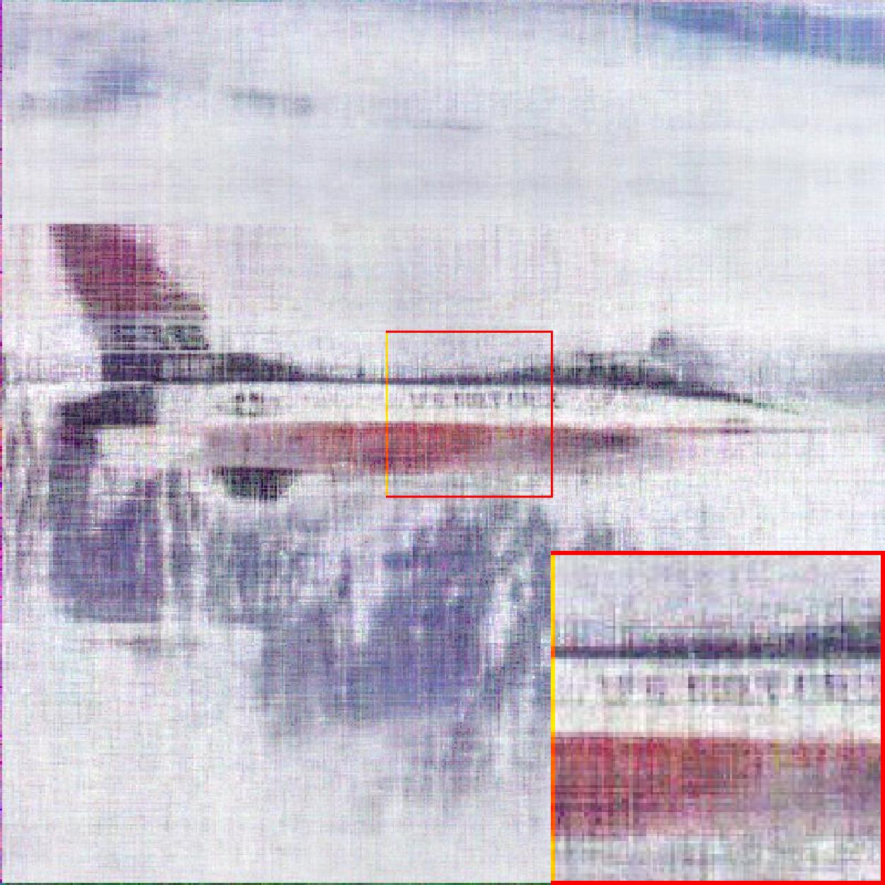
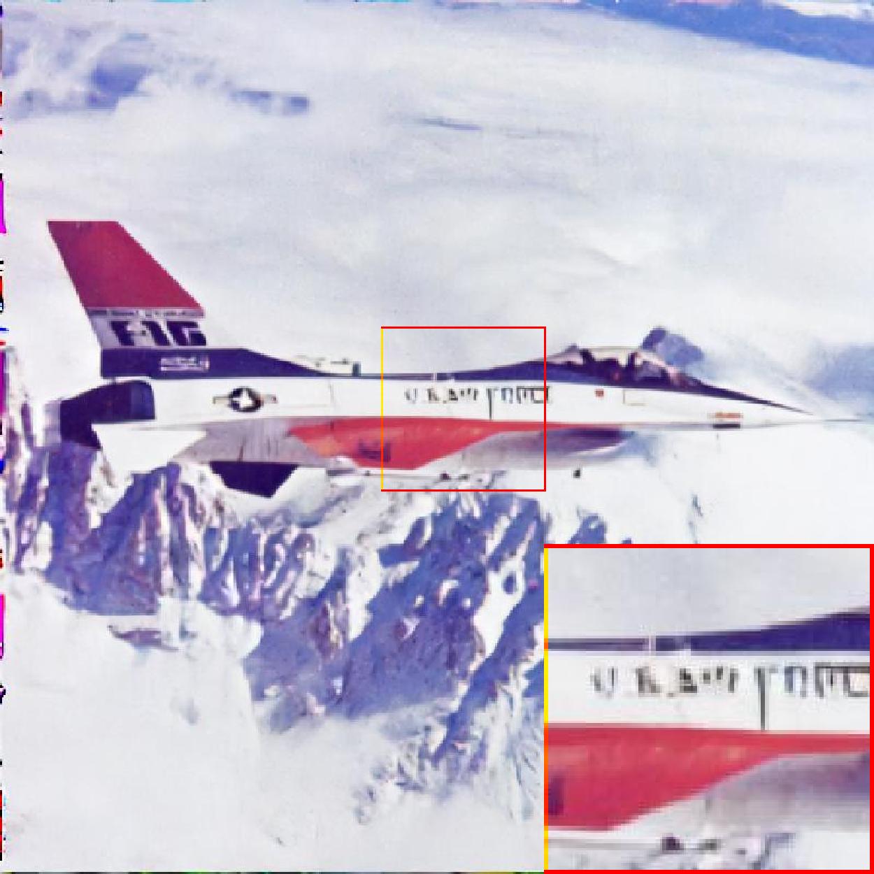
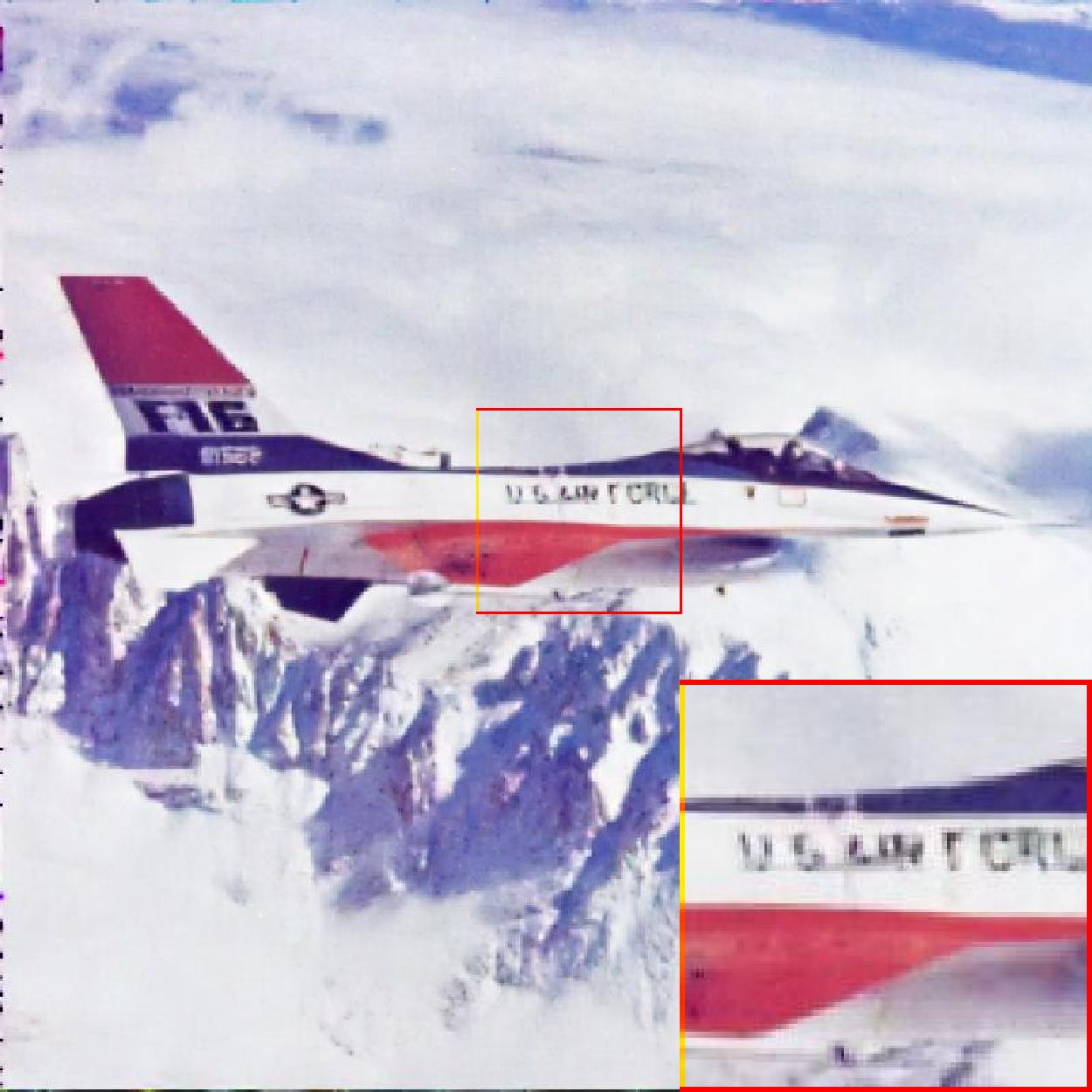
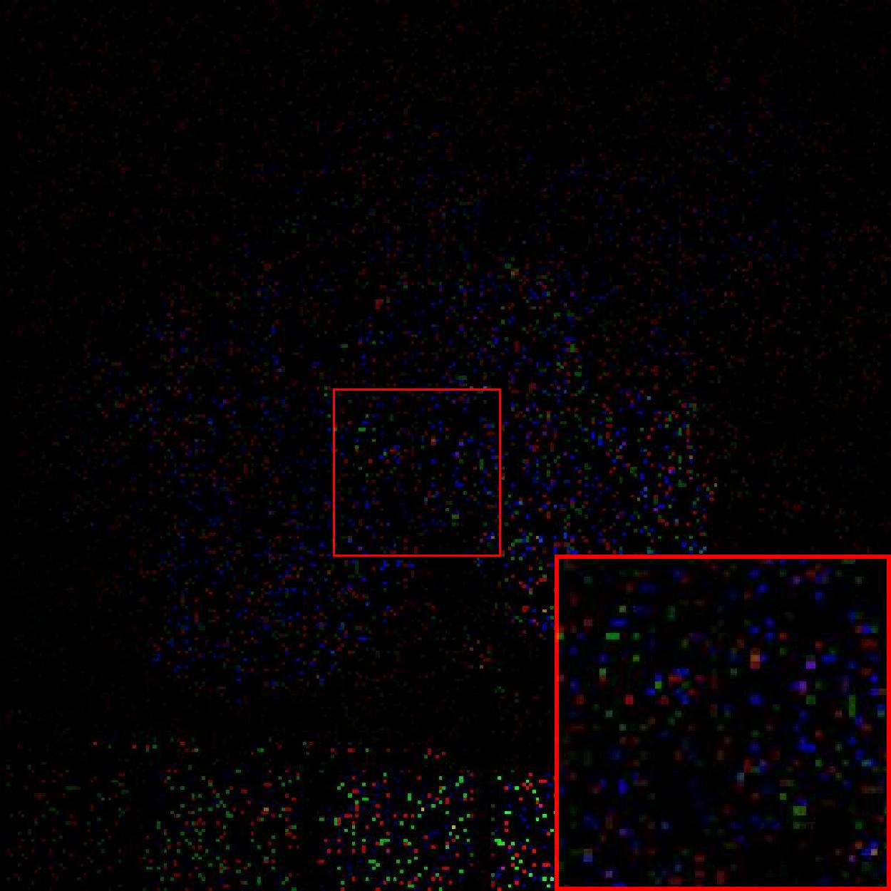
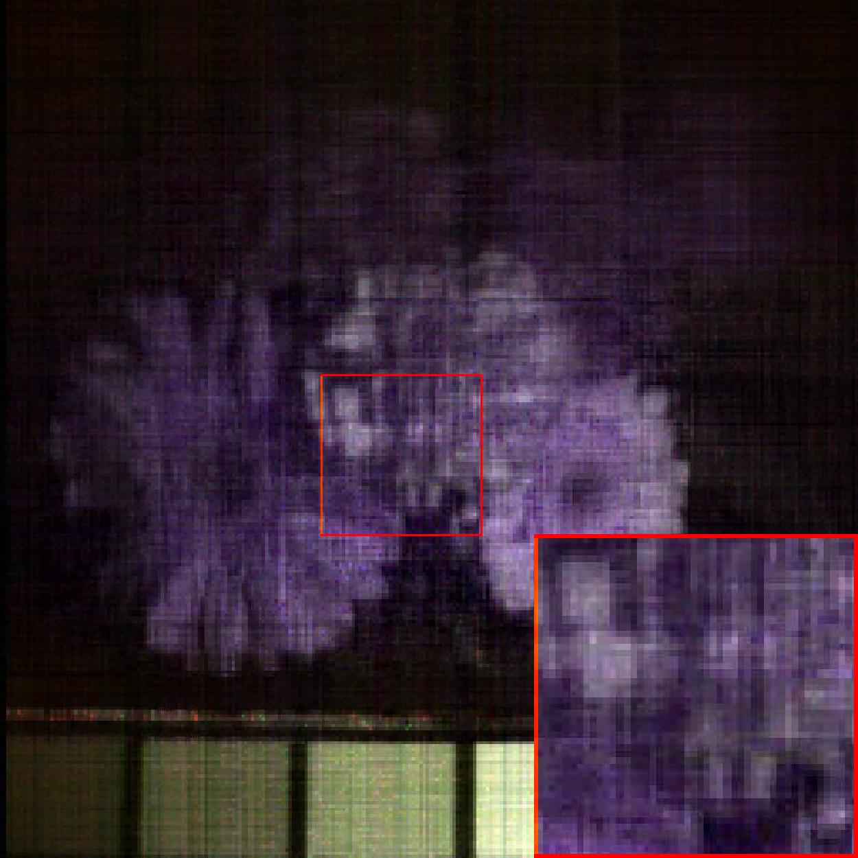
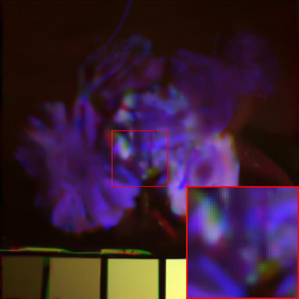
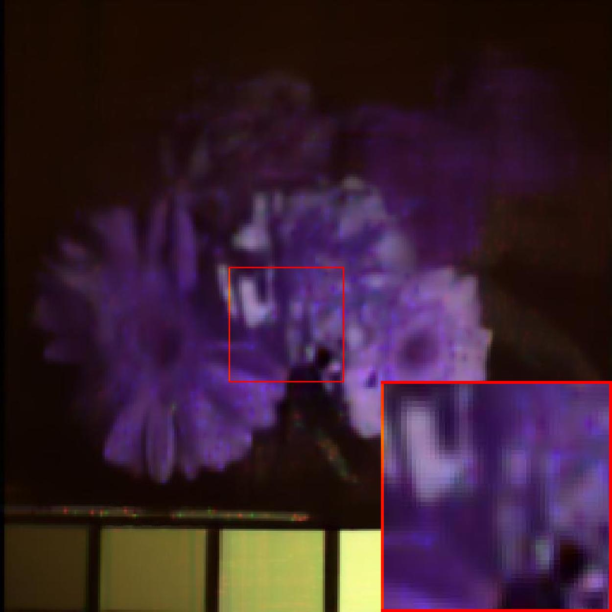
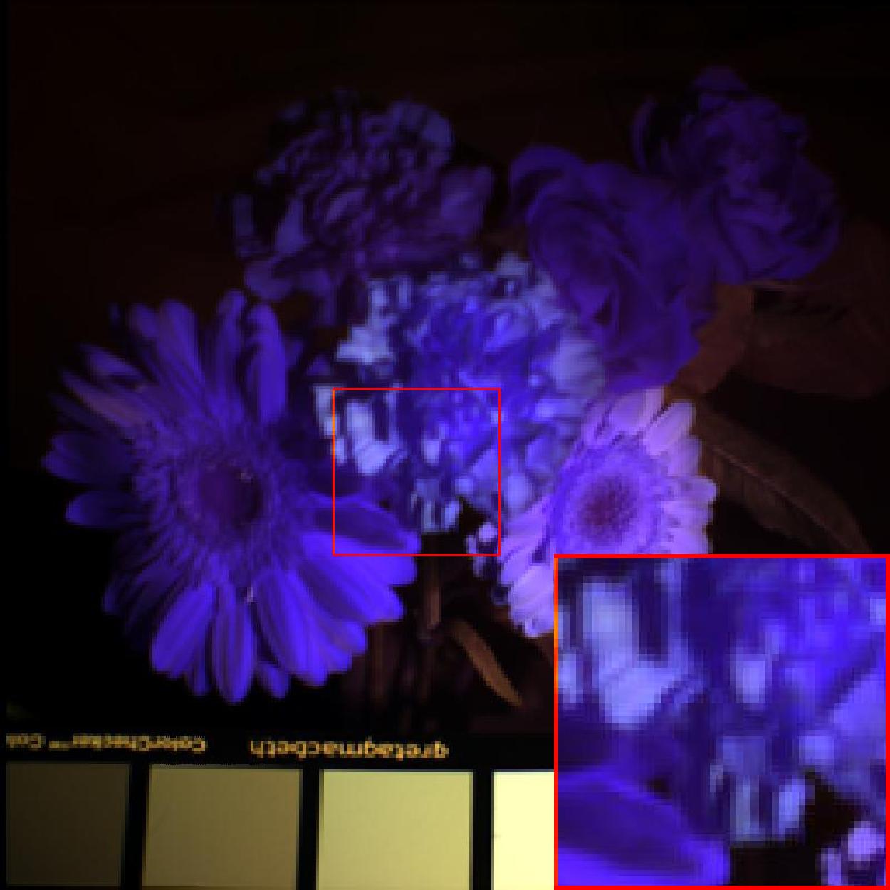
To evaluate the distinct contributions of the low-rankness prior and deep image prior, we test the performance of 3 methods: TNN (only the TNN regularizer), DPR (only the implicit deep regularizer), and DP3LRTC (both the TNN and implicit deep regularizers). In Fig. 8, we exhibit the recovered results by TNN, DPR, and DP3LRTC on color image Airplane and MSI Flowers, together with PSNR values. In Fig. 8, the results by DPR are clearer than those by TNN. This shows the remarkable ability of CNN denoiser to capture the spatial structures. Meanwhile, we can observe that the performance of DPR is comparable to DP3LRTC on color images, since that color images only consists of 3 color channels. However, from the enlarged areas, we can see obvious artifact in the result by DPR. When reconstructing the MSI, which consists of 31 spectral bands, TNN and DP3LRTC outperform DPR. This shows that the TNN regularizer is good at utilizing the spectral redundancy. Therefore, we can confirm that two regularizers are indispensable to DP3LRTC and benefit from each other. Together, they contribute to the superior performance of the proposed DP3LRTC.

Observed	TNN	DPR	DP3LRTC	Ground truth
PSNR 2.27 dB	PSNR 21.94 dB	PSNR 26.29 dB	PSNR 28.48 dB	PSNR inf
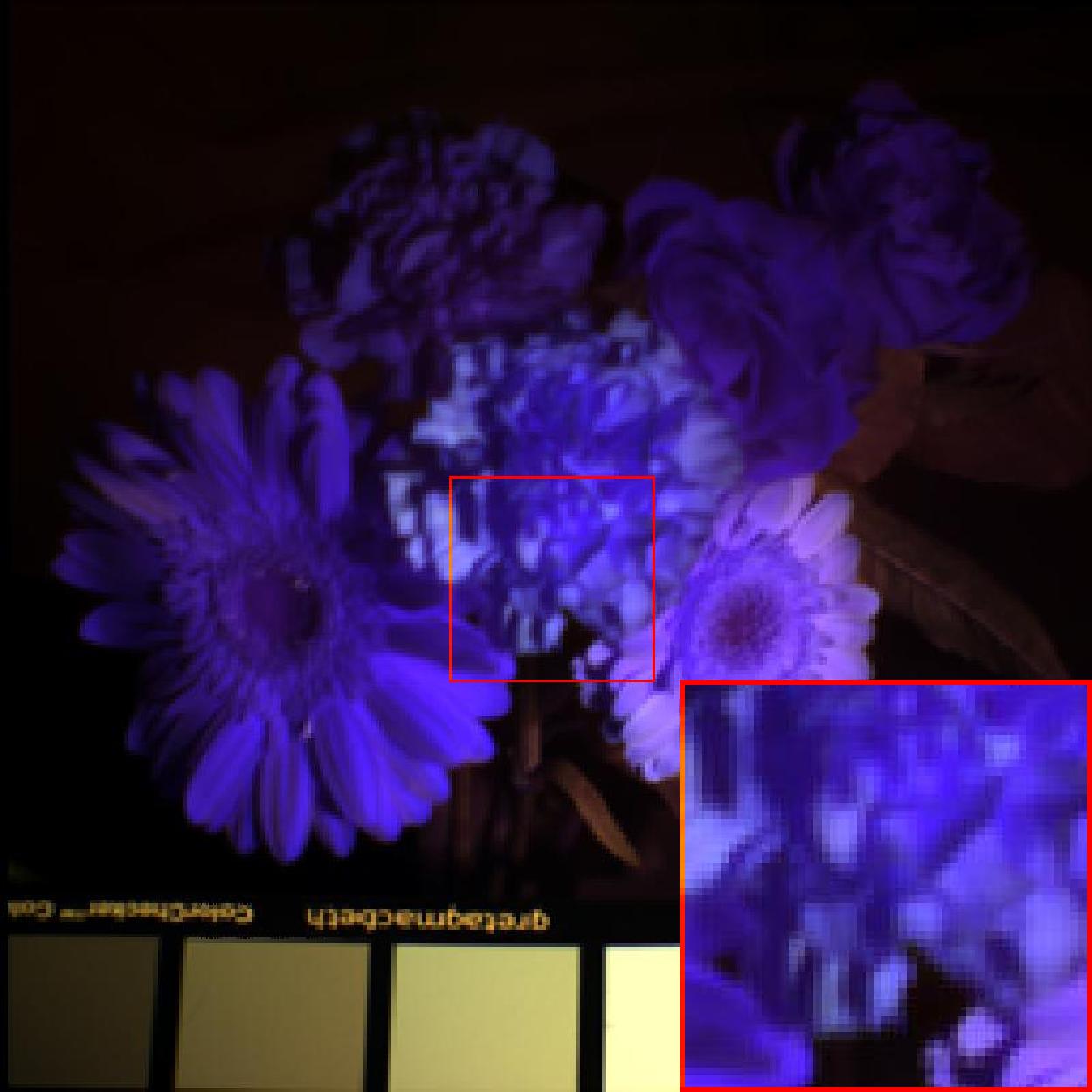PSNR 14.05 dB	PSNR 26.75 dB	PSNR 24.08 dB	PSNR 30.34 dB	PSNR inf

Figure 8: First row: the recovered results by TNN, DPR, and DP3LRTC on color image Airplane with the sampling rate 10%. Second row: the recovered results (pseudo-color images composed of the 1st, 2nd, and 31-th bands) by TNN, DPR, and DP3LRTC on MSI Flowers with the sampling rate 5%.

To take a little more in-depth look at the mechanism of each term, we conduct experiments on all 8 MSIs in Sec. 4.3 with different sampling rates. The averaged PSNR and SSIM values are reported in Tab. 4. Generally, the metric SSIM evaluates the local structure similarity [57] and the metric PSNR reflects the overall recovery quality. The PSNR values of results by TNN are higher than those by DPR, while DPR achieves higher SSIM values. This phenomenon also reveals that the TNN regularizer is more suitable for characterising the global information and the CNN denoiser is appropriate for recovering the fine structures. As the sampling rate increases, the SSIM margin between TNN and DP3LRTC decreases from 0.140 to 0.036 while the PSNR margin is always around 4dB. This shows that in the low sampling cases, recovering the local structure becomes more difficult than capturing the global information.

Table 4: Quantitative comparison of the results by different methods on MSIs. The best are highlighted in bold.

MSI	SR	PSNR			SSIM
		TNN	DPR	DP3LRTC	TNN	DPR	DP3LRTC
Average	5%	28.28	24.80	32.85	0.7735	0.8631	0.9138
	10%	32.05	30.64	36.59	0.8720	0.9111	0.9558
	20%	36.88	36.24	40.63	0.9443	0.9516	0.9805

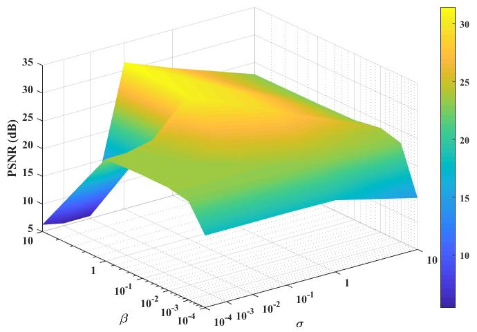
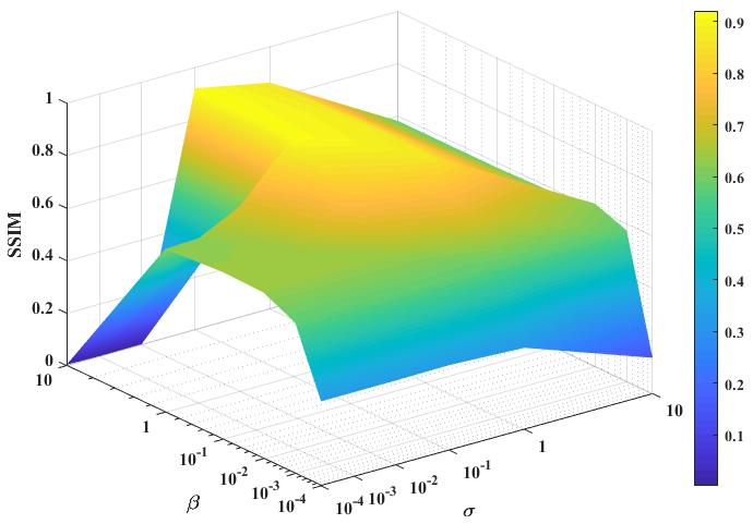
Moreover, we study the influence of parameters $\beta$ and $\sigma$. In Fig. 9, we show the PSNR and SSIM values of the results recovered by DP3LRTC on color image Starfish with respect to $\beta$ and $\sigma$. We can see that DP3LRTC delivers the best performance when $\beta\in\{10^{-1},1\}$ and $\sigma\in\{10^{-2},10^{-1},1\}$.

Figure 9: The PSNR and SSIM values of the results recovered by DP3LRTC with respect to $\beta$ and $\sigma$ on color image Starfish with the sampling rate $20\%$.

4.4.3 Low-matrix-rank and Low-tensor-rank

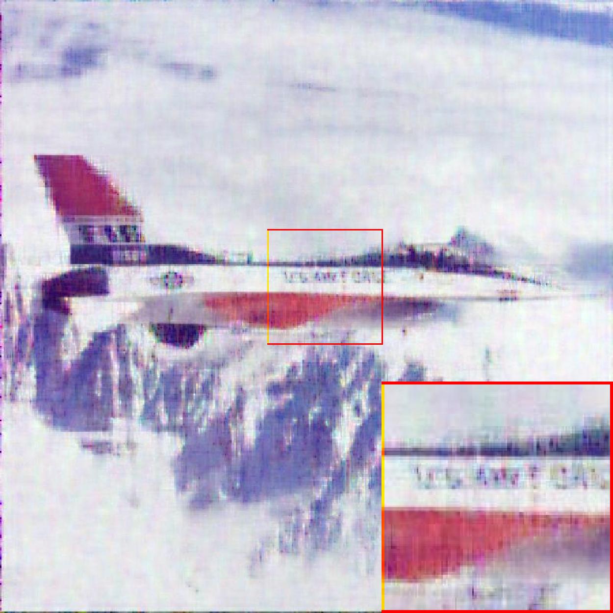
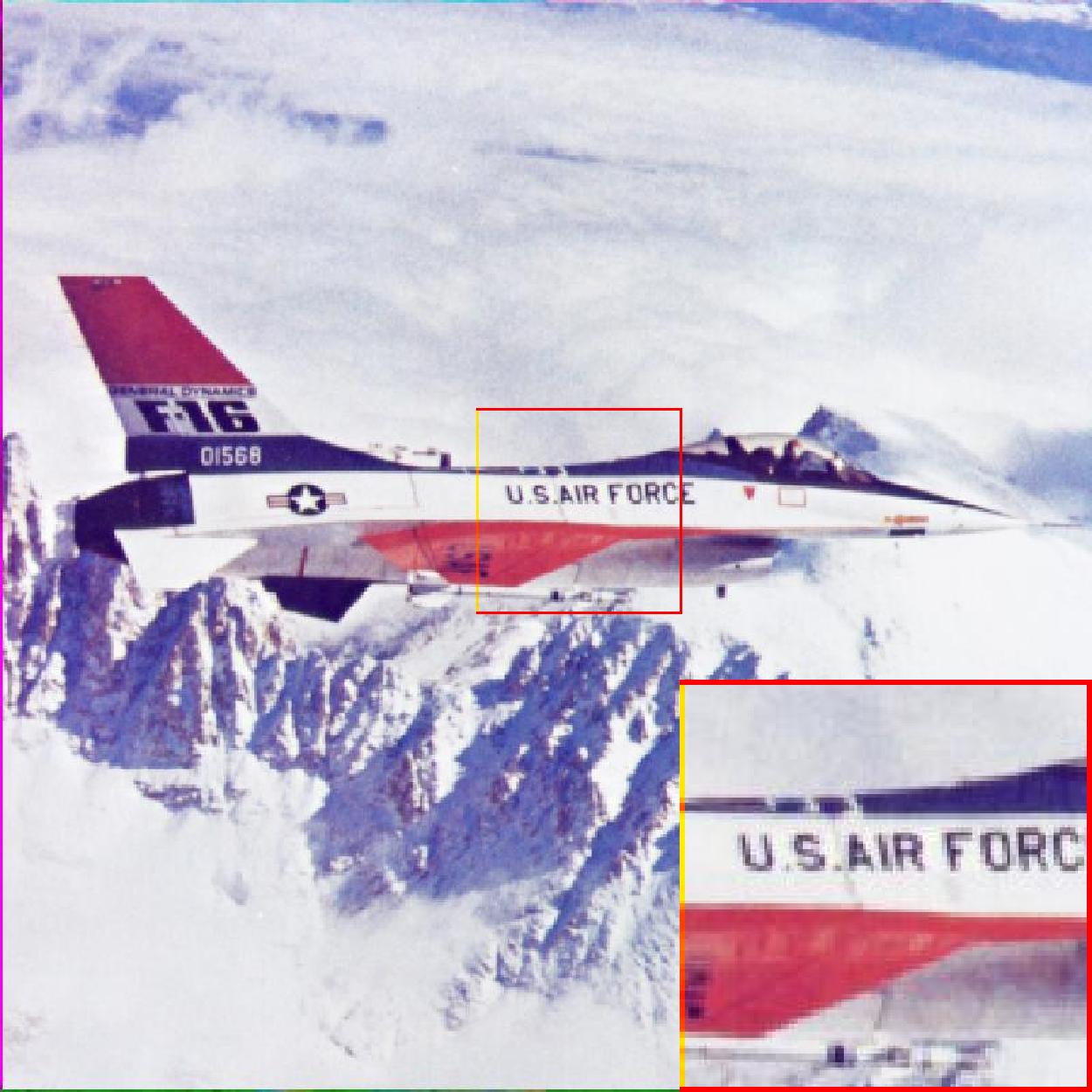
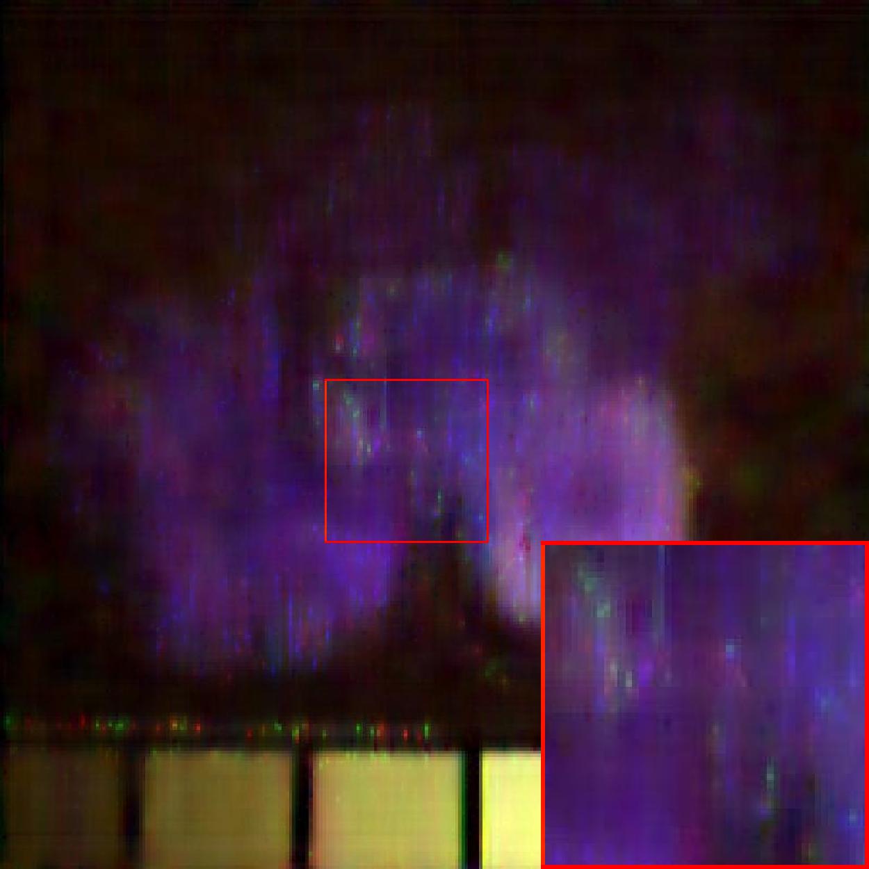
To illustrate the superiority of the tensor-rank-based model, we reported the quantitative comparison of the recovered results by our DP3LRTC and DP3LRMC, in which the TNN is replaced by the matrix nuclear norm of the matricization of multi-dimensional images (where the rows represent the vectorized spatial images and the columns the spectral channels), on color images and multi-spectral images (MSIs) in Tabs. 5. The setup of experiments on color images and the multispectral images are the same as Sec. 4.1 and Sec. 4.3, respectively. Similarly, we only report the average indexes of the results. For better visual inspection, we further displayed the recovered results by DP3LRMC and DP3LRTC in Fig. 10. From Tab. 5 and Fig. 10, we confirmed that the tensor-rank-based model DP3LRTC is evidently better than the matrix-rank-based model DP3LRMC.

Table 5: Quantitative comparison of the results by different methods on color images. The best are highlighted in bold.

	SR	PSNR		SSIM
		DP3LRMC	DP3LRTC	DP3LRMC	DP3LRTC
Color images (average)	10%	23.89	28.83	0.7630	0.9061
	20%	26.76	31.70	0.8719	0.9415
	30%	29.07	33.40	0.9308	0.9668
MSIs (average)	5%	25.76	32.85	0.6948	0.9138
	10%	28.75	36.59	0.7863	0.9558
	20%	32.27	40.63	0.8706	0.9805

Observed	DP3LRMC	DP3LRTC	Ground truth
PSNR 2.27 dB	PSNR 24.24 dB	PSNR 28.48 dB	PSNR inf
PSNR 14.05 dB	PSNR 24.54 dB	PSNR 30.34 dB	PSNR inf

Figure 10: First row: the recovered results by DP3LRMC and DP3LRTC on color image Airplane with the sampling rate 10%. Second row: the recovered results (pseudo-color images composed of the 1st, 2nd, and 31-th bands) by DP3LRMC and DP3LRTC on MSI Flowers with the sampling rate 5%.

4.4.4 Beyond TNN, FFDNet, and Third-order Tensors

Actually, in this work, we suggested a user-friendly LRTC framework which integrates low-rankness prior and the denoising prior. Tab. 6 shows the quantitative comparison of the results obtained by different combinations of low-rankness metrics and denoisers. The setup is the same as the color image completion with random missing pixels in Sec. 4.1. For saving space, we only report the average indexes of the results of 8 color images. In Tab. 6, “SNN-DPR” denotes the combination of the sum of the nuclear norm (SNN) and the FFDNet denoiser, while “TNN-BM3D” indicates that the tensor nuclear norm (TNN) is combined with the BM3D denoiser [49]. From Tab. 6, we can observe that the combination of the tensor nuclear norm and the FFDNet denoiser is best among all combinations. Thus, we choose the the combination of the tensor nuclear norm and the FFDNet denoiser as the representative example of DP3LRTC framework.

Table 6: Quantitative comparison of the recovered results by different methods on color images. The best are highlighted in bold.

Color image	SR	PSNR			SSIM
		SNN-DPR	TNN-BM3D	DP3LRTC	SNN-DPR	TNN-BM3D	DP3LRTC
Average	10%	28.55	27.80	28.83	0.9013	0.8754	0.9061 [t]
	20%	31.24	30.91	31.70	0.9461	0.9382	0.9415
	30%	32.59	33.25	33.40	0.9597	0.9641	0.9668

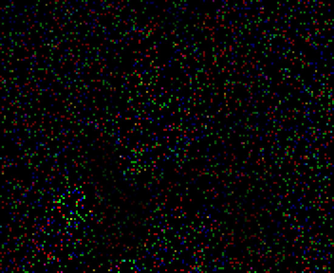
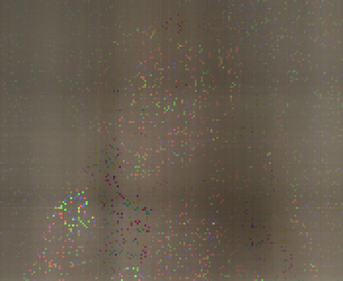
Next, we extend our DP3LRTC framework to high-order tensors ($n\geq 3$) by replacing the TNN regularizer with its high-order extension, i.e., the WSTNN in [27]. We conduct the experiment on a fourth-order tensor, the color video “Suzie” of size $144\times 176\times 3\times 100$. For color videos, we use the FFDNet network trained on color images as the PnP denoiser. When solving the $\mathcal{Z}$ subproblem in (16), we feed each frame of size $144\times 176\times 3$ into the CNN denoiser in sequence. The quantitative comparison of the recovered results by SNN, WSTNN, and DP3LRTC on color video Suzie is reported in Tab. 7. For better visual inspection, we further displayed the recovered results by SNN, WSTNN, and DP3LRTC in Fig. 11. We can observe that DP3LRTC can be extended to handle high-order tensors with the help of WSTNN. Also, we can generalize our method for high-order tensor via other low-rankness metrics, such as the “SNN-DPR”, and obtain remarkable performances.

Table 7: Quantitative comparison of the results by different methods on color video. The best are highlighted in bold.

Color Video	SR	PSNR			SSIM
		SNN	WSTNN	DP3LRTC	SNN	WSTNN	DP3LRTC
Suzie	1%	7.44	23.26	24.96	0.0372	0.6967	0.7371
	5%	17.97	28.24	30.73	0.5148	0.8384	0.8891
	10%	21.22	30.94	33.47	0.6139	0.8943	0.9285

Observed	SNN	TNN	DP3LRTC	Ground truth

Figure 11: The 50-th frame of the recovered color video Suzie by SNN, TNN, and DP3LRTC with the sampling rate 5%.

5 Conclusions

In this paper, we proposed a hybrid tensor completion model, in which the TNN regularizer is utilized to catch the global information and a data-driven implicit regularizer is used to express the local information. The proposed model simultaneously combines the model-based optimization method with the CNN-based method, in consideration of the global structure and fine detail preservation. An efficient ADMM is developed to solve the proposed model. Numerical experiments on different types of multi-dimensional images illustrate the superiority of the proposed method on the tensor completion problem.

References

- [1] L. Zhuang, J. M. Bioucas-Dias, Fast hyperspectral image denoising and inpainting based on low-rank and sparse representations, IEEE Journal of Selected Topics in Applied Earth Observations and Remote Sensing 11 (3) (2018) 730–742.
- [2] Y. Wang, J. Peng, Q. Zhao, Y. Leung, X.-L. Zhao, D. Meng, Hyperspectral image restoration via total variation regularized low-rank tensor decomposition, IEEE Journal of Selected Topics in Applied Earth Observations and Remote Sensing 11 (4) (2018) 1227–1243.
- [3] Y. Chang, L. Yan, H. Fang, C. Luo, Anisotropic spectral-spatial total variation model for multispectral remote sensing image destriping, IEEE Transactions on Image Processing 24 (6) (2015) 1852–1866.
- [4] J.-H. Yang, X.-L. Zhao, T.-H. Ma, Y. Chen, T.-Z. Huang, M. Ding, Remote sensing images destriping using unidirectional hybrid total variation and nonconvex low-rank regularization, Journal of Computational and Applied Mathematics 363 (2020) 124–144.
- [5] Q. Zhao, D. Meng, X. Kong, Q. Xie, W. Cao, Y. Wang, Z. Xu, A novel sparsity measure for tensor recovery, in: Proceedings of the IEEE International Conference on Computer Vision, 2015, pp. 271–279.
- [6] X. Luo, M. Zhou, S. Li, Z. You, Y. Xia, Q. Zhu, A nonnegative latent factor model for large-scale sparse matrices in recommender systems via alternating direction method, IEEE transactions on neural networks and learning systems 27 (3) (2015) 579–592.
- [7] X. Luo, M. Zhou, S. Li, L. Hu, M. Shang, Non-negativity constrained missing data estimation for high-dimensional and sparse matrices from industrial applications, IEEE transactions on cybernetics.
- [8] S. Li, M. Zhou, X. Luo, Modified primal-dual neural networks for motion control of redundant manipulators with dynamic rejection of harmonic noises, IEEE transactions on neural networks and learning systems 29 (10) (2017) 4791–4801.
- [9] L. Zhuang, J. M. Bioucas-Dias, Hy-Demosaicing: Hyperspectral blind reconstruction from spectral subsampling, in: Proceedings of the IEEE International Geoscience and Remote Sensing Symposium, 2018, pp. 4015–4018.
- [10] T. G. Kolda, B. W. Bader, Tensor decompositions and applications, SIAM Review 51 (3) (2009) 455–500.
- [11] Y. Wang, D. Meng, M. Yuan, Sparse recovery: from vectors to tensors, National Science Review 5 (5) (2017) 756–767.
- [12] Z. Long, Y. Liu, L. Chen, C. Zhu, Low rank tensor completion for multiway visual data, Signal Processing 155 (2019) 301–316.
- [13] N. D. Sidiropoulos, L. De Lathauwer, X. Fu, K. Huang, E. E. Papalexakis, C. Faloutsos, Tensor decomposition for signal processing and machine learning, IEEE Transactions on Signal Processing 65 (13) (2017) 3551–3582.
- [14] M. Che, A. Cichocki, Y. Wei, Neural networks for computing best rank-one approximations of tensors and its applications, Neurocomputing 267 (2017) 114–133.
- [15] X. Wang, M. Che, Y. Wei, Neural networks based approach solving multi-linear systems with m-tensors, Neurocomputing 351 (2019) 33–42.
- [16] Q. Zhao, L. Zhang, A. Cichocki, Bayesian CP factorization of incomplete tensors with automatic rank determination, IEEE Transactions on Pattern Analysis and Machine Intelligence 37 (9) (2015) 1751–1763.
- [17] C. J. Hillar, L.-H. Lim, Most tensor problems are NP-hard, Journal of the ACM 60 (6) (2013) 1–39.
- [18] J. Liu, P. Musialski, P. Wonka, J. Ye, Tensor completion for estimating missing values in visual data, IEEE Transactions on Pattern Analysis and Machine Intelligence 35 (1) (2013) 208–220.
- [19] S. Gandy, B. Recht, I. Yamada, Tensor completion and low-n-rank tensor recovery via convex optimization, Inverse Problems 27 (2) (2011) 025010.
- [20] Q. Xie, Q. Zhao, D. Meng, Z. Xu, Kronecker-basis-representation based tensor sparsity and its applications to tensor recovery, IEEE Transactions on Pattern Analysis and Machine Intelligence 40 (8) (2018) 1888–1902.
- [21] H. Tan, B. Cheng, J. Feng, G. Feng, W. Wang, Y.-J. Zhang, Low-n-rank tensor recovery based on multi-linear augmented lagrange multiplier method, Neurocomputing 119 (2013) 144–152.
- [22] T.-Y. Ji, T.-Z. Huang, X.-L. Zhao, T.-H. Ma, L.-J. Deng, A non-convex tensor rank approximation for tensor completion, Applied Mathematical Modelling 48 (2017) 410–422.
- [23] W. Cao, Y. Wang, C. Yang, X. Chang, Z. Han, Z. Xu, Folded-concave penalization approaches to tensor completion, Neurocomputing 152 (2015) 261–273.
- [24] M. E. Kilmer, C. D. Martin, Factorization strategies for third-order tensors, Linear Algebra and its Applications 435 (3) (2011) 641–658.
- [25] M. E. Kilmer, K. Braman, N. Hao, R. C. Hoover, Third-order tensors as operators on matrices: A theoretical and computational framework with applications in imaging, SIAM Journal on Matrix Analysis and Applications 34 (1) (2013) 148–172.
- [26] C. D. Martin, R. Shafer, B. LaRue, An order- tensor factorization with applications in imaging, SIAM Journal on Scientific Computing 35 (1) (2013) A474–A490.
- [27] Y.-B. Zheng, T.-Z. Huang, X.-L. Zhao, T.-X. Jiang, T.-Y. Ji, T.-H. Ma, Tensor N-tubal rank and its convex relaxation for low-rank tensor recovery, arXiv preprint arXiv:1812.00688.
- [28] Z.-M. Zhang, G. Ely, S. Aeron, N. Hao, M. Kilmer, Novel methods for multilinear data completion and de-noising based on tensor-svd, in: Proceedings of the IEEE Conference on Computer Vision and Pattern Recognition, 2014, pp. 3842–3849.
- [29] C. Lu, J. Feng, Y. Chen, W. Liu, Z. Lin, S. Yan, Tensor robust principal component analysis: Exact recovery of corrupted low-rank tensors via convex optimization, in: Proceedings of the IEEE Conference on Computer Vision and Pattern Recognition, 2016, pp. 5249–5257.
- [30] T.-X. Jiang, T.-Z. Huang, X.-L. Zhao, L.-J. Deng, Multi-dimensional imaging data recovery via minimizing the partial sum of tubal nuclear norm, Journal of Computational and Applied Mathematics 372 (2020) 112680.
- [31] Y.-B. Zheng, T.-Z. Huang, X.-L. Zhao, T.-X. Jiang, T.-H. Ma, T.-Y. Ji, Mixed noise removal in hyperspectral image via low-fibered-rank regularization, IEEE Transactions on Geoscience and Remote Sensing 58 (1) (2019) 734–749.
- [32] A. Wang, Z. Lai, Z. Jin, Noisy low-tubal-rank tensor completion, Neurocomputing 330 (2019) 267–279.
- [33] X.-T. Li, Y. Ye, X. Xu, Low-rank tensor completion with total variation for visual data inpainting, in: Proceedings of the AAAI Conference on Artificial Intelligence, 2017, pp. 2210–2216.
- [34] Y.-B. Zheng, T.-Z. Huang, T.-Y. Ji, X.-L. Zhao, T.-X. Jiang, T.-H. Ma, Low-rank tensor completion via smooth matrix factorization, Applied Mathematical Modelling 70 (2019) 677–695.
- [35] X.-T. Li, X.-L. Zhao, T.-X. Jiang, Y.-B. Zheng, T.-Y. Ji, T.-Z. Huang, Low-rank tensor completion via combined non-local self-similarity and low-rank regularization, Neurocomputing 367 (2019) 1–12.
- [36] T.-X. Jiang, T.-Z. Huang, X.-L. Zhao, T.-Y. Ji, L.-J. Deng, Matrix factorization for low-rank tensor completion using framelet prior, Information Sciences 436 (2018) 403–417.
- [37] F. Jiang, X.-Y. Liu, H. Lu, R. Shen, Anisotropic total variation regularized low-rank tensor completion based on tensor nuclear norm for color image inpainting, in: Proceedings of the IEEE International Conference on Acoustics, Speech and Signal Processing, 2018, pp. 1363–1367.
- [38] K. Zhang, W. Zuo, Y. Chen, D. Meng, L. Zhang, Beyond a Gaussian denoiser: Residual learning of deep CNN for image denoising, IEEE Transactions on Image Processing 26 (7) (2017) 3142–3155.
- [39] K. Zhang, W. Zuo, L. Zhang, FFDNet: Toward a fast and flexible solution for CNN-based image denoising, IEEE Transactions on Image Processing 27 (9) (2018) 4608–4622.
- [40] L. Zhang, W. Zuo, Image restoration: from sparse and low-rank priors to deep priors, IEEE Signal Processing Magazine 34 (5) (2017) 172–179.
- [41] S. Boyd, N. Parikh, E. Chu, B. Peleato, J. Eckstein, Distributed optimization and statistical learning via the alternating direction method of multipliers, Foundations and Trends® in Machine Learning 3 (1) (2011) 1–122.
- [42] S. Sreehari, S. V. Venkatakrishnan, B. Wohlberg, G. T. Buzzard, L. F. Drummy, J. P. Simmons, C. A. Bouman, Plug-and-play priors for bright field electron tomography and sparse interpolation, IEEE Transactions on Computational Imaging 2 (4) (2016) 408–423.
- [43] S. V. Venkatakrishnan, C. A. Bouman, B. Wohlberg, Plug-and-play priors for model based reconstruction, in: Proceedings of the IEEE Global Conference on Signal and Information Processing, 2013, pp. 945–948.
- [44] S. H. Chan, X. Wang, O. A. Elgendy, Plug-and-play ADMM for image restoration: Fixed-point convergence and applications, IEEE Transactions on Computational Imaging 3 (1) (2016) 84–98.
- [45] Y. Romano, M. Elad, P. Milanfar, The little engine that could: Regularization by denoising (RED), SIAM Journal on Imaging Sciences 10 (4) (2017) 1804–1844.
- [46] E. T. Reehorst, P. Schniter, Regularization by denoising: Clarifications and new interpretations, IEEE Transactions on Computational Imaging 5 (1) (2018) 52–67.
- [47] L. I. Rudin, S. Osher, E. Fatemi, Nonlinear total variation based noise removal algorithms, Physica D: nonlinear phenomena 60 (1-4) (1992) 259–268.
- [48] J.-F. Cai, B. Dong, S. Osher, Z. Shen, Image restoration: total variation, wavelet frames, and beyond, Journal of the American Mathematical Society 25 (4) (2012) 1033–1089.
- [49] K. Dabov, A. Foi, K. Egiazarian, Image denoising by sparse 3d transform-domain collaborative filtering, in: Proceedings of the 15th European Signal Processing Conference, 2007, pp. 145–149.
- [50] S. Gu, L. Zhang, W. Zuo, X. Feng, Weighted nuclear norm minimization with application to image denoising, in: Proceedings of the IEEE Conference on Computer Vision and Pattern Recognition, 2014, pp. 2862–2869.
- [51] Q. Xie, Q. Zhao, D. Meng, Z. Xu, S. Gu, W. Zuo, L. Zhang, Multispectral images denoising by intrinsic tensor sparsity regularization, in: Proceedings of IEEE Conference on Computer Vision and Pattern Recognition, 2016, pp. 1692–1700.
- [52] W. He, Q. Yao, C. Li, N. Yokoya, Q. Zhao, Non-local meets global: An integrated paradigm for hyperspectral denoising, in: Proceedings of the IEEE Conference on Computer Vision and Pattern Recognition, 2019.
- [53] K. Zhang, W. Zuo, S. Gu, L. Zhang, Learning deep CNN denoiser prior for image restoration, in: Proceedings of the IEEE Conference on Computer Vision and Pattern Recognition, 2017, pp. 3929–3938.
- [54] E. Ryu, J. Liu, S. Wang, X. Chen, Z. Wang, W. Yin, Plug-and-play methods provably converge with properly trained denoisers, in: Proceedings of the International Conference on Machine Learning, 2019, pp. 5546–5557.
- [55] J.-F. Cai, E. J. Candès, Z. Shen, A singular value thresholding algorithm for matrix completion, SIAM Journal on Optimization 20 (4) (2010) 1956–1982.
- [56] C. Lu, J. Feng, W. Liu, Z. Lin, S. Yan, Tensor robust principal component analysis with a new tensor nuclear norm, IEEE Transactions on Pattern Analysis and Machine Intelligence.
- [57] Z. Wang, A. C. Bovik, H. R. Sheikh, E. P. Simoncelli, Image quality assessment: from error visibility to structural similarity, IEEE Transactions on Image Processing 13 (4) (2004) 600–612.