Efficient Algorithms for Optimal Perimeter Guarding

Abstract

We investigate the problem of optimally assigning a large number of robots (or other types of autonomous agents) to guard the perimeters of closed 2D regions, where the perimeter of each region to be guarded may contain multiple disjoint polygonal chains. Each robot is responsible for guarding a subset of a perimeter and any point on a perimeter must be guarded by some robot. In allocating the robots, the main objective is to minimize the maximum 1D distance to be covered by any robot along the boundary of the regions. For this optimization problem which we call optimal perimeter guarding (OPG), thorough structural analysis is performed, which is then exploited to develop fast exact algorithms that run in guaranteed low polynomial time. In addition to formal analysis and proofs, experimental evaluations and simulations are performed that further validate the correctness and effectiveness of our algorithmic results.

I Introduction

Consider the scenario from Fig. 1, which contains a closed region with its boundary or border demarcated by the red and dotted blue polygonal chains (p-chains for short). To secure the region, either from intrusions from the outside or unwanted escapes from within, it is desirable to deploy a number of autonomous robots to monitor or guard either the entire boundary or selected portions of it, e.g., the three red p-chains), with each robot responsible for a continuous section. Naturally, one might also want to have an even coverage by the robots, e.g., minimizing the maximum effort from any robot. In practice, such effort may correspond to sensing ranges or motion capabilities of robots, which are always limited. As an intuitive example, the figure may represent the top view of a castle with its entire boundary being a high wall on which robots may travel. The portion of the wall marked with the three red p-chains must be protected whereas the part marked by the dotted blue p-chains may not need active monitoring (e.g., the outside of which may be a cliff or a body of deep water). The green and orange p-chains show an optimal distribution of the workload by $8$ robots that covers all red p-chains but skips two of the three blue dotted p-chains.

More formally we study the problem of deploying a large number of robots to guard a set of 1D perimeters. Each perimeter is comprised of one or more 1D (p-chain) segments that are part of a circular boundary (e.g., the red p-chains in Fig. 1). Each robot is tasked to guard a continuous 1D p-chain that covers a portion of a perimeter. As the main objective, we seek an allocation of robots such that (i) the union of the robots' coverage encloses all perimeters and (ii) the maximum coverage of any robot is minimized. We call this 1D deployment problem the Optimal Perimeter Guarding (OPG) problem.

\begin{overpic}[width=252.94499pt,tics=5]{./figures/example-eps-converted-to.pdf} \end{overpic}

Figure 1: An illustrative scenario where a perimeter, in this case represented as the red polygonal chains (p-chains), must be guarded by $n=8$ robots, which are constrained to only travel along the perimeter boundary (the red p-chains plus the dotted blue ones, which are gaps that do not need to be guarded). An optimal set of locations for the $8$ robots and the coverage region for each robot are marked on the perimeter boundary in green and orange, which minimizes the maximum coverage required for any robot.

In this work, three main OPG variants are examined. The settings regarding the perimeter in these three variants are: (i) multiple perimeters with each having a single connected component; (ii) a single perimeter containing multiple connected components; and (iii) multiple perimeters with each containing multiple connected components (the most general case). For all three variants, we have developed exact algorithms for solving OPG that runs in low polynomial time. More specifically, let there be $n$ robots, $m$ perimeters, with perimeter $i$ ($1\leq i\leq m$) containing $q_{i}$ connected components. If $m=1$, then let the only perimeter contains $q$ connected components. For the three variants, our algorithm computes an optimal solution in time $O(m(\log n+\log m)+n)$, $O(q^{2}\log(n+q)+n)$, and $O((\sum_{1\leq i\leq m}q_{i}^{2})\log(n+\sum_{1\leq i\leq m}q_{i})+n)$, respectively, which are roughly quadratic in the worst case. The modeling of the OPG problem and the development of the efficient algorithms for OPG constitute the main contribution of this paper.

With an emphasis on the deployment of a large number of robots, within multi-robot systems research [1, 2, 3, 4], our study is closely related to formation control, e.g., [5, 6, 7, 8, 9, 10, 11], where the goal is to achieve certain distributions through continuous (often, local sensing based) interactions among the agents or robots. Depending on the particular setting, the distribution in question may be spatial, e.g., rendezvous [5, 11], or maybe an agreement in agent velocity is sought [6, 8]. In these studies, the resulting formation often has some degree-of-freedoms left unspecified. For example, rendezvous results [5, 11] often come with exponential convergence guarantee, but the location of rendezvous is generally unknown a priori.

On the other hand, in multi-robot task and motion planning problems (e.g., [12, 13, 14, 15, 16, 17, 18, 19]), especially ones with a task allocation element [12, 14, 15, 16, 17, 19], the (permutation-invariant) target configuration is often mostly known. The goal here is finding a one-to-one mapping between individual robots and the target locations (e.g., deciding a matching) and then plan (possibly collision-free) trajectories for the robots to reach their respective assigned targets [16, 17, 19]. In contrast to formation control and multi-robot motion planning research, our study of OPG seeks to determine an exact, optimal distribution pattern of robots (in this case, over a fairly arbitrary, bounded 1D topological domain). Thus, solutions to OPG may serve as the target distributions for multi-robot task and motion planning, which is the main motivation behind our work. The generated distribution pattern is also potentially useful in multi-robot persistent monitoring [20] and coverage [21, 22] applications, where robots are asked to carry out sensing tasks in some optimal manner.

As a multi-robot coverage problem, OPG is intimately connected to Art Gallery problems [23, 24], with origins traceable to half a century ago [25]. Art Gallery problems assume a visibility-based [26] sensing model; in a typical setup [23], the interior of a polygon must be visible to at least one of the guards, which may be placed on the boundaries, corners, or the interior of the polygon. Finding the optimal number of guards are often NP-hard [27]. Alternatively, disc-based sensing model may be used, which leads to the classical packing problem [28, 29], where no overlap is allowed between the sensors' coverage area, the coverage problem [30, 31, 32, 33, 34], where all workspace must be covered with overlaps allowed, or the tiling problem [35], where the goal is to have the union of sensing ranges span the entire workspace without overlap. For a more complete account on Art Gallery, packing, and covering, see Chapters 2, 3, and 33 of [36]. Despite the existence of a large body of literature performing extensive studies on these intriguing computational geometry problems, these types of research mostly address domains that are 2D and higher. To our knowledge, OPG, as an optimal coverage problem over a non-trivial 1D topological space, represents a practical and novel formulation yet to be fully investigated.

The rest of the paper is organized as follows. The OPG problem and some of its most basic properties are described in Section II. In Section III, a thorough structural analysis of OPG with single and multiple perimeters is performed, paving the way for introducing the full algorithmic solutions in Section IV. Then, in Section V, comprehensive numerical evaluations of the multiple polynomial-time algorithms are carried out. In addition, two realistic application scenarios are demonstrated. In Section VI, we conclude with additional discussions.

II The Optimal Perimeter Guarding Problem

Let $\mathcal{W}\subset\mathbb{R}^{2}$ be a compact (i.e., closed and bounded) two-dimensional workspace. There are $m$ pairwise disjoint regions $\mathcal{R}=\{R_{1},\ldots,R_{m}\}$ where each region $R_{i}\subset\mathcal{W}$ is homeomorphic to the closed unit disc, i.e., there exists a continuous bijection $f_{i}:R_{i}\to\{(x,y)\mid x^{2}+y^{2}\leq 1\}$ for all $1\leq i\leq m$. For a given region $R_{i}$, let $\partial R_{i}$ be its (closed) boundary (therefore, $f_{i}$ maps $\partial R_{i}$ to the unit circle $\mathbb{S}^{1}$). With a slight abuse of notation, define $\partial\mathcal{R}=\{\partial R_{1},\ldots,\partial R_{m}\}$. For each $\mathcal{R}_{i}$, $P_{i}\subset\partial R_{i}$ is called the perimeter of $R_{i}$ which is either a single closed curve or formed by a finite number of possibly curved line segments. In this paper, we assume a perimeter is given as a single p-chain (possibly a polygon) or multiple disjoint p-chains. Let $\mathcal{P}=\{P_{1},\ldots,P_{m}\}$, which must be guarded. More formally, each $P_{i}$ is homeomorphic to a compact subset of the unit circle. For a given $P_{i}$, each of its maximal connected component (a p-chain) is called a perimeter segment or segment, whereas each maximal connected component of $\partial R_{i}\backslash P_{i}$ is called a perimeter gap or gap. An example is illustrated in Fig. 2 with two regions.

\begin{overpic}[width=252.94499pt,tics=5]{./figures/example-boundaries-eps-converted-to.pdf} \put(26.0,20.0){{\small$R_{1}$}} \put(20.0,39.0){{\small{\color[rgb]{1,0,0}$P_{1}$}}} \put(66.0,28.0){{\small$R_{2}$}} \put(54.0,40.0){{\small{\color[rgb]{0,1,0}$P_{2}$}}} \put(82.0,44.0){{\small$\mathcal{W}$}} \end{overpic}

Figure 2: An example of a workspace $\mathcal{W}$ with two regions $\{R_{1},R_{2}\}$. Due to three gaps on $\partial R_{1}$, marked as dotted lines within long rectangles, $P_{1}\subset\partial R_{1}$ has three segments (or maximal connected components); $P_{2}=\partial R_{2}$ has a single segment with no gap.

There are $n$ indistinguishable point robots residing in $\mathcal{W}$. These robots are to be deployed to cover the perimeters $\mathcal{P}$ such that each robot $1\leq j\leq n$ is assigned a continuous closed subset $C_{j}$ of some $\partial R_{i},1\leq i\leq m$. All of $\mathcal{P}$ must be covered by $\mathcal{C}=\{C_{1},\ldots,C_{n}\}$, i.e., $\bigcup_{P_{i}\in\mathcal{P}}P_{i}\subset\bigcup_{C_{j}\in\mathcal{C}}C_{j}$, which implies that elements of $\mathcal{C}$ need not intersect on their interiors. Hence, it is assumed that any two elements of $\mathcal{C}$ may share at most their endpoints. Such a $\mathcal{C}$ is called a cover of $\mathcal{P}$.

Given a cover $\mathcal{C}$, for a $C_{j}\in\mathcal{C}$, $1\leq j\leq n$, let $len(C_{j})$ denote its length (more formally, measure). It is desirable to minimize the maximum $len(C_{j})$, i.e., the goal is to find a cover $\mathcal{C}$ such that the value $\max_{C_{j}\in\mathcal{C}}len(C_{j})$ is minimized. This corresponds to minimizing the maximum workload for each robot or agent. The formal definition of the Optimal Perimeter Guarding (OPG) problem is provided as follows.

Problem 1 (Optimal Perimeter Guarding (OPG)).

Given the perimeter $\mathcal{P}=\{P_{1},\ldots,P_{m}\}$ of a set of 2D regions $\mathcal{R}=\{R_{1},\ldots,R_{m}\}$, find a set of $n$ polygonal chains $\mathcal{C}^{*}=\{C_{1}^{*},\ldots,C_{n}^{*}\}$ such that $\mathcal{C}^{*}$ covers $\mathcal{P}$, i.e.,

$$\bigcup_{P_{i}\in\mathcal{P}}P_{i}\subset\bigcup_{C_{j}^{*}\in\mathcal{C}^{*}}C_{j}^{*},$$ (1)

with the maximum of $len(C_{j}^{*}),1\leq j\leq n$ minimized, i.e., among all covers $\mathcal{C}$ satisfying (1),

$$\mathcal{C}^{*}=\underset{\mathcal{C}}{\mathrm{argmin}}\max_{C_{j}\in\mathcal{C}}len(C_{j}).$$ (2)

Here, we introduce the technical assumption that the ratio between the length of $\partial\mathcal{R}$ and the length of $\partial\mathcal{P}$ is polynomial in the input parameters. That is, the length of $\partial\mathcal{R}$ is not much larger than the length of $\partial\mathcal{P}$ . The assumption makes intuitive sense as any gap should not be much larger than the perimeter in practice. We note that the assumption is not strictly necessary but helps simplify the correctness proof of some algorithms.

Henceforth, in general, $\mathcal{C}^{*}$ is used when an optimal cover is meant whereas $\mathcal{C}$ is used when a cover is meant. We further define the optimal single robot coverage length as

$${}\ell^{*}=\min_{\mathcal{C}}\max_{C_{j}\in\mathcal{C}}len(C_{j}).{}$$ (3)

Fig. 1 shows an example of an optimal cover by $8$ robots of a perimeter with three components. Note that one of the three gaps (the one on the top area as part of the hexagon) is fully covered by a robot, which leads to a smaller $\ell^{*}$ as compared to other feasible solutions. This interesting phenomenon, which is actually a main source of the difficulty in solving OPG, is explored more formally in Section III (Proposition 3).

Given the OPG formulation, additional details on $\partial\mathcal{R}$ must be specified to allow the precise characterization of the computational complexity (of any algorithm developed for OPG). For this purpose, it is assumed that each $\partial R_{i}\in\partial\mathcal{R}$, $1\leq i\leq m$, is a simple (i.e., non-intersecting and without holes) polygon with an input complexity $O(M_{i})$, i.e., $\partial R_{i}$ has about $M_{i}$ vertices or edges. If an OPG has a single region $R$, then let $\partial R$ have an input complexity of $M$. Note that the algorithms developed in this work apply to curved boundaries equally well, provided that the curves have similar input complexity and are given in a format that allow the computation of their lengths with the same complexity. Alternatively, curved boundaries may be approximated to arbitrary precision with polygons.

For deploying a robot to guard a $C_{j}$, one natural choice is to send the robot to a target location $t_{j}\in C_{j}$ such that $t_{j}$ is the centroid of $C_{j}$. Since $C_{j}$ is one dimensional, $t_{j}$ is the center (or midpoint) of $C_{j}$. After solving an OPG, there is the remaining problem of assigning the $n$ robots to the centers of $\mathcal{C}^{*}=\{C_{j}^{*}\}$ and actually moving the robots to these assigned locations. As a secondary objective, it may also be desirable to provide guarantees on the execution time required for deploying the robots to reach target guarding locations. We note that, the task assignment (after determining target locations) and motion planning component for handling robot deployment, essential for applications but not a key part of this work's contribution, is briefly addressed in Section V.

With some $\mathcal{C}^{*}$ satisfying (1) and (2), we may further require that $len(C_{j}^{*})$ is minimized for all $C_{j}^{*}\in\mathcal{C}^{*}$. This means that a gap $G\subset((\bigcup\partial R_{i})\backslash(\bigcup P_{i}))$ will never be partially covered by some $C_{j}^{*}\in\mathcal{C}^{*}$. In the example from Fig. 2, $G$ may be one of the gaps on $\partial R_{1}$; clearly, it is not beneficial to have some $C_{j}^{*}$ partially cover (i.e., intersect the interior of) one of these. This rather useful condition (note that this is not an assumption but a solution property) yields the following lemma.

Lemma 1.

For a set of perimeters $\mathcal{P}=\{P_{1},\ldots,P_{m}\}$ where $P_{i}\subset\partial R_{i}$ for $1\leq i\leq m$, there exists an optimal cover $\mathcal{C}^{*}=\{C_{1}^{*},\ldots,C_{n}^{*}\}$ such that, for any gap (or maximal connected component) $G\subset((\bigcup\partial R_{i})\backslash(\bigcup P_{i}))$ and any $C_{j}^{*}\in\mathcal{C}^{*}$, $C_{j}^{*}\cap G=G$ or $C_{j}^{*}\cap G=\varnothing$.

Remark. Our definition of coverage is but one of the possible models of coverage. The definition restricts a robot deployed to $C_{j},1\leq j\leq n$, to essentially live on $C_{j}$. The definition models scenarios where a guarding robot must travel along $C_{j}$, which is one-dimensional. Nevertheless, the algorithms developed for OPG have broader applications. For example, subroutines in our algorithms readily solve the problem of finding the minimum number of guards needed if each guard has a predetermined maximum coverage. $\triangle$

III Structural Analysis

In designing efficient algorithms, the solution structure of OPG induced by the problem formulation is first explored, starting from the case where there is a single region.

III-A Guarding a Single Region

Perimeter with a single connected component. For guarding a single region $\mathcal{R}=\{R\}$, i.e., there is a single boundary $\partial R$ to be guarded, all $n$ robots can be directly allocated to $\partial R$. If the single perimeter $P\subset\partial R$ further has a single connected component that is either homeomorphic to $\mathbb{S}^{1}$ or $[0,1]$, then each robot $j$ can be assigned a piece $C_{j}\subset P$ such that $\bigcup_{C_{j}\in\mathcal{C}}C_{j}=P$ and $len(C_{j})=len(P)/n$. Clearly, such a cover $\mathcal{C}$ is also an optimal cover.

Perimeter with multiple maximal connected components. When there are multiple maximal connected components (or segments) in a single perimeter $P$, things become more complex. To facilitate the discussion, assume here $P$ has $q$ segments $S_{1},\ldots,S_{q}$ arranged in the clockwise direction (i.e., $P=S_{1}\cup\ldots\cup S_{q}$), which leaves $q$ gaps $G_{1},\ldots,G_{q}$ with $G_{k}$ immediately following $S_{k}$. Fig. 3 shows a perimeter with five segments and five gaps.

\begin{overpic}[width=216.81pt,tics=5]{./figures/single-perimeter-eps-converted-to.pdf} \put(16.0,7.0){{\small$S_{1}$}} \put(17.0,31.0){{\small$G_{1}$}} \put(46.0,30.0){{\small$S_{2}$}} \put(56.5,28.0){{\small$G_{2}$}} \put(72.0,27.5){{\small$S_{3}$}} \put(84.5,17.5){{\small$G_{3}$}} \put(85.0,6.0){{\small$S_{4}$}} \put(72.0,-4.0){{\small$G_{4}$}} \put(59.0,0.0){{\small$S_{5}$}} \put(45.0,4.0){{\small$G_{5}$}} \end{overpic}

Figure 3: A perimeter with five segments $S_{1},\ldots,S_{5}$ and five gaps $G_{1},\ldots,G_{5}$.

Suppose an optimal set of assignments for the $n$ robots guarding $P$ and satisfying (1) and (2) is $\mathcal{C}^{*}=\{C_{j}^{*}\}$. Let $G_{max}$ be a largest gap, i.e., $len(G_{max})=\max_{1\leq k\leq q}len(G_{k})$. Via small perturbations to the lengths of $G_{k}$, we may also assume that $G_{max}$ is unique. On one hand, it must hold that $len(C_{j}^{*})\leq(len(\partial R)-len(G_{max}))/n$, as a solution where $n$ robots evenly cover all of $\partial R$ with the gap $G_{max}$ excluded, satisfies the condition. On the other hand, $len(C_{j}^{*})\geq(\sum_{1\leq k\leq q}len(S_{k}))/n$ always holds because the coverage condition requires $\sum_{j}C_{j}^{*}\geq\sum_{1\leq k\leq q}len(S_{k})$. These yield a pair of basic upper and lower bounds for the optimal single robot coverage length $\ell^{*}$, summarized as follows.

Proposition 2.

Define

$$\ell_{min}=\frac{\sum_{1\leq k\leq q}len(S_{k})}{n}\,\,and\,\,\ell_{max}=\frac{len(\partial R)-len(G_{max})}{n},$$

it holds that

$$\ell_{min}\leq\ell^{*}\leq\ell_{max}.$$ (4)

Though some gap, if there at least one, must be skipped by the optimal solution, it is not always the case that a largest gap $G_{max}$, even if unique, will be skipped by $\bigcup_{C_{j}\in\mathcal{C}^{*}}C_{j}^{*}$. That is, an optimal cover $C^{*}$ may enclose the largest gap.

Proposition 3.

Given a region $R$ and perimeter $P\subset\partial R$, let $G_{max}$ be the unique longest connected component of $\partial R\backslash P$. Let $\mathcal{C}^{*}$ be an optimal cover of $P$. Then, there exist OPG instances in which $G_{max}\subset C_{j}^{*}$ for some $C_{j}^{*}\in\mathcal{C}^{*}$.

Proof.

The claim may be proved via contradiction with the example illustrated in Fig. 4 which readily generalizes. In the figure, there are four gaps $G_{1},\ldots,G_{4}$, in which three gaps ($G_{1}$, $G_{2}$, and $G_{4}$) have the same length (i.e., $len(G_{1})=len(G_{2})=len(G_{4})$) and are evenly spaced (i.e., $len(S_{1})=len(S_{2})=len(S_{3}\cup G_{3}\cup S_{4})$). Here, $G_{max}=G_{3}$, which is $1.5$ times the length of other gaps, i.e., $len(G_{3})=\frac{3}{2}len(G_{1})$.

\begin{overpic}[width=216.81pt,tics=5]{./figures/max-not-skipped-eps-converted-to.pdf} \put(27.0,34.0){{\small$S_{1}$}} \put(48.0,44.0){{\small$G_{1}$}} \put(69.0,34.0){{\small$S_{2}$}} \put(69.0,9.0){{\small$G_{2}$}} \put(62.0,1.0){{\small$S_{3}$}} \put(48.0,-4.0){{\small$G_{3}$}} \put(32.0,2.0){{\small$S_{4}$}} \put(26.0,8.0){{\small$G_{4}$}} \end{overpic}

Figure 4: A case where the perimeter has four segments or maximal connected components. Three of the gaps, $G_{1}$, $G_{2}$, and $G_{4}$ are of the same length and are evenly spaced, $G_{3}$ is $0.5$ times longer.

For $n=3$ robots, the optimal cover $\mathcal{C}^{*}$ must allocate each robot to guard each of $S_{1}$, $S_{2}$, and $(S_{3}\cup G_{3}\cup S_{4})$. Without loss of generality, let $C_{1}^{*}=S_{1}$, $C_{2}^{*}=S_{2}$, and $C_{3}^{*}=(S_{3}\cup G_{3}\cup S_{4})$. This means that $G_{3}$ is covered by $C_{3}^{*}$ and not skipped by $\mathcal{C}^{*}$. In this case, $len(C_{1}^{*})=len(C_{2}^{*})=len(C_{3}^{*})=len(S_{1})$.

To see that this must be the case, suppose on the contrary that $G_{3}$ is skipped and let $\mathcal{C}=\{C_{1},C_{2},C_{3}\}$ be an alternative cover. By Lemma 1, an optimal cover must skip $G_{3}$ entirely. In this case, some $C_{j}$, say $C_{1}$, must have its left endpoint coincide with the right endpoint of of $G_{3}$ (the point where $G_{3}$ meets $S_{4}$). Then $C_{1}$ must cover $S_{4}$ and $G_{4}$; otherwise, $C_{2}$ and $C_{3}$ must cover $S_{1}\cup S_{2}\cup S_{3}$, which makes $len(C_{2})+len(C_{3})\geq len(S_{1}\cup S_{2}\cup S_{3})>2len(S_{1})$ and $\mathcal{C}$ a worse cover than $\mathcal{C}^{*}$. By symmetry, similarly, some $C_{j}$, say $C_{3}$, must have its right endpoint coincide with the left endpoint of $G_{3}$ and cover $S_{3}$ and $G_{2}$. However, this means that both $G_{2}$ and $G_{4}$ are covered by $\mathcal{C}$. Even if $G_{1}$ is skipped, this makes $len(C_{1}\cup C_{2}\cup C_{3})=len(S_{4}\cup G_{4}\cup S_{1}\cup S_{2}\cup G_{2}\cup S_{3})>len(S_{1}\cup S_{2}\cup S_{3}\cup G_{3}\cup S_{4})=3len(S_{1})$, again making $\mathcal{C}$ sub-optimal. By the pigeonhole principle, at least one of the $C_{1}$, $C_{2}$, or $C_{3}$ must be longer than $len(S_{1})$. Therefore, skipping $G_{max}=G_{3}$ in this case leads to a sub-optimal cover. The optimal cover with $n=3$ is to have $C^{*}=\{S_{1},S_{2},(S_{3}\cup G_{3}\cup S_{4})\}$. ∎

Proposition 3 implies that in allocating robots to guard a perimeter $P\subset\partial R$, an algorithm cannot simply start by excluding the longest component from $\partial R\backslash P$ and then the next largest, and so on. This makes solving OPG more challenging. Referring back to Fig. 1, if the top gap is skipped by the cover, then the three robots on the right side of the perimeter (two orange and one green) need to cover the part of the perimeter between the two hexagons. This will cause $\ell^{*}$ to increase.

On the other hand, for an optimal cover $\mathcal{C}^{*}=\{C_{1}^{*},\ldots,C_{n}^{*}\}$ of $P$, some $C_{j}^{*}\in\mathcal{C}^{*}$ must have at least one of its endpoint aligned with an endpoint of a component $S_{k}$ of $P$ (assuming that $P\subsetneq\partial R$).

Proposition 4.

For an optimal cover $\mathcal{C}^{*}=\{C_{1}^{*},\ldots,C_{n}^{*}\}$ of a perimeter $P=S_{1}\cup\ldots\cup S_{q}\subset\partial R=S_{1}\cup G_{1}\cup$ $\ldots\cup S_{q}\cup G_{q}$, for some $S_{i}\subset P$ and $C_{j}^{*}\in C^{*}$, their right (or left) endpoints must coincide.

Proof.

By Lemma 1, for any $G_{k}\subset\partial R\backslash P$, and $C_{j}^{*}\in\mathcal{C}^{*}$, $G_{k}\cap C_{j}^{*}=G_{k}$ or $G_{k}\cap C_{j}^{*}=\varnothing$. Since at least one $G_{k}$, $1\leq k\leq q$, must be skipped by $C_{1}^{*}\cup\ldots C_{n}^{*}$, some $C_{j}^{*}$, $1\leq j\leq n$ must have its right endpoint aligned with the right endpoint of $S_{k}$, which is on the left of $G_{k}$. Following the same argument, some $C_{j^{\prime}}^{*}$ and $S_{k^{\prime}}$ must have the same left endpoints. ∎

Proposition 4 suggests that we may attempt to cover a perimeter $P$ starting from an endpoint of $S_{1}$, $S_{2}$, and so on. Indeed, as we will show in Section IV, an efficient algorithm can be designed exploiting this important fact.

III-B Guarding Multiple Regions

In a multiple region setup, there is one additional level of complexity: the number of robots that will be assigned to an individual region is no longer fixed. This introduces another set of variables $n_{1},\ldots,n_{m}$ with $n_{1}+\ldots+n_{m}=n$, and $n_{i}$, $1\leq i\leq m$ being the number of robots allocated to guard $\partial R_{i}$. For a fixed $n_{i}$, the results derived for a single region, i.e., Propositions 2–4 continue to hold.

IV Efficient Algorithms for Perimeter Guarding

In presenting algorithms for OPG, we begin with the case where each perimeter $P_{i}\in\mathcal{P}$ has a single connected component (i.e., $P_{i}$ is homeomorphic to $\mathbb{S}^{1}$ or $[0,1]$). Then, we work on the general single region case where the only perimeter is composed of $q>1$ connected components, before moving to the most general multiple regions case.

IV-A Perimeters Containing Single Components

When there is a single perimeter $P$, the solution is straightforward with $\ell^{*}=len(P)/n$. With $\ell^{*}$ determined, $\mathcal{C}^{*}$ is also readily computed.

In the case where there are $m>1$ regions, let the optimal distribution of the $n$ robots among the $m$ regions be given by $n_{1}^{*},\ldots,n_{m}^{*}$. For a given region $R_{i}$, the $n_{i}^{*}$ robots must each guard a length $\ell_{i}=len(P_{i})/n_{i}^{*}$. At this point, we observe that for at least one region, say $R_{i}$, the corresponding $\ell_{i}$ must be maximal, i.e., $\ell_{i}=\ell^{*}$. The observation directly leads to a naive strategy for finding $\ell^{*}$: for each $R_{i}$, one may simply try all possible $1\leq n_{i}\leq n$ and find the maximum $len(P_{i})/n_{i}$ that is feasible, i.e., $n-n_{i}$ robots can cover all other $R_{i^{\prime}}$, $i^{\prime}\neq i$, with each robot covering no more than $len(P_{i})/n_{i}$. Denoting this candidate cover length $len(P_{i})/n_{i}$ as $\ell_{i}^{c}$ and the corresponding $n_{i}$ as $n_{i}^{c}$, the smallest $\ell_{i}^{c}$ overall $1\leq i\leq m$ is then $\ell^{*}$.

The basic strategy mentioned above works and runs in polynomial time. It is possible to carry out the computation much more efficiently if the longest $P_{i}$ is examined first. Without loss of generality, assume that $P_{1}$ is the longest perimeter, i.e., $len(P_{1})\geq len(P_{i})$ for all $1\leq i\leq m$. Recall that $n_{1}^{c}$ is the number of robots allocated to $P_{1}$ that yields $\ell_{1}^{c}$, it must hold that

$$\frac{len(P_{1})}{n_{1}^{c}+1}<\ell^{*}\leq\frac{len(P_{1})}{n_{1}^{c}}=\ell_{1}^{c}.$$ (5)

For an arbitrary $P_{i}$, simple manipulating of (5) yields

$$\frac{len(P_{i})}{(n_{1}^{c}+1)\frac{len(P_{i})}{len(P_{1})}}<\ell^{*}\leq\frac{len(P_{i})}{n_{1}^{c}\frac{len(P_{i})}{len(P_{1})}}.$$ (6)

This means that we only need to consider $n_{i}^{c}\in\big{[}\lceil n_{1}^{c}\frac{len(P_{i})}{len(P_{1})}\rceil,\lfloor(n_{1}^{c}+1)\frac{len(P_{i})}{len(P_{1})}\rfloor].$ Moreover, since $P_{1}$ is the longest perimeter, $\frac{len(P_{i})}{len(P_{1})}\leq 1$. Therefore, the difference between the two denominators of (6) is no more than $1$, i.e.,

$$(n_{1}^{c}+1)\frac{len(P_{i})}{len(P_{1})}-n_{1}^{c}\frac{len(P_{i})}{len(P_{1})}\leq 1.$$

When $len(P_{i})\neq len(P_{1})$, $(n_{1}^{c}+1)\frac{len(P_{i})}{len(P_{1})}-n_{1}^{c}\frac{len(P_{i})}{len(P_{1})}<1$ and there are two possibilities. One of these is $\lceil n_{1}^{c}\frac{len(P_{i})}{len(P_{1})}\rceil=\lfloor(n_{1}^{c}+1)\frac{len(P_{i})}{len(P_{1})}\rfloor,$ which leaves a single possible candidate for $n_{i}^{c}$. The other possibility is $\lceil n_{1}^{c}\frac{len(P_{i})}{len(P_{1})}\rceil=\lfloor(n_{1}^{c}+1)\frac{len(P_{i})}{len(P_{1})}\rfloor+1,$ in which case there is actually no valid candidate for $n_{i}^{c}$. That is, after computing $n_{1}^{c}$ and $\ell_{1}^{c}$, if $len(P_{i})=len(P_{1})$ then no computation is needed for $P_{i}$. If $len(P_{i})<len(P_{1})$ then we only need to check at most one candidate for $n_{i}^{c}$.

Additional heuristics can be applied to reduce the required computation. First, in finding $n_{1}^{c}$, we may use bisection (binary search) over $[1,m]$ since if a given $n_{1}$ is infeasible, any $n_{1}^{\prime}>n_{1}$ cannot be feasible either because $len(P_{1})/n_{1}<len(P_{1})/n_{1}^{\prime}$. Second, let $\ell=(\sum_{1\leq i\leq m}len(P_{i}))/n$, it holds that $\ell_{i}^{c}\geq\ell^{*}\geq\ell$. This means that for each $1\leq i\leq m$, it is not necessary to try any $n_{i}>\lfloor\frac{len(P_{i})}{\ell}\rfloor$. Third, if a candidate $\ell_{i}^{c}$ is at any time larger than the current candidate for $\ell^{*}$, that $i$ does not need to be checked further. We only use the first and the third in our implementation since the second does not help much once the bisection step is applied. The pseudo code is outlined in Algorithm 1. Note that we assume the problem instance is feasible ($n\geq m$), which is easy to check.

It is straightforward to verify that Algorithm 1 runs in time $O(m\log n+m^{2})$. The $O(m\log n)$ comes from the $\mathbf{while}$ loop, which calls the function IsFeasible($\ell_{i}^{c}$, $n_{i}^{c}$, $i$) $\log n$ times. The function checks whether the current $\ell_{i}^{c}$ is feasible for perimeters other than $P_{i}$ (note that it is assumed that IsFeasible($\cdot$) has access to the input to Algorithm 1 as well). This is done by computing for $i^{\prime}\neq i$, $n_{i^{\prime}}=\lceil len(P_{i^{\prime}})/\ell_{i}^{c}\rceil$ and checking whether $\sum_{{i^{\prime}}\neq i}n_{i^{\prime}}\leq n-n_{i}^{c}$. The $O(m^{2})$ term comes from the $\mathbf{for}$ loop. The running time of Algorithm 1 may be further reduced by noting that the $\mathbf{for}$ loop examines $(m-1)$ candidate $\ell_{i}^{c}$. These $\ell_{i}^{c}$ can be first computed and sorted, on which bisection can be applied. This drops the main running time to $O(m(\log n+\log m))$. This second bisection is not reflected in Algorithm 1 to keep the logic and notation more straightforward. If we also consider input complexity, an additional $O(\sum_{1\leq i\leq m}M_{i})$ is needed to compute $len(P_{i})$ from the raw polygonal input and an additional $O(n)$ time is needed for generating the actual locations for the $n$ robots. The total complexity is then $O(m(\log n+\log m)+\sum_{1\leq i\leq m}M_{i}+n)$.

Input : $P_{1},\ldots,P_{m}$: each $P_{i}$ a polygon or p-chain; assume that $P_{1}$ is a longest perimeter

$n$: the number of robots

Output : $\ell^{*},i^{*}$: the optimal coverage and the $i$ realizing it

1

2$\ell^{*}\leftarrow\infty$; $i^{*}\leftarrow 1$;

%Compute $n_{1}^{c}$ and initial $\ell^{*}$.

3

4$n_{1}^{min}\leftarrow 1$; $n_{1}^{max}\leftarrow n$; $n_{1}^{c}\leftarrow 1$;

5while $n_{1}^{min}\neq n_{1}^{max}$ do

6       $n_{1}\leftarrow\lceil\frac{n_{1}^{min}+n_{1}^{max}}{2}\rceil$; $\ell_{1}\leftarrow\frac{len(P_{1})}{n_{1}}$;

7       if IsFeasible($\ell_{1}$, $n_{1}$, $1$) then

8             $\ell^{*}\leftarrow\ell_{1}$; $n_{1}^{c}\leftarrow n_{1}$; $n_{1}^{min}\leftarrow n_{1}$;

9       else

10             $n_{1}^{max}\leftarrow n_{1}-1$;

11       end if

12      

13 end while

14

%Optimize $\ell^{*}$ over all $2\leq i\leq m$.

15

16for $i\in\{2,\dots,m\}$  do

17       $n_{i}^{-}=\lceil\frac{n_{1}^{c}len(P_{i})}{len(P_{1})}\rceil$; $n_{i}^{+}=\lfloor\frac{(n_{1}^{c}+1)len(P_{i})}{len(P_{1})}\rfloor$; $\ell_{i}\leftarrow\frac{len(P_{i})}{n_{i}^{+}}$;

18      if $n_{i}^{-}==n_{i}^{+}$ and IsFeasible($\ell_{i}$, $n_{i}^{+}$, $i$) and $\ell_{i}<\ell^{*}$ then

19             $\ell^{*}\leftarrow\ell_{i}$; $i^{*}\leftarrow i$;

20       end if

21      

22 end for

return $\ell^{*}$, $i^{*}$

Algorithm 1 MultiRegionSingleComp

IV-B Single Perimeter Containing Multiple Components

Additional structural analysis. In computing $\ell^{*}$ for a single perimeter $P$ with multiple connected components, assume that $P$ is composed of $q$ maximal connected components $S_{1},\ldots,S_{q}$ (e.g., Fig. 3), leaving $G_{1},\ldots,G_{q}$ as the gaps on $\partial R$. Given an optimal cover $\mathcal{C}^{*}=\{C_{1}^{*},\ldots,C_{n}^{*}\}$, by Proposition 4, we may assume that the left endpoint of some $C_{j}^{*}$, $1\leq j\leq n$ coincides with the left endpoint of some $S_{k}$, $1\leq k\leq q$. We then look at the right endpoint of $C_{j}^{*}$. If it does not coincide with the right endpoint of some $S_{k^{\prime}}$ ($k$ and $k^{\prime}$ may or may not be the same), it must coincide with the left endpoint of $C_{j+1}^{*}$. Continuing like this, eventually we will hit some $C_{j^{\prime}}^{*}$ where the right endpoint of $C_{j^{\prime}}^{*}$ coincides with the right endpoint of some $S_{k^{\prime}}$. Within a partitioned subset $C_{j}^{*},\ldots,C_{j^{\prime}}^{*}$, the maximal coverage of each robot is minimized when $len(C_{j}^{*})=\ldots=len(C_{j^{\prime}}^{*})$. Because $\ell^{*}=len(C_{j}^{*})$ for some $1\leq j\leq n$, at least one of the subsets must have all robots cover exactly a length of $\ell^{*}$. These two key structural observations are summarized as follows.

Theorem 5.

Let $\mathcal{C}^{*}=\{C_{1}^{*},\ldots,C_{n}^{*}\}$ be a solution to an OPG instance with a single perimeter $P=S_{1}\cup\ldots\cup S_{q}$ and gaps $G_{1},\ldots,G_{q}$. Then, $\mathcal{C}^{*}$ may be partitioned into disjoint subsets with the following properties

1. the union of the individual elements from any subset forms a continuous p-chain,

2. the left endpoint of such a union coincides with the left endpoint of some $S_{k}$, $1\leq k\leq q$,

3. the right endpoint of such a union coincides with the right endpoint of some $S_{k^{\prime}}$, $1\leq k^{\prime}\leq q$, and

4. the respective unions of elements from any two subsets are disjoint, i.e., they are separated by at least one gap.

Moreover, for at least one such subset, $\{C_{j}^{*},\ldots,C_{j^{\prime}}^{*}\}$, it holds that $\ell^{*}=len(C_{j}^{*})=\ldots=len(C_{j^{\prime}}^{*})$.

In the example from Fig. 1, $\mathcal{C}^{*}$ is partitioned into two subsets satisfying the conditions stated in Theorem 5.

A baseline algorithm. The theorem provides a way for computing $\ell^{*}$. For fixed $1\leq k,k^{\prime}\leq q$, denote the part of $\partial R$ between $S_{k}$ and $S_{k^{\prime}}$ following a clockwise direction (with $S_{k}$ and $S_{k^{\prime}}$ included) as $S_{k-k^{\prime}}$. Theorem 5 says that for some $k,k^{\prime}$, $len(S_{k-k^{\prime}})=n_{k-k^{\prime}}^{*}\ell^{*}$ for some integer $n_{k-k^{\prime}}^{*}\in[1,n]$. We may find $k,k^{\prime}$, and $n_{k-k^{\prime}}^{*}$, $\ell^{*}$ by exhaustively going through all possible $k,k^{\prime}$, and $n_{k-k^{\prime}}^{c}$ (as a candidate of $n_{k-k^{\prime}}^{*}$). For each combination of $k,k^{\prime}$ and $n_{k-k^{\prime}}^{c}$, we can compute a

$${}\ell_{k-k^{\prime}}^{c}=\frac{len(S_{k-k^{\prime}})}{n_{k-k^{\prime}}^{c}}{}$$ (7)

and check $\ell_{k-k^{\prime}}^{c}$'s feasibility. The largest feasible $\ell_{k-k^{\prime}}^{c}$ is $\ell^{*}$.

Partial feasibility check: For checking feasibility of a particular $\ell_{k-k^{\prime}}^{c}$, i.e., whether $\ell_{k-k^{\prime}}^{c}$ is long enough for the rest of the robots to cover the rest of the perimeter, we simply tile $(n-n_{k-k^{\prime}}^{c})$ copies $\ell_{k-k^{\prime}}^{c}$ over the rest of the perimeter, starting from $S_{(k^{\prime}\mod q)+1}$. As an example, see Fig. 5 where $n=6$ robots are to cover the perimeter (in red, with five components $S_{1},\ldots,S_{5}$). Suppose that the algorithm is currently working with $S_{1-2}$ (i.e., $k=1$ and $k^{\prime}=2$). If $n_{1-2}^{c}=2$, then $\ell_{1-2}^{c}=len(S_{1-2})/2$. Each of the five green line segments $C_{1},\ldots,C_{5}$ in the figure has this length. As visualized in the figure, it is possible to cover $P\backslash S_{1-2}$ with three more robots, which is no more than $n-n_{1-2}^{c}=4$. Therefore, this $\ell_{1-2}^{c}$ is feasible; note that it is not necessary to exhaust all $n=6$ robots. In the figure, $C_{3}$ covers the entire $S_{3}$ and $G_{3}$, as well as part of $S_{4}$. The rest of $S_{4}$ is covered by $C_{4}$. As $C_{4}$ is tiled, it ends in the middle of $G_{4}$, so $C_{5}$ starts at the beginning of $S_{5}$. On the other hand, if $n_{1-2}^{c}=3$, the resulting $\ell_{1-2}^{c}$ (each of the orange line segments has this length) is infeasible as $S_{5}$ is now left uncovered.

\begin{overpic}[width=216.81pt,tics=5]{./figures/tiling-eps-converted-to.pdf} \put(13.0,2.7){{\small$S_{1}$}} \put(27.0,2.7){{\small$S_{2}$}} \put(45.0,2.7){{\small$S_{3}$}} \put(60.0,2.7){{\small$S_{4}$}} \put(86.5,2.7){{\small$S_{5}$}} \put(12.5,10.0){{\small$C_{1}$}} \put(25.0,10.0){{\small$C_{2}$}} \put(48.0,10.0){{\small$C_{3}$}} \put(61.0,10.0){{\small$C_{4}$}} \put(86.5,10.0){{\small$C_{5}$}} \end{overpic}

Figure 5: An illustration of the feasibility check of $\ell_{1-2}^{c}$. The single rectangular region and the perimeter (five red segments $S_{1}$–$S_{5}$) are shown at the bottom. The orange and green line segments show two potential covers.

The tiling-based feasibility check takes $O(q)$ time as there are at most $q$ segments to tile; it takes constant time to tile each using a given length. Let us denote this feasibility check IsTilingFeasiblePartial($k$, $k^{\prime}$, $n_{k-k^{\prime}}^{c}$), we have obtained an algorithm that runs in $O(nq^{3})$ times since it needs to go through all $1\leq k\leq q$, $1\leq k^{\prime}\leq q$, and $1\leq n_{k-k^{\prime}}^{c}\leq n$. For each combination of $k,k^{\prime}$, and $n_{k-k^{\prime}}^{c}$, it makes a call to IsTilingFeasiblePartial($\cdot$). While a $O(nq^{3})$ running time is not bad, we can do significantly better.

A much faster algorithm. In the baseline algorithm, for each $k-k^{\prime}$ combination, up to $n$ candidate $n_{k-k^{\prime}}^{c}$ may be attempted. To gain speedups, the first phase of the improved algorithm reduces the range of $\ell^{*}$ to limit the choice of $n_{k-k^{\prime}}^{c}$. For the faster algorithm, a new feasibility checking routine is needed.

Full feasibility check: We introduce a feasibility check given only a length $\ell$. That is, a check is done to see whether $n$ robots are sufficient for covering $P$ without any covering more than length $\ell$. This feasibility check is performed in a way similar to IsTilingFeasiblePartial($\cdot$) but now $k$ and $k^{\prime}$ are not specified. We instead try all $S_{k}$, $1\leq k\leq q$ as the possible starting segment for the tiling. Let us denote this procedure IsTilingFeasibleFull($\ell$), which runs in $O(q^{2})$.

Using bisection to limit the search range for $\ell^{*}$: Starting from the initial bounds for $\ell^{*}$ given in Proposition 2 and with IsTilingFeasibleFull($\ell$), we can narrow the bound to be arbitrarily small, using bisection, since $\ell^{*}$ is the minimum feasible $\ell$. To do this, we start with $\ell$ as the middle point of initial lower bound $\ell_{min}$ and upper bound $\ell_{max}$, and run IsTilingFeasibleFull($\ell$). If $\ell$ is feasible, the upper bound is lowered to $\ell$. Otherwise, the lower bound is raised to $\ell$. In doing this, our goal in the first phase of the faster algorithm is to reduce the range for $\ell^{*}$ so that there is at most a single choice for $n_{k-k^{\prime}}^{c}$, regardless of the values of $k$ and $k^{\prime}$. The stopping criteria for the bisection is given as follows.

Proposition 6.

Assume that the bisection search stops with lower and upper bound being $\ell_{min}^{f}$ and $\ell_{max}^{f}$. If

$$\ell_{max}^{f}-\ell_{min}^{f}<\frac{\Big{[}\sum_{1\leq k\leq q}len(S_{k})\Big{]}^{2}}{n^{2}len(\partial R)},$$ (8)

then there is at most a single choice for $n_{k-k^{\prime}}^{c}$ for all $k,k^{\prime}$.

Proof.

Assume that when the bisection ends, the lower and upper bounds are $\ell_{min}^{f}$ and $\ell_{max}^{f}$. Then, for some $\ell_{k-k^{\prime}}^{c}$ (see (7)), it holds that

$$\ell_{min}^{f}\leq\ell_{k-k^{\prime}}^{c}=\frac{len(S_{k-k^{\prime}})}{n_{k-k^{\prime}}^{c}}\leq\ell_{max}^{f}.$$

Rearranging the above yields

$$\frac{len(S_{k-k^{\prime}})}{\ell_{max}^{f}}\leq n_{k-k^{\prime}}^{c}\leq\frac{len(S_{k-k^{\prime}})}{\ell_{min}^{f}}.$$

To reduce the number of possible $n_{k-k^{\prime}}^{c}$ to at most $1$, we want

$$\frac{len(S_{k-k^{\prime}})}{\ell_{min}^{f}}-\frac{len(S_{k-k^{\prime}})}{\ell_{max}^{f}}<1,$$

which is the same as requiring

$$\ell_{max}^{f}-\ell_{min}^{f}<\frac{\ell_{max}^{f}\ell_{min}^{f}}{len(S_{k-k^{\prime}})}.$$ (9)

Noting that $\ell_{min}^{f},\ell_{max}^{f}\geq\ell_{min}$ and $len(S_{k-k^{\prime}})<len(\partial R)$, Equation (9) is ensured by

$$\ell_{max}^{f}-\ell_{min}^{f}<\frac{\ell_{min}^{2}}{len(\partial R)}=\frac{\Big{[}\sum_{1\leq k\leq q}len(S_{k})\Big{]}^{2}}{n^{2}len(\partial R)}$$ (10)

∎

Finding $\ell^{*}$: Equation (8) gives the stopping criteria used for refining the bounds for $\ell^{*}$. After completing the first phase, the algorithm moves to the second phase of actually pinning down $\ell^{*}$. In this phase, instead of checking $\ell_{k-k^{\prime}}^{c}$ one by one, we collect $\ell_{k-k^{\prime}}^{c}$ for all possible combinations of $k,k^{\prime}$. Because the first phase already ensures for each $k,k^{\prime}$ combination there is at most one pair of $n_{k-k^{\prime}}^{c}$ and $\ell_{k-k^{\prime}}^{c}$, there are at most $q^{2}$ total candidates. After all candidates are collected, they are sorted and another bisection is performed over these sorted candidates. Feasibility check is done using IsTilingFeasiblePartial($\cdot$). The complete algorithm is given in Algorithm 2. Note that $\ell^{min}$ and $\ell^{max}$, which change as the algorithm runs, are not the same as the fixed $\ell_{min}$ and $\ell_{max}$ from Proposition 2.

In terms of running time, the first $\mathbf{while}$ loop starts with $\ell^{max}-\ell^{min}=\frac{len(\partial R)-len(G_{max})}{n}-\frac{\sum_{1\leq k\leq q}len(S_{k})}{n}\leq\frac{len(\partial R)}{n}$ and stops when $\ell^{max}-\ell^{min}\leq\frac{[\sum_{1\leq k\leq q}len(S_{k})]^{2}}{n^{2}len(\partial R)}$. Therefore, the bisection is executed $\log\frac{n[len(\partial R)]^{2}}{[\sum_{1\leq k\leq q}len(S_{k})]^{2}}$ times, which by the assumption that $len(\partial R)$ is a polynomial factor over $\sum_{1\leq k\leq q}len(S_{k})$, is $O(\log(n+q))$. Since each feasibility check takes $O(q^{2})$ time, the first $\mathbf{while}$ loop takes $O(q^{2}\log(n+q))$ time. The $\mathbf{for}$ loops work with a total of $O(q^{2})$ candidates and must sort them, taking time $O(q^{2}\log q^{2})=O(q^{2}\log q)$. Then, the second $\mathbf{while}$ loop bisects $O(q^{2})$ candidates and calls IsTilingFeasiblePartial($\cdot$) for each check, taking time $O(q\log q^{2})=O(q\log q)$. The total running time of Algorithm 2 is then $O(q^{2}\log(n+q)+M+n)$.

Input : $\partial R=S_{1}\cup G_{1}\cup\ldots\cup S_{q}\cup G_{q}$: a single boundary with the perimeter $P=S_{1}\cup\ldots\cup S_{q}$.

$n$: the number of robots

Output : $\ell^{*},k^{*},k^{\prime*}$: the optimal coverage and the pair of $k$ and $k^{\prime}$ that realize the optimal coverage

1

%Phase one: narrow the range of $\ell^{*}$.

2 $\ell^{min}\leftarrow\frac{\sum_{1\leq k\leq q}len(S_{k})}{n}$, $\ell^{max}\leftarrow\frac{len(\partial R)-len(G_{max})}{n}$;

3while $\ell^{max}-\ell^{min}>\frac{[\sum_{1\leq k\leq q}len(S_{k})]^{2}}{n^{2}len(\partial R)}$ do

4       $\ell\leftarrow\frac{\ell^{max}+\ell^{min}}{2}$;

5       ( IsTilingFeasibleFull($\ell$)? $\ell^{max}\leftarrow\ell$ : $\ell^{min}\leftarrow\ell$ );

6 end while

7

%Phase two: pin down $\ell^{*}$.

$sm\leftarrow[]$; %$sm$ is a sorted map.

8

9for $k,k^{\prime}\in\{1,\dots,q\}$  do

10      

11      $n_{k-k^{\prime}}^{max}\leftarrow\lfloor\frac{len(S_{k-k^{\prime}})}{\ell^{min}}\rfloor$; $n_{k-k^{\prime}}^{min}\leftarrow\lceil\frac{len(S_{k-k^{\prime}})}{\ell^{max}}\rceil$;

12      

13      for $n_{k-k^{\prime}}^{c}\in\{n_{k-k^{\prime}}^{min},\ldots,n_{k-k^{\prime}}^{max}\}$ do

14             $sm$.put($\frac{len(S_{k-k^{\prime}})}{n_{k-k^{\prime}}^{c}}$, $(n_{k-k^{\prime}}^{c},\frac{len(S_{k-k^{\prime}})}{n_{k-k^{\prime}}^{c}},k,k^{\prime})$);

15       end for

16      

17 end for

18

19 $\ell^{*}\leftarrow\infty$; $k^{*}\leftarrow 0$; $k^{\prime*}\leftarrow 0$;

20 while $sm.\mathrm{size()}$ $>1$ do

       %Extract the element from sm in the middle.

21       $(n^{c},\ell^{c},k,k^{\prime})\leftarrow sm$.middleValue();

22       if IsTilingFeasiblePartial($k,k^{\prime},n^{c}$) then

23             $\ell^{*}\leftarrow\ell^{c}$; $k^{*}\leftarrow k$; $k^{\prime*}\leftarrow k^{\prime}$;

24            $sm\leftarrow sm.$range($sm.$minKey(), $\ell^{c}$);

25       else

26             $sm\leftarrow sm.$removeRange($sm.$minKey(), $\ell^{c}$);

27       end if

28      

29 end while

30

return $\ell^{*}$, $k^{*}$, $k^{\prime*}$

Algorithm 2 SingleRegionMultiComp

IV-C Multiple Perimeters Containing Multiple Components

The algorithm for the multiple perimeter case is a direct generalization Algorithm 2. To facilitate the description, let the perimeter $P_{i}$, $1\leq i\leq m$, contain $q_{i}$ maximal connected components, i.e., $P_{i}=S_{i,1}\cup\ldots\cup S_{i,q_{i}}$ and the boundary $\partial R_{i}=S_{i,1}\cup G_{i,1}\cup\ldots\cup S_{i,q_{i}}\cup G_{i,q_{i}}$. We extend the definition of $S_{k-k^{\prime}}$ for a single perimeter to $S_{i,k-k^{\prime}}$ for multiple perimeters. By a straightforward generalization of Theorem 5 to multiple perimeters, for an OPG instance, the length of some $S_{i,k-k^{\prime}}$ must be an integer multiple of $\ell^{*}$. Similar to the single perimeter case, we can try all $S_{i,k-k^{\prime}}$ and for each try all possible $1\leq n_{i,k-k^{\prime}}^{c}\leq n$. This gives us $\ell_{i,k-k^{\prime}}^{c}=\frac{len(S_{i,k-k^{\prime}})}{n_{i,k-k^{\prime}}^{c}}$ as candidates for $\ell^{*}$; there are $n(\sum_{1\leq i\leq m}q_{i}^{2})$ such candidates. For checking the feasibility of $\ell_{i,k-k^{\prime}}^{c}$, we may use IsTilingFeasiblePartial($\cdot$) for the rest of $P_{i}$ (taking $O(q_{i})$ time) and IsTilingFeasibleFull($\cdot$) for all $1\leq i^{\prime}\leq m$ and $i^{\prime}\neq i$ (taking $O(\sum_{1\leq i^{\prime}\leq m,i^{\prime}\neq i}q_{i^{\prime}}^{2})$ time). This yields a baseline algorithm that runs in $O(n(\sum_{1\leq i\leq m}q_{i}^{2})^{2})$ time.

From here, speedups can be obtained as in the single perimeter case using the same reasoning. This yields a two-phase algorithm, which we call MultiRegionMultiComp, that runs in $O((\sum_{1\leq i\leq m}q_{i}^{2})\log(n+\sum_{1\leq i\leq m}q_{i})+\sum_{1\leq i\leq m}M_{i}+n)$.

V Performance Evaluation and Applications

Our evaluation first verifies the algorithms' running time matches the claimed bounds. Then, two practical scenarios are illustrated to show how OPG may be adapted to applications.

V-A Algorithm Performance

In the performance results presented here, a data point is the average from $10$ randomly generated OPG instances. All algorithms are implemented in Python 2.7, and all experiments are executed on an Intel^® Xeon^® CPU at 3.0GHz.

For the case of $m$ perimeters each containing a single segment, for each $1\leq i\leq m$, we set $len(\partial R_{i})=1$ and let $len(P_{i})$ be uniformly distributed in $(0,1]$. Fig. 6 shows the result for an example with $m=10$ and $n=30$. For various values of $m,n$, the running time of MultiRegionSingleComp is summarized in Table I, which scales very well with $m$ and $n$ (note that the $n\leq m$ case does not make much sense here).

Figure 6: An example problem instance when $m=10$ and $n=30$. The black dots indicate deployed robot locations; the green and orange p-chains indicate the coverage.

	$10^{8}$	$10^{9}$	$10^{10}$	$10^{11}$	$10^{12}$
$10^{3}$	$0.001$	$0.001$	$0.001$	$0.001$	$0.001$
$10^{4}$	$0.006$	$0.007$	$0.008$	$0.008$	$0.008$
$10^{5}$	$0.075$	$0.088$	$0.102$	$0.107$	$0.106$
$10^{6}$	$1.152$	$1.442$	$1.508$	$1.652$	$1.617$
$10^{7}$	$13.963$	$17.281$	$18.796$	$20.354$	$20.627$
$10^{8}$	NA	$176.115$	$223.186$	$227.250$	$230.000$

TABLE I: MultiRegionSingleComp running time (seconds)

To empirically verify the asymptotic running time upper bounds of MultiRegionSingleComp, we plot the running time over $m$ for a fixed value of $n=10^{12}$. From the result (Fig. 7) it may be observed that the asymptotic running time appears to be tight. We point out that the $O(\sum_{1\leq i\leq m}M_{i}+n)$ part of the overall running time $O(m(\log n+\log m)+\sum_{1\leq i\leq m}M_{i}+n)$ turns out to be rather insignificant (at least up to $m=10^{8}$ and $n=10^{12}$) and is subsequently ignored. The same applies to other algorithms as well.

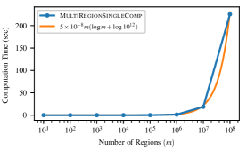
Figure 7: Running time: MultiRegionSingleComp v.s. $O(m(\log m+\log 10^{12}))$.

A similar study of checking the running time dependency over $n$ was carried out as well but did not show a tight dependency of the running time over $\log n$. This is because the $O(m\log n)$ part (from the $\mathbf{while}$ loop in MultiRegionSingleComp) is dominated by the $O(m\log m)$ part (from the enhanced $\mathbf{while}$ loop with bisection).

For the case of a single perimeter with multiple components, a random polygon is generated on which $2q$ points are randomly sampled that yield $q$ segments (that form the perimeter) and $q$ gaps. Some example instances and the optimal solutions are illustrated in Fig. 8. The computation time for various $q$ and $n$ combinations is given in Table II.

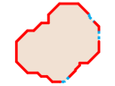
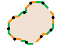
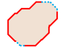
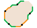
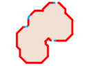
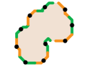
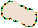
Figure 8: Four examples for the case of single region with multiple components. Problem parameters are as follows: first row, $q=3$, $n=10$; second row, $q=2$, $n=5$; third row, $q=4$, $n=10$; fourth row, $q=5$, $n=15$.

	$10^{1}$	$10^{2}$	$10^{3}$	$10^{4}$	$10^{5}$
$10^{2}$	$0.013$	$0.015$	$0.016$	$0.016$	$0.017$
$10^{3}$	$1.363$	$1.595$	$1.622$	$1.634$	$1.641$
$10^{4}$	$159.404$	$188.497$	$210.492$	$212.473$	$212.780$

TABLE II: SingleRegionMultiComp computation time (seconds)

For SingleRegionMultiComp, the dependency of the running time over $q^{2}\log q$ appears to be tight (see Fig. 9).

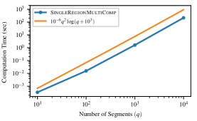
Figure 9: Running time of SingleRegionMultiComp v.s. $O(q^{2}\log(q+10^{3}))$.

For multiple perimeters containing multiple components, $m$ polygons are created with $len(\partial R_{i})$ randomly distributed in $[1,10]$. For setting $q_{i}$, we fix a $q$ and let $q_{i}=q(0.5+random(0,1))$. Representative computation results of MultiRegionMultiComp are listed in Table III.

$q$	$n$	$m$
		$10$	$20$	$30$	$40$	$50$
$10^{1}$	$10^{2}$	$0.015$	$0.027$	$0.039$	$0.045$	$0.054$
$10^{1}$	$10^{3}$	$0.047$	$0.063$	$0.076$	$0.091$	$0.108$
$10^{2}$	$10^{2}$	$1.492$	$2.784$	$4.168$	$5.404$	$6.444$
$10^{2}$	$10^{3}$	$2.191$	$3.771$	$5.523$	$7.707$	$9.369$
$10^{2}$	$10^{4}$	$7.105$	$9.619$	$11.369$	$12.760$	$15.107$

TABLE III: MultiRegionMultiComp computation time (seconds)

As for running time, Fig. 10 shows the dependency on the number of regions $m$ appears to be linear with $q$ fixed (recall we set $q_{i}=q(0.5+random(0,1))$). This is tight in viewing the main running time of MultiRegionMultiComp which is $O((\sum_{1\leq i\leq m}q_{i}^{2})\log(n+\sum_{1\leq i\leq m}q_{i}))$; if $q_{i}$ is fixed, then the time is linear with respect to $m$. An example computation result for $m=3$ is illustrated in Fig. 11.

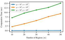
Figure 10: Running time of MultiRegionMultiComp v.s. the number of regions.

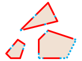
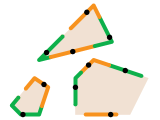
Figure 11: An example instance when $m=3$, $n=10$.

V-B Two Applications Scenarios

Securing a perimeter. As a first application, consider a situation where a crime has just been committed at the Edinburgh Castle (see Fig. 12). The culprit remains in the confines of the castle but is mixed within many guests at the scene. As the situation is being investigated and suppose that the brick colored buildings are secured, guards (either personnel or a number of drones) may be deployed to ensure the culprit does not escape by climbing down the castle walls. Using SingleRegionMultiComp, a deployment plan can be quickly computed given the amount of resources at hand so that each guard only needs to secure a minimum length along the castle walls. Fig. 12 shows the optimal deployment plan for $15$ guards.

\begin{overpic}[width=180.67499pt,tics=5]{./figures/castle_15-eps-converted-to.pdf} \end{overpic}

Figure 12: Optimal deployment of $15$ guards around walls of the Edinburgh Castle. The brick colored structures are buildings that create gaps along the boundary.

Then, Fig. 13 shows the deployment plan for $n=5,10,20,30$ guards. As the number of guards changes from $5$ to $10$, the gap on the lower left side is no longer covered due to the availability of more guards. Similarly, as the number of guards changes from $20$ to $30$, the very small gap on the top no longer needs to be covered.

\begin{overpic}[width=180.67499pt,tics=5]{./figures/castle_5-eps-converted-to.pdf} \end{overpic}

\begin{overpic}[width=180.67499pt,tics=5]{./figures/castle_10-eps-converted-to.pdf} \end{overpic}

\begin{overpic}[width=180.67499pt,tics=5]{./figures/castle_20-eps-converted-to.pdf} \end{overpic}

\begin{overpic}[width=180.67499pt,tics=5]{./figures/castle_30-eps-converted-to.pdf} \end{overpic}

Figure 13: Optimal deployment of $5,10,20,30$ guards around the Edinburgh Castle.

Fire monitoring. In a second application, consider Fig. 14 where a forest fire has just been put out in multiple regions. As there is still some chance that the fire may rekindle and spread, for prevention, a team of firefighters is to be deployed to watch for the possible spreading of the fire. Here, in addition to using MultiRegionMultiComp to compute optimal locations for deploying the firefighters, we also generate minimum time trajectories for the firefighters to reach their target locations while avoiding going through the dangerous forests. This is done via solving a bottleneck assignment problem [37]. Note that the lake region creates gaps that cannot be traveled by the firefighters; this can be handled by making these gaps infinitely large. Fig. 14 shows the optimal locations for $34$ firefighters. Animations of the deployment process and other test cases can be found in the accompanying video.

\begin{overpic}[width=180.67499pt,tics=5]{./figures/forest_solution-eps-converted-to.pdf} \end{overpic}

Figure 14: Optimal deployment of $34$ firefighters for forest fire rekindling prevention.

Additional computational results for the forest fire monitoring case is illustrated in Fig. 15. Behavior similar to that from the castle case can be observed here, e.g., from $30$ to $40$ guards, the small gap on the right is no longer covered.

\begin{overpic}[width=180.67499pt,tics=5]{./figures/forest_solution5-eps-converted-to.pdf} \end{overpic}

\begin{overpic}[width=180.67499pt,tics=5]{./figures/forest_solution10-eps-converted-to.pdf} \end{overpic}

\begin{overpic}[width=180.67499pt,tics=5]{./figures/forest_solution20-eps-converted-to.pdf} \end{overpic}

\begin{overpic}[width=180.67499pt,tics=5]{./figures/forest_solution30-eps-converted-to.pdf} \end{overpic}

\begin{overpic}[width=180.67499pt,tics=5]{./figures/forest_solution40-eps-converted-to.pdf} \end{overpic}

Figure 15: Optimal deployment of $5,10,20,30,40$ firefighters for forest fire monitoring.

VI Conclusion and Discussion

In this paper, we propose the OPG problem to model the allocation of a large number of robots to cover complex 1D topological domains with optimality guarantees. For all variants under the OPG formulation umbrella, we have developed highly efficient algorithms for solving OPG exactly. In addition to rigorous proofs backed by formal analysis, extensive computational experiments further confirm the effectiveness of these algorithms. Moreover, practical relevance of OPG is demonstrated through the integration of OPG into realistic task (assignment) and motion planning scenarios.

The study raises many additional interesting open questions; we mention a few here. First, the approach taken in this work is a centralized one where decision is made at the global level. It would be highly interesting to explore whether the same can be achieved with decentralized methods, which have many advantages. For example, it may be the case that the gaps along the boundaries are not known a priori and must be measured by the robots. In such cases, a centralized plan can be hard to come by. Second, as mentioned in Section II, the current OPG formulation assumes that the robots are confined to the boundaries $\partial\mathcal{R}$, which is one of many possible choices in terms of the robots' sensing and/or motion capabilities. In future study, we plan to examine additional practical robot sensing and motion models. Third, as exact optimal algorithms are emphasized here, issues including uncertainty and robustness have not been touched in the current treatment, which are important elements when it comes to the deployment of a robotic swarm to tackle real-world challenges.

Acknowledgments. This work is supported by NSF grants IIS-1617744, IIS-1734419, and IIS-1845888. Opinions or findings expressed in this paper do not necessarily reflect the views of the sponsors.

References

- [1] T. Arai, E. Pagello, and L. E. Parker, ``Advances in multi-robot systems,'' IEEE Transactions on robotics and automation, vol. 18, no. 5, pp. 655–661, 2002.
- [2] B. P. Gerkey and M. J. Matarić, ``A formal analysis and taxonomy of task allocation in multi-robot systems,'' The International Journal of Robotics Research, vol. 23, no. 9, pp. 939–954, 2004.
- [3] W. Ren and R. W. Beard, Distributed consensus in multi-vehicle cooperative control. Springer, 2008.
- [4] F. Bullo, J. Cortes, and S. Martinez, Distributed control of robotic networks: a mathematical approach to motion coordination algorithms. Princeton University Press, 2009, vol. 27.
- [5] H. Ando, Y. Oasa, I. Suzuki, and M. Yamashita, ``Distributed memoryless point convergence algorithm for mobile robots with limited visibility,'' IEEE Transactions on Robotics and Automation, vol. 15, no. 5, pp. 818–828, 1999.
- [6] A. Jadbabaie, J. Lin, and A. S. Morse, ``Coordination of groups of mobile autonomous agents using nearest neighbor rules,'' IEEE Transactions on automatic control, vol. 48, no. 6, pp. 988–1001, 2003.
- [7] R. Olfati-Saber and R. M. Murray, ``Consensus problems in networks of agents with switching topology and time-delays,'' IEEE Transactions on automatic control, vol. 49, no. 9, pp. 1520–1533, 2004.
- [8] W. Ren and R. W. Beard, ``Consensus seeking in multiagent systems under dynamically changing interaction topologies,'' IEEE Transactions on automatic control, vol. 50, no. 5, pp. 655–661, 2005.
- [9] P. Cheng and V. Kumar, ``An almost communication-less approach to task allocation for multiple unmanned aerial vehicles,'' in Robotics and Automation, 2008. ICRA 2008. IEEE International Conference on. IEEE, 2008, pp. 1384–1389.
- [10] M. Mesbahi and M. Egerstedt, Graph theoretic methods in multiagent networks. Princeton University Press, 2010, vol. 33.
- [11] J. Yu, S. M. LaValle, and D. Liberzon, ``Rendezvous without coordinates,'' IEEE Transactions on Automatic Control, vol. 57, no. 2, pp. 421–434, 2012.
- [12] S. L. Smith and F. Bullo, ``Monotonic target assignment for robotic networks,'' IEEE Transactions on Automatic Control, vol. 54, no. 9, pp. 2042–2057, 2009.
- [13] N. Ayanian and V. Kumar, ``Decentralized feedback controllers for multiagent teams in environments with obstacles,'' IEEE Transactions on Robotics, vol. 26, no. 5, pp. 878–887, 2010.
- [14] L. Liu and D. A. Shell, ``Multi-level partitioning and distribution of the assignment problem for large-scale multi-robot task allocation,'' Robotics: Science and Systems VII; MIT Press: Cambridge, MA, USA, pp. 26–33, 2011.
- [15] ——, ``Optimal market-based multi-robot task allocation via strategic pricing.'' in Robotics: Science and Systems, vol. 9, no. 1, 2013, pp. 33–40.
- [16] M. Turpin, K. Mohta, N. Michael, and V. Kumar, ``Goal assignment and trajectory planning for large teams of interchangeable robots,'' Autonomous Robots, vol. 37, no. 4, pp. 401–415, 2014.
- [17] M. Turpin, N. Michael, and V. Kumar, ``Capt: Concurrent assignment and planning of trajectories for multiple robots,'' The International Journal of Robotics Research, vol. 33, no. 1, pp. 98–112, 2014.
- [18] J. Alonso-Mora, S. Baker, and D. Rus, ``Multi-robot navigation in formation via sequential convex programming,'' in Intelligent Robots and Systems (IROS), 2015 IEEE/RSJ International Conference on. IEEE, 2015, pp. 4634–4641.
- [19] K. Solovey, J. Yu, O. Zamir, and D. Halperin, ``Motion planning for unlabeled discs with optimality guarantees,'' in Robotics: Science and Systems, 2015.
- [20] D. E. Soltero, M. Schwager, and D. Rus, ``Decentralized path planning for coverage tasks using gradient descent adaptive control,'' The International Journal of Robotics Research, vol. 33, no. 3, pp. 401–425, 2014.
- [21] A. Howard, M. J. Matarić, and G. S. Sukhatme, ``Mobile sensor network deployment using potential fields: A distributed, scalable solution to the area coverage problem,'' in Distributed Autonomous Robotic Systems 5. Springer, 2002, pp. 299–308.
- [22] M. Schwager, B. J. Julian, and D. Rus, ``Optimal coverage for multiple hovering robots with downward facing cameras,'' in 2009 IEEE international conference on robotics and automation. IEEE, 2009, pp. 3515–3522.
- [23] J. O'rourke, Art gallery theorems and algorithms. Oxford University Press Oxford, 1987, vol. 57.
- [24] T. C. Shermer, ``Recent results in art galleries (geometry),'' Proceedings of the IEEE, vol. 80, no. 9, pp. 1384–1399, 1992.
- [25] V. Klee, ``Is every polygonal region illuminable from some point?'' The American Mathematical Monthly, vol. 76, no. 2, pp. 180–180, 1969.
- [26] T. Lozano-Pérez and M. A. Wesley, ``An algorithm for planning collision-free paths among polyhedral obstacles,'' Communications of the ACM, vol. 22, no. 10, pp. 560–570, 1979.
- [27] D. Lee and A. Lin, ``Computational complexity of art gallery problems,'' IEEE Transactions on Information Theory, vol. 32, no. 2, pp. 276–282, 1986.
- [28] A. Thue, Über die dichteste Zusammenstellung von kongruenten Kreisen in einer Ebene, von Axel Thue… J. Dybwad, 1910.
- [29] T. C. Hales, ``A proof of the kepler conjecture,'' Annals of mathematics, pp. 1065–1185, 2005.
- [30] Z. Drezner, Facility location: a survey of applications and methods. Springer Verlag, 1995.
- [31] J. Cortes, S. Martinez, T. Karatas, and F. Bullo, ``Coverage control for mobile sensing networks,'' IEEE Transactions on robotics and Automation, vol. 20, no. 2, pp. 243–255, 2004.
- [32] M. Pavone, A. Arsie, E. Frazzoli, and F. Bullo, ``Equitable partitioning policies for robotic networks,'' in Robotics and Automation, 2009. ICRA'09. IEEE International Conference on. IEEE, 2009, pp. 2356–2361.
- [33] S. Martínez, ``Distributed interpolation schemes for field estimation by mobile sensor networks,'' IEEE Transactions on Control Systems Technology, vol. 18, no. 2, pp. 491–500, 2010.
- [34] A. Pierson, L. C. Figueiredo, L. C. Pimenta, and M. Schwager, ``Adapting to sensing and actuation variations in multi-robot coverage,'' The International Journal of Robotics Research, vol. 36, no. 3, pp. 337–354, 2017.
- [35] R. B. Kershner, ``On paving the plane,'' The American Mathematical Monthly, vol. 75, no. 8, pp. 839–844, 1968.
- [36] C. D. Toth, J. O'Rourke, and J. E. Goodman, Handbook of discrete and computational geometry. Chapman and Hall/CRC, 2017.
- [37] R. E. Burkard and E. Cela, ``Linear assignment problems and extensions,'' in Handbook of combinatorial optimization. Springer, 1999, pp. 75–149.