An $\mathcal{O}(1)$ algorithm for the numerical evaluation of the prolate spheroidal wave functions of order $0$

Abstract

The standard algorithm for the numerical evaluation of the prolate spheroidal wave function $\mathsf{Ps}\hskip 0.50003pt{}_{n}(x;\gamma^{2})$ of order $0$, bandlimit $\gamma>0$ and characteristic exponent $n$ has running time which grows with both $n$ and $\gamma$. Here, we describe an alternate approach which runs in time independent of these quantities. We present the results of numerical experiments demonstrating the properties of our scheme, and we have made our implementation of it publicly available.

The prolate spheroidal wave functions

$$\mathsf{Ps}\hskip 0.50003pt{}_{0}\left(z;\gamma^{2}\right),\mathsf{Ps}\hskip 0.50003pt{}_{1}\left(z;\gamma^{2}\right),\mathsf{Ps}\hskip 0.50003pt{}_{2}\left(z;\gamma^{2}\right),\ldots$$ (1)

are the eigenfunctions of the restricted Fourier operator

$$T_{\gamma}\left[f\right](z)=\int_{-1}^{1}\exp(i\gamma zt)f(t)\ dt.$$ (2)

As such, they provide an efficient mechanism for representing bandlimited functions, and for performing many computations related to such functions (see, for instance, [27, 17, 18, 22, 14, 26, 24, 23, 4]).

In the seminal work [27], it was observed these functions also constitute the set of solutions of a singular self-adjoint Sturm-Liouville problem. More explicitly, (1) is the collection of all eigenfunctions of the differential operator

$$L_{\gamma}\left[y\right](x)=-(1-x^{2})y^{\prime}(x)+2xy^{\prime}(x)+\gamma^{2}x^{2}y(x)$$ (3)

which satisfy the self-adjoint boundary conditions

$$\lim_{x\to 1}(1-x^{2})y^{\prime}(x)=0=\lim_{x\to-1}(1-x^{2})y^{\prime}(x).$$ (4)

In other words, each of the functions $\mathsf{Ps}\hskip 0.50003pt{}_{n}(x;\gamma^{2})$ is a solution of the spheroidal wave equation

$$(1-x^{2})y^{\prime}(x)-2xy^{\prime}(x)+(\chi-\gamma^{2}x^{2})y(x)=0$$ (5)

with $\chi$ the Sturm-Liouville eigenvalue of $\mathsf{Ps}\hskip 0.50003pt{}_{n}(x;\gamma^{2})$; we will denote this value of $\chi$ via $\chi_{n}(\gamma^{2})$.

The standard algorithm for the numerical evaluation of the functions (1) is based on discretizing the eigenproblem for the differential operator $L_{\gamma}$ rather than the eigenproblem for the integral operator $T_{\gamma}$. This approach is preferred because of the nature of the spectrum of $T_{\gamma}$ — it has roughly $2\gamma/\pi$ eigenvalues which are close to $\sqrt{2\pi/\gamma}$, on the order of $\log(\gamma)$ eigenvalues which decay rapidly to $0$ and the rest of its eigenvalues are of very small magnitude. The eigenvalues of $L_{\gamma}$ are, on the other hand, well-separated.

When the eigenproblem

$$L_{\gamma}\left[y\right](x)=\chi y(x)$$ (6)

is discretized by introducing one of the representations

$$y(x)=\sum_{k=0}^{\infty}a_{k}\mathsf{P}\hskip 0.50003pt{}_{2k}(x)$$ (7)

or

$$y(x)=\sum_{k=0}^{\infty}a_{k}\mathsf{P}\hskip 0.50003pt{}_{2k+1}(x),$$ (8)

where $\mathsf{P}\hskip 0.50003pt{}_{n}(x)$ denotes Ferrer’s version of the Legendre function of the first kind of degree $n$, the result is an infinite symmetrizable tridiagonal matrix. In the case of (7), the eigenvalues of the matrix are

$$\chi_{0}(\gamma^{2})<\chi_{2}(\gamma^{2})<\chi_{4}(\gamma^{2})<\cdots$$ (9)

while the representation (8) leads to a matrix whose spectrum consists of

$$\chi_{1}(\gamma^{2})<\chi_{3}(\gamma^{2})<\chi_{5}(\gamma^{2})<\cdots.$$ (10)

After proper normalization, the eigenvectors of these matrices give the coefficients in the Legendre expansions of the functions (1). To evaluate $\mathsf{Ps}\hskip 0.50003pt{}_{n}(x;\gamma^{2})$, its Legendre expansion is first constructed by truncating one of the two infinite matrices mentioned above, symmetrizing it, and calculating the appropriate eigenvalue and corresponding eigenvector. The fact that the matrix is symmetrizable greatly reduces the difficulty of these computations. The function $\mathsf{Ps}\hskip 0.50003pt{}_{n}(x;\gamma^{2})$ can then be evaluated at any point in the interval $(-1,1)$ via the resulting Legendre expansion.

This procedure is sometimes called the Legendre-Galerkin method, although we refer to it as the Xiao-Rokhlin algorithm as it appears to have first been described in its entirety in [33]. A part of the procedure was described earlier in [13]; there, the Sturm-Liouville eigenvalues of the prolate spheroidal wave functions are obtained in the fashion described above. However, the three-term recurrence relations satisfied by the Legendre coefficients are then used to construct the expansions of the prolate spheroidal wave functions. The resulting method does not provide a numerically stable mechanism for evaluating the functions $\mathsf{Ps}\hskip 0.50003pt{}_{n}(x;\gamma^{2})$ and extended precision arithmetic is required to produce accurate results using it, even for small values of $\gamma$ and $n$. It is often stated in the literature that the Xiao-Rokhlin procedure was first described in [6]. In fact, the method of [6] for the computation of the Sturm-Liouville eigenvalues is quite different and is based on the well-known observation that the three-term recurrence relations which arise from inserting the representations (7) and (8) into (5) are related to infinite continued fraction expansions. A thorough discussion of the Xiao-Rokhlin algorithm and related techniques can be found in [22].

We refer to the construction of the Legendre expansion as the precomputation phase of the Xiao-Rokhlin algorithm. Its running time clearly depends on the size of the tridiagonal discretization matrix formed during the procedure. The precise dimension required to achieve a specified precision for $\mathsf{Ps}\hskip 0.50003pt{}_{n}(x;\gamma)$ is not known; however, the numerical experiments described in [25] suggest that it must grow as

$$\mathcal{O}\left(n+\sqrt{n\gamma}\right)$$ (11)

in order to achieve fixed precision independent of $\gamma$ and $n$. It is likely, then, that the cost of the Xiao-Rokhlin precomputation phase is

$$\mathcal{O}\left(\left(n+\sqrt{n\gamma}\right)\log\left(n+\sqrt{n\gamma}\right)\right)$$ (12)

since one eigenvalue and eigenvector pair of an $n\times n$ symmetric tridiagonal matrix can be found in $\mathcal{O}(n\log(n))$ operations. Moreover, the cost of evaluating the resulting Legendre expansion at a single point scales linearly with the dimension of the tridiagonal matrix so that the asymptotic complexity of evaluating $\mathsf{Ps}\hskip 0.50003pt{}_{n}(x;\gamma^{2})$ at a point via the Xiao-Rokhlin method is likely $\mathcal{O}\left(n+\sqrt{n\gamma}\right)$, exclusive of the costs of the precomputation phase. Of course, there exist fast algorithms for evaluating an $n$-term Legendre expansion at certain collections of $\mathcal{O}(m)$ points in $\mathcal{O}\left(n\log(n)+m\right)$ operations. However, it is often desirable to evaluate the prolate functions at a small number of points. This is particularly true when performing calculations on parallel computers, in which case it is often preferable to perform separate evaluations on different computational units. Hence, the cost of evaluating $\mathsf{Ps}\hskip 0.50003pt{}_{n}(x;\gamma^{2})$ at a single point is of interest.

Here, we describe an algorithm for the numerical evaluation of the prolate spheroidal wave functions that runs in time independent of $n$ and $\gamma$. Like the Xiao-Rokhlin algorithm, it has a precomputation phase in which a representation of $\mathsf{Ps}\hskip 0.50003pt{}_{n}(x;\gamma^{2})$ is constructed. However, rather than a Legendre expansion, we use a nonoscillatory phase function $\mathit{\Psi S}\hskip 0.50003pt{}_{\nu}(x;\gamma^{2})$ for the differential equation (5) to represent $\mathsf{Ps}\hskip 0.50003pt{}_{n}(x;\gamma^{2})$. The cost of constructing $\mathit{\Psi S}\hskip 0.50003pt{}_{\nu}(x;\gamma^{2})$ is independent of the parameters $n$ and $\gamma$, as is the cost of evaluating $\mathsf{Ps}\hskip 0.50003pt{}_{n}(x;\gamma^{2})$ via $\mathit{\Psi S}\hskip 0.50003pt{}_{\nu}(x;\gamma^{2})$.

That such nonoscillatory phase functions exist for many second order differential equations, including (5), has long been known, and they have often been exploited to accelerate the numerical calculation of certain special functions and their zeros. For instance, [21] introduces a scheme for calculating the zeros of Bessel functions which also relies on the existence of a nonoscillatory phase function for Bessel’s differential equation, [12] suggests the use of such a phase function to evaluate the Bessel functions of large orders, and one component of the widely used algorithm of [1] for the evaluation of Bessel functions makes use of asymptotic expansions of a nonoscillatory phase function for Bessel’s differential equation. These algorithms rely on extensive analytic understanding of the nonoscillatory phase functions for Bessel’s differential equation. Similar approaches can only be applied to other classes of special function for which such extensive knowledge is available, and this has, until recently, limited the applicability of such methods to a relatively small number of cases.

In [29], an iterative method based on nonoscillatory phase functions is used to calculate the zeros of functions defined by a class of second order differential equations with polynomial coefficients. A generalization of the scheme is used in [30] to construct asymptotic expansions for the solutions of a large class of second order differential equations with polynomials coefficients, and [28] extends the method to second order differential equations with coefficients that grow exponentially fast. The schemes of [29], [30] and [28] are widely applicable, but they require the calculation of high order derivatives of the coefficients of the differential equations to which they are applied. Since these derivatives cannot be calculated numerically without severe loss of precision, the schemes of [29], [30] and [28] are carried out symbolically using computer algebra systems. They are best viewed as algorithms for the symbolic computation of asymptotic expansions of nonoscillatory phase functions.

In [7], a numerical algorithm for the calculation of nonoscillatory phase functions for a large class of second order differential equations is introduced. It runs in time independent of the frequency of oscillation of their solutions and does not require knowledge of the derivatives of the coefficients of the differential equation. This algorithm is a major component in our scheme to construct the nonoscillatory phase function for (5).

By itself, however, the algorithm of [7] is insufficient to construct $\mathit{\Psi S}\hskip 0.50003pt{}_{n}(x;\gamma^{2})$ since it requires knowledge of the Sturm-Liouville eigenvalue $\chi_{n}(\gamma^{2})$ to do so. The obvious solution is to use an asymptotic expansion for $\chi_{n}(\gamma^{2})$. Unfortunately, high accuracy asymptotic expansions of the Sturm-Liouville eigenvalues which are suitable for use in numerical codes do not appear to be available at this time. For instance, [10] and [5] describe Liouville-Green type uniform asymptotic expansions of $\chi_{n}(\gamma^{2})$ and $\mathsf{Ps}\hskip 0.50003pt{}_{n}(x;\gamma^{2})$, but they involve a complicated change of variables defined in terms of an elliptic integral. Moreover, only a few coefficients in the resulting expansions are known, which greatly limits the achievable accuracy of these expansions.

The construction of asymptotic expansions for $\chi$ and the prolate spheroidal wave functions is complicated by the fact that, when viewed as a function of the characteristic exponent $\nu$, $\chi$ has branch cuts. We give a definition of the characteristic exponent of a solution of (5) in Section 1.1; for the reader who is unfamiliar with the notion, it suffices for now to know that it describes the behavior of the solution at infinity and allows for the extension of the definitions of $\mathsf{Ps}\hskip 0.50003pt{}_{\nu}(x;\gamma^{2})$, $\mathit{\Psi S}\hskip 0.50003pt{}_{\nu}(x;\gamma^{2})$ and $\chi_{\nu}(\gamma^{2})$ to arbitrary complex values of $\nu$. Many asymptotic expressions for $\chi$ and other quantities related to the prolate spheroidal wave functions are, in effect, expansions in $\nu$, and so are attempts to approximate discontinuous functions with all of the obvious difficulties that entails.

We take a somewhat different tack and numerically construct expansions of $\chi$ and and a few other quantities as functions of the bandlimit $\gamma$ and a second parameter which is related to $\mathit{\Psi S}\hskip 0.50003pt{}_{n}(0;\gamma^{2})$, the value at $0$ of a nonoscillatory phase function representing $\mathsf{Ps}\hskip 0.50003pt{}_{n}(x;\gamma^{2})$. It is the case that

$$\mathit{\Psi S}\hskip 0.50003pt{}_{n}(0;\gamma^{2})=-\pi/2(n+1),$$ (13)

and our expansions are (essentially) functions of the parameter

$$\xi=-\frac{2}{\pi}\mathit{\Psi S}\hskip 0.50003pt{}_{\nu}(0;\gamma^{2})-1.$$ (14)

Among other things, this ensures that $\chi(\xi;\gamma^{2})$ is equal to the Sturm-Liouville eigenvalue of $\mathsf{Ps}\hskip 0.50003pt{}_{n}(x;\gamma^{2})$ when $\xi=n$. In fact, for technical reasons we will discuss in detail when we describe the numerical procedure used to construct them, these expansions are functions of a variable related to $\xi$ through $\gamma$. However, for most intents and purposes, they can be viewed as functions of $\xi$, and we will discuss as if they are. While $\chi$ is discontinuous as a function of characteristic exponent, it is smooth as a function of $\xi$. This is rather dramatically demonstrated by Figure 1, which contains plots of $\chi$ as a function of the characteristic exponent $\nu$ and of $\chi$ as a function of the parameter $\xi$ when $\gamma=500$. The other quantities we represent in this fashion are the values at $0$ of the first three derivatives of the nonoscillatory phase function $\mathit{\Psi S}\hskip 0.50003pt{}_{\nu}(x;\gamma^{2})$ with respect to the argument $x$. We will use the notations

$$\mathit{\Psi S}\hskip 0.50003pt{}_{\nu}^{\prime}(x;\gamma^{2}),\ \ \mathit{\Psi S}\hskip 0.50003pt{}_{\nu}^{\prime\prime}(x;\gamma^{2}),\ \ \mathit{\Psi S}\hskip 0.50003pt{}_{\nu}^{\prime\prime\prime}(x;\gamma^{2}),\ \ \ldots$$ (15)

to denote the derivatives of the nonoscillatory phase function with respect to $x$.

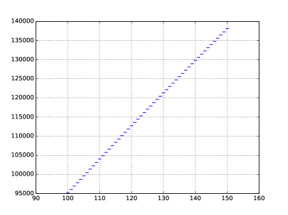
Figure 1: On the left is a plot of $\chi$ as a function of the characteristic exponent $\nu$ with $\gamma$ fixed at $500$. There is a discontinuity in the graph of this function at each half-integer value of $\nu$. On the right is a plot of $\chi$ as a function of $\xi$ with $\gamma$ again fixed at $500$. The parameter $\xi$ to the value $\mathit{\Psi S}\hskip 0.50003pt{}_{n}(0;\gamma^{2})$ of a nonoscillatory phase function for the spheroidal wave equation at $0$ through an affine mapping.

Our expansions of $\chi$ and the derivatives of the nonoscillatory phase provide a mechanism for the numerical evaluation of $\chi_{n}(\gamma^{2})$ that runs in time independent of the parameters $n$ and $\gamma$, and they give us the data necessary to calculate the nonoscillatory phase function $\mathit{\Psi S}\hskip 0.50003pt{}_{n}(x;\gamma^{2})$ representing $\mathsf{Ps}\hskip 0.50003pt{}_{n}(x;\gamma^{2})$. The time required to construct $\mathit{\Psi S}\hskip 0.50003pt{}_{n}(x;\gamma^{2})$ is independent of $n$ and $\gamma$, as is the time required to evaluate $\mathsf{Ps}\hskip 0.50003pt{}_{n}(x;\gamma^{2})$ using $\mathit{\Psi S}\hskip 0.50003pt{}_{n}(x;\gamma^{2})$.

The approach of [7] is designed for the regime in which the coefficients in (5) are sufficiently large and it loses accuracy when this is not the case. Moreover, the use of precomputed expansions means that we must a priori fix some range for the parameters $\gamma$ and $n$. The algorithm we describe here applies when

$$256=2^{8}\leq\gamma\leq 2^{20}=1,048,576\ \ \mbox{and}\ \ 200\leq n\leq\gamma.$$ (16)

That our method doesn’t apply when both $\gamma$ and $n$ are small is of little account as the Xiao-Rokhlin algorithm is highly effective in that regime. Moreover, our algorithm could be easily altered to allow for the evaluation of $\mathsf{Ps}\hskip 0.50003pt{}_{n}(x;\gamma^{2})$ in the case of larger values of $n$ and $\gamma$. That the algorithm does not apply for small $n$ and large $\gamma$, however, is a significant limitation. The authors will report on an alternate method which can be used in this regime at a later date.

The remainder of this document is organized as follows. In Section 1, we carefully establish the notation we use for the spheroidal wave function and review some well-known facts regarding them. Section 2 describe the method used to construct the expansions of $\chi$ and of the quantities

$$\mathit{\Psi S}\hskip 0.50003pt{}_{\nu}^{\prime}(0;\gamma^{2}),\ \ \mathit{\Psi S}\hskip 0.50003pt{}_{\nu}^{\prime\prime}(0;\gamma^{2}),\ \ \mbox{and}\ \ \mathit{\Psi S}\hskip 0.50003pt{}_{\nu}^{\prime\prime\prime}(0;\gamma^{2})$$ (17)

as functions of $\xi$ and $\gamma$. In Section 3, we detail our algorithm for the evaluation of $\mathsf{Ps}\hskip 0.50003pt{}_{n}(x;\gamma^{2})$. Finally, in Section 4, we present the results of numerical experiments which demonstrate the properties of our scheme.

1 Preliminaries

In this section, we set our notation for the spheroidal wave function and briefly review certain well-known facts which are used in the design of the algorithms of this paper. We state without proof many assertions regarding spheroidal wave functions. We refer the reader to [19], [15], [11], and [3] for thorough and rigorous discussions of this material.

1.1 Characteristic exponents

The functions (1) can be distinguished from other solutions of (5) through their behavior at infinity as well as by the boundary conditions (4). Indeed, $\mathsf{Ps}\hskip 0.50003pt{}_{n}(x;\gamma^{2})$ admits an expansion at infinity of the form

$$z^{\nu}\sum_{k=-\infty}^{\infty}d_{k}z^{2k}$$ (18)

with $\nu=n$, and the prolate spheroidal wave functions of order $0$ are the only solutions of (5) of this type. In general, for any values of the parameters $\gamma$ and $\chi$, (5) admits a solution which has an expansion of the form (18) around infinity. When $\nu$ is not a half-integer, there is a second independent solution which can expanded as

$$z^{1-\nu}\sum_{k=-\infty}^{\infty}d_{k}z^{2k}$$ (19)

at infinity. For half-integer values of $\nu$, the second independent solution takes on the form

$$z^{\nu}\log(z)\sum_{n=-\infty}^{\infty}d_{n}z^{2n}+z^{\nu}\sum_{n=-\infty}^{\infty}e_{n}z^{2n}$$ (20)

at infinity. The complex number $\nu$ in the expansion (18) is called a characteristic exponent for the solutions of (5). Obviously, $\nu$ is not uniquely determined by $\chi$ and $\gamma$.

This ambiguity can be resolved by considering what happens when $\gamma=0$. In that event, (5) becomes Legendre’s differential, and the relationship between $\chi$ and $\nu$ is well-known: $\chi=\nu(\nu+1)$. To define $\chi_{\nu}(\gamma^{2})$ uniquely for each $\gamma>0$ and $\nu$ which is not a half-integer, we require that $\chi_{\nu}(\gamma^{2})$ converge to $\nu(\nu+1)$ continuously as $\gamma\to 0^{+}$.

The definition of $\chi_{\nu}(\gamma^{2})$ in the case of half-integer values of $\nu$ is more complicated. Indeed, essentially all aspects of the spheroidal wave functions of half-integer orders require special attention. Since we have no need of these functions, we will always assume without further comment that $\nu$ is not a half-integer in what follows. For a definitions of $\chi_{\nu}(\gamma^{2})$ and the spheroidal wave functions in the case of half-integer values of $\nu$, we refer the reader to [19], [20] and [15].

1.2 Notations for the spheroidal wave functions

Several different notations for the spheroidal wave functions are in widespread use. For the most part, we follow Chapter 30 of [9]. In particular, we use $\mathit{Ps}\hskip 0.50003pt{}_{\nu}\left(z;\gamma^{2}\right)$ and $\mathit{Qs}\hskip 0.50003pt{}_{\nu}\left(z;\gamma^{2}\right)$ to denote the angular spheroidal wave functions of the first and second kinds of order $0$, characteristic exponent $\nu$ and bandlimit $\gamma$, respectively. The function $\mathit{Ps}\hskip 0.50003pt{}_{\nu}\left(z;\gamma^{2}\right)$ can defined via an expansion of the form

$$\sum_{k=-\infty}^{\infty}a_{\nu,k}(\gamma^{2})P_{\nu+2k}(z),$$ (21)

where $P_{\nu}$ is the Legendre function of the first kind of degree $\nu$ and the coefficients $\{a_{\nu,n}(\gamma^{2})\}$ are determined by a three-term recurrence relation. When $\nu$ is not an integer, the function $\mathit{Qs}\hskip 0.50003pt{}_{\nu}\left(z;\gamma^{2}\right)$ admits the expansion

$$\sum_{k=-\infty}^{\infty}a_{\nu,k}(\gamma^{2})Q_{\nu+2k}(z),$$ (22)

where $Q_{\mu}$ denotes the Legendre function of second kind of degree $\mu$ and the $\{a_{\nu,n}\}$ are as in (21). When viewed as a function of $\mu$, $Q_{\mu}(z)$ has simple poles at the negative integers. Consequently, the representation (22) is not viable when $\nu$ is an integer. However, for nonnegative integers $n$, $\mathit{Qs}\hskip 0.50003pt{}_{2n}(z;\gamma^{2})$ can be represented in the form

$$\sum_{k=0}^{\infty}b_{2n,k}(\gamma^{2})P_{2k+1}(z)+\sum_{k=0}^{\infty}a_{2n,k}(\gamma^{2})Q_{2k}(z)$$ (23)

with $\{a_{2n,k}(\gamma^{2})\}$ as before and $\{b_{2n,k}(\gamma^{2})\}$ a second set of coefficients which can be obtained from $\{a_{2n,k}(\gamma^{2})\}$ by solving a system of linear algebraic equations. Likewise, $\mathit{Qs}\hskip 0.50003pt{}_{2n+1}(z;\gamma^{2})$ can be represented as a sum of the form

$$\sum_{k=0}^{\infty}b_{2n+1,k}(\gamma^{2})P_{2k}(z)+\sum_{k=0}^{\infty}a_{2n+1,k}(\gamma^{2})Q_{2k+1}(z).$$ (24)

The function of the first kind $\mathit{Ps}\hskip 0.50003pt{}_{\nu}(z;\gamma^{2})$ is analytic on the cut plane $\mathbb{C}\setminus\left(-\infty,-1\right]$, and that of the second kind $\mathit{Qs}\hskip 0.50003pt{}_{\nu}(z;\gamma^{2})$ is analytic on $\mathbb{C}\setminus\left(-\infty,1\right]$.

The standard real-valued solutions of (5) on the cut $(-1,1)$ are defined for $-1<x<1$ via the formulas

$$\mathsf{Ps}\hskip 0.50003pt{}_{\nu}\left(x;\gamma^{2}\right)=\lim_{y\to 0}\mathit{Ps}\hskip 0.50003pt{}_{\nu}\left(x+iy;\gamma^{2}\right)$$ (25)

and

$$\mathsf{Qs}\hskip 0.50003pt{}_{\nu}(x;\gamma^{2})=\lim_{y\to 0^{+}}\frac{1}{2}\left(\mathit{Qs}\hskip 0.50003pt{}_{\nu}(x+iy;\gamma^{2})+\mathit{Qs}\hskip 0.50003pt{}_{\nu}(x-iy;\gamma^{2})\right).$$ (26)

They are analogs of Ferrer’s versions $\mathsf{P}\hskip 0.50003pt{}_{\nu}(x)$ and $\mathsf{Q}\hskip 0.50003pt{}_{\nu}(x)$ of the Legendre functions, which are the standard real-valued solutions of the Legendre’s differential equation defined on $(-1,1)$ (see, for instance, Chapters 14 of [9]). Clearly, $\mathsf{Ps}\hskip 0.50003pt{}_{n}(x;\gamma^{2})$ admits the expansion

$$\mathsf{Ps}\hskip 0.50003pt{}_{\nu}(x;\gamma^{2})=\sum_{k=-\infty}^{\infty}a_{\nu,k}(\gamma^{2})\mathsf{P}\hskip 0.50003pt{}_{\nu+2k}(z),$$ (27)

and for $\nu$ which are not integers, we have

$$\mathsf{Qs}\hskip 0.50003pt{}_{\nu}(x;\gamma^{2})=\sum_{k=-\infty}^{\infty}a_{\nu,k}(\gamma^{2})\mathsf{Q}\hskip 0.50003pt{}_{\nu+2k}(z).$$ (28)

Moreover, the obvious analogs of the expansions (23) and (24) for $\mathsf{Qs}\hskip 0.50003pt{}_{2n}(x;\gamma^{2})$ and $\mathsf{Qs}\hskip 0.50003pt{}_{2n+1}(x;\gamma^{2})$ also hold. The connection formula

$$\lim_{y\to 0^{+}}\mathit{Qs}\hskip 0.50003pt{}_{\nu}(x+iy;\gamma^{2})=\mathsf{Qs}\hskip 0.50003pt{}_{\nu}(x;\gamma^{2})-i\frac{\pi}{2}\mathsf{Ps}\hskip 0.50003pt{}_{\nu}(x;\gamma^{2})$$ (29)

follows readily from the analogous formula for Legendre functions (which can be found, for instance, in Chapter 14 of [9]).

We denote the radial spheroidal wave functions of the first and second kinds of bandlimit $\gamma$, characteristic exponent $\nu$ and order $0$ via $S^{(1)}_{\nu}(z;\gamma^{2})$ and $S^{(2)}_{\nu}(z;\gamma^{2})$, respectively. For values of $\nu$ which are not half-integers, they admit expansions of the form

$$S^{(1)}_{\nu}(z;\gamma^{2})=\frac{1}{A_{\nu}(\gamma^{2})}\sum_{k=-\infty}^{\infty}(-1)^{k}a_{\nu,k}(\gamma^{2})\ \sqrt{\frac{\pi}{2\gamma z}}J_{\nu+\frac{1}{2}+2k}(\gamma z),$$ (30)

and

$$S^{(2)}_{\nu}(z;\gamma^{2})=\frac{1}{A_{\nu}(\gamma^{2})}\sum_{k=-\infty}^{\infty}(-1)^{k}a_{\nu,k}(\gamma^{2})\ \sqrt{\frac{\pi}{2\gamma z}}Y_{\nu+\frac{1}{2}+2k}(\gamma z),$$ (31)

where $J_{\mu}$ and $Y_{\mu}$ denote the Bessel function of the first and second kinds of order $\mu$, respectively. The coefficients $\{a_{\nu,k}(\gamma^{2})\}$ are as in (21) and the normalizing constant $A_{\nu}(\gamma^{2})$ is defined via

$$A_{\nu}(\gamma^{2})=\sum_{k=-\infty}^{\infty}a_{\nu,k}.$$ (32)

The radial spheroidal wave function of the third kind of bandlimit $\gamma$, characteristic exponent $\nu$ and order $0$ is

$$S^{(3)}_{\nu}(x;\gamma^{2})=S^{(1)}_{\nu}(x;\gamma^{2})+iS^{(3)}_{\nu}(x;\gamma^{2}),$$ (33)

and it admits the expansion

$$S^{(3)}_{\nu}(z;\gamma^{2})=\frac{1}{A_{\nu}(\gamma^{2})}\sum_{k=-\infty}^{\infty}(-1)^{k}a_{\nu,k}(\gamma^{2})\ \sqrt{\frac{\pi}{2\gamma z}}H^{(1)}_{\nu+\frac{1}{2}+2k}(\gamma z)$$ (34)

with $H^{(1)}_{\mu}(z)$ the Hankel function of the first kind of order $\mu$. The radial spheroidal wave functions are analytic in the cut plane $\mathbb{C}\setminus\left(-\infty,0\right]$.

It is in our notation for the Sturm-Liouville eigenvalues that we deviate from [9]. There, $\lambda_{\nu}(\gamma^{2})$ is used to denote the Sturm-Liouville eigenvalue of $\mathsf{Ps}\hskip 0.50003pt{}_{\nu}(x;\gamma^{2})$ with respect to the operator

$$\widetilde{L}_{\gamma}\left[y\right](x)=-(1-x^{2})y^{\prime}(x)+2xy^{\prime}(x)-\gamma^{2}(1-x^{2})y(x),$$ (35)

whereas we use $\chi_{\nu}(\gamma^{2})$ to denote the Sturm-Liouville eigenvalue of $\mathsf{Ps}\hskip 0.50003pt{}_{\nu}(x;\gamma^{2})$ with respect to the operator $L_{\gamma}$ defined in (3). Obviously, $\chi_{\nu}(\gamma^{2})$ is related to $\lambda_{\nu}(\gamma^{2})$ via

$$\chi_{\nu}(\gamma^{2})=\lambda_{\nu}(\gamma^{2})+\gamma^{2}.$$ (36)

Our convention is consistent with [22] and [11].

1.3 Phase functions for second order differential equations

We say that a smooth function $\alpha$ is a phase function for a second order differential equation of the form

$$y^{\prime\prime}(x)+q(x)y(x)=0\ \ \ \mbox{for all}\ \ a<x<b$$ (37)

provided $\alpha^{\prime}(x)>0$ for $a<x<b$ and the functions

$$u(x)=\frac{\sin\left(\alpha(x)\right)}{\sqrt{\alpha^{\prime}(x)}}$$ (38)

and

$$v(x)=\frac{\cos\left(\alpha(x)\right)}{\sqrt{\alpha^{\prime}(x)}}$$ (39)

constitute a basis in the space of solutions of (37). Any second order differential equation can be converted into the form (37) via a simple transformations. For instance, if $y$ satisfies (5) on $-1<x<1$, then

$$\varphi(x)=y(x)\sqrt{1-x^{2}}$$ (40)

solves

$$\varphi^{\prime\prime}(x)+q(x)\varphi(x)=0\ \ \ \mbox{for all}\ \ -1<x<1,$$ (41)

with $q$ given by

$$q(x)=\frac{1}{(1-x^{2})^{2}}+\frac{\chi-\gamma^{2}x^{2}}{1-x^{2}}.)$$ (42)

We refer to (41) as the normal form of the spheroidal wave equation.

Any pair of real-valued solutions of (37) whose Wronskian is $1$ determines a phase function for (37) up to a constant multiple of $2\pi$. Indeed, (38) and (39) immediately imply

$$\alpha^{\prime}(t)=\frac{1}{(u(t))^{2}+(v(t))^{2}},$$ (43)

which determines $\alpha$ up to a constant and that constant is fixed modulo $2\pi$ by the requirement that (38) and (39) hold.

1.4 Connection formulas for the radial spheroidal wave functions

By examining the series expansions of the spheroidal wave functions and the angular wave functions at infinity, formulas connecting the two can be obtained. Of particular interest to us are connection formulas for the radial spheroidal wave functions of the third kind of integer characteristic exponents. The boundary values of these functions on the real line give rise to a pair of real-valued solutions of (5) which generate the nonoscillatory phase functions $\mathit{\Psi S}\hskip 0.50003pt{}_{n}(x;\gamma^{2})$ we use to represent the prolate spheroidal wave functions $\mathsf{Ps}\hskip 0.50003pt{}_{n}(x;\gamma^{2})$.

In the case of nonnegative even integer characteristic exponents we have

$$S^{(1)}_{2n}(z;\gamma^{2})=K_{2n}^{(1)}(\gamma^{2})\mathit{Ps}\hskip 0.50003pt{}_{2n}(z;\gamma^{2})$$ (44)

and

$$S^{(2)}_{2n}(z;\gamma^{2})=K_{2n}^{(2)}(\gamma^{2})\mathit{Qs}\hskip 0.50003pt{}_{2n}(z;\gamma^{2}),$$ (45)

where

$$K_{2n}^{(1)}(\gamma^{2})=\frac{(-1)^{n}}{A_{2n}(\gamma^{2})}\frac{a_{2n,-n}(\gamma^{2})}{\mathsf{Ps}\hskip 0.50003pt{}_{2n}(0;\gamma^{2})}$$ (46)

and

$$K_{2n}^{(2)}(\gamma^{2})=\frac{(-1)^{n+1}}{\gamma A_{2n}(\gamma^{2})}\frac{\mathsf{Ps}\hskip 0.50003pt{}_{2n}(0;\gamma^{2})}{a_{2n,-n}(\gamma^{2})}.$$ (47)

In the case of nonnegative odd integer characteristic exponents,

$$S^{(1)}_{2n+1}(z;\gamma^{2})=K_{2n+1}^{(1)}(\gamma^{2})\mathit{Ps}\hskip 0.50003pt{}_{2n+1}(z;\gamma^{2})$$ (48)

and

$$S^{(2)}_{2n+1}(z;\gamma^{2})=K_{2n+1}^{(2)}(\gamma^{2})\mathit{Qs}\hskip 0.50003pt{}_{2n+1}(z;\gamma^{2}),$$ (49)

where

$$K_{2n+1}^{(1)}(\gamma^{2})=\frac{(-1)^{n}}{A_{2n+1}(\gamma^{2})}\frac{\gamma}{3}\frac{a_{2n+1,-n}(\gamma^{2})}{\mathsf{Ps}\hskip 0.50003pt{}_{2n+1}^{\prime}(0;\gamma^{2})}$$ (50)

and

$$K_{2n+1}^{(2)}(\gamma^{2})=\frac{(-1)^{n+1}}{\gamma A_{2n}(\gamma^{2})}\frac{3}{\gamma^{2}}\frac{\mathsf{Ps}\hskip 0.50003pt{}_{2n+1}^{\prime}(0;\gamma^{2})}{a_{2n+1,-n}(\gamma^{2})}.$$ (51)

Here, we are using the convention that the prime symbol indicates differentiation with respect to the argument $x$ so that $\mathsf{Ps}\hskip 0.50003pt{}_{2n+1}^{\prime}(0;\gamma^{2})$ denotes the value of the derivative with respect to $x$ of $\mathsf{Ps}\hskip 0.50003pt{}_{2n+1}(x;\gamma^{2})$ at $0$. For any nonnegative integer value of $n$ we have, by virtue of the preceding formulas and (29),

$$\lim_{y\to 0^{+}}S^{(3)}_{n}(x+iy;\gamma^{2})=D_{n}^{(1)}(\gamma^{2})\mathsf{Ps}\hskip 0.50003pt{}_{n}(x;\gamma^{2})+iD_{n}^{(2)}(\gamma^{2})\mathsf{Qs}\hskip 0.50003pt{}_{n}(x;\gamma^{2}),$$ (52)

where

$$D_{n}^{(1)}(\gamma^{2})=K_{n}^{(1)}(\gamma^{2})+\frac{\pi}{2}K_{n}^{(2)}(\gamma^{2})$$ (53)

and

$$D_{n}^{(2)}(\gamma^{2})=K_{n}^{(2)}(\gamma^{2}).$$ (54)

For noninteger values of $\nu$, there also exist coefficients $D_{\nu}^{(1)}(\gamma^{2})$ and $D_{\nu}^{(2)}(\gamma^{2})$ such that

$$\lim_{y\to 0^{+}}S^{(3)}_{\nu}(x+iy;\gamma^{2})=D_{\nu}^{(1)}(\gamma^{2})\mathsf{Ps}\hskip 0.50003pt{}_{\nu}(x;\gamma^{2})+iD_{\nu}^{(2)}(\gamma^{2})\mathsf{Qs}\hskip 0.50003pt{}_{\nu}(x;\gamma^{2}).$$ (55)

Their definitions, which are somewhat more complicated than in the case of integer characteristic exponents, can be found in Section 3.66 of [19].

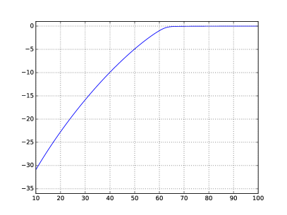
Figure 2: A plot of the base-10 logarithm of $A_{\nu}(\gamma^{2})$ as a function of $\nu$ when $\gamma=100$.

The Wronskian of the pair of solutions $\mathsf{Ps}\hskip 0.50003pt{}_{\nu}(x;\gamma^{2})$, $\mathsf{Qs}\hskip 0.50003pt{}_{\nu}(x;\gamma^{2})$ is

$$\frac{A_{\nu}^{2}(\gamma^{2})}{1-x^{2}}.$$ (56)

When $n$ is small relative to $\gamma$, the magnitude of $A_{\nu}(\gamma^{2})$ is extremely small. See, for instance, Figure 2, which contains a plot of the base-10 logarithm of $A_{\nu}(\gamma^{2})$ as a function of $\nu$ when $\gamma=100$. Among other things it shows that when $\gamma=100$, the magnitude of $A_{\nu}(\gamma^{2})$ already falls below $10^{-30}$. The situation becomes even worse as $\gamma$ increases. Clearly, the pair $\mathsf{Ps}\hskip 0.50003pt{}_{\nu}(x;\gamma^{2})$ and $\mathsf{Qs}\hskip 0.50003pt{}_{\nu}(x;\gamma^{2})$ constitute a basis which is extremely ill-conditioned numerically for many values of $\nu$ and $\gamma$. This motivates the following definitions. We let

$$C^{(1)}_{\nu}(\gamma^{2})=\frac{1}{A_{\nu}(\gamma^{2})}D^{(1)}_{\nu}(\gamma^{2})$$ (57)

and

$$C^{(2)}_{\nu}(\gamma^{2})=\frac{1}{A_{\nu}(\gamma^{2})}D^{(2)}_{\nu}(\gamma^{2}),$$ (58)

so that

$$u_{\nu}(x;\gamma^{2})=C^{(1)}_{\nu}(\gamma^{2})\mathsf{Ps}\hskip 0.50003pt{}_{\nu}(x;\gamma^{2})\sqrt{1-x^{2}}$$ (59)

and

$$v_{\nu}(x;\gamma^{2})=C^{(2)}_{\nu}(\gamma^{2})\mathsf{Qs}\hskip 0.50003pt{}_{\nu}(x;\gamma^{2})\sqrt{1-x^{2}}$$ (60)

is a pair of solutions of the normalized spheroidal wave equation (41) whose Wronskian is $1$.

Remark 1.

The numerical evaluation of the coefficients $C^{(1)}_{\nu}(\gamma^{2})$ and $C^{(2)}_{\nu}(\gamma^{2})$ through the formulas (57), (58) (53) and (54) is problematic. When $\gamma$ is of large magnitude $n$ is small relative to $\gamma$, the evaluation of these formulas using finite precision arithmetic results in catastrophic cancellation errors. In fact, when $\gamma$ is of large magnitude, this is the case even for relatively large values of $n$ (for instance, $\gamma=1000$ and $n=500$). We do not make use of these formulas in the algorithm of this paper.

1.5 The nonoscillatory phase function for the spheroidal wave equation

It follows from the formula

$$S^{(3)}_{\nu}(z)=-\frac{\exp\left(-i\frac{\pi}{2}\nu\right)}{A_{\nu}(\gamma^{2})}\int_{1}^{\infty}\exp(i\gamma zt)\mathsf{Ps}\hskip 0.50003pt{}_{\nu}(t;\gamma^{2})\ dt,$$ (61)

which specifies the Fourier transform of the radial spheroidal wave function of the third kind and can be found in Section 3.84 of [19], that the function

$$f(x)=\lim_{y\to 0^{+}}\left|S^{(3)}_{\nu}(x+iy;\gamma^{2})\right|^{2}$$ (62)

is absolutely monotone on the interval $(-1,1)$. That is, $f(x)$ and its derivatives of all orders are positive on $(-1,1)$. Indeed, this result can be obtained by using (61) to derive a formula expression the Laplace transform of the boundary value of

$$\left|S^{(3)}_{\nu}(x+iy;\gamma^{2})\right|^{2}$$ (63)

as a convolution of angular spheroidal wave functions of the first kind.

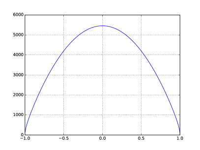
Figure 3: On the left is a plot of $\mathit{\Psi S}\hskip 0.50003pt{}_{\nu}^{\prime}(x;\gamma^{2})$ when $\gamma=500$ and $\nu=400$, and on the right is a plot of $\mathit{\Psi S}\hskip 0.50003pt{}_{\nu}^{\prime}(x;\gamma^{2})$ when $\gamma=5000$ and $\nu=4000$.

We use $\mathit{\Psi S}\hskip 0.50003pt{}_{\nu}(x;\gamma^{2})$ to denote a phase function for the normal form of the spheroidal wave equation (41) which gives rise to the solutions (59) and (60) via the formulas

$$u_{\nu}(x;\gamma^{2})=\frac{\sin\left(\mathit{\Psi S}\hskip 0.50003pt{}_{\nu}(x;\gamma^{2})\right)}{\sqrt{\mathit{\Psi S}\hskip 0.50003pt{}_{\nu}^{\prime}(x;\gamma^{2})}}$$ (64)

and

$$v_{\nu}(x;\gamma^{2})=\frac{\cos\left(\mathit{\Psi S}\hskip 0.50003pt{}_{\nu}(x;\gamma^{2})\right)}{\sqrt{\mathit{\Psi S}\hskip 0.50003pt{}_{\nu}^{\prime}(x;\gamma^{2})}}.$$ (65)

We uniquely determine $\mathit{\Psi S}\hskip 0.50003pt{}_{\nu}(x;\gamma^{2})$ by requiring that

$$\lim_{x\to 1^{-}}\mathit{\Psi S}\hskip 0.50003pt{}_{\nu}(x;\gamma^{2})=0.$$ (66)

We note that the derivative of $\mathit{\Psi S}\hskip 0.50003pt{}_{\nu}(x;\gamma^{2})$ with respect to $x$ is positive, so $\mathit{\Psi S}\hskip 0.50003pt{}_{\nu}(x;\gamma^{2})$ is a negative function which increases to $0$ as $x\to 1$ from the left. According to (43),

$$\mathit{\Psi S}\hskip 0.50003pt{}_{\nu}^{\prime}(x;\gamma^{2})=\frac{1}{\left(u_{\nu}(x;\gamma^{2})\right)^{2}+\left(v_{\nu}(x;\gamma^{2})\right)^{2}},$$ (67)

where we are once again using the convention that the prime symbol denotes differentiation with respect to the argument $x$. From (59) and (60) is is clear that the reciprocal of (67)

$$W_{\nu}(x;\gamma^{2})=\left(u_{\nu}(x;\gamma^{2})\right)^{2}+\left(v_{\nu}(x;\gamma^{2})\right)^{2}$$ (68)

is a constant multiple of

$$\left|\lim_{y\to 0^{+}}S^{(3)}_{\nu}(x+iy;\gamma^{2})\right|^{2}(1-x^{2}).$$ (69)

In particular, $\mathit{\Psi S}\hskip 0.50003pt{}_{\nu}(x;\gamma^{2})$ is nonoscillatory in the sense that the reciprocal of its derivative is equal to $(1-x^{2})$ times an absolutely monotone function. This is an extremely strong notion of “nonoscillatory,” and while many second order differential equations admit a phase function which is nonoscillatory in some sense, it is rare that they admit a phase function which is related by a sequence of algebraic operations to an absolutely monotone or completely monotone function. See [8] for a much more general notion of nonoscillatory phase function which applies to a large class of second order differential equations. Figure 3 contains the plots of the derivative of $\mathit{\Psi S}\hskip 0.50003pt{}_{\nu}(x;\gamma^{2})$ for two different pairs of the parameters $\gamma$ and $\nu$.

Remark 2.

Formula (61) follows from and is an analog of

$$\sqrt{\frac{\pi}{2z}}H^{(1)}_{\nu+\frac{1}{2}}(z)=-\exp\left(-i\frac{\pi}{2}\nu\right)\int_{1}^{\infty}\exp(izt)\mathsf{P}_{\nu}(t)\ dt,$$ (70)

which specifies the Fourier transform of the spherical Hankel function of the first kind of degree $\nu$. From (70) and standard results regarding the Fourier transform, it follows that

$$\left|\sqrt{\frac{\pi}{2z}}H^{(1)}_{\nu+\frac{1}{2}}(z)\right|^{2}=\int_{0}^{\infty}\exp(izt)\mathsf{P}_{\nu}\left(1+\frac{t^{2}}{2}\right)\ dt,$$ (71)

which can be rearranged as

$$\frac{1}{z}J_{\nu+\frac{1}{2}}^{2}(z)+\frac{1}{z}Y_{\nu+\frac{1}{2}}^{2}(z)=\frac{2}{\pi}\int_{0}^{\infty}\exp(-zt)\mathsf{P}_{\nu}\left(1+\frac{t^{2}}{2}\right)\ dt.$$ (72)

Since $\mathsf{P}_{\nu}(t)$ is nonnegative on $(1,\infty)$, we have that

$$\frac{1}{z}J_{\nu+\frac{1}{2}}^{2}(z)+\frac{1}{z}Y_{\nu+\frac{1}{2}}^{2}(z)$$ (73)

is completely monotone on the interval $(0,\infty)$. A smooth function $f$ is completely monotone on an interval $(a,b)$ if

$$(-1)^{k}f^{(k)}(x)\geq 0$$ (74)

for $x\in(a,b)$ and all nonnegative integers $k$. A function is completely monotone on $(0,\infty)$ if and only if it is the Laplace transform of a positive Borel measure. The function (73) is the reciprocal of the derivative of a phase function for the normal form

$$y^{\prime\prime}(t)+\left(1+\frac{\frac{1}{4}-\nu^{2}}{t^{2}}\right)y(t)=0$$ (75)

of Bessel’s differential equation. So the normal form of Bessel’s differential equation admits a phase function whose derivative is the reciprocal of a completely monotone function. We note that Formula (72) is an analog of Nicholson’s classical integral representation formula (see Section 13.73 of [32]), which also implies that (73) is completely monotone.

1.6 Kummer’s equation, Riccati’s equation and Appell’s equation

We now briefly discuss three differential equations which can be solved to calculate phase functions for (37). The second order nonlinear ordinary differential

$$(\alpha^{\prime}(x))^{2}=q(x)-\frac{1}{2}\frac{\alpha^{\prime\prime\prime}(x)}{\alpha^{\prime}(x)}+\frac{3}{4}\left(\frac{\alpha^{\prime\prime}(x)}{\alpha^{\prime}(x)}\right)^{2}$$ (76)

satisfied by the derivative of phase functions for (37) can be obtained from (43) through repeated differentiation. We refer to (76) as Kummer’s equation after E. E. Kummer who studied it in [16]. Kummer’s equation can also be obtained by decomposing the Riccati equation

$$r^{\prime}(x)+(r(x))^{2}+q(x)=0$$ (77)

satisfied by the logarithmic derivatives of solutions of (37) into real and imaginary parts. It can be verified through direct computation that if $u$ and $v$ are solutions of (37) then

$$w(x)=(u(x))^{2}+(v(x))^{2}$$ (78)

solves

$$w^{\prime\prime\prime}(x)+4q(x)w^{\prime}(x)+2q^{\prime}(x)w(t)=0.$$ (79)

We refer to (79) as Appell’s equation, after P. Appell who discussed it in [2].

The scaled phase function

$$\mathit{\Psi S}\hskip 0.50003pt{}_{\nu}(x;\gamma^{2})\sqrt{1-x^{2}}$$ (80)

satisfies Kummer’s equation (76) with $q$ as in (42), while the function $W_{\nu}(x;\gamma^{2})$ defined via (68) satisfies Appell’s equation (79) with $q$ as in (42).

1.7 Chebyshev expansions

An nth order univariate Chebyshev expansion on the interval $(a,b)$ is a sum of the form

$$\sum_{i=0}^{n}\beta_{i}\ T_{i}\left(\frac{2}{b-a}x-\frac{b+a}{b-a}\right),$$ (81)

where $T_{m}(x)=\cos(m\arccos(x))$ is the Chebyshev polynomial of degree $m$. We refer to the collection of points $t_{0},t_{1},\ldots,t_{n}$ defined by

$$t_{j}=\cos\left(\frac{j\pi}{n}\right),\ \ j=0,1,\ldots,n$$ (82)

as the nth order Chebyshev grid on the interval $[-1,1]$, and the set of points

$$\frac{b-a}{2}t_{j}+\frac{b+a}{2},\ \ j=0,1,\ldots,n$$ (83)

as the (n+1)-point Chebyshev grid on the interval $[a,b]$. For any continuous function $f:[a,b]\to\mathbb{R}$, we call the unique expansion of the form (81) which agrees with $f$ at the nodes (83) the nth order Chebyshev expansion of $f$ on $[a,b]$. When $f$ is infinitely differentiable, the nth order Chebyshev expansion of $f$ on $[a,b]$ converges to $f$ in the $C(\left[a,b\right])$ norm superalgebraically as n increases, and it converges to $f$ exponentially fast if $f$ is analytic in neighborhood of the interval $[a,b]$. The widespread use of Chebyshev expansions (and expansions in other families of orthogonal polynomials) in numerical calculations is principally due to their favorable stability properties. The coefficients in the Chebyshev expansion of $f$ on $[a,b]$ can be computed in a numerically stable fashion from the values of $f$ at the nodes of the Chebyshev grid on $[a,b]$, and (81) is well-conditioned as a function of the coefficients $\{\beta_{i}\}$. We refer the reader to [31] for a thorough treatment of these and other related results in approximation theory.

An nth order bivariate Chebyshev expansion on the rectangle $(a,b)\times(c,d)$ is a sum of the form

$$\sum_{0\leq i+j\leq n}\beta_{i,j}T_{i}\left(\frac{2}{b-a}x-\frac{b+a}{b-a}\right)T_{j}\left(\frac{2}{d-c}y-\frac{d+c}{d-c}\right),$$ (84)

and we call the collection of points

$$\left(\frac{b-a}{2}t_{i}+\frac{b+a}{2},\frac{d-c}{2}t_{j}+\frac{d+c}{2}\right),\ \ \ i,j=0,1,\ldots,m$$ (85)

where $t_{0},t_{1},\ldots,t_{n}$ are as in (82), the nth order Chebyshev grid on the rectangle $(a,b)\times(c,d)$. For any continuous function $f:[a,b]\to\mathbb{R}$, we call the unique expansion of the form (84) which agrees with $f$ at the nodes (85) the nth order bivariate Chebyshev expansion of $f$ on $[a,b]$. The coefficients in such an expansion can be computed in a numerical stable fashion from the values of $f$ at the nodes (85), and the expansion (84) is well-conditioned as a function of its coefficients. As in the case of univariate Chebyshev expansions, the $n$th order bivariate Chebyshev expansion of an infinitely differentiable function $f$ converges to $f$ superalgrebraically with increasing $n$, and the analyticity of $f$ in a neighborhood of implies exponential convergence.

The nth order piecewise Chebyshev expansion of the continuous function $f:[a,b]\to\mathbb{R}$ with respect to the partition

$$a=a_{1}<a_{2}<\ldots<a_{m}=b$$ (86)

of $[a,b]$ consists of the nth order Chebyshev expansions of $f$ on each of the intervals

$$(a_{1},a_{2}),(a_{2},a_{3}),\ldots,(a_{m-1},a_{m}).$$ (87)

The nth order piecewise bivariate Chebyshev expansion of the continuous function $f:[a,b]\times[c,d]\to\mathbb{R}$ with respect to the partitions

$$a=a_{1}<a_{2}<\ldots<a_{m_{1}}=b$$ (88)

and

$$c=c_{1}<c_{2}<\ldots<c_{m_{1}}=d$$ (89)

consists of the nth order bivariate Chebyshev expansions of $f$ on each of the rectangles

$$[a_{i},a_{i+1}]\times[c_{j},c_{j+1}],\ \ i=0,1,\ldots,m_{1}-1,\ \ j=0,1,\ldots,m_{2}-1.$$ (90)

We generally prefer the use of piecewise expansions to a single high order expansion for two reasons: they are more flexible in that a larger class of functions (including many singular functions) can be represented efficiently using piecewise expansions, and, perhaps more importantly for this work, the cost of evaluating a piecewise expansion at a single point is generally much lower.

1.8 Adaptive Chebyshev Discretization

We now briefly describe a fairly standard procedure for adaptively discretizing a smooth function $f:[a,b]\to\mathbb{R}$. It takes as input a desired precision $\epsilon>0$, a positive integer $n$ and a subroutine for evaluating $f$. The goal of this procedure is to construct a partition

$$a=a_{1}<a_{2}<\cdots<\gamma_{m}=b$$ (91)

of $[a,b]$ such that the $n$th order Chebyshev expansion of $f$ on each of the subintervals $[a_{j},a_{j+1}]$ approximates $f$ with accuracy $\epsilon$. That is, for each $j=1,\ldots,m-1$ we aim to achieve

$$\sup_{x\in[a_{j},a_{j+1}]}\left|f(x)-\sum_{i=0}^{n}\beta_{i,j}T_{i}\left(\frac{2}{a_{j+1}-a_{j}}x+\frac{a_{j+1}+a_{j}}{a_{j}-a{j+1}}\right)\right|<\epsilon,$$ (92)

where $\beta_{0,j},b_{1,j}\ldots,\beta_{n,j}$ are the coefficients in the $n$th order Chebyshev expansion of $f$ on the interval $\left[a_{j},a_{j+1}\right]$.

During the procedure, two lists of subintervals are maintained: a list of subintervals which are to be processed and a list of output subintervals. Initially, the list of subintervals to be processed consists of $[a,b]$ and the list of output subintervals is empty. The procedure terminates when the list of subintervals to be processed is empty or when the number of subintervals in this list exceeds a present limit (we usually take this limit to be $300$). In the latter case, the procedure is deemed to have failed. As long as the list of subintervals to process is nonempty and its length does not exceed the preset maximum, the algorithm proceeds by removing a subinterval $\left[\eta_{1},\eta_{2}\right]$ from that list and performing the following operations:

1. Compute the coefficients $\beta_{0},\ldots,\beta_{n}$ in the nth order Chebyshev expansion of the restriction of $f$ on the $[\eta_{1},\eta_{2}]$.

2. Compute the quantity

   $$\Delta=\frac{\max\left\{\left|\beta_{\frac{n}{2}+1}\right|,\left|\beta_{\frac{n}{2}+2}\right|,\ldots,\left|\beta_{n}\right|\right\}}{\max\left\{\left|\beta_{0}\right|,\left|\beta_{1}\right|,\ldots,\left|\beta_{n}\right|\right\}}.$$ (93)

3. If $\Delta<\epsilon$ then the subinterval $\left[\eta_{1},\eta_{2}\right]$ is added to the list of output subintervals.

4. If $\Delta\geq\epsilon$, then the subintervals

   $$\left[\eta_{1},\frac{\eta_{1}+\eta_{2}}{2}\right]\ \ \mbox{and}\ \ \left[\frac{\eta_{1}+\eta_{2}}{2},\eta_{2}\right]$$ (94)

   are added to the list of subintervals to be processed.

This algorithm is heuristic in the sense that there is no guarantee that (92) will be achieved, but similar adaptive discretization procedures are widely used with great success.

There is one common circumstance which leads to the failure of this procedure. The quantity $\Delta$ is an attempt to estimate the relative accuracy with which the Chebyshev expansion of $f$ on the interval $\left[\eta_{1},\eta_{2}\right]$ approximates $f$. In cases in which the condition number of the evaluation of $f$ — whose value at the point $x$ is

$$\left|x\frac{f^{\prime}(x)}{f(x)}\right|$$ (95)

— is larger than $\epsilon$ on some part of $[a,b]$, the procedure will generally fail or an excessive number of subintervals will be generated. Particular care needs to be taken when $f$ has a zero in $[a,b]$. In most cases, for $x$ near a zero of $f$, the condition number of evaluation of $f(x)$ is large. In this article, we avoid such difficulties by only applying this procedure to functions which are bounded away from $0$.

2 Numerical construction of the expansions of $\chi$ and the values of the derivatives of the nonoscillatory phase function at $0$

In this section, we describe the method which was used to construct the expansions of $\chi$ and the values

$$\mathit{\Psi S}\hskip 0.50003pt{}_{\nu}^{\prime}(0;\gamma^{2}),\ \ \mathit{\Psi S}\hskip 0.50003pt{}_{\nu}^{\prime\prime}(0;\gamma^{2}),\ \ \mbox{and}\ \ \mathit{\Psi S}\hskip 0.50003pt{}_{\nu}^{\prime\prime\prime}(0;\gamma^{2})$$ (96)

of the first few derivatives of the nonoscillatory phase function at $0$. Our expansions are functions of $\gamma$ and a parameter which is closely related to the quantity $\xi$ defined via (14). They take the form of bivariate Chebyshev expansions of order $k=29$. After their construction, they were written to a Fortran file on the disk for later use by the algorithm of Section 3; each of them expansions occupies approximately $1.1$ megabyte of memory. The computations described here were carried out on workstation equipped with $28$ Intel Xeon E5-2697 processor cores running at 2.6 GHz. They took approximately $20$ minutes to complete.

Our procedure made extensive use of the algorithm of [7], which allowed us to calculate the nonoscillatory phase function $\mathit{\Psi S}\hskip 0.50003pt{}_{\nu}(x;\gamma^{2})$ and its first few derivatives given $\gamma$ and the value of $\chi_{\nu}(\gamma^{2})$. In particular, we used it as a mechanism for evaluating

$$\mathit{\Psi S}\hskip 0.50003pt{}_{\nu}(0;\gamma^{2}),\ \ \mathit{\Psi S}\hskip 0.50003pt{}_{\nu}^{\prime}(0;\gamma^{2}),\ \ \mathit{\Psi S}\hskip 0.50003pt{}_{\nu}^{\prime\prime}(0;\gamma^{2})\ \ \mbox{and}\ \ \mathit{\Psi S}\hskip 0.50003pt{}_{\nu}^{\prime\prime\prime}(0;\gamma^{2})$$ (97)

as functions of $\gamma$ and $\chi$.

Our procedure began by introducing the partition

$$2^{8}<2^{9}<2^{10}<\ldots<2^{18}<2^{19}<2^{20}$$ (98)

of the interval

$$256=2^{8}\leq\gamma\leq 2^{20}=1,048,576.$$ (99)

We then formed the $(k+1)$-point Chebyshev grid on each of the intervals defined by this partition. For each $\gamma$ in the resulting collection of points, we performed the following sequence of operations:

1. We adaptively discretized the functions (97) with respect to the variable $\chi$ (with $\gamma$ held constant) over the interval

   $$\chi_{\xi_{1}}(\gamma^{2})\leq\chi\leq\chi_{\xi_{2}}(\gamma^{2}),$$ (100)

   where $\xi_{1}=200$ and $\xi_{2}=\gamma$. Recall, that our expansions are meant to apply in the the case of values of the parameter $\xi$ defined via (14) between $200$ and $\gamma$. The scheme of Section 1.8 was used to perform this task; the order for the Chebyshev expansions was taken to be $k$ and the requested precision was $\epsilon=10^{-14}$. The result was a partition

   $$\eta_{1}<\eta_{2}<\ldots<\eta_{m}$$ (101)

   of (100), and the $k$th order piecewise Chebyshev expansions of the functions listed in (97) with respect to this partition. We refer to the expansion of the value of the phase function via $\alpha(\chi)$, the expansion of its second derivative via $\alpha^{\prime}(\chi)$, and so on.

2. We next defined a function $\xi(\chi)$ via

   $$\xi(\chi)=-\frac{2}{\pi}\alpha(\chi)-1.$$ (102)

   Because of (13), the image of the interval (100) under this mapping is $[\xi_{1},\xi_{2}]$. We next formed the partition

   $$\sigma_{1}<\sigma_{2}<\ldots<\sigma_{m}$$ (103)

   of $[\xi_{1},\xi_{2}]$ by letting

   $$\sigma_{i}=\xi(\eta_{i}),$$ (104)

   and constructed the $k$th order piecewise Chebyshev expansion of the inverse function $\chi(\xi)$ of $\xi(\chi)$ with respect to this partition. We did so by computing the value of $\chi$ at each Chebyshev node via the most primitive root-finding method imaginable: bisection. The value of $\chi$ increases monotonically with increasing $\xi$, which made these computations significantly simpler.

   The inverse function of a polynomial of degree $k$ obviously need not be a polynomial of degree $k$, and so the piecewise Chebyshev expansion of the inverse function produced by a procedure of this sort can fail to accurately represent it, even if the piecewise Chebyshev expansion of the original function is highly accurate. We relied on the facts that the functions being inverted are extremely smooth, and that the discretizations formed by the procedure of Section 1.8 are somewhat oversampled. Moreover, we carefully verified the expansions of the inverse functions generated in this step.

3. We then defined a new parameter $\zeta$ (whose role will be made clear shortly via

   $$\xi=\xi_{1}+(\xi_{2}-\xi_{1})\zeta,$$ (105)

   so that as $\zeta$ ranges over $(0,1)$, $\xi$ ranges over $(\xi_{1},\xi_{2})$. We introduced the partition

   $$\zeta_{1}<\zeta_{2}<\ldots<\zeta_{m}$$ (106)

   of the interval $(0,1)$ which corresponds to (103) and formed $k$th order piecewise Chebyshev expansions of the functions

   $$\chi(\zeta),\ \ \alpha^{\prime}(\zeta),\ \ \alpha^{\prime\prime}(\zeta),\ \mbox{and}\ \ \alpha^{\prime\prime}(\zeta)$$ (107)

   with respect to (106). This can be done easily using the expansion of $\chi(\xi)$ formed in the preceding step of this procedure and the expansions of these functions with respect to $\chi$ formed in the first step of this procedure.

At this stage, for each point $\gamma$ which is a node in one of the $(k+1)$-point Chebyshev grids on the intervals (98), we had a partition (106) and $k$th order Chebyshev expansions of $\chi$ and the quantities (97) with respect to this partition. The Chebyshev expansion were functions of $\zeta$ and the partition is of the interval $(0,1)$ over which $\zeta$ varies.

Next, we formed a single unified partition

$$\tilde{\zeta}_{1}<\tilde{\zeta}_{2}<\ldots<\tilde{\zeta}_{l}$$ (108)

of $(0,1)$ by applying the adaptive procedure of Section 1.8 repeatedly to each of these expansions. That is, we applied it to the first expansion, and then used the resulting collection of intervals as input while applying the procedure to the second expansion, and so on. The requested precision for the discretization procedure was $\epsilon=10^{-14}$. The result was a collection of intervals sufficiently dense to discretize each of the expansions, independent of $\gamma$.

We now had the ability to evaluate $\chi$ and the values at $0$ of the first three derivatives of the nonoscillatory phase functions as functions of the parameter $\zeta$ for each value of $\gamma$ in one of the $(k+1)$-point Chebyshev grids on the intervals (98). This allowed us to form the $k$th order bivariate Chebyshev expansions of these quantities with respect to the partitions (98) and (108). These were the final product of the procedure of this section, and the expansions which we use in the algorithm of the following section. We note that the value of $\xi_{2}$ in the relation (105) defining $\zeta$ depends on $\gamma$.

3 An algorithm for the numerical Calculation of $\mathsf{Ps}\hskip 0.50003pt{}_{n}(x;\gamma^{2})$

In this section, we describe our algorithm for the numerical evaluation of $\mathsf{Ps}\hskip 0.50003pt{}_{n}(x;\gamma^{2})$. It is divided into two stages: a precomputation stage in which a piecewise Chebyshev expansion of the nonoscillatory phase function $\mathit{\Psi S}\hskip 0.50003pt{}_{n}(x;\gamma^{2})$ is constructed, and an evaluation phase in which the phase function is used to evaluate $\mathsf{Ps}\hskip 0.50003pt{}_{n}(x;\gamma^{2})$ at one or more points. Owing to the symmetry of the functions $\mathsf{Ps}\hskip 0.50003pt{}_{n}(x;\gamma^{2})$ (they are even functions when $n$ is even and odd functions when $n$ is odd), it is only necessary to construct an expansion of $\mathit{\Psi S}\hskip 0.50003pt{}_{n}(x;\gamma^{2})$ over the interval $[0,1)$.

The precomputation phase of the algorithm takes as input $n$ and $\gamma$. We let

$$\zeta=\frac{n-\xi_{1}}{\xi_{2}-\xi_{1}},$$ (109)

where

$$\xi_{1}=200\ \ \mbox{and}\ \ \xi_{2}=\gamma.$$ (110)

We next evaluate the precomputed expansions discussed in Section 2, which are functions of $\zeta$ and $\gamma$, to obtain the values of

$$\chi_{n}(\gamma^{2}),\ \ \mathit{\Psi S}\hskip 0.50003pt{}_{n}(0;\gamma^{2}),\ \ \mathit{\Psi S}\hskip 0.50003pt{}_{n}^{\prime}(0;\gamma^{2}),\ \ \mathit{\Psi S}\hskip 0.50003pt{}_{n}^{\prime\prime}(0;\gamma^{2}),\ \ \mbox{and}\ \ \mathit{\Psi S}\hskip 0.50003pt{}_{n}^{\prime\prime\prime}(0;\gamma^{2}).$$ (111)

The cost of evaluating these expansions is independent of $\gamma$ and $n$.

At this stage, we could solve an initial value problem for the differential equation (76) to compute $\mathit{\Psi S}\hskip 0.50003pt{}_{n}(x;\gamma^{2})$ on the interval $(0,1)$ — this is similar to the approach in [7], which operates by solving Kummer’s equation. However, for most values of $n$ and $\gamma$, the spheroidal wave equation has turning points in the interval $(0,1)$, and the numerical solution of Kummer’s equation is complicated by the presence of turning points. Instead of solving Kummer’s equation to construct $\mathit{\Psi S}\hskip 0.50003pt{}_{n}(x;\gamma^{2})$, we solve Appell’s equation (79) to obtain the function $W_{n}(x;\gamma^{2})$ defined via (68). As discussed in Section 1.5, the function

$$\frac{W_{n}(x;\gamma^{2})}{(1-x^{2})}$$ (112)

is absolutely monotone on the interval $(-1,1)$, and the numerical solution of Appell’s equation is not made more difficult by the presence of turning points. We use the quantities in (111) to compute the values of

$$W_{n}(0;\gamma^{2}),\ \ W_{n}^{\prime}(0;\gamma^{2}),\ \ W_{n}^{\prime\prime}(0;\gamma^{2})\ \ \mbox{and}\ \ W_{n}^{\prime\prime\prime}(0;\gamma^{2}),$$ (113)

which give the initial conditions for (79). Since most of the solutions of Appell’s equation are highly oscillatory, and we are seeking a solution which is not, it is necessary to use a solver which is well-suited for “stiff” ordinary differential equations. We use a fairly standard spectral method whose result is a a piecewise Chebyshev expansion of $W_{n}(x;\gamma^{2})$ given on a partition of $[0,1)$. We once again took the order of our expansion to be $k=29$, and the partition on $[0,1)$ is determined through an adaptive procedure reminiscent of the algorithm of Section 1.8.

The function $\mathit{\Psi S}\hskip 0.50003pt{}_{n}^{\prime}(x;\gamma^{2})$ is related to $W_{n}(x;\gamma^{2})$ via

$$\mathit{\Psi S}\hskip 0.50003pt{}_{n}^{\prime}(x;\gamma^{2})=\frac{1}{W_{n}(x;\gamma^{2})},$$ (114)

and we use this relation to construct a $k$th order piecewise Chebyshev expansion of $\mathit{\Psi S}\hskip 0.50003pt{}_{n}^{\prime}(x;\gamma^{2})$ on the interval $[0,1)$. The value of $\mathit{\Psi S}\hskip 0.50003pt{}_{n}(0;\gamma^{2})$ is known — in fact,

$$\mathit{\Psi S}\hskip 0.50003pt{}_{n}(0;\gamma^{2})=-\frac{\pi}{2}(n+1),$$ (115)

and a $k$th order piecewise Chebyshev expansion of $\mathit{\Psi S}\hskip 0.50003pt{}_{n}(x;\gamma^{2})$ on $[0,1)$ is obtained through the spectral integration of $\mathit{\Psi S}\hskip 0.50003pt{}_{n}^{\prime}(x;\gamma^{2})$ over $[0,1)$ with (115) providing the constant of integration.

Once the $k$th order piecewise Chebyshev expansions of $\mathit{\Psi S}\hskip 0.50003pt{}_{n}(x;\gamma^{2})$ and $\mathit{\Psi S}\hskip 0.50003pt{}_{n}^{\prime}(x;\gamma^{2})$ are obtained, the function $\mathsf{Ps}\hskip 0.50003pt{}_{n}(x;\gamma^{2})$ can be evaluated at any point $x$ in the interval $[0,1)$ by evaluating these Chebyshev expansions at $x$ and then applying the formula

$$\mathsf{Ps}\hskip 0.50003pt{}_{n}(x;\gamma^{2})=\frac{\sin\left(\mathit{\Psi S}\hskip 0.50003pt{}_{n}(x;\gamma^{2})\right)}{\sqrt{\mathit{\Psi S}\hskip 0.50003pt{}_{n}^{\prime}(x;\gamma^{2})}}\sqrt{1-x^{2}}.$$ (116)

The function of second kind can also be evaluated, if it is so desired, via

$$\mathsf{Qs}\hskip 0.50003pt{}_{n}(x;\gamma^{2})=\frac{\cos\left(\mathit{\Psi S}\hskip 0.50003pt{}_{n}(x;\gamma^{2})\right)}{\sqrt{\mathit{\Psi S}\hskip 0.50003pt{}_{n}^{\prime}(x;\gamma^{2})}}\sqrt{1-x^{2}}.$$ (117)

4 Numerical experiments

In this section, we describe numerical experiments conducted to evaluate the performance of the algorithm of this paper. Our code was written in Fortran and compiled with the GNU Fortran compiler version 7.4.0. Our implementation of the algorithm of this paper and our code for conducting the numerical experiments described here is available on GitHub at the following address:

https://github.com/JamesCBremerJr/Prolates

All calculations were carried out on an Intel Xeon E5-2697 processor running at 2.6 GHz.

In our implementation of the Xiao-Rokhlin algorithm, which is included the software mentioned above, the dimension of the tridiagonal symmetric discretization matrix is taken to be $n+\sqrt{n\gamma}$. That is, we take the hidden constant in (11) to be $1$. We found this to be sufficient to achieve near double precision accuracy.

4.1 The Sturm-Liouville eigenvalues $\chi_{n}(\gamma^{2})$

In these experiments, we measured the speed and accuracy with which our expansions evaluate $\chi_{n}(\gamma^{2})$ via comparison with the Xiao-Rokhlin algorithm. In each experiment, $250,000$ pairs of the parameters $\gamma$ and $n$ were constructed by choosing $500$ equispaced values of $\gamma$ in a specified range and then, for each chosen value of $\gamma$, picking $500$ random values of $n$ in the range $200\leq n\leq\gamma$. For each pair of the parameters generated in this way, the eigenvalue $\chi_{n}(\gamma^{2})$ was evaluated via the expansion of Section 2 and via the Xiao-Rokhlin algorithm.

Table 1 reports the results of these experiments. Each row there corresponds to one experiment, and hence one range of values of $\gamma$. The values of $\chi_{n}(\gamma^{2})$ produced by the two algorithms were compared at a total of $3,000,000$ points during the course of these experiments.

Range of $\gamma$	Maximum relative	Average time	Average time
	difference	expansion	Xiao-Rokhlin
256 - 512	2.57$\times 10^{-15}$	8.23$\times 10^{-07}$	4.74$\times 10^{-04}$
512 - 1, ,024	1.91$\times 10^{-15}$	7.80$\times 10^{-07}$	6.12$\times 10^{-04}$
1, ,024 - 2, ,048	2.07$\times 10^{-15}$	7.76$\times 10^{-07}$	1.14$\times 10^{-03}$
2, ,048 - 4, ,096	1.98$\times 10^{-15}$	6.79$\times 10^{-07}$	2.19$\times 10^{-03}$
4, ,096 - 8, ,192	2.09$\times 10^{-15}$	6.78$\times 10^{-07}$	4.36$\times 10^{-03}$
8, ,192 - 16, ,384	2.15$\times 10^{-15}$	6.94$\times 10^{-07}$	8.86$\times 10^{-03}$
16, ,384 - 32, ,768	1.64$\times 10^{-15}$	6.89$\times 10^{-07}$	1.79$\times 10^{-02}$
32, ,768 - 65, ,536	2.06$\times 10^{-15}$	6.85$\times 10^{-07}$	3.64$\times 10^{-02}$
65, ,536 - 131, ,072	2.21$\times 10^{-15}$	7.19$\times 10^{-07}$	7.48$\times 10^{-02}$
131, ,072 - 262, ,144	2.76$\times 10^{-15}$	7.14$\times 10^{-07}$	1.66$\times 10^{-01}$
262, ,144 - 524, ,288	4.93$\times 10^{-15}$	7.26$\times 10^{-07}$	3.71$\times 10^{-01}$
524, ,288 - 1, ,048, ,576	6.40$\times 10^{-15}$	7.34$\times 10^{-07}$	1.05$\times 10^{+00}$

Table 1: A comparison of the time required to compute the Sturm-Liouville eigenvalue $\chi_{n}(\gamma)$ using the method of this paper and via the Xiao-Rokhlin algorithm. All times are in seconds. Each row of the table corresponds to $250,000$ evaluations of $\chi_{n}(\gamma)$.

4.2 The functions $\mathsf{Ps}\hskip 0.50003pt{}_{n}(x;\gamma^{2})$

In these experiments, we measured the speed and accuracy with which the algorithm of this paper evaluates the functions $\mathsf{Ps}\hskip 0.50003pt{}_{n}(x;\gamma^{2})$ via comparison with the Xiao-Rokhlin algorithm. In each experiment, $10,000$ pairs of the parameters $\gamma$ and $n$ were constructed by choosing $100$ equispaced values of $\gamma$ in a specified range and then, for each chosen value of $\gamma$, picking $100$ random values of $n$ in the range $200\leq n\leq\gamma$. For each pair of the parameters generated in this way, the function $\mathsf{Ps}\hskip 0.50003pt{}_{n}(x;\gamma^{2})$ was evaluated at $1,000$ points using the algorithm of this paper and via Xiao-Rokhlin method.

Range of $\gamma$	Average	Average
	precomp time	precomp time
	phase algorithm	Xiao-Rokhlin
256 - 512	2.36$\times 10^{-04}$	4.38$\times 10^{-04}$
512 - 1, ,024	2.43$\times 10^{-04}$	6.91$\times 10^{-04}$
1, ,024 - 2, ,048	2.73$\times 10^{-04}$	1.22$\times 10^{-03}$
2, ,048 - 4, ,096	2.97$\times 10^{-04}$	2.34$\times 10^{-03}$
4, ,096 - 8, ,192	3.20$\times 10^{-04}$	4.53$\times 10^{-03}$
8, ,192 - 16, ,384	3.36$\times 10^{-04}$	9.59$\times 10^{-03}$
16, ,384 - 32, ,768	3.59$\times 10^{-04}$	1.87$\times 10^{-02}$
32, ,768 - 65, ,536	3.84$\times 10^{-04}$	3.71$\times 10^{-02}$
65, ,536 - 131, ,072	3.96$\times 10^{-04}$	7.94$\times 10^{-02}$
131, ,072 - 262, ,144	4.24$\times 10^{-04}$	2.02$\times 10^{-01}$
262, ,144 - 524, ,288	4.34$\times 10^{-04}$	5.00$\times 10^{-01}$
524, ,288 - 1, ,048, ,576	4.52$\times 10^{-04}$	1.09$\times 10^{+00}$

Table 2: A comparison of the average time taken by the precomputation step of our algorithm with the average time take by the precomputation step of the Xiao-Rokhlin algorithm. All times are in seconds. Each row of the table corresponds to the construction of $10,000$ nonoscillatory phase functions/Legendre expansions.

Tables 2 and 3 present the results. Each row of these tables correspond to one experiment and hence one range of $\gamma$. Table 2 gives the average time required to compute the phase function $\mathit{\Psi S}\hskip 0.50003pt{}_{n}(x;\gamma^{2})$ using the algorithm of Section 3 and compares with it the average time required by the precomputation phase of the Xiao-Rokhlin algorithm. Table 3 compares the average time required evaluate $\mathsf{Ps}\hskip 0.50003pt{}_{n}(x;\gamma^{2})$ at a single point via the nonoscillatory phase function $\mathit{\Psi S}\hskip 0.50003pt{}_{n}(x;\gamma^{2})$ produced by the algorithm of this paper and using the Legendre expansion produced by the Xiao-Rokhlin algorithm, as well as the maximum observed absolute error in the value produced by the algorithm of this paper. The values of $\mathsf{Ps}\hskip 0.50003pt{}_{n}(x;\gamma^{2})$ produced by the two algorithms were compared at a total of $120,000,000$ points.

Range of $\gamma$	Maximum absolute	Average	Average
	error	evaluation time	evaluation time
		phase algorithm	Xiao-Rokhlin
256 - 512	9.04$\times 10^{-14}$	1.41$\times 10^{-07}$	1.29$\times 10^{-05}$
512 - 1, ,024	1.37$\times 10^{-13}$	1.40$\times 10^{-07}$	2.23$\times 10^{-05}$
1, ,024 - 2, ,048	2.13$\times 10^{-13}$	1.39$\times 10^{-07}$	4.07$\times 10^{-05}$
2, ,048 - 4, ,096	3.02$\times 10^{-13}$	1.39$\times 10^{-07}$	7.78$\times 10^{-05}$
4, ,096 - 8, ,192	4.73$\times 10^{-13}$	1.39$\times 10^{-07}$	1.50$\times 10^{-04}$
8, ,192 - 16, ,384	6.74$\times 10^{-13}$	1.39$\times 10^{-07}$	2.99$\times 10^{-04}$
16, ,384 - 32, ,768	8.71$\times 10^{-13}$	1.39$\times 10^{-07}$	5.94$\times 10^{-04}$
32, ,768 - 65, ,536	1.32$\times 10^{-12}$	1.44$\times 10^{-07}$	1.20$\times 10^{-03}$
65, ,536 - 131, ,072	1.76$\times 10^{-12}$	1.39$\times 10^{-07}$	2.51$\times 10^{-03}$
131, ,072 - 262, ,144	3.62$\times 10^{-12}$	1.41$\times 10^{-07}$	5.56$\times 10^{-03}$
262, ,144 - 524, ,288	8.09$\times 10^{-12}$	1.39$\times 10^{-07}$	1.23$\times 10^{-02}$
524, ,288 - 1, ,048, ,576	6.81$\times 10^{-12}$	1.39$\times 10^{-07}$	2.71$\times 10^{-02}$

Table 3: A comparison of the average time taken to evaluate $\mathsf{Ps}\hskip 0.50003pt{}_{n}(x;\gamma^{2})$ via the algorithm of this paper and by via the Xiao-Rokhlin algorithm. All times are in seconds. Each row of the table corresponds to $10,000,000$ evaluations of $\mathsf{Ps}\hskip 0.50003pt{}_{n}(x;\gamma^{2})$.

5 Acknowledgments

The authors thank Vladimir Rokhlin for many useful conversations regarding this work and for providing his code for evaluating prolate spheroidal wave functions. Funding for this work was provided by National Science Foundation grant DMS-1418723, and by a UC Davis Chancellor’s Fellowship.

6 References

References

- [1] Amos, D. E. Algorithm 644: a portable package for Bessel functions of a complex argument and nonnegative order. ACM Transactions on Mathematica Software 3 (1986), 265–273.
- [2] Appell, P. Sur la transformation des équations différentielles linéaires. Comptes Rendus 91 (1880), 211–214.
- [3] Arscott, F. Periodic Differential Equations: An introduction to Mathieu, Lamé and Allied Functions. MacMillan, New York, 1964.
- [4] Beylkin, G., and Sandberg, K. Wave propagation using bases for bandlimited functions. In Numerical Modeling of Seismic Wave Propagation: Gridded Two-way Wave-equation Methods. Society of Exploration Geophysicists, 01 2012.
- [5] Bonami, A., and Karoui, A. Uniform approximation and explicit estimates for the prolate spheroidal wave functions. Constructive Approximation 43, 1 (2016), 15–45.
- [6] Bouwkamp, C. On the spheroidal wave functions of order zero. Journal of Mathematics and Physics (MIT) 25 (1947), 79–92.
- [7] Bremer, J. On the numerical solution of second order differential equations in the high-frequency regime. Applied and Computational Harmonic Analysis 44 (2018), 312–349.
- [8] Bremer, J., and Rokhlin, V. Improved estimates for nonoscillatory phase functions. Discrete and Continuous Dynamical Systems, Series A 36 (2016), 4101–4131.
- [9] NIST Digital Library of Mathematical Functions. http://dlmf.nist.gov/, Release 1.0.22 of 2019-03-15. F. W. J. Olver, A. B. Olde Daalhuis, D. W. Lozier, B. I. Schneider, R. F. Boisvert, C. W. Clark, B. R. Miller and B. V. Saunders, eds.
- [10] Dunster, T. Uniform asymptotic expansions for prolate spheroidal functions with large parameters. SIAM Journal on Mathematical Analysis 17, 6 (1986), 1495–1524.
- [11] Flammer, C. Spheroidal Wave Functions. Dover, Mineola, NY, 2005.
- [12] Goldstein, M., and Thaler, R. M. Bessel functions for large arguments. Mathematical Tables and Other Aids to Computation 12 (1958), 18–26.
- [13] Hodge, D. Eigenvalues and eigenfunctions of the spheroidal wave equation. Journal of Mathematical Physics 11 (1970), 2308–2312.
- [14] Hogan, J., and Lakey, J. Duration and Bandwidth Limiting: Prolate Functions, Sampling, and Applications. Birkhäiser, New York, 2012.
- [15] Imam, M. Studies in the associated Mathieu equation and the spheroidal wave equation. PhD thesis, University of Surrey, 1967. Available at http://epubs.surrey.ac.uk/id/eprint/848153.
- [16] Kummer, E. De generali quadam aequatione differentiali tertti ordinis. Progr. Evang. Köngil. Stadtgymnasium Liegnitz (1834).
- [17] Landau, H., and Pollak, H. Prolate spheroidal wave functions, Fourier analysis and uncertainty — II. The Bell System Technical Journal 40 (1961), 65–84.
- [18] Landau, H. J., and Pollak, H. Prolate spheroidal wave functions, Fourier analysis and uncertainty — III: The dimension of the space of essentially time- and band-limited signals. The Bell System Technical Journal (1962), 1295–1336.
- [19] Meixner, J., and Schäfke, F. Mathieusche Funktionen und Sphäroidfunktionen. Springer-Verlag, Berlin, 1954 (in German).
- [20] Meixner, J., Schäfke, F., and Wolf, G. Mathieu Functions and Spheroidal Functions and Their Mathematical Foundations. Springer-Verlag, 1980.
- [21] Olver, F. W. J. A new method for the evaluation of zeros of bessel functions and of other solutions of second-order differential equations. Mathematical Proceedings of the Cambridge Philosophical Society 46, 4 (1950), 570–580.
- [22] Osipov, A., Rokhlin, V., and Xiao, H. Prolate Spheroidal Wave Functions of Order . Springer, New York, 2013.
- [23] Reynolds, M., Beylkin, G., and Monzón, L. On generalized gaussian quadratures for bandlimited exponentials. Applied and Computational Harmonic Analysis 34, 3 (2013), 352 – 365.
- [24] Rhodes, D. Synthesis of Planar Antenna Sources. Clarendon, Oxford, 1974.
- [25] Schmutzhard, S., Hrycak, T., and Feichtinger, H. A numerical study of the Legendre-Galerkin method for the evaluation of the prolate spheroidal wave functions. Numerical Algorithms 68 (2015), 1017–1398.
- [26] Shkolnisky, Y. Prolate spheroidal wave functions on a disc—integration and approximation of two-dimensional bandlimited functions. Applied and Computational Harmonic Analysis 22, 2 (2007), 235 – 256.
- [27] Slepian, D., and Pollak, H. Prolate spheroidal wave functions, Fourier analysis and uncertainty — I. The Bell System Technical Journal 40 (1961), 43–64.
- [28] Spigler, R. Asymptotic-numerical approximations for highly oscillatory second-order differential equations by the phase function method. Journal of Mathematical Analysis and Applications 463 (03 2018).
- [29] Spigler, R., and Vianello, M. A numerical method for evaluating the zeros of solutions of second-order linear differential equations. Mathematics of Computation 55 (1990), 591–612.
- [30] Spigler, R., and Vianello, M. The phase function method to solve second-order asymptotically polynomial differential equations. Numerische Mathematik 121 (2012), 565–586.
- [31] Trefethen, N. Approximation Theory and Approximation Practice. Society for Industrial and Applied Mathematics, 2013.
- [32] Watson, G. N. A Treatise on the Theory of Bessel Functions, second ed. Cambridge University Press, New York, 1995.
- [33] Xiao, H., Rokhlin, V., and Yarvin, N. Prolate spheroidal wavefunctions, quadrature and interpolation. Inverse Problems 17 (2001), 805–838.