On the Compositionality of Dynamic Leakage and Its Application to the Quantification Problem

Abstract

Quantitative information flow (QIF) is traditionally defined as the expected value of information leakage over all feasible program runs and it fails to identify vulnerable programs where only limited number of runs leak large amount of information. As discussed in Bielova (2016), a good notion for dynamic leakage and an efficient way of computing the leakage are needed. To address this problem, the authors have already proposed two notions for dynamic leakage and a method of quantifying dynamic leakage based on model counting. Inspired by the work of Kawamoto et. al. (2017), this paper proposes two efficient methods for computing dynamic leakage, a compositional method along with the sequential structure of a program and a parallel computation based on the value domain decomposition. For the former, we also investigate both exact and approximated calculations. From the perspective of implementation, we utilize binary decision diagrams (BDDs) and deterministic decomposable negation normal forms (d-DNNFs) to represent Boolean formulas in model counting. Finally, we show experimental results on several examples.

1 Introduction

Since first coined by [13] in 1982, noninterference property has become the main criterion for software security. A program is said to satisfy noninterference if any change in confidential information does not affect a publicly observable output of that program. However, noninterference is so strict that it blocks many useful, yet practically safe systems and protocols, such as password checkers, anonymous voting protocols, recommendation systems and so forth. Quantitative information flow (QIF) was introduced to loosen security criterion in the sense that, instead of seeking if there is a case that a confidential input affects a public output, computing how large that effect is. That is, if QIF of a program is insignificant, the program is still judged as secure. Because of its flexibility, QIF gains much attention in recent years. But it has an inherent shortcoming as shown in the example below.

Example 1.

Consider the following program taken from [8].

if $source<16$ then $output\leftarrow 8+source$
else $output\leftarrow 8$

Assume $source$ to be a non-negative 32-bits integer which is uniformly distributed on that domain, then there are 16 possible values of $output$, from 8 to 23. Observing any number between 9 and 23 as an output reveals everything about the confidential $source$, whilst observing 8 leaks small information; there are many possible values of $source$ ($0,16,17,18,\ldots,2^{32}-1$) which produce 8 as the output. QIF is defined as the average of the leakage over all possible cases and fails to capture the above situation because we cannot distinguish vulnerable and secure cases if we take the average. Hence, as argued in [3], a notion for dynamic leakage should reflect individual leakage caused by observing an output.

As illustrated in Figure 1, there are two different scenarios of quantifying dynamic leakage. We call the first scenario, which corresponds to diagram (A), Compute-on-Demand (CoD), and the second, which corresponds to diagram (B), Construct-in-Advance (CiA).

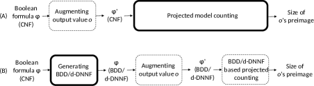
Figure 1: (A): Compute-on-Demand, (B): Construct-in-Advance.

A box surrounded by bold lines represents a heavy-weighted process, which requires much computing resource. The main difference between (A) and (B) is the relative position of the heavy-weighted process, i.e., whether (A) to put the process after augmenting an observed output and then run the process each time we need (on demand) to compute dynamic leakage, or (B) to put the process before augmenting an observed output (in advance) so that we should run the process only once for one program. In CoD, the heavy-weighted process is a projected model counting, for which off-the-shelf tools such as SharpCDCL [29], DSharp-p [24] and GPMC [25] can be used. In CiA, the heavy-weighted process is the one that generates BDD [20] or d-DNNF [11], which are data structures to represent Boolean formulas. Generally, it takes time to generate BDD or d-DNNF but counting all solutions (models) by using them is easy. CiA takes the full advantage of this characteristic. Consider again Example 1 above. The set of all feasible pairs of ($source$, $output$) is $2^{32}$. Even for such a simple program, using BDD or d-DNNF to store all those pairs is quite daunting in terms of both memory space and speed. Therefore, for programs with simple structure but a large number of input and output pairs, CoD works better than CiA. On the other hand, CiA is preferable to CoD when quantifying dynamic leakage is required many times on the same program. However, CoD or CiA alone is not a solution to the problem of scalability.

In this paper, we introduce two compositional methods for computing dynamic leakage inspired by the work of Kawamoto et al. [14] on the compositionality of static leakage. One is to utilize the sequential structure of a given program $P=P_{1};P_{2}$. We first analyze $P_{2}$ and then compute the leakage of $P$ by analyzing $P_{1}$ based on the result on $P_{2}$. For the sequential composition, beside the benign yet time-consuming exact counting based on Breadth-First-Search (BFS), we also investigate an approximated approach. For upper bound of the count, we leverage the results on each sub-program by Max#SAT in [12]. For lower bound of the count, we simply use Depth-First-Search (DFS) with timeout, i.e., DFS will stop when the execution time exceeds the predetermined timeout.

The other method we propose is based on the decomposition of the value domain of a program. For example, we divide the input domain as $I=I_{1}\cup I_{2}$ and the output domain as $O=O_{1}\cup O_{2}$ of a program $P(I,O)$, compute the leakages for $P(I_{i},O_{j})$ for $i=1,2$ and $j=1,2$, and then compute the leakage of the whole program $P(I,O)$ from them. This value domain based decomposition has two merits. First, it is flexible yet simple to adjust the components. Secondly, the exact dynamic leakage of the composed program can be simply derived by taking the sum of those of its components. Despite the number of components can be large, this approach is promising with parallel computing.

In summary, the contributions of this research are four-fold:

• We propose a compositional method for dynamic leakage computation based on the sequential structure inside a given program and the composability of the leakage of the whole program from those of subprograms.

• We propose another compositional method based on value domains, which is suitable for parallel computing.

• We propose an approximated approach where we upper bound the count using Max#SAT problem and lower bound the count by DFS with predetermined timeout.

• We prototype a tool that can do parallel computation based on value domain decomposition and both exact counting and approximated counting for the sequential composition. By using the tool, we investigate feasibility and advantages of the proposed compositional methods for computing dynamic leakage of several examples.

Related work Definitions of QIF: Smith [19] gives a comprehensive summary on entropy-based QIF, such as Shannon entropy, guessing entropy and min entropy and compares them in various scenarios. Clarkson et al. [9], on the other hand, include attacker’s belief into their model. Alvim et al. introduce gain function to generalize information leakage by separating the probability distribution and the impact of individual information. Computational Complexity: Yasuoka and Terauchi [22] prove complexity on computing QIF, including $PP$-hardness of precisely quantifying QIF for loop-free Boolean programs. Chadha and Ummels [6] show that the QIF bounding problem of recursive Boolean programs is EXPTIME-complete. Precise Calculation: In [15], Klebanov et al. reduce QIF calculation to #SAT problem projected on a specific set of variables. On the other hand, Phan et al. [18] reduce QIF calculation to $\sharp$SMT problem to leverage existing SMT (satisfiability modulo theory) solvers. Recently, Val et al. [21] reported a SAT-based method that can scale to programs of 10,000 lines of code. Approximated Calculation: Approximation is a reasonable alternative for scalability. Köpf and Rybalchenko [16] propose approximated QIF computation by sandwiching the precise QIF with lower and upper bounds using randomization and abstraction, respectively, with a provable confidence. LeakWatch of Chothia et al. [7], also give approximation with provable confidence by executing a program multiple times. Its descendant called HyLeak [5] combines the randomization strategy of its ancestor with precise analysis. Biondi et al. [4] utilize ApproxMC2, which provides approximation on the number of models of a Boolean formula in CNF by Markov Chain Monte Carlo method. Composition of QIF: Another attempt to the scalability is to break the system down into smaller fragments. In [14], Kawamoto et al. introduce two parallel compositions: with distinct inputs and with shared inputs, and give theoretical bounds on the leakage of the main program using those of the constituted sub-programs. Though our research was motivated by [14], we focus on a sequential structure of a target program and a decomposition of the value domain of the program while [14] uses a parallel structure of the target. Dynamic Leakage: Bielova ([3]) discusses the importance of dynamic leakage and argues that any well-known QIF notion is not appropriate as a notion for dynamic leakage. Recently, we proposed two notions for dynamic leakage, $\mbox{QIF}_{1}$ and $\mbox{QIF}_{2}$ and give some results on computational complexity as well as a quantifying method based on model counting [8].

The rest of the paper is organized as follows. We will review the definition of dynamic leakage and assume our program model in Section 2. Section 3 is dedicated to a method for computing dynamic leakage based on the sequential composition and also propose approximation methods. Section 4 proposes a parallel computation method based on value domain decomposition. Section 5 evaluates the proposed compositional methods including the comparison of CiA vs. CoD and exact vs. approximated computation based on the experimental results. Then the paper is concluded in Section 6.

2 Preliminaries

2.1 Dynamic leakage

The standard notion for static quantitative information flow (QIF) is defined as the mutual information between random variables $S$ for secret input and $O$ for observable output:

$$\mbox{QIF}=H(S)-H(S|O)$$ (1)

where $H(S)$ is the entropy of $S$ and $H(S|O)$ is the expected value of $H(S|o)$, which is the conditional entropy of $S$ when observing an output $o$. Shannon entropy and min-entropy are often used as the definition of entropy, and in either case, $H(S)-H(S|O)\geq 0$ always holds by the definition.

In [3], the author discusses the appropriateness of the existing measures for dynamic QIF and points out their drawbacks, especially, each of these measures may become negative. Hereafter, let ${\cal S}$ and ${\cal O}$ denote the finite sets of input values and output values, respectively.

Let $P$ be a program with secret input variable $S$ and observable output variable $O$. For notational convenience, we identify the names of program variables with the corresponding random variables. Throughout the paper, we assume that a program always terminates. The syntax and semantics of programs assumed in this paper will be given in the next section. For $s\in{\cal S}$ and $o\in{\cal O}$, let $p_{SO}(s,o)$, $p_{O|S}(o|s)$, $p_{S|O}(s|o)$, $p_{S}(s)$, $p_{O}(o)$ denote the joint probability of $s\in{\cal S}$ and $o\in{\cal O}$, the conditional probability of $o\in{\cal O}$ given $s\in{\cal S}$ (the likelihood), the conditional probability of $s\in{\cal S}$ given $o\in{\cal O}$ (the posterior probability), the marginal probability of $s\in{\cal S}$ (the prior probability) and the marginal probability of $o\in{\cal O}$, respectively. We often omit the subscripts as $p(s,o)$ and $p(o|s)$ if they are clear from the context. By definition, $p(s,o)=p(s|o)p(o)=p(o|s)p(s)$, $p(o)=\sum_{s\in{\cal S}}p(s,o)$, $p(s)=\sum_{o\in{\cal O}}p(s,o)$.

We assume that (the source code of) $P$ and the prior probability $p(s)$ ($s\in{\cal S}$) are known to an attacker. For $o\in{\cal O}$, let $\mbox{pre}_{P}(o)=\{s\in{\cal S}\mid p(s|o)>0\}$, which is called the preimage of $o$ (by the program $P$).

Considering the discussions in the literature, we define new notions for dynamic QIF that satisfy the following requirements [8]:

1. Dynamic QIF should be always non-negative because an attacker obtains some information (although sometimes very small or even zero) when he observes an output of the program.

2. It is desirable that dynamic QIF is independent of a secret input $s\in{\cal S}$. Otherwise, the controller of the system may change the behavior for protection based on the estimated amount of the leakage that depends on $s$, which may be a side channel for an attacker.

3. The new notion should be compatible with the existing notions when we restrict ourselves to special cases such as deterministic programs, uniformly distributed inputs, and taking the expected value.

The first notion is the self-information of the secret inputs consistent with an observed output $o\in{\cal O}$. Equivalently, the attacker can narrow down the possible secret inputs after observing $o$ to the preimage of $o$ by the program. We consider the self-information of $s\in\mathcal{S}$ after the observation as the probability of $s$ divided by the sum of the probabilities of the inputs in the preimage of $o$ (see the upper part of Fig. 2).

$$\mbox{QIF}_{1}^{P}(o) = -\log(\sum_{s^{\prime}\in\mbox{pre}_{P}(o)}p(s^{\prime})).$$ (2)

Figure 2: $\mbox{QIF}_{1}$ (the upper) and $\mbox{QIF}_{2}$ (the lower)

The second notion is the self-information of the joint events $s^{\prime}\in{\cal S}$ and an observed output $o\in{\cal O}$ (see the lower part of Fig. 2). This is equal to the the self-information of $o$.

$$\mbox{QIF}_{2}^{P}(o)=-\log(\sum_{s^{\prime}\in{\cal S}}p(s^{\prime},o))=-\log p(o)=-\log p(s,o)+\log p(s|o).$$ (3)

Both notions are defined by considering how much possible secret input values are reduced by observing an output. We propose two notions because there is a trade-off between the easiness of calculation and the appropriateness [8].

Theorem 2.1 ([8]).

If a program $P$ is deterministic, for every $o\in{\cal O}$ and $s\in{\cal S}$,

$$\mbox{QIF}_{1}^{P}(o)=\mbox{QIF}_{2}^{P}(o)=-\log p(o).$$

If input values are uniformly distributed, $\mbox{QIF}_{1}^{P}(o)=$ $\log\frac{|{\cal S}|}{|\mbox{pre}_{P}(o)|}$ for every $o\in{\cal O}$. ∎

2.2 Program model

We assume probabilistic programs where every variable stores a natural number and the syntactical constructs are assignment to a variable, conditional, probabilistic choice, while loop and concatenation:

$$b ::= \bot\mid\top\mid\neg b\mid b\vee b\mid e<e$$

$$e ::= X\mid n\mid e+e$$

$$c ::= \mbox{skip}\mid X\leftarrow e\mid\mbox{if }b\mbox{ then }c\mbox{ else }c\mbox{ end}$$

$$\mid c~{}_{r}[]_{1-r}~{}c\mid\mbox{while }b\mbox{ do }c\mbox{ end}\mid c;c$$

where $<,X,n,+$ stand for a binary relation on natural numbers, a program variable, a constant natural number and a binary operation on natural numbers, respectively, and $r$ is a constant rational number representing the branching probability for a choice command where $0\leq r\leq 1$. In the above BNFs, objects derived from the syntactical categories $b$, $e$ and $c$ are called conditions, expressions and commands, respectively. A command $X\leftarrow e$ assigns the value of expression $e$ to variable $X$. A command $c_{1~{}r}[]_{1-r}~{}c_{2}$ means that the program chooses $c_{1}$ with probability $r$ and $c_{2}$ with probability $1-r$. Note that this is the only probabilistic command. The semantics of the other constructs are defined in the usual way.

A program $P$ has the following syntax:

$$P ::= \mbox{in }\vec{S};\mbox{ out }\vec{O};\mbox{ local }\vec{Z};c\mid P;P$$

where $\vec{S},\vec{O},\vec{Z}$ are sequences of variables which are disjoint from one another. A program is required to satisfy the following constraints on variables. We first define $In(P),Out(P),Local(P)$ for a program $P$ as follows.

• If $P=\mbox{in }\vec{S};\mbox{ out }\vec{O};\mbox{ local }\vec{Z};c$, we define $In(P)=\{V\mid V\mbox{ appears in }\vec{S}\}$, $Out(P)=\{V\mid V\mbox{ appears in }\vec{O}\}$ and $Local(P)=\{V\mid V\mbox{ appears in }\vec{Z}\}$. In this case, we say $P$ is a simple program. We require that no varible in $In(P)$ appears in the left-hand side of an assignment command in $P$, i.e., any input variable is not updated.

• If $P=P_{1};P_{2}$, we define $In(P)=In(P_{1})$, $Out(P)=Out(P_{2})$ where we require that $In(P_{2})=Out(P_{1})$ holds. We also define $Local(P)=Local(P_{1})\cup Local(P_{2})\cup Out(P_{1})$.

A program $P$ is also written as $P(S,O)$ where $S$ and $O$ are enumerations of $In(P)$ and $Out(P)$, respectively. A program $P_{1};P_{2}$ represents the sequential composition of $P_{1}$ and $P_{2}$. Note that the semantics of $P_{1};P_{2}$ is defined in the same way as that of the concatenation of commands $c_{1};c_{2}$ except that the input and output variables are not always shared by $P_{1}$ and $P_{2}$ in the sequential composition. If a program does not have a probabilistic choice, it is deterministic.

3 Sequential composition

This section proposes a method of computing both exact and approximated dynamic leakage by using sequential composition. While the formula in exact calculation can be used for both probabilistic and deterministic programs, we consider only deterministic programs with uniformly distributed input.

3.1 Exact calculation

For a program $P(S,O)$, an input value $s\in{\cal S}$ and a subset ${\cal S}^{\prime}$ of input values, let

$$\mbox{post}_{P}(s) = \{o\mid p(o|s)>0\},$$

$$\mbox{post}_{P}({\cal S}^{\prime}) = \bigcup_{s\in{\cal S}^{\prime}}\mbox{post}_{P}(s).$$

If $P$ is deterministic and $\mbox{post}_{P}(s)=\{o\}$, we write $\mbox{post}_{P}(s)=o$.

Let $P=P_{1};P_{2}$ be a program. We assume that $In(P_{1}),Out(P_{1}),In(P_{2}),Out(P_{2})$ are all singleton sets for simplicity. This assumption does not lose generality; for example, if $In(P_{1})$ contains more than one variables, we instead introduce a new input variable that stores the tuple consisting of a value of each variable in $In(P_{1})$. Let $In(P)=In(P_{1})=\{S\}$, $Out(P_{1})=In(P_{2})=\{T\}$, $Out(P)=Out(P_{2})=\{O\}$, and let ${\cal S},{\cal T},{\cal O}$ be the corresponding sets of values, respectively. For a given $o\in{\cal O}$, $\mbox{pre}_{P}(o)$ and $p(o)$, which are needed to compute $\mbox{QIF}_{1}^{P}(o)$ and $\mbox{QIF}_{2}^{P}(o)$, (see (2) and (3)) can be represented in terms of those of $P_{1}$ and $P_{2}$ as follows.

$$\mbox{pre}_{P}(o) = \bigcup_{t\in(\mbox{pre}_{P_{2}}(o)\cap\mbox{post}_{P_{1}}({\cal S}))}\mbox{pre}_{P_{1}}(t),$$ (4)

$$p(o) = \sum_{s\in{\cal S},t\in{\cal T}}p(s)p_{1}(t|s)p_{2}(o|t).$$ (5)

If $p(s)$ is given, we can compute (4) by enumerating the sets $\cal T$ and $\mbox{pre}_{P_{1}}(t)$ for $t\in(\mbox{pre}_{P_{2}}(o)\cap\mbox{post}_{P_{1}}({\cal S}))$ and also for (5). This approach can easily be generalized to the sequential composition of more than two programs, in which the enumeration is proceeded in Breadth-First-Search fashion. However, in this approach, search space will often explode rapidly and lose the advantage of composition. Therefore we come up with approximation, which is explained in the next subsection, as an alternative.

3.2 Approximation

Let us assume that $P(S,O)$ is deterministic and $S$ is uniformly distributed. In this subsection, we will derive both upper-bound and lower-bound of $|\mbox{pre}_{P}(o)|$ which provides lower-bound and upper-bound of $\mbox{QIF}_{1}^{P}(o)=\mbox{QIF}_{2}^{P}(o)$ respectively. In general, our method can be applied to the sequential composition of more than two sub-programs.

3.2.1 Lower bound

To infer a lower bound of $|\mbox{pre}_{P}(o)|$, we leverage Depth-First-Search (DFS) with a predefined timeout such that the algorithm will stop when the execution time exceeds the timeout and output the current result as the lower bound. The method is illustrated in Algorithm 1. The problem is defined as: given a program $P=P_{1};P_{2};\cdots;P_{n}$, an observable output $o$ of the last sub-program $P_{n}$ and a predetermined $timeout$, derive a lower bound of $|\mbox{pre}_{P}(o)|$ by those $n$ sub-programs.

Algorithm 1 LowerBound($P_{1},\cdots,P_{n},o$, timeout)

1:$Pre[2..n]\leftarrow empty$

2:$Stack\leftarrow empty$

3:$level\leftarrow n$

4:$acc\_count\leftarrow 0$

5:Push($Stack,o$)

6:$Pre[n]\leftarrow EnumeratePre(P_{n},o)$

7:while not $Stack.empty$ and $execution\_time<timeout$ do

8:     if $level=1$ then

9:         $acc\_count\leftarrow acc\_count+$ CountPre($P_{1},Stack.top$)

10:         $level\leftarrow level+1$

11:         Pop($Stack$)

12:     else

13:         $v\leftarrow$ PickNotSelected($Pre[level]$)

14:         if $v=AllSelected$ then

15:              $level\leftarrow level+1$

16:              Pop($Stack$)

17:         else

18:              Push($Stack,v$)

19:              $level\leftarrow level-1$

20:              if $level>1$ then

21:                  $Pre[level]\leftarrow EnumeratePre(P_{level},v)$                             

22:return $acc\_count$

In Algorithm 1, CountPre(Q, o) counts $|\mbox{pre}_{Q}(o)|$, PickNotSelected(Pre[i]) select an element of $Pre[i]$ that has not been traversed yet or returns AllSelected if there is no such element, and EnumeratePre($P_{i},v$) lists all elements in $\mbox{pre}_{P_{i}}(v)$. $Pre[i]$ stores $\mbox{pre}_{P_{i}}(o_{i})$ for some $o_{i}$. For $P_{1}$, it is not necessary to store its preimage because we need only the size of the preimage. Lines 1 to 5 are for initialization. Line 6 enumerates $\mbox{pre}_{P_{n}}(o)$. Lines 7 to 21 constitute the main loop of the algorithm, which is stopped either when the counting is done or when time is up. When $level=1$, lines 8 to 11 are executed and $CountPre$ will return $\mbox{pre}_{P_{1}}(Stack.top)$ in which $Stack.top$ is the input of $P_{2}$ that leads to output $o$ of $P_{n}$, then back-propagate; lines 13 to 16 check if all elements in the preimage set of the current level is already considered and if so, back-propagate, otherwise push the next element onto the top of $Stack$ and go to the next level.

Theorem 3.1.

In Algorithm 1, if $P_{1},\cdots,P_{n}$ are deterministic, $acc\_count$, which is returned at line 22, is a lower bound of the preimage size of $o$ by $P_{1},\cdots,P_{n}$. ∎

3.2.2 Upper bound

For an upper bound of $|\mbox{pre}_{P}(o)|$ we use Max#SAT problem [12], which is defined as follows.

Definition 3.1.

Given a propositional formula $\varphi(X,Y,Z)$ over sets of variables $X$, $Y$ and $Z$, the Max#SAT problem is to determine $max_{X}\#Y.\exists Z.\varphi(X,Y,Z)$.

Let us consider a program $Q$, $In(Q)$, $Out(Q)$ and $Local(Q)$ as $\varphi$, $Y$, $X$ and $Z$ respectively. Then, the solution $X$ to the Max#SAT problem can be interpreted as the output value which has the biggest size of its preimage set. In other words, $|max_{X}\#Y.\exists Z.\varphi(X,Y,Z)|$ is an upper bound of $\mbox{pre}_{Q}$ over all feasible outputs. Therefore, the product of those upper bounds of $|\mbox{pre}_{P_{i}}|$ over all $i$($1\leq i\leq n$) is obviously an upper bound of $|\mbox{pre}_{P}|$. Algorithm 2 computes this upper bound where $CountPre(P_{n},o)$ returns the size of the preimage of $o$ by $P_{n}$; $MaxCount(P_{i})$ computes the answer to the Max#SAT problem for program $P_{i}$. We used the tool developed by the authors of [12], which produces estimated bounds of Max#SAT with tunable confidence and precision. As explained in [12], the tool samples output values of $k$-fold self-composition of the original program. The greater $k$ is, the more precise the estimation is, but also the more complicated the calculation of each sampling is. Note that $MaxCount(P_{i})$ can be computed in advance only once.

Algorithm 2 UpperBound($P_{1},\cdots,P_{n},o$)

1:$Result\leftarrow CountPre(P_{n},o)$

2:for $i\leftarrow 1$ to $n$ do

3:     $Result\leftarrow Result*MaxCount(P_{i})$

4:return $Result$

Theorem 3.2.

In Algorithm 2, if $P_{1},\cdots,P_{n}$ are deterministic, $Result$, which is returned at line 4, is an upper bound of the preimage size of $o$ by $P_{1},\cdots,P_{n}$. ∎

4 Value domain decomposition

Another effective method for computing the dynamic leakage in a compositional way is to decompose the sets of input values and output values into several subsets, compute the leakage for the subprograms restricted to those subsets, and compose the results to obtain the leakage of the whole program. The difference between the parallel composition in [14] and the proposed method is that in the former case, a program under analysis itself is divided into two subprograms that run in parallel, and in the latter case, the computation of dynamic leakage is conducted in parallel by decomposing the sets of input and output values.

Let $P(S,O)$ be a program. Assume that the sets of input values and output values, ${\cal S}$ and ${\cal O}$, are decomposed into mutually disjoint subsets as

$${\cal S} = {\cal S}_{1}\uplus\cdots\uplus{\cal S}_{k},$$

$${\cal O} = {\cal O}_{1}\uplus\cdots\uplus{\cal O}_{l}.$$

For $1\leq i\leq k$ and $1\leq j\leq l$, let $P_{ij}$ be the program obtained from $P$ by restricting the set of input values to ${\cal S}_{i}$ and the set of output values to ${\cal O}_{j}$ where if the output value $o$ of $P$ for an input value $s\in{\cal S}_{i}$ does not belong to ${\cal O}_{j}$, the output value of $P_{ij}$ for input $s$ is undefined.

By definition, for a given $o\in{\cal O}_{j}$,

$$\mbox{pre}_{P}(o)=\bigcup_{1\leq i\leq k}\mbox{pre}_{P_{i,j}}(o).$$ (*)

By (2) and (3), we can compute $\mbox{QIF}_{1}$ and $\mbox{QIF}_{2}$ in a compositional way.

By Theorem 2.1, if $P$ is deterministic and the prior probability of $S$ is uniformly distributed, what we have to compute is $|\mbox{pre}_{P}(o)|$, which can be obtained by summing up each $|\mbox{pre}_{P_{i,j}}(o)|$ by (* ‣ 4).

$$|\mbox{pre}_{P}(o)| = \sum_{1\leq i\leq k}|\mbox{pre}_{P_{i,j}}(o)|.$$

5 Experiments

This section will investigate answers for the following questions: (1) Is CiA always better than CoD or vice versa? (2) How can parallel computation based on the value domain decomposition improve the performance? (3) How does approximation in the sequential composition work in terms of precision and speed? We will examine those questions through a few examples.

5.1 Setting up

The experiments were conducted on Intel(R) Xeon(R) CPU ES-1620 v3 @ 3.5GHz x 8 (4 cores x 2 threads), 32GB RAM, CentOS Linux 7. For parallel computation, we use OpenMP [10] library. At the very first phase to transform C programs into CNFs, we leveraged the well-known CBMC[23]. For the construction of a BDD from a CNF and the model counting and enumeration of the constructed BDD, we use an off-the-shell tool PC2BDD [27]. We use PC2DDNNF [28] for the d-DNNF counterpart. Both of the tools are developed by one of the authors in another project. Besides, as an ordering of Boolean variables of a CNF greatly affects the BDD generation performance, we utilize FORCE [1] to optimize the ordering before transforming a CNF into a BDD. We use MaxCount [26] for estimating the answer of Max#SAT problem. We implemented a tool for Algorithms 1 and 2 as well as the exact count in sequential compositions in Java.

5.2 The grade protocol

This benchmark is taken from [17]. By this experiment, we investigated answers for questions (1) and (2) mentioned at the beginning of this section. This benchmark sums up (then takes the average of) the grades of a group of students without revealing the grade of each student. We used the benchmark with 4 students and 5 grades, and all variables are of 16 bits. For model counting, we suppose the observed output (the sum of students’ grades) to be 1, and hence the number of models is 4. GPMC [25], one of the fastest tools for quantifying dynamic leakage as shown in [8], was chosen as the representative tool for CoD approach. We manually decompose the original program into 4, 8 and 32 sub-programs by adding constraints on input and output of the program based on the value domain decomposition (the set of output values is divided into 2 and the set of input values is divided into 2, 4 or 16). Table 1 is divided into sub-divisions corresponding to specific tasks: BDD construction, d-DNNF construction and model counting based on different approaches. In each sub-division, the bold number represents the shortest execution time in each column (i.e., the same number of decomposed sub-programs, but different numbers of threads) and the underlined one represents the best in that sub-division. ‘$-$’ represents cases when the number of threads is greater than the number of sub-programs, which are obviously meaningless to do experiments.

		$n=32$	$n=8$	$n=4$	$n=1$
BDD Construction	$t=32$	218.53s	$-$	$-$	$-$
	$t=16$	$222.27s$	$-$	$-$	$-$
	$t=8$	$237.54s$	137.74s	$-$	$-$
	$t=4$	$254.88s$	$144.55s$	155.90s	$-$
	$t=2$	$376.21s$	$233.34s$	$214.65s$	$-$
	$t=1$	$736.74s$	$450.85s$	$391.99s$	$\textbf{243.85}s$
d-DNNF Construction	$t=32$	$93.17s$	$-$	$-$	$-$
	$t=16$	91.49s	$-$	$-$	$-$
	$t=8$	$107.31s$	123.48s	$-$	$-$
	$t=4$	$141.27s$	$147.79s$	175.34s	$-$
	$t=2$	$215.92s$	$226.93s$	$247.45s$	$-$
	$t=1$	$398.99s$	$391.67s$	$457.38s$	304.88s
Model Counting (CiA - BDD based)	$t=32$	0.21s	$-$	$-$	$-$
	$t=16$	$0.22s$	$-$	$-$	$-$
	$t=8$	$0.25s$	0.13s	$-$	$-$
	$t=4$	$0.30s$	$0.16s$	0.16s	$-$
	$t=2$	$0.65s$	$0.31s$	$0.24s$	$-$
	$t=1$	$0.86s$	$0.36s$	$0.31s$	0.30s
Model Counting (CiA - d-DNNF based)	$t=32$	0.05s	$-$	$-$	$-$
	$t=16$	0.05s	$-$	$-$	$-$
	$t=8$	0.05s	0.01s	$-$	$-$
	$t=4$	$0.07s$	0.01s	0.01s	$-$
	$t=2$	$0.12s$	$0.02s$	$0.02s$	$-$
	$t=1$	$0.18s$	$0.04s$	$0.03s$	0.25s
Model Counting (CoD - using GPMC)	$t=1$	$-$	$-$	$-$	44.69s

Table 1: Excecution time for the construction of data structures and model counting of different approaches. $n$: number of sub-programs decomposed from the original program; $t$: number of threads specified by num_thread compiling directive of OpenMP.

Let us keep in mind that $n=1$ means non-decomposition, $t=1$ means a serial execution and the number of physical CPUs of the hardware is 8. From Table 1, we can infer the following conclusion:

• In general, increasing the number of threads (up to the number of sub-programs) does improve the execution time in both the construction of data structures and the model counting.

• When the number of sub-programs is close to the number of physical CPUs (8), the execution time is among the best if not the best.

• In this example, CiA shows a huge improvement over CoD, which is more than 4000 times (0.01s vs. 44.69s) with the best tuning of the former. Of course, CiA takes time in constructing data structures BDD or d-DNNF.

The performance with d-DNNF is better than that with BDD in this example, but this seems due to the implementation of the tools.

5.3 Bit shuffle and Population count

population_count is the 16-bit version of the benchmark of the same name given in [17]. In this experiment, the original program is decomposed into three sub-programs in such a way that each sub-program performs one bit operation of the original. Inspired by population_count, we created the benchmark bit_shuffle, which consists of two steps: firstly it counts the number of bit-ones in a given secret number (by population_count), then it shuffles those bits to produce an output value. Though in Section 3, we suppose programs to be deterministic, when it comes to calculate $\mbox{QIF}_{1}$, the theory part works for probabilistic programs as well. Hence, even bit_shuffle is probabilistic, conducting experiments on it is still valid.

This original program is divided into two sub-programs corresponding to the two steps. All the original programs and the decomposed sub-programs are provided in appendix 0.A. As shown in Table 2, the construction time of BDD and d-DNNF for bit_shuffle was improved significantly (more than 100 times for BDD, 8 times for d-DNNF) by the decomposition while the improvement of population_count was not large. This is because in the former case two sub-programs are connected at a bottle-neck point, i.e., given a certain output, its preimage by the second program always has exactly one element, which is the number of bit-ones of that output, while in the latter case there is no such bottle-neck point. Besides, parallel computing is available for the decomposed sub-programs and the result is a little bit better. Probably, as the number of sub-programs increases, the effect of parallel computing would be larger.

For model counting, we let an output value be 3 (the number of models is 13110) for bit_shuffle and 7 (the number of models is 11440) for population_count. Table 3 presents the execution times for model counting where the underlined numbers are the exact counts, the bold excution times are the best results among approaches for the exact count of each benchmark and the italic data are of approximated calculations. The execution times for the lower bounds are predetermined timeouts, which were designed to be 1/2, 1/5 and 1/10 of the time needed by the exact count, followed by the time by CoD. In bit_shuffle benchmark, lower bounds based on d-DNNF were not improved (all are zero) even the timeout was increased. This happened because an intermediate result of counting for one d-DNNF is unknown until the counting completes while this benchmark contains only two sub-programs and the size of the preimage by the second sub-program is always one (i.e., the number of times to count d-DNNFs is only two, one for the first sub-program and one for the second one).

		non-decompose	decompose (serial)	decompose (parallel)
BDD Construction	bit_shuffle	$>$1 hour	33.90s	33.46s
	population_count	0.48s	0.66s	0.40s
d-DNNF Construction	bit_shuffle	424.64s	50.28s	48.39s
	population_count	1.19s	0.71s	0.69s

Table 2: BDD and d-DNNF construction time for different approaches.

			bit_shuffle		population_count
CoD using GPMC			0.49s	13110	0.09s	11440
CiA-BDD based	Exact count		1.47s	13110	10.98s	11440
	Approximation	Lower bound	0.75s	6243	5.5s	5776
			0.30s	1918	2.2s	888
			0.15s	574	1.1s	312
			0.49s	3713	0.09s	0
		Upper bound	0.02s	14025	0.07s	5898240
CiA-d-DNNF based	Exact count		0.27s	13110	3.50s	11440
	Approximation	Lower bound	0.13s	0	1.75s	4712
			0.05s	0	0.70s	1314
			0.03s	0	0.35s	52
			0.49s	13110	0.09s	0
		Upper bound	0.07s	14025	0.13s	5898240

Table 3: Model counting: execution time and the changing of approximation precision.

From the experimental results, we obtain the following observations.

• In the previous section (grade protocol) CiA did much better than CoD while in this section, especially for population_count benchmark, CoD using GPMC offered a huge improvement over CiA. So the answer for question (1) is ‘No’.

• While the precision of the upper bounds was not so good, their execution times were small. The precision could be improved by tuning the decomposition. So this result could be a hint to a research on how to make a good decomposition to benefit the upper bound approximation.

• As expected, the lower bounds were improved as the timeout was lengthened. Note that a lower bound of the model count corresponds to an upper bound of $\mbox{QIF}_{1}$. Therefore, if we set a threshold for the leakage of a program, we only need to know whether the lower bound of the counting exceedes the constant corresponding to the threshold, and if so, we can terminate the analysis but still be sure about the safety of the program.

6 Conclusion

In this paper, we focused on the efficient computation of dynamic leakage of a program and considered two approaches Compute-on-Demand (CoD) and Construct-in-Advance (CiA). Then, we proposed two compositional methods, namely, computation along with the sequential structure of the program and parallel computation based on value domain decomposition. In the first method, we also proposed approximations that give both lower bound and upper bound of model counting. Our experimental result showed that: (1) both CiA and CoD are important because sometimes the former works better and the other times does the latter; (2) Parallel computation based on value domain decomposition works well generally; and (3) the precision of upper bound depends on the way of decomposition while that of lower bound depends on the preset timeout. However, all decomposition in the experiments were done manually and finding a systematical way of deciding a good decomposition is left as future work. Both BDD and d-DNNF have many applications other than computing dynamic leakage, but there is still a bottle neck at generating them from an object to be analyzed. One of the approaches in this paper composition based on value domains can be a hint to speed up that process.

Appendix 0.A Benchmarks

0.A.1 Grade protocol

0.A.1.1 Original program

⬇

1typedef unsigned int size_t;

2size_t nondet_int();

3int main(void){

4size_t S = 4, G=5; //number of students, number of grades.

5size_t n, output, sum = 0, i=0, j=0, c=0;

6size_t numbers[S], announcements[S], h[S];

7

8n = ((G-1)*S)+1;

9for (c = 0; c < S; c++) { h[c] = nondet_int() % G;}

10for (c = 0; c < S; c++) { numbers[c] = nondet_int() % n;}

11while (i<S) {

12 j=0;

13 while (j<G) {

14 if (h[i]==j)

15 announcements[i]=j+numbers[i]-numbers[(i+1)%S];

16 j=j+1;

17 }

18 i=i+1;

19}

20

21//computing the sum, producing the output and terminating

22for (c = 0; c < S; c++) { sum += announcements[c]; }

23output = sum % n;

24

25assert(0);

26return 0;

27}

Listing 1: grade.c

0.A.1.2 One of sub-programs in 32-parts decomposition

⬇

1typedef unsigned int size_t;

2size_t nondet_int();

3int main(void){

4size_t S = 4, G=5; //number of students, number of grades.

5size_t n, output, sum = 0, i=0, j=0, c=0;

6size_t numbers[S], announcements[S], h[S];

7

8n = ((G-1)*S)+1;

9for (c = 0; c < S; c++) { h[c] = nondet_int() % G;}

10__CPROVER_assume (h[0]>=0 && h[0]<3);

11__CPROVER_assume (h[1]>=0 && h[1]<3);

12__CPROVER_assume (h[2]>=0 && h[2]<3);

13__CPROVER_assume (h[3]>=0 && h[3]<3);

14for (c = 0; c < S; c++) { numbers[c] = nondet_int() % n;}

15while (i<S) {

16j=0;

17while (j<G) {

18if (h[i]==j)

19announcements[i]=j+numbers[i]-numbers[(i+1)%S];

20j=j+1;

21}

22i=i+1;

23}

24

25//computing the sum, producing the output and terminating

26for (c = 0; c < S; c++) { sum += announcements[c]; }

27output = sum % n;

28

29assert(output < 0 || output > 8);

30return 0;

31}

Listing 2: grade_32_01.c

0.A.2 Bit Shuffle

0.A.2.1 Original program

⬇

1unsigned short int nondet_int();

2int main(void){

3unsigned short int s, s0, o=0, count;

4s0=s;

5s=(s&0x5555)+((s>>1)&0x5555);

6s=(s&0x3333)+((s>>2)&0x3333);

7s=(s&0x0f0f)+((s>>4)&0x0f0f);

8count=(s+(s>>8))&0xff;

9count=count%6;

10unsigned short int bit_arr[16];

11unsigned short int indices[16];

12

13// initialize

14for (unsigned int i=0; i<16; i++){

15bit_arr[i]=0;

16indices[i]=i;

17}

18

19// shuffle

20for (unsigned int i=16; i>16-count; i–) {

21unsigned int j = nondet_int()%i;

22bit_arr[indices[j]]=1;

23unsigned int temp=indices[j];

24indices[j]=indices[i-1];

25indices[i-1]=temp;

26}

27

28// generate result

29for (unsigned int i=0; i<16; i++) {

30if (bit_arr[i] == 1) o += 1 << (16 - i - 1);

31}

32return 0;

33}

Listing 3: bit_shuffle.c

0.A.2.2 Sub-programs

⬇

1typedef unsigned short int g_type;

2g_type nondet_int();

3int main(void) {

4g_type s, s0;

5g_type count;

6

7s0 = s;

8s = (s & 0x5555) + ((s >> 1) & 0x5555);

9s = (s & 0x3333) + ((s >> 2) & 0x3333);

10s = (s & 0x0f0f) + ((s >> 4) & 0x0f0f);

11count = (s + (s>>8)) & 0xff;

12count = count % 6;

13

14assert(0);

15return 0;

16}

Listing 4: bit_shuffle_2_1.c

⬇

1typedef unsigned short int g_type;

2g_type nondet_int();

3int main(void) {

4g_type o, count;

5

6count = count % 6;

7unsigned short int bit_arr[16], indices[16];

8

9// initialize

10for (unsigned int i=0; i<16; i++) {

11 bit_arr[i] = 0;

12 indices[i] = i;

13}

14

15// shuffle

16for (unsigned int i=16; i>16-count; i–) {

17 unsigned int j = nondet_int() % i;

18 bit_arr[indices[j]] = 1;

19 // swap

20 unsigned int temp = indices[j];

21 indices[j] = indices[i-1];

22 indices[i-1] = temp;

23}

24

25// generate result

26o = 0;

27

28for (unsigned int i=0; i<16; i++) { if (bit_arr[i] == 1) o += 1 << (16 - i - 1);}

29assert(0);

30return 0;

31}

Listing 5: bit_shuffle_2_2.c

0.A.3 Population Count

0.A.3.1 Original programs

⬇

1int main(void) {

2unsigned short int S0, S, Output;

3S0 = S;

4S = (S & 0x5555) + ((S >> 1) & 0x5555);

5S = (S & 0x3333) + ((S >> 2) & 0x3333);

6S = (S & 0x0f0f) + ((S >> 4) & 0x0f0f);

7Output = (S + (S>>8)) & 0xff;

8assert(0);

9return Output;

10}

Listing 6: population_count.c

0.A.3.2 Sub-programs

⬇

1int main(void){

2unsigned short int S0, S;

3S0 = S;

4S = (S & 0x5555) + ((S >> 1) & 0x5555);

5assert(0);

6return S;

7}

Listing 7: population_count_3_1.c

⬇

1int main(void){

2unsigned short int S0, S;

3S0 = S;

4S = (S & 0x3333) + ((S >> 2) & 0x3333);

5assert(0);

6return S;

7}

Listing 8: population_count_3_2.c

⬇

1int main(void){

2unsigned short int S0, S, Output;

3S0 = S;

4S = (S & 0x0f0f) + ((S >> 4) & 0x0f0f);

5Output = (S + (S>>8)) & 0xff;

6assert(0);

7return Output;

8}

Listing 9: population_count_3_3.c

References

- [1] F. Aloul, I. Markov, K. Sakallah, FORCE: a fast and easy-to-implement variable-ordering heuristic, Great Lakes Symposium on VLSI (GLSVLSI), 2003, 116–119.
- [2] M. S. Alvim, K. Chatzikokolakis, C. Palamidessi, G. Smith, Measuring information leakage using generalized gain functions, 21st Computer Security Foundations Symposium (CSF), 2012, 280–290.
- [3] N. Bielova, Dynamic leakage - a need for a new quantitative information flow measure, ACM Workshop on Programming Languages and Analysis for Security (PLAS), 2016, 83–88.
- [4] F. Biondi, M. A. Enescu, A. Heuser, A. Legay, K. S. Meel, J. Quilbeuf, Scalable approximation of quantitative information flow in programs, Verification, Model Checking, and Abstract Interpretation (VMCAI), 2018, 71–93.
- [5] F. Biondi, Y. Kawamoto, A. Legay, L. M. Traonouez, HyLeak: hybrid analysis tool for information leakage, Automated Technology for Verification and Analysis (ATVA), 2017, 156–163.
- [6] R. Chadha and M. Ummels, The complexity of quantitative information flow in recursive programs, Research Report LSV-2012-15, Laboratoire Spécification & Vérification, École Normale Supérieure de Cachan, 2012.
- [7] T. Chothia, Y. Kawamoto, C. Novakovic, LeakWatch: estimating information leakage from Java programs, 19th European Symposium on Research in Computer Security (ESORICS), 2014, 219–236.
- [8] B. T. Chu, K. Hashimoto, H. Seki, Quantifying dynamic leakage: complexity analysis and model counting-based calculation, https://arxiv.org/abs/1903.03802.
- [9] M. R. Clarkson, A. C. Myers and F. B. Schneider, Quantifying information flow with beliefs, 18th Computer Security Foundations Symposium (CSF), 2009, 655–701.
- [10] L. Dagum, R. Menon, OpenMP: an industry-standard API for shared-memory programming, IEEE Computational Science & Engineering, Volume 5 Issue 1, Jan 1998, 46–55.
- [11] A. Darwiche, On the tractability of counting theory models and its application to belief revision and truth maintenance, Jounal of Applied Non-Classical Logics 11(1-2), 2001, 11–34.
- [12] D. J. Fremont, M. N. Rabe, S. A. Seshia, Maximum Model Counting, AAAI Conference on Artificial Intelligence, 2017, 3885–3892.
- [13] J. A. Goguen, J. Meseguer, Security policies and security models, IEEE Symposium on Security and Privacy (SP), 1982, 11–20.
- [14] Y. Kawamoto, K. Chatzikokolakis, C. Palamidessi, On the compositionality of quantitative information flow, Logical Methods in Computer Science, Vol. 13(3:11) 2017, pp. 1–31.
- [15] V. Klebanov, N. Manthey, C. Muise, SAT-based analysis and quantification of information flow in programs, Quantitative Evaluation of Systems (QEST), 2013, 177-192.
- [16] B. Köpf, A. Rybalchenko, Approximation and randomization for quantitative information flow analysis, 23rd Computer Security Foundations Symposium (CSF), 2010, 3–14.
- [17] Q. S. Phan, Model counting modulo theories, PhD thesis, Queen Mary University of London, 2015.
- [18] Q. S. Phan, P. Malacaria, All-solution satisfiability modulo theories: applications, algorithms and benchmarks, 10th International Conference on Availability, Reliability and Security (ARES), 2015, 100–109.
- [19] G. Smith, On the foundations of quantitative information flow, 12th International Conference on Foundations of Software Science and Computational Structures (FOSSACS), 2009, 288–302.
- [20] F. Somenzi, Binary decision diagrams, http://www.ecs.umass.edu/ece/labs/vlsicad/ece667/reading/somenzi99bdd.pdf, 1999.
- [21] C. G. Val, M. A. Enescu, S. Bayless, W. Aiello, A. J. Hu, Precisely measuring quantitative information flow: 10k lines of code and beyond, IEEE European Symposium on Security and Privacy (EuroSP), 2016, 31–46.
- [22] H. Yasuoka, T. Terauchi, On bounding problems of quantitative information flow, Journal of Computer Security (JCS), Vol. 19, 2011 November, 1029–1082.
- [23] C Bounded Model Checker, https://www.cprover.org/cbmc.
- [24] DSharp-p, https://formal.iti.kit.edu/~klebanov/software/
- [25] GPMC, https://www.trs.css.i.nagoya-u.ac.jp/~k-hasimt/tools/gpmc.html
- [26] MaxCount, https://github.com/dfremont/maxcount
- [27] PC2BDD, https://git.trs.css.i.nagoya-u.ac.jp/t_isogai/cnf2bdd
- [28] PC2DDNNF, https://git.trs.css.i.nagoya-u.ac.jp/k-hasimt/gpmc-dnnf
- [29] SharpCDCL, http://tools.computational-logic.org/content/sharpCDCL.php