Precision Weak Gravitational Lensing Using Velocity Fields: Fisher Matrix Analysis

Abstract

Weak gravitational lensing measurements based on photometry are limited by shape noise, the variance in the unknown unlensed orientations of the source galaxies. If the source is a disk galaxy with a well-ordered velocity field, however, velocity field data can support simultaneous inference of the shear, inclination, and position angle, virtually eliminating shape noise. We use the Fisher Information Matrix formalism to forecast the precision of this method in the idealized case of a perfectly ordered velocity field defined on an infinitesimally thin disk. For nearly face-on targets one shear component, $\gamma_{\times}$, can be constrained to $0.003\frac{90}{I_{0}}\frac{25}{n_{\rm pix}}$ where $I_{0}$ is the S/N of the central intensity pixel and $n_{\rm pix}$ is the number of pixels across a diameter enclosing 80% of the light. This precision degrades with inclination angle, by a factor of three by $i{=}50^{\circ}$. Uncertainty on the other shear component, $\gamma_{+}$, is about 1.5 (7) times larger than the $\gamma_{\times}$ uncertainty for targets at $i=10^{\circ}$ ($50^{\circ}$). For arbitrary galaxy position angle on the sky, these forecasts apply not to $\gamma_{+}$ and $\gamma_{\times}$ as defined on the sky, but to two eigenvectors in $(\gamma_{+},\gamma_{\times},\mu)$ space where $\mu$ is the magnification. We also forecast the potential of less expensive partial observations of the velocity field such as slit spectroscopy. We conclude by outlining some ways in which real galaxies depart from our idealized model and thus create random or systematic uncertainties not captured here. In particular, our forecast $\gamma_{\times}$ precision is currently limited only by the data quality rather than scatter in galaxy properties because the relevant type of scatter has yet to be measured.

1 Introduction

Weak gravitational lensing is a key technique in modern cosmology, in which the gravitational field of a celestial object is reconstructed from the distortion it imprints on background sources of light; see Bartelmann & Maturi (2017) for a recent review. The distortion is described in terms of shear, defined as stretching the image in one direction and compressing it in the perpendicular direction, and convergence, defined as an isotropic stretching. Shear can be depicted as a headless vector with a dimensionless magnitude and a position angle (PA) on the sky modulo 180^∘, or in terms of two components separated by 45^∘ in PA. Shear is inferred from the observed shapes of source galaxies, under the assumption that galaxies have no preferred orientation in the absence of lensing. The fundamental source of noise in this approach is the large intrinsic scatter in galaxy orientations, called shape noise. This scatter is such that the shear on a single galaxy is uncertain by at least $0.2$ in each component, while the relevant signal is usually much smaller. Averaging over many source galaxies in a given patch of sky builds the signal-to-noise ratio (S/N), but correspondingly decreases the angular resolution of the reconstruction.

Techniques to measure convergence also face substantial amounts of noise. Convergence leads to magnification, which increases the flux of sources while decreasing the effective area of sky probed. This can shift the counts of sources as a function of apparent magnitude (eg, Morrison et al., 2012; Garcia-Fernandez et al., 2016). This is again a technique that relies on aggregation of many sources due to the low information content of each individual source.

To increase the information content of an individual source, we must know more about its unlensed state. A recent idea in this regard is that a source with a well-ordered velocity field, such as a rotating disk galaxy, can potentially provide that information. The velocity in each pixel provides a tag that helps place that pixel in the source plane—a more specific tag than is possible with the intensity field. Although velocity measurements are more expensive than intensity measurements, the gain in per-galaxy precision is potentially quite large. This paper aims to quantify that gain with a Fisher information matrix analysis.

First, we briefly outline the history of the velocity field idea. Blain (2002) first recognized that shear perturbs the symmetry of the velocity field. He used a rotating ring toy model to show how velocity measurements could constrain the shear component at $45^{\circ}$ to the source galaxy’s unlensed photometric axes, which we call $\gamma_{\times}$. Morales (2006) extended the velocity-field idea to full disk galaxies, and provided a clear picture of how $\gamma_{\times}$ causes the major and minor velocity axes to deviate from perpendicularity. A version of this method has been implemented by de Burgh-Day et al. (2015), who infer the shear by determining the transformation required to restore symmetry to the velocity map. They find that shears as small as 0.01 are measurable in simulations, and they find shears consistent with zero, with uncertainties $\sim 0.01$, on unlensed nearby disk galaxies. However, their approach is still insensitive to the component of shear along the unlensed photometric axes because that component, which we call $\gamma_{+}$, preserves the symmetry of the velocity field.

$\gamma_{+}$ does change the observed axis ratio, so Huff et al. (2013) proposed constraining this component as follows. They propose predicting the total rotation speed of the galaxy using the Tully-Fisher relation (Tully & Fisher, 1977), then comparing this prediction with the measured line-of-sight rotation speed to find the inclination of the disk. Assuming the disk to be circular when viewed face-on, the inclination uniquely predicts the unlensed axis ratio, which effectively removes the problem of shape noise. The Huff et al. (2013) goal of designing an efficient large cosmic shear survey led them to propose minimal velocity-field measurements per galaxy (slit spectra along the apparent photometric axes) and to assume approximations, such as the low-shear limit and negligible magnification, that may fail in more general lensing situations. Considering that de Burgh-Day et al. (2015) needed the full velocity field of a very well-resolved nearby galaxy to infer $\gamma_{\times}$, it is not clear that shear could be measured precisely using only crossed slits along the photometric axes. Nevertheless, the insight of Huff et al. (2013)—that symmetry is not the only source of information in the velocity field—is potentially powerful and deserves further investigation.

This paper uses the Fisher Information Matrix formalism to forecast the best achievable performance in the case of perfectly ordered rotation and an infinitesimally thin disk. This is highly idealized, but the point is to determine whether the method is promising enough to justify further development. Therefore, we forecast the best possible performance across a wide range of scenarios: from zero-shear lines of sight on up to higher-shear lines of sight, from nearly face-on targets to nearly edge-on targets, from full velocity-field observations to crossed slits and so on.

The remainder of this paper is organized as follows. In §2 we describe and illustrate the method; in §3 we present the resulting forecasts; and in §4 we discuss the implications.

2 Method

We assume an infinitesimally thin disk galaxy with a polar $(R,\phi)$ coordinate system specifying particle locations. Viewed at inclination $i$ (where $i=0$ is face-on) but before lensing, we define an $(x,y)$ coordinate system, in which

$$x = R\cos(\phi-\phi_{0})\cos i$$ (1)

$$y = R\sin(\phi-\phi_{0})$$ (2)

where $\phi_{0}$ is the unlensed PA of the apparent major axis. The velocity field is assumed to be a function only of $R$, with measured line-of-sight velocity $v_{los}=v(R)\sin(\phi-\phi_{0})\sin i$.

Figure 1: Effect of finite disk thickness. A line of sight probes particles at a range of cylindrical galactocentric distances $R$ depending on their height above or below the midplane. Where the rotation curve is approximately linear in $R$ across the range $\Delta R$, the above- and below-plane contributions are approximately equal and opposite, which preserves the mean velocity but increases the linewidth. Hence to first order the disk can be modeled as an infinitesimally thin disk but with greater linewidth.

Note that, to first order, a finite-thickness disk can be modeled as an infinitesimally thin disk but with greater linewidth. Figure 1 illustrates the argument: stars along the line of sight above and below the disk depart from the midplane value of $R$ in equal and opposite ways. Therefore the mean velocity for this line of sight is unchanged if the rotation curve is linear in $R$ across the range of $R$ probed by the line of sight. The line of sight does, however, encounter a wider range of velocities than would be the case for an infinitesimally thin disk, leading to a greater linewidth unless the rotation curve is approximately flat across the range of $R$ probed by a given line of sight. Real galaxies will present additional complications, such as bulges and warps. We stress that our approach here is to explore the optimal case of a bulgeless, dynamically cold thin disk in order to establish the limits of this method, reveal parameter degeneracies and requirements for priors, and identify key assumptions that will need to be explored further.

Lensing transforms the coordinates described above to observed coordinates, which we denote with primes:

$$\begin{bmatrix}x^{\prime}\\ y^{\prime}\end{bmatrix}=A^{-1}\begin{bmatrix}x\\ y\end{bmatrix}$$ (3)

where

$$A^{-1}=\mu\left(\begin{matrix}1-\kappa+\gamma_{+}&-\gamma_{\times}\\ -\gamma_{\times}&1-\kappa-\gamma_{+}\end{matrix}\right)$$ (4)

Here $\kappa$ is the convergence, which is proportional to the surface mass density; $\mu=\frac{1}{(1-\kappa)^{2}-\gamma^{2}}$ is the magnification, and $\gamma=\sqrt{\gamma_{+}^{2}+\gamma_{\times}^{2}}$ is the magnitude of the shear. We choose to parametrize the shear in terms of $\gamma_{+}$ and $\gamma_{\times}$, which are dimensionless quantities with identical ranges, rather than a magnitude and a PA. Then, the lensing matrix can be completed by specifying either $\kappa$ or $\mu$. We choose $\mu$ because prior information on $\mu$ is more likely to be available through other methods.

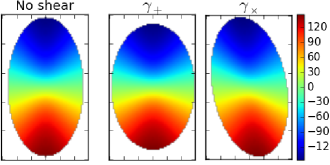
Figure 2: Velocity fields before lensing (left), after applying $\gamma_{+}=0.1$ (middle), and after applying $\gamma_{\times}=0.1$ (right). The galaxy has maximum rotation speed of 220 km/s and is inclined at 1 radian to the line of sight. The colorbar shows units of km/s.

With this in mind, the left panel of Figure 2 shows an unlensed model velocity field for $i=60^{\circ}$ and fortuitously aligned with the coordinate axes. The middle and right panels show the same field after lensing by $\gamma_{+}$ and $\gamma_{\times}$ respectively. (All fields in this figure are cropped at a consistent physical radius; this guides the eye but may overstate the power of the method, because such cuts and comparisons will not be available to the data analyst.) The right panel displays the asymmetry discussed in the introduction, which we will associate with $\gamma_{\times}$ throughout the paper. Our formalism defines the shear components with respect to sky coordinate axes rather than the galaxy axes, so in practice the asymmetry-causing component need not be $\gamma_{\times}$ as defined on the sky. Although the physical distinction is between shear components aligned and not aligned with the apparent unlensed galaxy axes, we choose not to define the components this way because in practice the unlensed axes are unknown. By defining shear components on the sky, we adopt the basis in which shear will actually be used. That said, to highlight physical behaviors we will typically align the galaxy as in Figure 2 and refer to $\gamma_{\times}$ as causing the asymmetry.

Velocity                                                                  Intensity
$i=20^{\circ}$

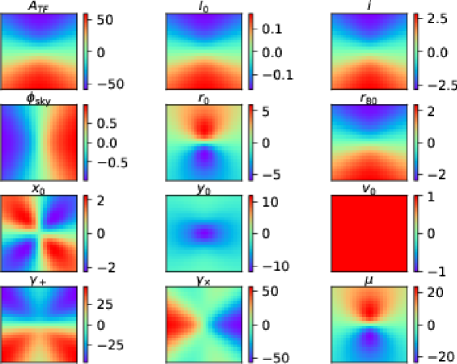
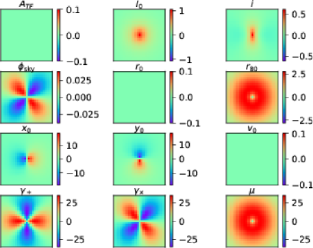
$i=60^{\circ}$

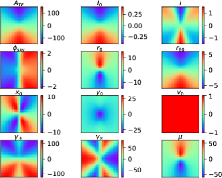
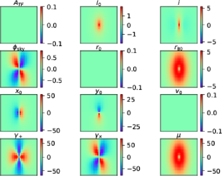
Figure 3: Partial derivatives of the velocity (left) and intensity (right) fields with respect to each of the parameters, for an inclination of 20^∘ (top row) and 60^∘ (bottom row). The colorbar units are km/s on the left, and arbitrary intensity units on the right. To keep the scales roughly the same across panels, we show the change in velocity per 0.01 change in shear and convergence. The form of the velocity field itself can be seen in the $A_{TF}$ panels on the left because that field is linear in $A_{TF}$. Similarly, the form of the intensity field can be seen in the $I_{0}$ panels on the right.

A key assumption is that the unlensed velocity field has the symmetry shown. Under this assumption, the data analyst can determine $\gamma_{\times}$ because the relevant unlensed condition is known. The effect of $\gamma_{+}$ is to change the apparent axis ratio, so measuring $\gamma_{+}$ requires knowledge of the unlensed axis ratio. That axis ratio is set by the inclination, an effect distinct from that of $\gamma_{+}$ in that inclination also changes the line-of-sight velocity. It is conceptually useful to consider the extreme case of a uniform observed velocity field, from which we can deduce that the galaxy must be viewed face-on. This implies a unlensed axis ratio of unity, so we can deduce $\gamma_{+}$ from the observed axis ratio, with no shape noise. The key is the ability to deduce a unlensed axis ratio from the velocity field amplitude; this is a way of restating the idea of Huff et al. (2013).

To go beyond this conceptual understanding we must choose quantitative models for the intensity and velocity fields. First, we define the parameter $r_{80}$, which is the radius that encircles 80% of the galaxy light. For an exponential disk, this is 2.99 times the exponential scale length. The intensity field is specified by $I=I_{0}\exp(-\frac{2.99R}{r_{80}})$, where the parameter $I_{0}$ represents the central intensity. We set the intensity uncertainty in each pixel to unity, so $I_{0}$ represents the S/N of the intensity measurement in the central pixel. The intensity uncertainty field is uniform because sky noise, rather than photon noise from the galaxy itself, is the dominant uncertainty in broadband imaging of most galaxies. We set the fiducial value of $I_{0}$ to 90, which is a high S/N reflecting the fact that bright galaxies are the likeliest targets for integral field spectroscopy. The velocity uncertainty is set by $\sigma_{v,0}$, the uncertainty in the central pixel (with a fiducial value of 10 km/s) and grows exponentially with $R$ because source photon noise is likely to be the limiting factor.

We adopt a simple arctan rotation curve: $v=v_{\rm max}\frac{2}{\pi}\arctan\frac{R}{r_{0}}$, where the factor $\frac{2}{\pi}$ ensures that $v\to v_{\rm max}$ as $r\to\infty$ given an arctan function that returns radians. We also investigated the more complicated Universal Rotation Curve (URC; Persic et al., 1996; Salucci et al., 2007) and found the results to be nearly identical; a few minor differences will be discussed in §3.8. With either form, the rotation curve has a scale length independent of the scale length describing the intensity field. If these two scales were the same, the model would be more constrained and yield higher precision, but the scales do appear to differ in observed galaxies.

$v_{\rm max}$ is related to the intensity field via the Tully-Fisher relation (TFR) as follows. The TFR empirically states that $L\propto v_{\rm max}^{n}$ where $n\approx 4$, with a scatter in luminosity or stellar mass of about 16% (Miller et al., 2011). This implies that at fixed $L$ the scatter in $v_{\rm max}$ is about 4%. For an exponential disk, the total luminosity is $L\propto I_{0}r_{80}^{2}$, so the TFR predicts $v_{\rm max}\propto(I_{0}r_{80}^{2})^{0.25}$. With our fiducial values of $I_{0}$ and $r_{80}$ (12.5 pixels), we need $v_{\rm max}=20(I_{0}r_{80}^{2})^{0.25}$ to produce a typical rotation speed around 200 km/s. Hence we define a Tully-Fisher amplitude, $A_{TF}$, with a fiducial value of unity, such that $v_{\rm max}=20A_{TF}(I_{0}r_{80}^{2})^{0.25}$. We then place a prior of $\pm 4\%$ on $A_{TF}$.

Table 1 summarizes the parameters for this model, including the nuisance parameters $x_{0},y_{0},v_{0}$ describing the galaxy position on the sky and systemic radial velocity. The units listed in this table are relevant to the forecast precision plots presented below; units are omitted for dimensionless quantities. The results can be quite sensitive to the inclination angle $i$, so $i$ will be varied in many plots rather than remaining fixed at a fiducial value.

Table 1: Model parameters

Symbol	Fiducial value	Unit	Description
$A_{TF}$	1	-	$v_{\rm max}$ as a fraction of the Tully-Fisher prediction
$I_{0}$	90	-	intensity S/N at center
$i$	varies	deg	inclination angle
$\phi_{\rm sky}$	0	deg	sky position angle of unlensed major axis
$r_{0}$	4	pixel	rotation curve scale length
$r_{80}$	12.5	pixel	radius of 80% encircled light
$x_{0}$	0	pixel	center of galaxy in $x$ coordinate
$y_{0}$	0	pixel	center of galaxy in $y$ coordinate
$v_{0}$	0	km/s	galaxy systemic radial velocity
$\gamma_{+}$	0	-	shear parallel to sky coordinates
$\gamma_{\times}$	0	-	shear at 45∘ to sky coordinates
$\mu$	1	-	magnification
Data parameters
$n_{\rm pix}$	25	pixel	field diameter
$\sigma_{v,0}$	10	km/s	uncertainty in $v$, central pixel

We construct velocity and intensity fields extending to a radius of $r_{80}$, thus encompassing 25$\times 25$ pixels each. We compute partial derivatives numerically to a relative precision of order $10^{-11}$ using the algorithm in Section 5.7 of Press et al. (1992), which we re-implement in Python. Figure 3 shows the partial derivatives of the velocity and intensity fields with respect to each parameter at two different inclinations. These figures will help readers understand which parameters are highly correlated. Note that $A_{TF}$, $I_{0}$, $i$, and $r_{80}$ have nearly identical effects on the velocity field. For $A_{TF}$ this is broken by its lack of effect on the intensity field, but $I_{0}$ and $r_{80}$ also have nearly identical effects on that field—with opposite sign, but the sign is not relevant for determining degeneracy and correlation. The effect of $i$ on the intensity field is not identical to that of $I_{0}$, but there is a good deal of overlap, indicating that the three parameters $I_{0}$, $i$, and $r_{80}$ will be highly correlated. Magnification ($\mu$) joins this family because its effect on both velocity and intensity fields is much like $-I_{0}$, and its effect on the intensity field is identical to changing the intensity scale length $r_{80}$. Finally, $r_{0}$ is linked with all these parameters because, as a rotation curve scale length, its effect on the velocity field is identical to that of magnification $\mu$. The strength of these correlations will vary with the specific values of inclination, shear, and so on: Figure 3, for example, shows that by $i=60^{\circ}$ perturbations in $i$ affect the velocity field differently than perturbations in $I_{0}$ and $r_{80}$.

For any given value of $i$, we concatenate the velocity and intensity fields into a Python data structure representing a generalized data field we denote $\vec{D}$. Denoting the set of parameters as $P$, the Fisher matrix elements are then

$$\mathcal{F}_{ij}=\sum_{\rm pixels}\vec{\sigma}^{-2}(\frac{\partial\vec{D}}{\partial P_{i}})(\frac{\partial\vec{D}}{\partial P_{j}})$$ (5)

where $i$ and $j$ index the parameters, and $\vec{\sigma}$ is the uncertainty field associated with the data field. We then invert the Fisher matrix to obtain the covariance matrix $C$. We also compute the correlation matrix $\rho\equiv D^{-1}CD^{-1}$ where $D\equiv\sqrt{\textrm{diag}(C)}$.

3 Results

3.1 Degeneracies

We find that $\frac{\partial\vec{D}}{\partial\gamma_{+}}$ is a linear combination of the other partial derivative fields. The coefficients depend on the parameter values themselves, but for concreteness we display the coefficients for our fiducial scenario at $i=30^{\circ}$:

$$\frac{\partial\vec{D}}{\partial\gamma_{+}}+199\frac{\partial\vec{D}}{\partial i}-180\frac{\partial\vec{D}}{\partial I_{0}}+4\frac{\partial\vec{D}}{\partial r_{0}}+12.5\frac{\partial\vec{D}}{\partial r_{80}}-6\frac{\partial\vec{D}}{\partial A_{\rm TF}}=0$$ (6)

Hence, a model can be transformed into another model with a different $\gamma_{+}$ value that predicts the same data, providing that we:

• increment $i$ to preserve the apparent axis ratio despite the change caused by $\gamma_{+}$. (In our setup, the unlensed apparent major axis is in the “$y$” direction while positive $\gamma_{+}$ acts to stretch the “$x$” direction, hence one must make the galaxy more edge-on to counteract positive $\gamma_{+}$.)

• decrement $I_{0}$ to preserve the apparent surface brightness. (In our model the galaxy is transparent, so making it more edge-on had the side effect of increasing the apparent surface brightness.)

• increment $r_{80}$ to preserve the observed angular size of the major axis of the intensity field. In concert with the change in inclination angle, this also preserves the apparent minor axis.

• increment $r_{0}$ to preserve the observed angular scale of the rotation curve’s rise. The coefficients on $r_{80}$ and $r_{0}$ here are equal to their fiducial values, confirming that $d\gamma_{+}$ equals the fractional change in each apparent size, as it should when $\kappa=0$.

• finally, we have to preserve the Tully-Fisher relation. To preserve the amplitude of the observed velocity-field pattern despite being more edge-on, our model must suppose a lower rotation speed, thus decreasing $A_{\rm TF}$. Alternately, the same effect can be achieved by adjusting $\mu$, which allows a lower-luminosity model to fit the intensity field.

The specific linear combination depends on the scenario, but always involves $A_{\rm TF},\mu,I_{0},i,r_{0},$ and $r_{80}$. It also involves $\phi_{\rm sky}$ if the $\gamma_{\times}$ is nonzero, and $\gamma_{\times}$ if $\phi_{\rm sky}$ is nonzero. We tested a parametrization in terms of reduced shear ($g_{+(\times)}\equiv\frac{\gamma_{+(\times)}}{1-\kappa}$) rather than shear. This did not change the set of interdependencies. We find similar dependencies parametrizing in terms of $\kappa$ rather than $\mu$. This degeneracy prevents the Fisher matrix from being inverted.

The TFR should be effective at breaking this degeneracy, in the sense that a fractional change in $\gamma_{+}$ requires a large fractional change in $A_{\rm TF}$, in tension with the TFR. But the fact that a tweak in $\mu$ can substitute for a tweak in $A_{\rm TF}$ leaves the Fisher matrix still noninvertible.

However, when finite steps are taken along the degeneracy direction, the data change quadratically with the step size, suggesting that data can indeed constrain the model. We have confirmed this with Markov Chain Monte Carlo (MCMC) explorations of the likelihood surface: our fiducial data constrain $\mu$ to slightly better than $\pm 0.1$ at all inclinations. Hence we support the Fisher forecast by placing a prior of $\pm 0.1$ on $\mu$. The fact that data constrain $\mu$ as well as all the other parameters is potentially important and will be further explored in a subsequent paper using higher order expansions of the likelihood surface (Heavens, 2016) and/or MCMC techniques.

The physical context is that $\mu=1$ in the absence of lensing; only the densest lines of sight have $\mu$ approaching 2 or more; and for those lines of sight the fact that $\mu$ is high will generally be known in advance. We also note that the weak lensing formalism used here breaks down at high magnification. Specifically, we assume that the matrix $A$ (hence the parameters $\gamma_{+}$, $\gamma_{\times}$, and $\mu$) is constant over the extent of the target galaxy, and this is not generally the case along strongly lensed lines of sight. In those cases, more traditional strong-lensing techniques will be preferred, although it is possible that the velocity field can complement the intensity field in constraining the strong-lensing reconstruction (Rizzo et al., 2018). For all these reasons, the $\mu$ uncertainty on a typical weak lensing line of sight would approach 0.1 in any case, so our prior is a good match to the physical situation. Table 2 lists the priors applied as part of our standard forecast.

Table 2: Priors

Parameter	Width (Gaussian $\sigma$)
$A_{TF}$	0.04
$\mu$	0.1

With this prior in place, we invert the Fisher matrix. Numerical instability in matrix inversion generally becomes important if the inverse of the condition number, the ratio between largest and smallest modulus eigenvalue, is not much larger than the inaccuracies in our knowledge of the matrix elements (Vallisneri, 2008). With the $\mu$ prior we find condition numbers ranging from $\approx 10^{6.5}$ at $i=10^{\circ}$ to $\approx 10^{11.5}$ at $i=80^{\circ}$. The inverse of the latter overlaps the $\sim 10^{-11}$ uncertainty in our numerical differentiation cited above. Hence, we cannot make numerically stable forecasts for galaxies close to edge-on. We limit our forecasts to those with condition number $<10^{8}$ ($i\leq 50^{\circ}$). Appendix A shows that forecasts with these condition numbers match very well with MCMC explorations of the likelihood surface. In the verified results below, the shear constraints consistently degrade as the inclination increases from $10^{\circ}$ to $50^{\circ}$, so there is little reason to push the forecast to higher inclination.

         

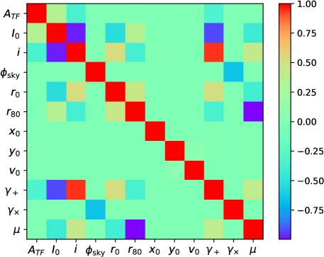
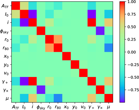
Figure 4: Correlation matrices for the $i=20^{\circ}$ (left) and $i=50^{\circ}$ (right) cases.

Figure 4 shows the resulting correlation matrices for low- and high-inclination cases. The parameters in the family discussed above ($A_{\rm TF}$, $I_{0}$, $i$, $r_{0}$, $r_{80}$, $\gamma_{+}$, and $\mu$) are indeed correlated, with some increase in correlation at higher inclination. Separately, there is an anticorrelation between $\phi_{\rm sky}$ and $\gamma_{x}$, which is moderately strong at $i=20^{\circ}$ but quite strong at $i=50^{\circ}$. This suggests that higher inclinations will yield looser constraints for both shear components. These correlations set the stage for understanding our primary products, forecasts of precision on each parameter.

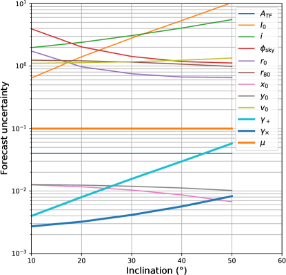
Figure 5: Forecast constraints as a function of inclination angle $i$.

3.2 Fiducial forecast

We repeat the process of building and inverting the Fisher matrix in order to present these forecasts as a function of $i$, as shown in Figure 5. The main features are:

• The $i$-dependence is dramatic: face-on targets yield much more information. This is perhaps counterintuitive because such a target will have a featureless velocity field, but in our idealized model such a featureless field carries the information that the unlensed image is exactly circular, which is most sensitive to shear.

• The $\gamma_{\times}$ precision is tighter than than the $\gamma_{+}$ precision by a factor of 1.5 (at $i{=}10^{\circ}$) to 7 (at $i{=}50^{\circ}$). This is because $\gamma_{+}$ inference depends crucially on prior knowledge of $v_{\rm max}$ and $\mu$ while $\gamma_{\times}$ inference depends on a more fundamental symmetry argument. The precision of that symmetry argument depends, of course, on the assumption that real galaxy velocity fields have negligible shearlike modes, so this assumption is one that should be tested in further work.

• In this high-S/N and well-resolved scenario, both shear components can be inferred to a precision of 0.01 or better if the target is nearly face-on. At 50^∘ (close to a typical value for randomly selected targets) $\gamma_{\times}$ can still be inferred to this precision but the constraint on $\gamma_{+}$ is less useful. (§3.4 will show that a linear combination of $\gamma_{+}$ and $\mu$ can still be constrained at this inclination.)

3.3 Dependence on Tully-Fisher prior

Tightening the Tully-Fisher (TF) prior has no effect on the $\gamma_{+}$ forecast because the dominant source of uncertainty for $\gamma_{+}$ is uncertainty in $\mu$, at least in our fiducial setup. This raises the question of how loose a TF prior is tolerable. We found a $\lesssim 10\%$ relative effect on $\gamma_{+}$ uncertainty when the prior is loosened from 0.04 to 0.08, and $\approx 30\%$ relative effect when further loosened to 0.16 (i.e., 16% scatter in rotation speed at fixed luminosity, or almost a factor of two scatter in luminosity at fixed speed). In summary, we see a substantial effect on $\gamma_{+}$ when the TF prior becomes looser than the prior on $\mu$. Conversely, the current level of TFR scatter is low enough that uncertainty in $\mu$ will remain the factor driving the $\gamma_{+}$ uncertainty for the foreseeable future.

Note that neither $\mu$ nor TF priors affect the $\gamma_{\times}$ forecast. In our idealized model, the limiting factor on $\gamma_{\times}$ precision is merely the precision and resolution of the velocity field measurements. This is unlikely to be the case in nature, where velocity fields are not perfectly orderly. An important task beyond the scope of this paper is to quantify the leading sources of $\gamma_{\times}$ uncertainty and systematic error due to natural variations from this idealized model.

3.4 Eigenvector decomposition

A striking feature of our results so far is the dramatic growth of $\gamma_{+}$ uncertainty with inclination, from about 1.5 times the $\gamma_{\times}$ uncertainty at $i=10^{\circ}$ to about 7 times the $\gamma_{\times}$ uncertainty at $i=50^{\circ}$. In this subsection we show that this is largely due to greater mixing of $\gamma_{+}$ and $\mu$ as $i$ increases. To better illustrate what happens at high inclination, we go slightly beyond our standard range of $10^{\circ}-50^{\circ}$ and use a very loose $\mu$ prior of $\pm 1$.

Figure 6 illustrates the constraints in the $(\gamma_{+},\mu)$ plane at three representative inclinations. At low inclination the constraints on $\gamma_{+}$ and $\mu$ are nearly orthogonal. This makes sense because $\mu$ should be irrelevant in the face-on case: given a uniform velocity field, the unlensed galaxy is circular so both components of shear can be determined precisely. At higher inclination, however, the constraint ellipse rotates in the $(\gamma_{+},\mu)$ plane. With the $\mu$ uncertainty remaining $\pm 1$, this rotation greatly expands the uncertainty on $\gamma_{+}$.

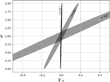
Figure 6: Constraints on $\gamma_{+}$ and $\mu$ as a function of inclination angle.

Some of the precision could be recaptured by parametrizing the lensing in terms of eigenvectors of the $(\gamma_{+},\mu)$ submatrix of the covariance matrix. These are represented graphically by the major and minor axes of the ellipses in Figure 6. Although the minor axis does increase with $i$, it increases only about one-fifth as much as the $\gamma_{+}$ uncertainty; the increase in the latter is mostly due to the eigenvector rotation.

The eigenvector decomposition could potentially be used to improve precision even at low inclination. Even the $\gamma_{+}$ width of the $i=10^{\circ}$ ellipse in Figure 6 is due largely to its $\mu$ dependence. The eigenvector decomposition defines a $\gamma_{+}$-like component with an uncertainty around 0.004, nearly as good as for $\gamma_{\times}$.

The practical impact of this reparametrization may depend on the application. It may not be useful in a cosmic shear survey. When fitting mass profiles to lenses, however, each profile predicts both $\gamma_{+}$ and $\mu$ along a given line of sight. In other words, it will predict a point in the $(\gamma_{+},\mu)$ plane depicted in Figure 6. Hence, the $i=60^{\circ}$ ellipse may have substantial power to discriminate between models despite the fact that it is compatible with a range of $\gamma_{+}$ as well as a range of $\mu$.

Even so, it is evident that high inclinations are much less constraining than low inclinations. Taking the inverse of the area of this ellipse as a figure of merit, we find that the merit degrades by a factor of six from $i=10^{\circ}$ to $i=40^{\circ}$, and by another factor of four from there to $i=60^{\circ}$.

We find similar behavior when parametrizing the lensing matrix in terms of $\kappa$ rather than $\mu$.

3.5 Dependence on target position angle

In our fiducial setup the unlensed major axis position angle is aligned with the sky coordinates ($\phi_{\rm sky}=0$), so there is no distinction between a coordinate system fixed to the sky and one fixed to the source galaxy. In principle, a coordinate system fixed to the galaxy cleanly separates the shear components into a precisely constrained one (related to the broken symmetry of the velocity field) and a less well constrained one (correlated with $\mu$). In practice, sky-based shear components must ultimately be used to interpret the shear—to relate it to a lens, for example. Hence we have defined $\gamma_{+}$ and $\gamma_{\times}$ based on sky coordinates. Our forecast uncertainties have included marginalizing over the parameter $\phi_{\rm sky}$, but our fiducial setup is still close enough to the “pure” galaxy basis that $\gamma_{+}$ and $\gamma_{\times}$ are clearly distinct. In this subsection we show that for general values of $\phi_{\rm sky}$, $\gamma_{\times}$ is no longer an eigenvector of the $(\gamma_{+},\gamma_{\times},\mu)$ space.

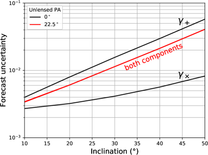
Figure 7: The effect of $\phi_{\rm sky}$ on the uncertainty of shear components defined on the sky. Unless $\phi_{\rm sky}$ is near a multiple of $45^{\circ}$ or the target is nearly face-on, neither component of shear can be measured precisely.

Figure 7 shows, along with the fiducial results, a Fisher matrix forecast for $\phi_{\rm sky}=22.5^{\circ}$, where one might expect equal precision for $\gamma_{+}$ and $\gamma_{\times}$. Indeed, the two red curves representing $\gamma_{+}$ and $\gamma_{\times}$ are identical and a factor of $\sqrt{2}$ below the fiducial $\gamma_{+}$ forecast, indicating that the uncertainty is maximally mixed between the two components. If desired, an eigenvector decomposition could be used to define two linear combinations of $\gamma_{+}$, $\gamma_{\times}$, and $\mu$ that are well measured and one that is constrained only by the prior on $\mu$. This is just one snapshot of the $\phi_{\rm sky}$-dependent mixing: at $\phi_{\rm sky}=45^{\circ}$ (not shown) $\gamma_{+}$becomes a well-constrained eigenvector, and there are intermediate degrees of mixing for intermediate values of $\phi_{\rm sky}$.

A reasonable approach to forecasting precision for randomly oriented sources would be to use the “both components” forecast in Figure 7. If, for example, we are concerned with the tangential shear of sources scattered around an axisymmetric lens, the per-source precision will vary between the $\gamma_{+}$ and $\gamma_{\times}$ curves in Figure 7, with a mean given by the “both components” curves. In this case, targets do need to be close to face-on to reach 0.01 precision; this could be limiting, as only 13% of randomly oriented disks will be within 30^∘ of face-on. In other applications it may be possible to extract more information using the eigenvector decomposition.

We remind readers that the low uncertainty for two eigenvectors stems from the idealized assumption that disk galaxies intrinsically have no shearlike modes (their intrinsic major and minor axes are equal, and their velocity fields are symmetric and locked to their intensity fields). To the extent that real galaxies depart from these assumptions, the noise floor for the eigenvectors will be higher, rendering the eigenvector decomposition (and the velocity-field method overall) less advantageous.

3.6 Dependence on shear

Because the observed velocity field is not a linear function of shear, we expect the forecast precision to depend on the shear itself. Figure 8 presents the shear constraint forecast for increasing levels of $\gamma_{\times}$, with $\gamma_{+}$ held fixed at zero. As the true $\gamma_{\times}$ increases, the $\gamma_{\times}$ precision degrades while the $\gamma_{+}$ precision is nearly unaffected. The degradation occurs particularly at low inclination where the $\gamma_{\times}$ precision had been excellent, so the $\gamma_{\times}$ forecast becomes more nearly independent of inclination. In fact, as the true $\gamma_{\times}$ becomes substantial the $\gamma_{\times}$ parameter becomes correlated with $\mu$ and its family of correlated parameters. As a result, the forecast $\gamma_{\times}$ uncertainty scales with the $\mu$ prior as well as the true $\gamma_{\times}$. For low true $\gamma_{\times}$, though, the $\gamma_{\times}$ uncertainty hits an inclination-dependent floor. This is consistent with the de Burgh-Day et al. (2015) result that $\gamma_{\times}\approx 0.01\pm 0.01$ for two nearby galaxies with presumably negligible shear, while suggesting that such precision is unobtainable along lines of sight with $\gamma_{\times}\gtrsim 0.1$.

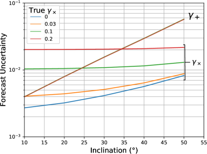
Figure 8: The uncertainty on $\gamma_{\times}$ increases when the true $\gamma_{\times}$ is substantial, due to increasing correlation with $\mu$ and related parameters. In the presence of substantial $\gamma_{\times}$ the $\gamma_{\times}$ uncertainty scales with both $\gamma_{\times}$ and the size of the $\mu$ prior, which is $\pm 0.1$ here. The $\gamma_{+}$ uncertainty is, in contrast, nearly unaffected by the true level of $\gamma_{\times}$. The true $\gamma_{+}$ is fixed at zero in this figure.

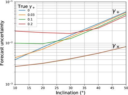
Figure 9: The $\gamma_{+}$ uncertainty depends on the true $\gamma_{+}$, but much less dramatically than the $\gamma_{\times}$ uncertainty depends on the true $\gamma_{\times}$ (Figure 8). The $\gamma_{\times}$ uncertainty is nearly unaffected by by the true level of $\gamma_{+}$. The true $\gamma_{\times}$ is fixed at zero in this figure.

Figure 9 shows the effect of varying the true $\gamma_{+}$: the $\gamma_{+}$ precision can change in either direction by factors of a few to several depending on the inclination, but there is no dramatic overall trend. There is no effect on the $\gamma_{\times}$ precision.

We also tested scenarios with mixed shear. The precision of each component appears to depend only on the true amount of that component, regardless of the true amount of the other component.

These patterns can also be understood in terms of the eigenvector decomposition. The presence of shear alters the mixing between $\gamma_{+}$, $\gamma_{\times}$, and $\mu$, and $\mu$ contamination is particularly noticeable in cases where the precision had been excellent (for $\gamma_{\times}$ generally, and for $\gamma_{+}$ at low $i$). The presence of $\gamma_{+}$ actually reduces the correlation with $\mu$ at higher inclinations and thus improves $\gamma_{+}$ inference there, but a factor of $\approx 2$ reduction from a fairly high baseline looks less dramatic on a logarithmic plot.

The eigenvector decomposition may enable useful lensing constraints in high-shear regions. Not evident in Figures 8 and 9 is the fact that the eigenvalues are nearly identical regardless of shear. An eigenvector composed mostly of $\gamma_{\times}$ but with an admixture of $\gamma_{+}$ and $\mu$ can still be constrained to high precision even at $\gamma_{\times}=0.1$. For fitting mass models, this could still be highly constraining as explained in §3.4.

3.7 Crossed slits

Obtaining full velocity-field data can be expensive, so we investigate the suggestion of Huff et al. (2013) that slit spectra be taken across the apparent major and minor photometric axes. (In our fiducial case with zero shear, these are the same as the velocity-field axes.) We implement this by masking out most pixels in the velocity-field partial derivative fields. In Figure 10 we plot the crossed-slit forecast as dashed curves, along with the standard full-field forecast as solid curves. The crossed slits increase the uncertainty by a factor of 2–3, depending only slightly on inclination.

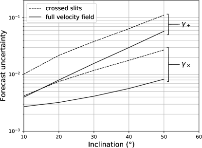
Figure 10: Shear constraints with full velocity-field observations (solid) versus crossed slits along the major and minor axes (dashed).

Although crossed slits appear to perform well for nearly face-on targets, further work is required to assess their robustness. For example, consider a galaxy whose velocity field departs from our idealized model in a few places due to substructures, one of which falls in a slit. To compare the robustness of the full velocity field and the crossed slits across a variety of realistic galaxies, simulations will be required.

3.8 Rotation Curve Model

We also made forecasts with the Universal Rotation Curve (URC; Persic et al., 1996; Salucci et al., 2007) model, which links $r_{80}$ to the radius at which the rotation curve becomes flat; in this case $r_{0}$ is still an independent parameter describing the steepness of the rise, which can lead to an overshoot. We found that the URC model leads to a small improvement when nearly edge-on (ie when the rotation curve is most apparent in observations) but otherwise yields remarkably similar shear constraints. We attribute this rotation-curve insensitivity to the basic mechanisms underlying the inference of each shear component. Inference of $\gamma_{\times}$ relies on a symmetry argument that should be insensitive to the specific form of the rotation curve. Inference of $\gamma_{+}$ is limited by lack of knowledge of $\mu$, a factor which is in no way ameliorated by adopting the URC model.

3.9 Dependence on resolution and signal-to-noise

Our fiducial setup uses velocity and intensity fields with 625 independent pixels (25 square) which, along the apparent major axis, just encloses $r_{80}=12.5$ pixels. We deliberately made our forecast agnostic as to the target redshift and instrument details, but for context, a typical disk scale length is about 4 kpc (Fathi et al., 2010). This yields $r_{80}\approx 12$ kpc, so one can think of each fiducial pixel as representing about 1 kpc. Sources behind lenses are likely to have redshifts $\approx 0.4$ and up, hence their angular diameter distances set a scale of about 5–8 kpc per arcsecond (this applies to arbitrarily high redshift sources, due to the broad maximum in angular diameter distances as a function of redshift). Therefore, a 1 kpc pixel will subtend 0.1–0.2 arcsec.

Seeing. To this point we have assumed that each pixel is completely independent, but most instruments are designed with pixel sizes smaller than the point-spread function (PSF). Therefore we tested the effect of blurring the intensity and velocity fields with a Gaussian of $\sigma=2$ pixels. This degrades the Fisher matrix forecast by only about 10% in relative terms. Hence, useful observations of the lowest-redshift targets may be possible from the ground with excellent seeing or with low-order adaptive optics, while high-redshift targets are better pursued from space or from the ground with good adaptive optics systems.

Resolution. We tested the effect of halving or doubling the angular resolution, with the field size still just enclosing $r_{80}$. For simplicity, we will describe results only for the favorable inclination $i=10^{\circ}$. Doubling (halving) the resolution halved (doubled) the forecast uncertainty on each shear component. Uncertainty decreases as pixels are added, roughly following the trend $n_{\rm pix}^{-1}$ where $n_{\rm pix}$ is the number of pixels encompassing $\pm r_{80}$ across the source major axis (and equaling the square root of the total number of pixels).

Velocity precision. Figure 11 shows the effect of varying $\sigma_{v,0}$, the uncertainty in the velocity measurement of the central pixel, at $i=10^{\circ}$. Both curves can be well fit by a simple model in which a term depending linearly on $\sigma_{v,0}$ is added in quadrature to a constant noise floor; however, the constants depend on the component and the parametrization. The $\gamma_{\times}$ component is relatively insensitive to $\sigma_{v,0}$, while the $\gamma_{+}$ component degrades more quickly. Nevertheless, Figure 11 shows that good constraints can still be obtained, at least at favorable inclinations, with lower-precision velocity data than assumed in our fiducial model. A reasonable target is 10–20 km/s: efforts to go below that meet with diminishing returns. Sacrificing additional velocity precision (i.e., exposure time) to allow targeting of more galaxies may also be a reasonable strategy.

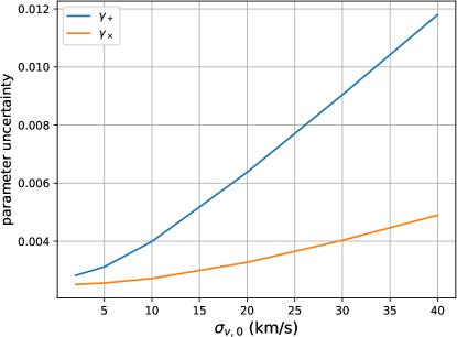
Figure 11: Shear constraints as a function of the velocity measurement uncertainty in the central pixel, at $i=10^{\circ}$.

Intensity S/N. We reduced $I_{0}$, the S/N of the central intensity pixel, from its fiducial value of 90. We found that the precision scales nearly inversely with this S/N.

Summary. The forecast precision at $i=10^{\circ}$ scales roughly as $\frac{90}{I_{0}}\frac{25}{n_{\rm pix}}$ where $I_{0}$ is the S/N of the central intensity pixel and $n_{\rm pix}$ is the number of pixels encompassing $\pm r_{80}$ across the source major axis. The dependence on velocity measurement uncertainty is not so simply captured, but 10–20 km/s is a reasonable goal for observations, with little motivation to push below that. As a caveat, we have not investigated the extent, if any, to which constraints on $\mu$ degrade with data sets less precise than our fiducial one, hence we have not quantified the effect this may in turn have on shear constraints. Simulations will be required to address this issue.

4 Summary and Discussion

Our approach has been to assume idealized and well-measured ($\sigma_{v,0}=10$ km/s) velocity fields in order to explore the potential of velocity field lensing. Our fiducial result is that at the favorable inclination $i=10^{\circ}$ the $\gamma_{\times}$ constraint can reach $0.003\frac{90}{I_{0}}\frac{25}{n_{\rm pix}}$ where $I_{0}$ is the S/N of the central intensity pixel and $n_{\rm pix}$ is the number of pixels encompassing $\pm r_{80}$ across the source major axis. The $\gamma_{+}$ constraint is 1.5–7 times looser, depending on inclination. Both constraints degrade substantially at higher inclinations.

In more detail, we find:

• The model is degenerate under infinitesimal displacements in specific directions in parameter space. However, the data change quadratically with step size along these directions, so the data can constrain all parameters. The quadratic effect can be emulated in the Fisher matrix formalism by putting a $\pm 0.1$ prior on $\mu$.

• For our fiducial zero-shear scenario, constraints on $\gamma_{\times}$ are precise to better than 0.01 for targets inclined by less than $\approx 55^{\circ}$—nearly half of all randomly inclined disks. This precision is a useful benchmark because it is roughly 20 times better than the per-galaxy precision for standard weak lensing, and also matches that found by de Burgh-Day et al. (2015). This precision, if true for both shear components, would make one velocity-field target worth roughly $20^{2}=400$ galaxy images, thus providing strong motivation to obtain the more expensive velocity-field observation.

• This precision is more difficult to reach for $\gamma_{+}$, the shear component parallel/perpendicular to the unlensed apparent major axis. With our default prior on $\mu$ ($\pm 0.1$) only targets with $i<25^{\circ}$ reach 0.01 precision on $\gamma_{+}$. This is a small minority of randomly inclined disks. Furthermore, for this select group of targets the assumption of face-on circularity is likely to be crucial, and bears further investigation.

• For either component, constraints degrade with increasing $i$. For $\gamma_{+}$ the trend is somewhat steeper so targets with substantial inclination become uninteresting. The precision can be improved somewhat if a tighter prior on $\mu$ can be justified.

• the Tully-Fisher relation is not a limiting factor. A fractional velocity scatter smaller than the prior on $\mu$ is sufficient.

• The notion of a well-measured $\gamma_{\times}$ and a less well-measured $\gamma_{+}$ is useful for conceptual understanding, but for general source PA the result is more complicated. Of the three parameters $(\gamma_{+},\gamma_{\times},\mu)$ two eigenvectors can be well measured and the third is constrained only by the prior on $\mu$. In the fiducial case, $\gamma_{\times}$ is an eigenvector but the $\gamma_{+}$-like eigenvector includes a $\mu$ component, hence constraints on $\gamma_{+}$ look worse. As $i$ increases that eigenvector rotates to include more $\mu$, so the pure $\gamma_{+}$ constraints degrade more rapidly than the $\gamma_{\times}$ constraints. If one chooses to measure the $\gamma_{+}$-like eigenvector rather than $\gamma_{+}$, the constraints degrade somewhat less rapidly with $i$.

• In the presence of shear, the nominal $\gamma_{+}$ and $\gamma_{\times}$ constraints degrade, but this is due to eigenvector rotation in the $(\gamma_{+},\gamma_{\times},\mu)$ space. The eigenvalues are equally well constrained in the presence or absence of shear.

• A per-pixel velocity uncertainty of 10–20 km/s is adequate, with smaller uncertainties yielding only marginal improvements.

• Observing a subset of the velocity field via crossed slits may be a viable strategy for reducing observing expense. In the fiducial case ($\phi_{\rm sky}=0$) this causes a factor of 2–3 degradation in the precision of each component. A more realistic assessment of crossed slits versus full velocity fields will require exploration of how real disk galaxies depart from our idealized assumptions as well as slit placement uncertainty.

Our model is highly idealized. It assumes:

• The galaxy is circular when viewed face-on.

• The velocity field is well ordered and completely described by a simple analytical function. The choice of rotation curve does not appear to matter, but the azimuthal symmetry surely matters.

• The velocity and intensity fields share a single inclination angle and PA. With the arctan rotation curve, there is no other link between the two fields (apart from the Tully-Fisher relation). With the URC, there is a link via $r_{80}$ but this does not lead to tigher constraints because the limiting factors lie elsewhere.

• The disk is infinitesimally thin. The finite thickness of real disks will likely loosen the constraints at higher inclinations, because our forecast does not account for the increased velocity width in each pixel nor for extinction.

• No additional structure such as bulges, bars, or warps. Bulges may add noise, but bars and warps seem more concerning in terms of biases. Nevertheless, de Burgh-Day et al. (2015) did succeed in inferring a plausible $\gamma_{\times}$ ($\approx 0.01\pm 0.01$) for radio observations of an unlensed nearby galaxy with a prominent gas warp, so it is possible that warps do not disturb the velocity-field symmetry in the same way that shear does. On the other hand, if the precision cited by de Burgh-Day et al. (2015) is due to typical galaxy features, future forecasts will need to account for this, with ${\sim}0.01$ becoming the $\gamma_{\times}$ noise floor. More work is needed to address this question.

The salience of warps may hinge on the velocity-field tracer: gas or stars. Gas is a convenient tracer for both radio and optical spectroscopy, but is also susceptible to inflows and outflows as well as warps. If this leads to the velocity equivalent of shape noise, the velocity-field method could become much less attractive. Stellar velocity fields are more orderly, but obtaining velocity fields from stellar absorption lines will require much more observational effort.

These observational choices are also tied to the question of whether the velocity and intensity fields must come from the same tracer. In our model the two fields are linked by a common center, inclination, and PA. The fact that our forecast is sensitive to the intensity field S/N suggests that reaching the 0.01 level does require constraints on the disk center, inclination, and PA beyond those derivable from the velocity field itself. Therefore, misalignments between intensity and velocity fields are a potential source of concern.

Recent observations indicate the potential for such misalignments. Figure 9 of Contini et al. (2016) compares the difference between the kinematic PA, as extracted from observations with the MUSE integral field spectrograph at the VLT, with the morphological PA as extracted from HST/F814W broadband images. They find one galaxy (of 27) with a large PA difference that cannot be related to poor resolution or by being nearly face-on (where PA is less well defined): the source of this difference is a bar. Even among the nearly face-on cases, they attribute some of the PA differences to structures such as spiral arms, bars, or clumps. Similarly, Wisnioski et al. (2015) find some significant offsets between the PA of broadband light and of the velocity field as traced by H$\alpha$ emission with the KMOS integral field spectrograph at the VLT. It is possible that such offsets would be reduced (albeit at additional observational expense) if stars were used to trace both velocity and intensity fields. Other potential steps to mitigate this source of error could be to model bars and spiral arms out of the intensity field, and/or to introduce a nuisance parameter representing the intensity-velocity PA offset and marginalize over it.

This concludes a long list of sources of uncertainty, yet to be quantified, that could prevent this method from being of practical use. Yet there are substantial strengths to this method as well:

• At favorable inclinations, tight constraints are achievable even with uninformative priors on $\mu$.

• The method may work well with fitting mass models to lenses. Each background source will yield a constraint that may span a range of $\gamma_{+}$, $\gamma_{\times}$, and $\mu$ but is a long, narrow ellipsoid in $(\gamma_{+},\gamma_{\times},\mu)$ space. Because a mass model predicts, for a given line of sight, a unique point in that space, the ellipsoid is likely to be highly constraining regardless of how it is oriented in that space. That said, the most highly constrained principal axis of this ellipsoid corresponds to our fiducial $\gamma_{\times}$ forecast, so this argument does not allow parameter inference better than our fiducial forecast. Rather, inferences that cannot take advantage of the eigenvectors may be limited to the precisions presented in Figures 8 and 9.

• This is a method of obtaining a high-precision shear measurement along a single line of sight, whereas traditional weak lensing enables this precision only after averaging over a large area of sky. These are different and potentially complementary types of information. The velocity field method, for example, may yield more information about localized substructures, which are effective probes of certain aspects of dark matter (see, e.g., Drlica-Wagner et al., 2019 for an overview).

Morales (2006) also argued that this method avoids some of the major systematic errors of traditional weak lensing. For example, he argues that the PSF is no longer a first-order contributor to systematics. However, our assumption that the source is well-resolved implies that the PSF would be largely irrelevant for these sources regardless of the method. He also argues that this method is less susceptible to contamination by intrinsic alignments. It is indeed robust against scenarios in which source galaxies are aligned in the absence of lensing, because the shear is measured independently on each target. But there are more subtle intrinsic alignment scenarios (Hirata & Seljak, 2004). Imagine that Galaxy A sits in a gravitational tidal field that directly affects its velocity field by perturbing the orbits of its stars, while Galaxy B is a background source lensed by that gravitational tidal field. To the extent that the velocity field perturbation in Galaxy A mimics lensing modes, it will have an “intrinsic shear” that is correlated with the lensing shear on Galaxy B. In fact, this is perhaps the most important open question here: can an external tidal field, perhaps due to a neighbor or satellite, induce shearlike perturbations in a disk’s velocity field? If so, marginalizing over a range of such velocity field models could introduce significant uncertainty. Whatever their origin, natural sources of uncertainty will degrade $\gamma_{\times}$ more than $\gamma_{+}$ because the $\gamma_{\times}$ forecast currently is limited only by the precision of the velocity measurements.

A possible extension to this method is to analyze the velocity dispersion field as well (which requires no additional observations). The dispersion field is nonuniform because the disk’s radial, tangential, and vertical dispersions contribute differently to the line-of-sight dispersion, depending on azimuth. This yields unlensed symmetry that differs from that of the velocity field: it is symmetric about both major and minor axes. However, it is unlikely that this would contribute substantially to the Fisher information, because the azimuthal variations are small.

Appendix A Verifying the Fisher forecast with an exploration of the likelihood surface

We employ the Markov Chain Monte Carlo (MCMC) code emcee (Foreman-Mackey et al., 2013) to sample the likelihood surface. emcee implements an affine-invariant sampling algorithm, and hence performs well even on highly degenerate systems, provided they are not strongly multimodal (Goodman & Weare, 2010).

For each case we generate mock data and add the fiducial amount of noise to the velocity and intensity fields. In addition to the Tully-Fisher prior used in the main text ($\pm 0.04$ on $A_{\rm{TF}}$) we place flat step function priors on other parameters to keep the model physically well defined: $A_{\rm{TF}},I_{0},r_{0},r_{80}\geq 0$; $i$ in $[0,90^{\circ})$; $\phi_{\rm sky}$ in $[0,45^{\circ})$; and $\mu>0$. Note that we do not apply the $\pm 0.1$ prior on $\mu$ used for the Fisher forecasts; the data already constrain $\mu$ to this level due to their quadratic dependence on steps in the degeneracy direction. We initialize one thousand walkers in a small ball around the correct values. We run the Markov chain for $\approx 1000$ autocorrelation times as a burn in, followed by an additional $\approx 1000$ autocorrelation times to record the positions of the walkers.

We first examine our fiducial case at the extremes of $i=10^{\circ}$ (Figure 12 and $i=50^{\circ}$ (Figure 13. In each figure, the colorscale represents the density of MCMC samples, the cyan contour represents the MCMC 68% confidence region, and the black ellipse represents the Fisher forecast for the 68% confidence region. The three least interesting parameters ($x_{0}$, $y_{0}$, and $v_{0}$) are omitted for clarity. A good match is evident throughout all panels at $i=10^{\circ}$. At $i=50^{\circ}$ there is a hint that the forecast is becoming more pessimistic than the MCMC samples. This effect is more noticeable at higher inclinations. We attribute this to increasing numerical errors as one goes to higher inclinations: the condition number at $i=50^{\circ}$ ($60^{\circ}$) is $7\times 10^{7}$ ($3\times 10^{8}$). Hence, for the fiducial setup we provide forecasts only for $i\leq 50^{\circ}$, and more generally we provide forecasts only where the condition number is ${<}10^{8}$.

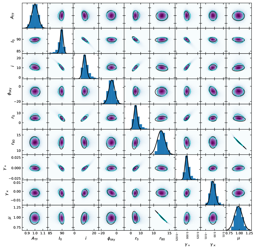
Figure 12: Corner plot for the fiducial case at $i=10^{\circ}$, showing agreement between MCMC confidence intervals and the Fisher forecast. The colorscale represents the density of MCMC samples, the cyan contour represents the MCMC 68% confidence region, and the black ellipse represents the Fisher forecast for the 68% confidence region. The forecast ellipses are centered on the densest MCMC pixel.

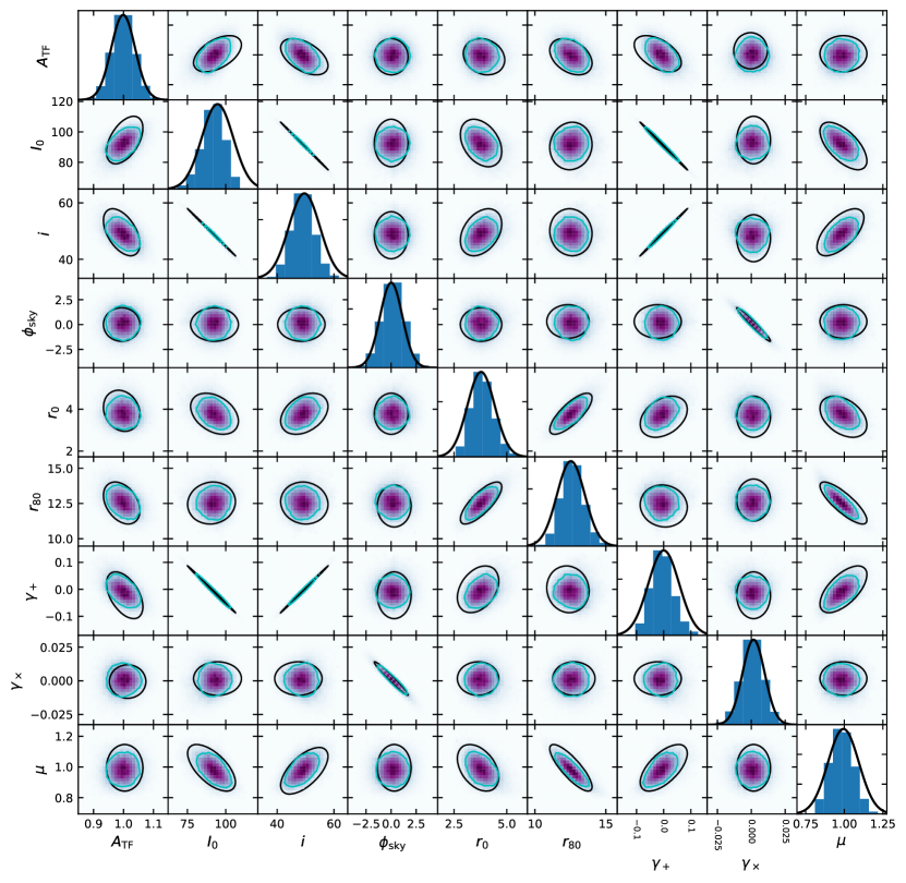
Figure 13: As for Figure 12, but at $i=50^{\circ}$.

Finally, we present a case far from our fiducial scenario: with $\phi_{\rm sky}=10^{\circ}$ and $\gamma_{+}=\gamma_{\times}=0.07$, these three parameters are highly mixed. We have also changed $r_{0}$ ($r_{80}$) to 6 (10) kpc, $I_{0}$ to 75, and $\mu$ to 1.2, with an inclination angle of $35^{\circ}$. Figure 14 shows that the forecast still accurately predicts the MCMC precision.

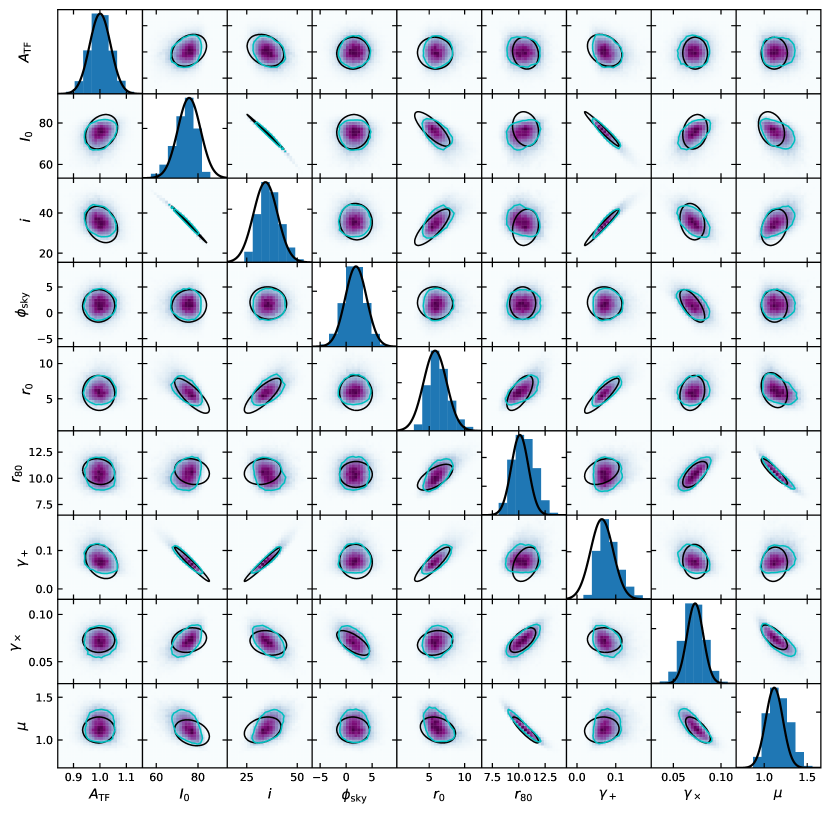
Figure 14: As for Figure 12, but for the far-from-fiducial setup described in the text. Note that the forecast contours are centered on the densest MCMC pixel, rather than the MCMC centroid.

References

- Bartelmann & Maturi (2017) Bartelmann, M., & Maturi, M. 2017, Scholarpedia, 12, 32440
- Blain (2002) Blain, A. W. 2002, ApJ, 570, L51
- Blakeslee (2001) Blakeslee, J. P. 2001, arXiv Astrophysics e-prints, astro-ph/0108253
- Contini et al. (2016) Contini, T., Epinat, B., Bouché, N., et al. 2016, A&A, 591, A49
- de Burgh-Day et al. (2015) de Burgh-Day, C. O., Taylor, E. N., Webster, R. L., & Hopkins, A. M. 2015, MNRAS, 451, 2161
- Drlica-Wagner et al. (2019) Drlica-Wagner, A., Mao, Y.-Y., Adhikari, S., et al. 2019, arXiv e-prints, arXiv:1902.01055
- Fathi et al. (2010) Fathi, K., Allen, M., Boch, T., Hatziminaoglou, E., & Peletier, R. F. 2010, MNRAS, 406, 1595
- Foreman-Mackey et al. (2013) Foreman-Mackey, D., Hogg, D. W., Lang, D., & Goodman, J. 2013, PASP, 125, 306
- Garcia-Fernandez et al. (2016) Garcia-Fernandez, M., Sánchez, E., Sevilla-Noarbe, I., et al. 2016, ArXiv e-prints, arXiv:1611.10326
- Goodman & Weare (2010) Goodman, J., & Weare, J. 2010, Communications in Applied Mathematics and Computational Science, 5, 65
- Heavens (2016) Heavens, A. 2016, Entropy, 18, 236
- Hirata & Seljak (2004) Hirata, C. M., & Seljak, U. 2004, Phys. Rev. D, 70, 063526
- Huff & Graves (2014) Huff, E. M., & Graves, G. J. 2014, ApJ, 780, L16
- Huff et al. (2013) Huff, E. M., Krause, E., Eifler, T., George, M. R., & Schlegel, D. 2013, ArXiv e-prints, arXiv:1311.1489
- Miller et al. (2011) Miller, S. H., Bundy, K., Sullivan, M., Ellis, R. S., & Treu, T. 2011, ApJ, 741, 115
- Morales (2006) Morales, M. F. 2006, ApJ, 650, L21
- Morrison et al. (2012) Morrison, C. B., Scranton, R., Ménard, B., et al. 2012, MNRAS, 426, 2489
- Persic et al. (1996) Persic, M., Salucci, P., & Stel, F. 1996, MNRAS, 281, 27
- Press et al. (1992) Press, W. H., Teukolsky, S. A., Vetterling, W. T., & Flannery, B. P. 1992, Numerical recipes in C. The art of scientific computing
- Rizzo et al. (2018) Rizzo, F., Vegetti, S., Fraternali, F., & Di Teodoro, E. 2018, MNRAS, 481, 5606
- Salucci et al. (2007) Salucci, P., Lapi, A., Tonini, C., et al. 2007, MNRAS, 378, 41
- Tully & Fisher (1977) Tully, R. B., & Fisher, J. R. 1977, A&A, 54, 661
- Vallisneri (2008) Vallisneri, M. 2008, Phys. Rev. D, 77, 042001
- Wisnioski et al. (2015) Wisnioski, E., Förster Schreiber, N. M., Wuyts, S., et al. 2015, ApJ, 799, 209