This document is the unedited author’s version of a Submitted Work that was subsequently accepted for publication in The Journal of Physical Chemistry C, copyright ^©ACS after peer review. To access the final edited and published work see: https://pubs.acs.org/doi/abs/10.1021/acs.jpcc.8b12319
Driven Liouville-von Neumann Equation for Quantum Transport and Multiple-Probe Green’s Functions

Abstract

The so called Driven Liouville-von Neumann equation is a dynamical formulation to simulate a voltage bias across a molecular system and to model a time-dependent current in a grand-canonical framework. This approach introduces a damping term in the equation of motion that drives the charge to a reference, out of equilibrium density. Originally proposed by Horsfield and co-workers, further work on this scheme has led to different coexisting versions of this equation. On the other hand, the multiple-probe scheme devised by Todorov and collaborators, known as the hairy-probes method, is a formal treatment based on Green’s functions that allows to fix the electrochemical potentials in two regions of an open quantum system. In this article, the equations of motion of the hairy probes formalism are rewritten to show that, under certain conditions, they can assume the same algebraic structure as the Driven Liouville-von Neumann equation in the form proposed by Morzan et al. [J. Chem. Phys. 2017, 146, 044110]. In this way, a new formal ground is provided for the latter, identifying the origin of every term. The performance of the different methods are explored using tight-binding time-dependent simulations in three trial structures, designated as ballistic, disordered, and resonant models. In the context of first-principles Hamiltonians the Driven Liouville-von Neumann approach is of special interest, because it does not require the calculation of Green’s functions. Hence, the effects of replacing the reference density based on the Green’s function by one obtained from an applied field are investigated, to gain a deeper understanding of the limitations and the range of applicability of the Driven Liouville-von Neumann equation.

1 Introduction

The interest in molecular conductance and electronic transport across nanostructures has inspired the development of a multiplicity of theoretical treatments to compute the current under an applied bias. The proposed schemes vary in complexity and computational cost, going from the original Landauer-Büttiker method ^{1, 2} and different static models meant to describe steady state transport, ^{3, 4, 5, 6, 7} to dynamical methodologies that take into account the time evolution of the charge density. ^{8, 9, 10, 11, 7, 6} The present article is concerned with the later class of approaches, and in particular with the subset of methods based on the so-called Driven Liouville-von Neumann (DLvN) equation. In this framework, the dynamics at the electrodes is modulated by an additional driving term that augments the standard Liouville-von Neumann equation of motion. The role of these terms is to enforce part of the density matrix associated with the electrodes to remain close to a reference density matrix, thus introducing a charge imbalance between a “source” or left lead ($L$) and a “drain” or right lead ($R$). This driving term originally takes the form of a difference between the time-dependent density matrix $\hat{\rho}(t)$, and a reference density matrix $\hat{\rho}_{0}$,

$$\dot{\hat{\rho}}(t)=-\frac{i}{\hbar}[\hat{H},\hat{\rho}(t)]-\Gamma(\hat{\rho}(t)-\hat{\rho}^{0})$$ (1)

where $\hat{H}$ is the electron Hamiltonian, $\Gamma$ is the driving rate parameter, and the matrix $\hat{\rho}^{0}$ can be defined as follows:

$${\rho}_{ij}^{0}=\left\{\begin{array}[]{ll}\rho_{ij}(t_{0})&\text{if $i,j$ $\in$ $L\cup R$ }\\ \rho_{ij}(t)&\text{if $i,j$ $\notin$ $L\cup R$ }\\ \end{array}\right.$$ (2)

This type of approach was first introduced by Horsfield and co-workers ^{12, 13} as an intuitive way of including at the level of the density matrix the circulation of charge between the electrodes, and it was further enriched by the work of Nitzan ¹⁴ and Mazziotti ¹⁵. These ideas were later taken on by Hod and co-workers ^{16, 17, 18, 19} and reelaborated by deriving the driving terms from the theory of complex absorbing potentials. In doing so, they arrived at a modified form in which coherences were damped to zero,

$$\dot{\hat{\rho}}(t)=-\frac{i}{\hbar}[\hat{H},\hat{\rho}(t)]-\frac{\Gamma}{2}\begin{bmatrix}2(\hat{\rho}_{LL}-\hat{\rho}_{LL}^{0})&\hat{\rho}_{LC}&2\hat{\rho}_{LR}\\ \hat{\rho}_{CL}&0&\hat{\rho}_{CR}\\ 2\hat{\rho}_{RL}&\hat{\rho}_{RC}&2(\hat{\rho}_{RR}-\hat{\rho}_{RR}^{0})\\ \end{bmatrix},$$ (3)

that improved the stability of the calculations and the steady-state convergence, and that was shown to satisfy Pauli’s principle regardless of the initial conditions. ¹⁶ Franco and collaborators presented a formal derivation of this formula from the theory of non-equilibrium Green’s functions, demonstrating that it can accurately capture time-dependent transport phenomena.²⁰ More recently, Zelovich et al. proposed a strategy to replace the single rate parameter $\Gamma$ by diagonal matrices containing the broadening factors corresponding to the lead states.²¹ These factors can be computed from the self-energies of the electrodes, thus providing a parameter-free version of the Driven Liouville-von Neumann approach.²¹

Because of its conceptual simplicity and good compromise between computational cost and physical accuracy, the DLvN method has attracted significant attention, and several further refinements of its implementation and analysis of its theoretical foundation were made. Among these, of particular relevance is the adaptation to a first-principles real-time TDDFT framework carried out by Morzan and co-authors,²² where an observed imbalance between injection and absorption of charge during the dynamics prompted a reformulation of the driving term. In an orthonormal basis, this equation of motion assumes the following structure:

$$\dot{\hat{\rho}}(t)=-\frac{i}{\hbar}[\hat{H},\hat{\rho}(t)]-\frac{\Gamma}{2}\begin{bmatrix}2(\hat{\rho}_{LL}-\hat{\rho}_{LL}^{0})&\hat{\rho}_{LC}-\hat{\rho}_{LC}^{0}&2(\hat{\rho}_{LR}-\hat{\rho}_{LR}^{0})\\ \hat{\rho}_{CL}-\hat{\rho}_{CL}^{0}&0&\hat{\rho}_{CR}-\hat{\rho}_{CR}^{0}\\ 2(\hat{\rho}_{RL}-\hat{\rho}_{RL}^{0})&\hat{\rho}_{RC}-\hat{\rho}_{RC}^{0}&2(\hat{\rho}_{RR}-\hat{\rho}_{RR}^{0})\\ \end{bmatrix}$$ (4)

where the subscripts indicate the corresponding blocks of the time-dependent density matrix, and $\hat{\rho}^{0}$ denotes a reference, time-independent density matrix. A major change with respect to previous expressions is that here all off-diagonal contributions are damped to their reference values (obtained e.g. from the polarized density matrix). This proved to be important for charge conservation and an appropriate balance between incoming and outgoing currents in the relatively small models tractable in TDDFT simulations.²² Despite intuitively justifying this modification both from a numerical standpoint and interpreting it as a change in the boundary conditions, no formal theoretical derivation was provided at the time.

In parallel with these developments, a different driving term for the Liouville-von Neumann equation was put forward by Todorov and co-workers.¹⁰ This new embedding method called multiple-probe or “hairy probes” (HP), formally derived a different structure of the driving term via the application of Green’s functions and the Lippmann-Schwinger equation. ^{10, 23} In spite of its good results and wide range of applicability,^{24, 25, 26} its relationship with the reference density driving method remained undetermined.

The objective of the present study is to bridge the gap between the two methodologies: the heuristic formulation of the Driven Liouville-von Neumann equation, and the hairy-probes scheme. For that purpose, we have been able to rewrite the driving terms of the HP theory into two terms, one of which resembles the damping term of the reference density approach. In doing so we have found that the latest addition of Morzan and co-workers is the most compatible with HP, thus finally providing a formal framework for their correction of the non-diagonal blocks of the driving term. Through the application of these schemes to a series of model systems, we better characterize these methodologies for different situations and shed light on the reliability of the equation of motion including the driving term with the reference density matrix $\hat{\rho}^{0}$.

In the next two sections we introduce the theoretical and methodological framework for this work: we first show how the HP theory can be rewritten to arrive to the Driven Liouville-von Neumann equation plus an additional term (section 2), and then provide a brief description of the models employed in the simulations (section 3). In section 4 we examine the impact that the progressive simplifications of the HP equation have on the accuracy of the physical description of these systems. After that we examine the effect that some of the relevant parameters of the models have on the baseline performance of these different approximations. In particular, we will focus on the $\Gamma$ parameter (section 5) and the shape of the field used to generate the reference matrix in the DLvN scheme (section 6). Finally, in section 7, we discuss the differences between the two forms of the DLvN equation reported in the literature: the one emerging from the truncation of the HP method (eq. 4), and the one proposed by Hod and co-workers (eq. 3).

2 Recasting the multiple-probe equations of motions

We consider in this work a system formed by a central molecule or device, identified hereafter with the symbol $C$, coupled to a right and a left electrode (or lead), denoted as regions $R$ and $L$ respectively. In the multiple-probes framework this system is embedded in an implicitly represented environment via the coupling of each atom of the left and right leads to an external probe, which in isolation has a retarded and an advanced surface Green’s function $g^{\pm}_{j}(E)$ and a surface local density of states $d_{j}(E)=-\pi^{-1}\Im g^{+}_{j}(E)$.¹⁰ These probes have fixed electrochemical potentials $\mu_{L}$ and $\mu_{R}$, depending on whether they are connected to the left or right electrode, with Fermi-Dirac distributions $f_{L}(E)$ and $f_{R}(E)$. For this model, and assuming that the Hamiltonian of the system is time-independent, the HP theory provides the following equation of motion for the electronic density (see eq. 38 in reference  ¹⁰):

$$i\hbar\dot{\hat{\rho}}_{S}(t)=[\hat{H}_{S},\hat{\rho}_{S}(t)]+\hat{\Sigma}^{+}\hat{\rho}_{S}(t)-\hat{\rho}_{S}(t)\hat{\Sigma}^{-}+\int[\hat{\Sigma}^{<}(E)\hat{G}^{-}_{S}(E)-\hat{G}^{+}_{S}(E)\hat{\Sigma}^{<}(E)]dE$$ (5)

where $\hat{\rho}$ is the time-dependent density matrix, $\hat{H}$ is the electron Hamiltonian, subscript $S$ refers to the full system ($L$, $C$ and $R$ sections), and the $\hat{\Sigma}$ and $\hat{G}$ matrices are the system’s self-energy and Green’s function. We also assume that (i) all probes interact with the electrodes through the same coupling term $\gamma$, and (ii) the wideband limit applies to the probes so that their density of states becomes a constant, $d_{j}(E)=d$. In these conditions, these matrices adopt the following form:

$$\hat{\Sigma}^{\pm}=\hat{\Sigma}^{\pm}_{L}+\hat{\Sigma}^{\pm}_{R}=-\frac{i\Gamma}{2}\cdot\hat{P}_{L}-\frac{i\Gamma}{2}\cdot\hat{P}_{R}=\left(\hat{\Sigma}^{\mp}\right)^{\dagger},$$ (6)

$$\hat{\Sigma}^{<}(E)=\frac{\Gamma}{2\pi}\cdot f_{L}(E)\cdot\hat{P}_{L}+\frac{\Gamma}{2\pi}\cdot f_{R}(E)\cdot\hat{P}_{R},$$ (7)

$$\hat{G}^{\pm}_{S}(E)=\left(E\cdot\hat{P}_{S}-\hat{H}_{S}-\hat{\Sigma}^{\pm}\right)^{-1}.$$ (8)

In the above equations, $\Gamma=2\pi\gamma^{2}d$, and $f_{L}(E)$ and $f_{R}(E)$ correspond to the Fermi-Dirac distributions for the left and right probes. The matrices $\hat{P}_{L}$ and $\hat{P}_{R}$ are the corresponding projector operators, with $\hat{P}_{S}$ being the projection over the whole explicit system (i.e. the identity).

We will now take equation 5 as the starting point for our derivation. Our goal in this section is to express it in terms of a difference between weighted density matrices—one corresponding to the current state of the system and the other to a reference system—that assumes the form of the driving term in the DLvN equations.

For this, we focus on the second ($\hat{\Sigma}^{+}\hat{\rho}_{S}(t)-\hat{\rho}_{S}(t)\hat{\Sigma}^{-}$) and third ($\int[\hat{\Sigma}^{<}(E)\hat{G}^{-}_{S}(E)-\hat{G}^{+}_{S}(E)\hat{\Sigma}^{<}(E)]dE$) terms on the right hand side of equation 5, and examine separately each of the sub-blocks corresponding to the orbitals of the electrodes ($L$, $R$) and of the device ($C$). The first thing to note is that, since all $\hat{\Sigma}$ matrices contain projections on the leads only, the second and third terms will vanish in the central block:

$$i\hbar\dot{\hat{\rho}}_{CC}(t)=\left([\hat{H}_{S},\hat{\rho}_{S}(t)]\right)_{CC}.$$ (9)

In turn, the off-diagonal blocks of the second term can be expanded as:

$$\hat{\Sigma}^{+}\hat{\rho}_{S}-\hat{\rho}_{S}\hat{\Sigma}^{-}=-\frac{i\Gamma}{2}\left(\hat{P}_{L}\hat{\rho}_{S}+\hat{P}_{R}\hat{\rho}_{S}+\hat{\rho}_{S}\hat{P}_{L}+\hat{\rho}_{S}\hat{P}_{R}\right)$$

$$=-\frac{i\Gamma}{2}\left(2\hat{\rho}_{LL}+2\hat{\rho}_{LR}+2\hat{\rho}_{RL}+2\hat{\rho}_{RR}+\hat{\rho}_{LC}+\hat{\rho}_{CL}+\hat{\rho}_{RC}+\hat{\rho}_{CR}\right)$$ (10)

where for conciseness we have omitted the time-dependence of $\hat{\rho}$. In matrix form, this can be written as:

$$\hat{\Sigma}^{+}\hat{\rho}_{S}-\hat{\rho}_{S}\hat{\Sigma}^{-}=-\frac{i\Gamma}{2}\begin{bmatrix}2\hat{\rho}_{LL}&\hat{\rho}_{LC}&2\hat{\rho}_{LR}\\ \hat{\rho}_{CL}&0&\hat{\rho}_{CR}\\ 2\hat{\rho}_{RL}&\hat{\rho}_{RC}&2\hat{\rho}_{RR}\\ \end{bmatrix}.$$ (11)

We now turn our attention to the third term on the right hand side of equation 5, considering separately each off-diagonal block. For the upper left one, we have:

$$\int[\hat{\Sigma}^{<}(E)\hat{G}^{-}_{S}(E)-\hat{G}^{+}_{S}(E)\hat{\Sigma}^{<}(E)]_{LL}dE=\frac{\Gamma}{2\pi}\int\left(f_{L}(E)\hat{P}_{L}\hat{G}_{S}^{-}(E)\hat{P}_{L}-f_{L}(E)\hat{P}_{L}\hat{G}_{S}^{+}(E)\hat{P}_{L}\right)dE$$

$$=\frac{\Gamma}{2\pi}\hat{P}_{L}\cdot\int f_{L}(E)\left[\hat{G}_{S}^{-}(E)-\hat{G}_{S}^{+}(E)\right]dE\cdot\hat{P}_{L}=i\Gamma\hat{P}_{L}\cdot\int f_{L}(E)\hat{D}_{S}(E)dE\cdot\hat{P}_{L}$$ (12)

where we used the relation between the Green’s function and the density of states matrix $\hat{D}_{S}(E)=(2\pi i)^{-1}\left(\hat{G}_{S}^{-}(E)-\hat{G}_{S}^{+}(E)\right)$. The integral in the last term of equation 12 defines a fictitious equilibrium density matrix with an electronic distribution $f_{L}$ corresponding to the left probes, that we will denote $\hat{\rho}^{0L}$. After applying on the left and on the right the projection operator associated with the upper left block, we arrive at the final result,

$$\int[\hat{\Sigma}^{<}(E)\hat{G}^{-}_{S}(E)-\hat{G}^{+}_{S}(E)\hat{\Sigma}^{<}(E)]_{LL}dE=i\Gamma\cdot\hat{P}_{L}\cdot\hat{\rho}^{0L}\cdot\hat{P}_{L}=i\Gamma\cdot\hat{\rho}^{0L}_{LL}.$$ (13)

For the $RR$ sub-matrix we get an analogous expression, but with the $R$ projectors and the Fermi-Dirac distribution for the right probes, which defines a different reference density matrix $\hat{\rho}^{0R}$,

$$\int[\hat{\Sigma}^{<}(E)\hat{G}^{-}_{S}(E)-\hat{G}^{+}_{S}(E)\hat{\Sigma}^{<}(E)]_{RR}dE=i\Gamma\hat{P}_{R}\cdot\int f_{R}(E)\hat{D}_{S}(E)dE\cdot\hat{P}_{R}=i\Gamma\cdot\hat{\rho}^{0R}_{RR}.$$ (14)

To evaluate the off-diagonal terms involving the central region (blocks LC, CL, RC, and CR), we first observe that in all these cases part of the integrand vanishes when operating on $\hat{\Sigma}^{<}$ due to the contiguous application of projectors belonging to different regions,

$$\int[\hat{\Sigma}^{<}(E)\hat{G}^{-}_{S}(E)-\hat{G}^{+}_{S}(E)\hat{\Sigma}^{<}(E)]_{LC}dE=\int\left(\hat{P}_{L}\hat{\Sigma}^{<}(E)\hat{G}_{S}^{-}(E)\hat{P}_{C}-\hat{P}_{L}\hat{G}_{S}^{+}(E)\hat{\Sigma}^{<}(E)\hat{P}_{C}\right)dE$$

$$=\frac{\Gamma}{2\pi}\int f_{L}(E)\hat{P}_{L}\hat{G}_{S}^{-}(E)\hat{P}_{C}dE=\frac{\Gamma}{2\pi}\hat{P}_{L}\cdot\int f_{L}(E)\hat{G}_{S}^{-}(E)dE\cdot\hat{P}_{C}.$$ (15)

Similarly,

$$\int[\hat{\Sigma}^{<}(E)\hat{G}^{-}_{S}(E)-\hat{G}^{+}_{S}(E)\hat{\Sigma}^{<}(E)]_{CL}dE=-\frac{\Gamma}{2\pi}\hat{P}_{C}\cdot\int f_{L}(E)\hat{G}_{S}^{+}(E)dE\cdot\hat{P}_{L}.$$ (16)

To recover the density of states from just one of the Green’s matrices, we rewrite the latter in the following way:

$$\hat{G}_{S}^{-}(E)=\left(\frac{\hat{G}_{S}^{-}(E)}{2}-\frac{\hat{G}_{S}^{+}(E)}{2}\right)+\left(\frac{\hat{G}_{S}^{-}(E)}{2}+\frac{\hat{G}_{S}^{+}(E)}{2}\right)=i\pi\hat{D}_{S}(E)+\hat{G}_{S}^{\Re}(E)$$ (17)

$$-\hat{G}_{S}^{+}(E)=\left(\frac{\hat{G}_{S}^{-}(E)}{2}-\frac{\hat{G}_{S}^{+}(E)}{2}\right)+\left(-\frac{\hat{G}_{S}^{-}(E)}{2}-\frac{\hat{G}_{S}^{+}(E)}{2}\right)=i\pi\hat{D}_{S}(E)-\hat{G}_{S}^{\Re}(E),$$ (18)

for which we have defined the matrix $\hat{G}_{S}^{\Re}(E)=\frac{1}{2}(\hat{G}_{S}^{-}(E)+\hat{G}_{S}^{+}(E))$. Inserting equations 17 and 18 in equations 15 and 16, we arrive at

$$\int[\hat{\Sigma}^{<}(E)\hat{G}^{-}_{S}(E)-\hat{G}^{+}_{S}(E)\hat{\Sigma}^{<}(E)]_{LC}dE=$$

$$\frac{i\Gamma}{2}\hat{P}_{L}\cdot\int f_{L}(E)\hat{D}_{S}(E)dE\cdot\hat{P}_{C}+\frac{\Gamma}{2\pi}\hat{P}_{L}\cdot\int f_{L}(E)\hat{G}_{S}^{\Re}(E)dE\cdot\hat{P}_{C}=\frac{i\Gamma}{2}\hat{\rho}^{0L}_{LC}+\frac{\Gamma}{2\pi}\hat{\Omega}^{L}_{LC}.$$ (19)

Similarly

$$\int[\hat{\Sigma}^{<}(E)\hat{G}^{-}_{S}(E)-\hat{G}^{+}_{S}(E)\hat{\Sigma}^{<}(E)]_{CL}dE=\frac{i\Gamma}{2}\hat{\rho}^{0L}_{CL}-\frac{\Gamma}{2\pi}\hat{\Omega}^{L}_{CL}$$ (20)

where we have introduced the matrix $\hat{\Omega}^{L/R}=\int f_{L/R}(E)\hat{G}_{S}^{\Re}(E)dE$. The terms involving the right lead can be treated on the same footing, to obtain an analogous result but incorporating the reference density and $\hat{\Omega}$ corresponding to the right region,

$$\int[\hat{\Sigma}^{<}(E)\hat{G}^{-}_{S}(E)-\hat{G}^{+}_{S}(E)\hat{\Sigma}^{<}(E)]_{RC}dE=\frac{i\Gamma}{2}\hat{\rho}^{0R}_{RC}+\frac{\Gamma}{2\pi}\hat{\Omega}^{R}_{RC}$$ (21)

$$\int[\hat{\Sigma}^{<}(E)\hat{G}^{-}_{S}(E)-\hat{G}^{+}_{S}(E)\hat{\Sigma}^{<}(E)]_{CR}dE=\frac{i\Gamma}{2}\hat{\rho}^{0R}_{CR}-\frac{\Gamma}{2\pi}\hat{\Omega}^{R}_{CR}.$$ (22)

To complete the derivation, we consider the two remaining blocks that couple both leads together ($LR$, $RL$):

$$\int[\hat{\Sigma}^{<}(E)\hat{G}^{-}_{S}(E)-\hat{G}^{+}_{S}(E)\hat{\Sigma}^{<}(E)]_{LR}dE=\frac{\Gamma}{2\pi}\int\left(f_{L}(E)\hat{P}_{L}\hat{G}_{S}^{-}(E)\hat{P}_{R}-f_{R}(E)\hat{P}_{L}\hat{G}_{S}^{+}(E)\hat{P}_{R}\right)dE$$

$$=\frac{\Gamma}{2\pi}\hat{P}_{L}\cdot\int\left(f_{L}(E)\hat{G}_{S}^{-}(E)-f_{R}(E)\hat{G}_{S}^{+}(E)\right)dE\cdot\hat{P}_{R}.$$ (23)

The expression within the brackets can be rewritten introducing relations 17 and 18 to elicit the reference density and omega matrices,

$$\int\left(f_{L}(E)\hat{G}_{S}^{-}(E)-f_{R}(E)\hat{G}_{S}^{+}(E)\right)dE$$

$$=\int\left(i\pi f_{L}(E)\hat{D}_{S}(E)+f_{L}(E)\hat{G}_{S}^{\Re}(E)+i\pi f_{R}(E)\hat{D}_{S}-f_{R}(E)\hat{G}_{S}^{\Re}\right)dE$$

$$=i\pi\hat{\rho}_{S}^{0L}+\hat{\Omega}_{S}^{L}+i\pi\hat{\rho}_{S}^{0R}-\hat{\Omega}_{S}^{R},$$ (24)

leading to the following result:

$$\int[\hat{\Sigma}^{<}(E)\hat{G}^{-}_{S}(E)-\hat{G}^{+}_{S}(E)\hat{\Sigma}^{<}(E)]_{LR}dE=\frac{i\Gamma}{2}\left(\hat{\rho}_{LR}^{0L}+\hat{\rho}_{LR}^{0R}\right)+\frac{\Gamma}{2\pi}\left(\hat{\Omega}_{LR}^{L}-\hat{\Omega}_{LR}^{R}\right)$$ (25)

which combines the left and right probes populated matrices. The $RL$ block is treated analogously, to obtain:

$$\int[\hat{\Sigma}^{<}(E)\hat{G}^{-}_{S}(E)-\hat{G}^{+}_{S}(E)\hat{\Sigma}^{<}(E)]_{RL}dE=\frac{i\Gamma}{2}\left(\hat{\rho}_{RL}^{0L}+\hat{\rho}_{RL}^{0R}\right)+\frac{\Gamma}{2\pi}\left(\hat{\Omega}_{RL}^{R}-\hat{\Omega}_{RL}^{L}\right).$$ (26)

Thus, the third term in equation 5 can in matrix form be written as:

$$\int[\hat{\Sigma}^{<}(E)\hat{G}^{-}_{S}(E)-\hat{G}^{+}_{S}(E)\hat{\Sigma}^{<}(E)]dE$$

$$=\frac{i\Gamma}{2}\begin{bmatrix}2\hat{\rho}^{0L}_{LL}&\hat{\rho}^{0L}_{LC}&\hat{\rho}^{0L}_{LR}+\hat{\rho}^{0R}_{LR}\\ \hat{\rho}^{0L}_{CL}&0&\hat{\rho}^{0R}_{CR}\\ \hat{\rho}^{0L}_{RL}+\hat{\rho}^{0R}_{RL}&\hat{\rho}^{0R}_{RC}&2\hat{\rho}^{0R}_{RR}\\ \end{bmatrix}+\frac{\Gamma}{2\pi}\begin{bmatrix}0&\hat{\Omega}^{L}_{LC}&\hat{\Omega}^{L}_{LR}-\hat{\Omega}^{R}_{LR}\\ -\hat{\Omega}^{L}_{CL}&0&-\hat{\Omega}^{R}_{CR}\\ \hat{\Omega}^{R}_{RL}-\hat{\Omega}^{L}_{RL}&\hat{\Omega}^{R}_{RC}&0\\ \end{bmatrix}$$ (27)

where the first matrix on the right hand side will be referred to as the “region-weighted reference density matrix”, or simply reference density matrix.

Finally, collecting all the pieces together, the HP master equation can be rewritten in the following way:

$$\dot{\hat{\rho}}(t)=-\frac{i}{\hbar}[\hat{H}_{S},\hat{\rho}_{S}(t)]-\frac{\Gamma}{2\hbar}\begin{bmatrix}2(\hat{\rho}_{LL}-\hat{\rho}^{0L}_{LL})&\hat{\rho}_{LC}-\hat{\rho}^{0L}_{LC}&2\left(\hat{\rho}_{LR}-\frac{\hat{\rho}^{0L}_{LR}+\hat{\rho}^{0R}_{LR}}{2}\right)\\ \hat{\rho}_{CL}-\hat{\rho}_{CL}^{0L}&0&\hat{\rho}_{CR}-\hat{\rho}_{CR}^{0R}\\ 2\left(\hat{\rho}_{RL}-\frac{\hat{\rho}^{0L}_{RL}+\hat{\rho}^{0R}_{RL}}{2}\right)&\hat{\rho}_{RC}-\hat{\rho}^{0R}_{RC}&2(\hat{\rho}_{RR}-\hat{\rho}^{0R}_{RR})\\ \end{bmatrix}$$

$$-\frac{i\Gamma}{2\pi\hbar}\begin{bmatrix}0&\hat{\Omega}_{LC}^{L}&\hat{\Omega}_{LR}^{L}-\hat{\Omega}_{LR}^{R}\\ -\hat{\Omega}^{L}_{CL}&0&-\hat{\Omega}^{R}_{CR}\\ \hat{\Omega}^{R}_{RL}-\hat{\Omega}^{L}_{RL}&\hat{\Omega}^{R}_{RC}&0\\ \end{bmatrix}$$ (28)

We have thus arrived at a mathematical structure that is very similar to that of the DLvN scheme as presented in equation 4. By this we mean that the second term has the form of a block-weighted difference between the current time dependent density matrix and a reference density matrix. The implications of the definition of this reference matrix and the impact of including or excluding the remaining $\Omega$-term are analyzed in the remainder of this work.

3 Equations of motion, model systems, and time propagation

In what follows we assess and compare the performance of three different implementations of the HP equation of motion: (i) the full formula 28; (ii) a version excluding the $\Omega$-term; and (iii) same as (ii), but where the region-weighted reference density matrix is computed using a step-shaped field encoding the bias potential. In the latter, notice that $\hat{\rho}^{0L}$ and $\hat{\rho}^{0R}$ are the same matrix $\hat{\rho}^{0}$, corresponding to the polarized density in the presence of a step-field, and thus the equation of motion becomes identical to equation 4. These three schemes (i), (ii) and (iii), will be referred to as “full-HP”, “partial-HP”, and “step-potential” methods, or, for short, F-HP, P-HP, and ST-P, respectively. As mentioned above, the mathematical structure of the P-HP approach resembles closely the one of the DLvN equation 4, implemented in this study as the ST-P method. In particular, the driving term arising in the HP formula reinstates the damping of the coherences to the equilibrium values. In this sense, the ST-P scheme can also be thought of as an approximation to the P-HP method with an alternative reference density matrix. The motivation to explore it is to bypass the calculation of Green’s functions, which becomes especially appealing in the context of ab-initio Hamiltonians.

For comparison purposes, we also consider in this work the alternative form of DLvN given by equation 3, which hereafter will be referred to as DLvN-z, whereas the version in equation 4 will be denoted as DLvN-e (since these two equations damp the lead-molecule coherences to zero and to their equilibrium values, respectively). It is important to note from this is that “ST-P” and “DLvN-e” refer to the exact same method: we will in general use the first notation when comparing only with other HP-derived methods, and the second one when also including the other version of the DLvN equation.

To examine the performance of these different equations of motion, a series of model systems were chosen as case studies in numerical simulations. All these systems consist of linear chains of atoms arranged in different spatial configurations (see below). The electronic structure is represented by a tight-binding Hamiltonian with an orthonormal one-electron basis, using the model presented by Sutton and co-workers ²⁷ (other possible, more elaborate electronic models are discussed in  ²⁶). This scheme adopts a single orbital $|j\rangle$ per atom (or site), coupled with each other by nearest-neighbour hopping terms that only depend on the distance between sites. The onsite energies will in general be identical for all atoms, except in the “disordered” model (see below), or in the presence of an external field used to obtain the reference matrix.

For the HP method, the potential difference $\Delta V$ between the left and right probes determines the Fermi-Dirac distributions according to the corresponding electrochemical potentials $\mu_{L}=+\Delta V/2$ and $\mu_{R}=-\Delta V/2$. The presence of an external field (to generate the reference density to be used either in the modified HP or the DLvN schemes) is simulated through the modification of the onsite energies. The shape of this field is a matter of analysis in section 6, but for the simulations in sections 4 and 5, constant values of $+\Delta V/2$ and $-\Delta V/2$ were used for the atoms in the left and right leads (respectively), whereas the onsite energies of the atoms in the device were left unmodified.

The time integration of the equations of motion for the electrons was performed by using a simple Leapfrog algorithm, and for all the simulations presented in this work the time-step chosen was of 0.005 fs. The driving term was weighted by an extra time dependent factor that grows linearly from 0 to 1 in the first few steps of the propagation. Tests were performed to check that the time step and the slope of the initial ramp did not affect the shape of the current.

Simulations were performed on three basic systems characterized by the configuration of their central region ($C$). In all systems the electrodes $L$ and $R$ are made of 200 atoms, except for some results shown in section 7 in which shorter leads of 50 atoms were explored. In all cases the systems are metallic, exhibiting a half-filled conduction band. These three systems are:

• Ballistic: all atoms in the system ($S$) are equally spaced by 2.5 $\AA$, involving a hopping integral of -3.88 eV (which corresponds to the tight-binding reference parameters for gold²⁷). The on-site energy is the same for all atoms. There are 21 atoms in the central region $C$.

• Disordered: this system has the exact same geometry as the ballistic (same number of atoms all equally spaced), but with a different on-site energy for every atom belonging to the central region $C$. These different on-site energies were randomly generated using a homogeneous distribution with values between plus and minus the absolute value of the hopping term above.

• Resonant: all sites are equally spaced as in the previous cases, with the exception of two distances separating a group of 15 atoms in the center of the device, from two groups of 9 atoms on each end, connected to the electrodes. All of these belong to the $C$ region, as can be seen in Figure 1. These two bonds were 0.5 Å longer than the rest. The on-site energies are the same for all atoms, but the hopping terms of the longer bonds are -1.88 eV.

Figure 1: Scheme of the resonant system. All on-site energies are the same.

Modified versions of the resonant system were later used in section 6. Instead of having a 9-15-9 configuration of the central region (with the dash standing for the longer separation), these are 9-45-9 and 30-15-30.

4 The components of the driving term and their role

Figure 2 depicts the current as a function of time for transport simulations based on the F-HP, P-HP, ST-P (or DLvN-e), and DLvN-z methods. It is seen that the currents reach a stable steady state, regardless of the method, model system, and the value of $\Gamma$. The upper, middle and lower panels of Figure 2, correspond to the ballistic, the resonant, and the disordered models, respectively, for an applied bias of 1.5 V (the same stable behavior is found for other bias). Left and right panels show the currents for $\Gamma$ equal to 0.1 eV and 0.6 eV. It can be seen that for large couplings, the steady state is reached faster, and that in none of the cases is there any ambiguity in the identification of the final current, since it typically converges to a precise value within the first 10 - 40 fs of dynamics, depending on $\Gamma$. While the figures present the current for the initial 400 fs, most of the simulations have been evolved for up to 1 ps, without the detection of instabilities.

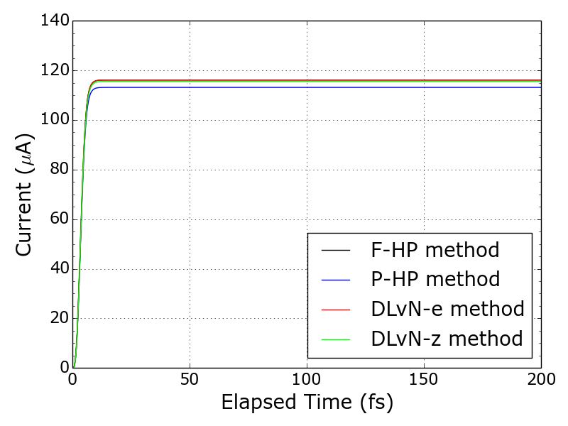
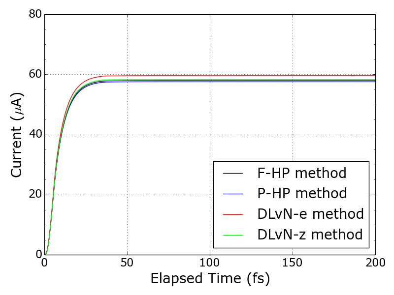
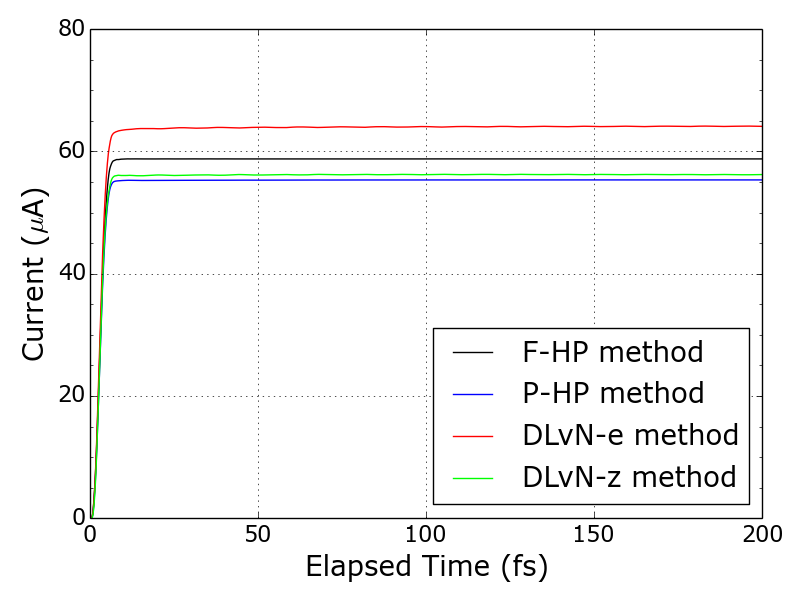
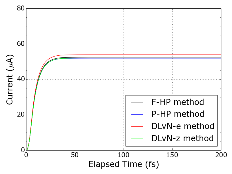
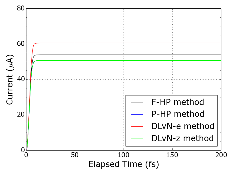
Figure 2: Current as a function of time obtained for a bias of 1.5 V with the three different implementations of the hairy-probes method (including the so called DLvN-e, given by equation 4), and with the Driven Liouville-von Neumann formula given in equation 3 (DLvN-z). The upper, middle and lower panels, correspond to the ballistic, the disordered, and the resonant models, respectively. Left and right panels show the currents for $\Gamma$ equal to 0.1 eV and 0.6 eV.

Figure 3 presents the steady state current-voltage curves obtained from the three methods deriving from HP. For the ballistic system all three approaches show only marginal differences between each other, which become negligible in the low bias region. The same is true for the disordered case. In both kinds of model system, the differences in the steady-state currents resulting from the three methods are below 5%, and typically much less than this at low biases. Somehow curiously, the scheme based on the step-potential reproduces more accurately the response of the full HP method, despite the difference in their reference densities. This suggests the existence of a compensation mechanism through which the step-generated reference density matrix balances the absence of the $\hat{\Omega}$ contribution. A possible explanation can be found in its higher polarization, as discussed below.

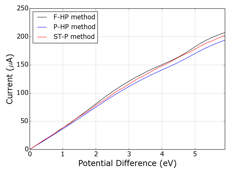
Figure 3: Current as a function of the applied bias, computed in the steady state from quantum dynamics simulations based on the three different implementations of the hairy-probes method. Results are shown for the ballistic (top), disordered (center), and resonant (bottom) model systems.

The $I-V$ curves in the resonant system display a more complex behavior. The P-HP and ST-P equations of motion still reproduce the currents of the full HP method, but with slightly larger deviations. Here, these appear to be comparable in the P-HP and in the ST-P method. The latter scheme produces in all three systems, for a given bias, higher currents than the first one. This trend was confirmed also in exploratory calculations for other resonant systems with variable separation between atoms: the step-potential yields systematically larger steady states currents than the P-HP method for a fixed potential difference. This might be related to the fact that in the case of a reference density generated from an abrupt step-field, the device is subject to a larger effective bias than in the case of a smoother reference density constructed from the Green’s functions. In other words, the action of the field, through the direct modification of the on-site energies, affects more severely the density matrix of the electrodes when compared to the HP method, in which the electrochemical potential at the leads is controlled via the coupling with external probes according to $\gamma$. This is consistent with the eigenstates populations plotted in Figure 4. The full and the P-HP simulations produce a manifold of partially occupied states, both methods exhibiting essentially no differences from each other. When the reference density derives from the step-wise potential, instead, the eigenvalues of the density matrix are 0 or 1, with a small fraction of states associated with intermediate occupations. This circumstance reflects a lower electronic temperature and a more drastic polarization in the ST-P approach arising from a highly perturbed $\hat{\rho}^{0}$, in comparison with the other two treatments. On the other hand, in the former there are a few states that violate the Pauli’s principle, bearing negative, or larger than unity occupations. The results in Figure 4 correspond to the resonant system, but analogous behavior is found for the ballistic and resonant models. The behavior of the eigenvalues for the different schemes, including the one in equation 3, is further discussed in the final section.

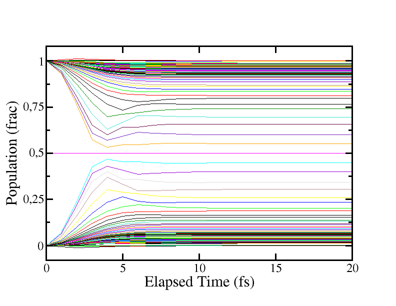
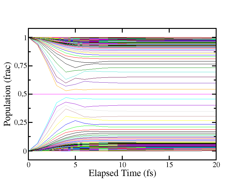
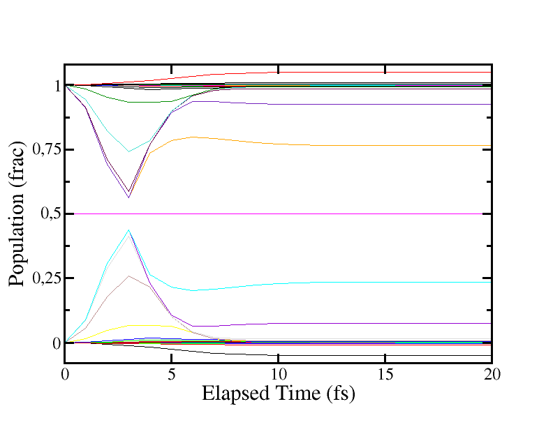
Figure 4: Temporal evolution of the eigenvalues of the density matrix for the resonant model system, computed using the full HP (top), P-HP (center), and ST-P (bottom) methods.

5 Effect of the $\Gamma$ parameter

The question of the proper value of $\Gamma$ is an interesting problem that has been investigated recently,²⁶ but has not been entirely settled. In the context of the DLvN approach, it has been argued in the literature that the magnitude of the driving rate should be somewhere between the energy spacing separating the lead levels, and the effective device-lead coupling. ²⁰ If $\Gamma$ is too high, the target density is enforced in the lead sections too tightly to allow for an appropriate response and relaxation at the interface. As a consequence, in this regime the current is a decreasing function of $\Gamma$ (see e.g. refs.  ²⁰ ,  ¹⁶ ,  ²²). Moreover, when $\Gamma$ is too low, the relaxation process in the leads is not sufficiently fast to allow for the electronic density in the leads to reach $\hat{\rho}^{0}$. The net effect in this case can be assimilated to a situation in which the leads are disconnected or weakly connected to the reservoirs and the system approaches a microcanonical regime.

On the other hand, in the context of hairy probes $\Gamma$ depends on the system parameters $d$ and $\gamma$, where $d$ is the probe surface density of states and $\gamma$ the matrix element coupling the sites at the electrodes with the external probes. While the value of $d$ can be defined to fit the density of states of the device, there is no particular criterion to uniquely assign the value of $\gamma$. In principle, in the wideband limit it is expected to satisfy the second requirement listed above for $\Gamma$ in DLvN: it must be larger than the mean energy level spacing in the leads, to ensure an effective broadening of the electronic states and hence a metallic behavior of the electrodes. In the present case this implies a lower bound for $\Gamma$ of around 0.1 eV.

Figure 5 illustrates the effect of $\Gamma$ on the $I-V$ plots in the case of the resonant system, also showing the derivatives of the current (conductance) in the insets. We chose this system because in its case the $I-V$ curve displays a distinctive physical pattern, and the discrepancies between the three approaches are more significant than in any other model, both facts making improvements easier to identify. Indeed, these discrepancies tend to fade away as $\Gamma$ decreases from 0.6 to 0.1 eV (within this range $\Gamma$ remains larger than the mean energy level spacing in the leads, of 0.078 eV). Interestingly, the insets reveal that conductances derived from the ST-P methodology turn out to be more rugged than in the other methods. This can be attributed to the presence of the self-energy in the Green’s functions, that, provided $\Gamma$ is larger than the energy level spacing in the electrodes, screens the far ends of the system in the case of the F-HP and P-HP methods. In the absence of the self-energy, finite size effects manifest in the form of interference oscillations. As a matter of fact, for a small $\Gamma$ the wiggles are visible in all three curves (see the inset on the right panel of Figure 5), because the screening effect dilutes as the Green’s function carries a dependence on this parameter in the denominator. The insets also reveal that a large $\Gamma$ value tends to damp the resonances in the ST-P case, which are otherwise intact for $\Gamma$ = 0.1 eV.

The currents obtained for a bias of 1.5 V are depicted as a function of $\Gamma$ in Figure 6, where it can be seen that the agreement between methods is progressive as the parameter gets smaller. Additionally, this Figure shows that all approaches are relatively robust against the variation of $\Gamma$, in particular the full HP scheme, for which the change in the steady state current is just 2% when this parameter is reduced by a factor of six.

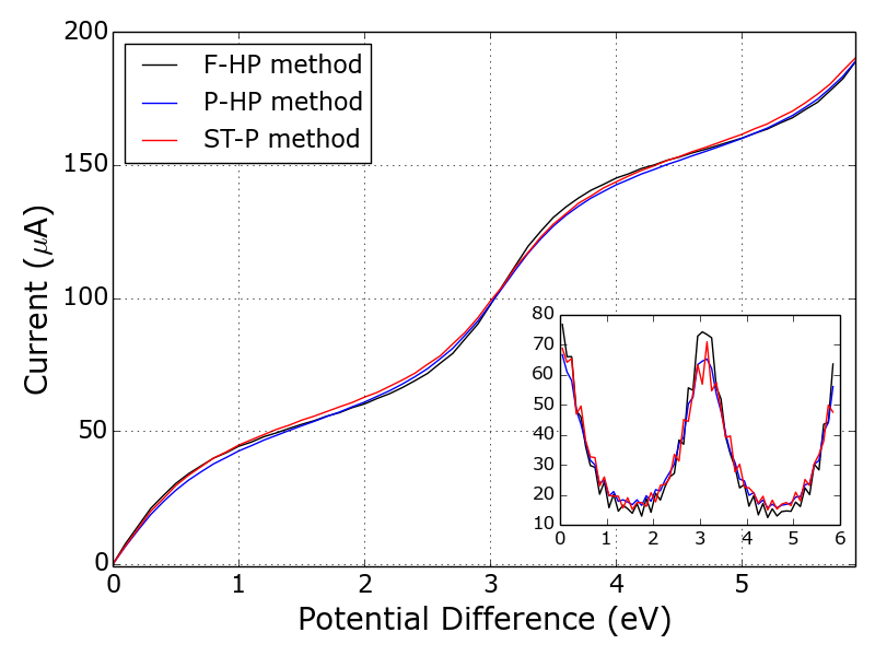
Figure 5: Steady state current as a function of the applied bias computed with the three different implementations of the hairy-probes method, for two different values of the $\Gamma$ parameter: 0.6 eV (left panel) and 0.1 eV (right panel). The results correspond to the resonant system. For a better comparison, the derivatives are shown in the insets.

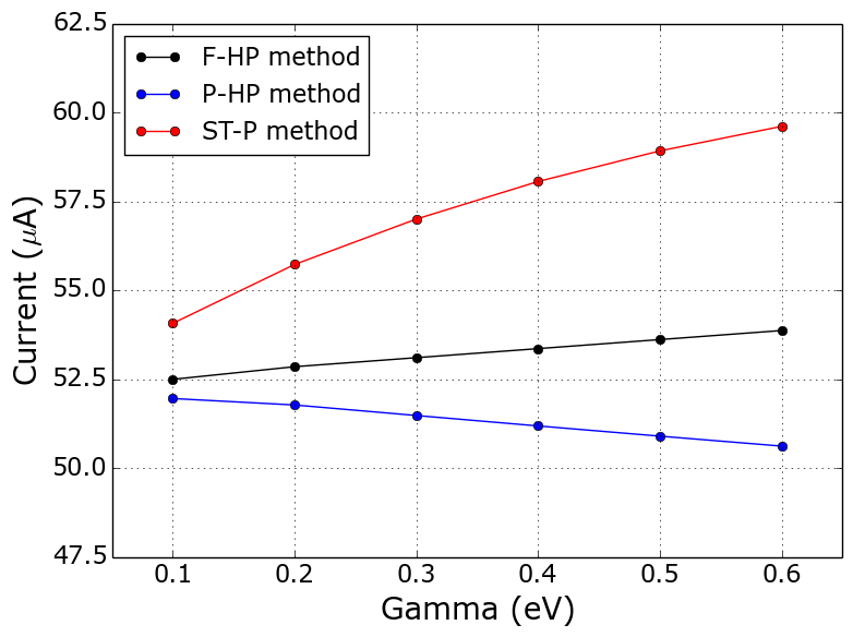
Figure 6: Steady state current as a function of the $\Gamma$ parameter, computed with the three different implementations of the hairy-probes method. The shown results correspond to the resonant system with an applied bias of 1.5 V.

In the F-HP and P-HP dynamics, the effect of $\Gamma$ arises not only from the multiplication of the driving terms, but also because the reference matrices $\hat{\rho}^{0}$ and $\hat{\Omega}$ are all functions of $\Gamma$ through the self-energy and the Green’s function (see equations 6 and 8). Therefore, it becomes relevant to check how the structure of these matrices change when varying the value of $\Gamma$. Figures 7 and 8 show that the elements of these matrices exhibit a slight inverse dependence on $\Gamma$, which, as mentioned above, limits the spatial range of the Green’s functions and reference density matrices in the electrode region, in a way that has no analogue in ST-P. This spatial damping is visible on Figures 7 and 8.

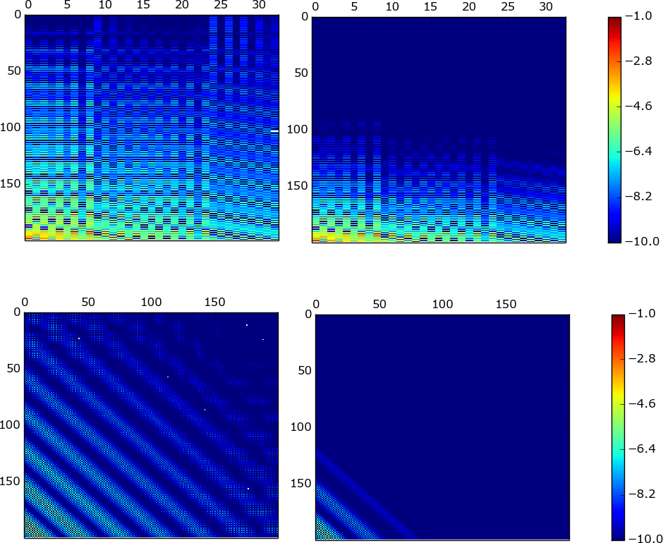
Figure 7: Color maps representing the structure of different blocks of the $\hat{\Omega}$ matrix for different values of the $\Gamma$ parameter, computed for the resonant system. Top panels: LC blocks. Bottom panels: LR blocks. Left panels: $\Gamma$=0.1 eV. Right panels: $\Gamma$=0.6 eV. The colors reflect the absolute values of the matrix elements, in a natural logarithmic scale. This matrix determines the difference between the F-HP and P-HP schemes.

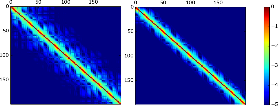
Figure 8: Color maps representing the LL block of the reference density matrix $\hat{\rho}^{0}$ in the F-HP and P-HP methods, for different values of the $\Gamma$ parameter, in the case of the resonant system. Left panel: $\Gamma$=0.1 eV. Right panel: $\Gamma$=0.6 eV. The colors reflect the absolute values of the matrix elements, in a natural logarithmic scale.

In particular, the magnitude of the $\hat{\Omega}$ contribution is responsible for the difference between the F-HP and P-HP methods. All diagonal blocks of the $\hat{\Omega}$ matrix are identically zero, and hence only the LC and LR blocks are depicted in Figure 7 (the remaining blocks, CL, RL, RC and CR are similar). The off-diagonal elements of $\hat{\Omega}$ are of the same order of magnitude as those of the reference matrix $\hat{\rho}^{0}$. Yet, the impact of the former matrix on the dynamics is only secondary because it has zeros throughout its diagonal blocks, which is where $\hat{\rho}^{0}$ gives the highest contribution. In spite of its seemingly small importance in numerical terms, though, the presence of the $\hat{\Omega}$ matrix appears to balance the effect of $\hat{\rho}^{0}$ in the current, furnishing the full HP method with a reduced sensitivity with respect to $\Gamma$.

Figure 9 displays the difference between the reference density matrices in the P-HP and ST-P methods. Given that in the latter this matrix is independent of $\Gamma$, Figure 9 just reflects the effect of this parameter on the hairy probes reference density. Interestingly, since the decrease of $\Gamma$ tends to relax the spatial damping of the P-HP reference density, which is in any case absent from the step-field generated $\hat{\rho}^{0}$, both matrices become with such a decrease more similar to each other. The agreement between these two approaches at low $\Gamma$ is manifest in the behavior of the currents in Figures 5 and 6.

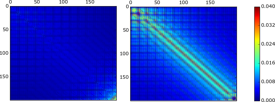
Figure 9: Color maps representing the LL block for the difference between the reference density matrices of the P-HP and ST-P methods, for the resonant system and different values of the $\Gamma$ parameter. Left panel: $\Gamma$=0.1 eV. Right panel: $\Gamma$=0.6 eV. The colors reflect the absolute values of the matrix elements.

As mentioned in the introduction, Zelovich and co-workers proposed a method for the computation of a set of broadening factors that are applied to the lead states. In this way, the rate parameter $\Gamma$ is replaced by diagonal matrices $\hat{\Gamma}_{L}$ and $\hat{\Gamma}_{R}$, with dimensions given by the number of basis sets associated with the leads. The calculation of these matrices involves a self-consistent procedure to extract from the self-energy of the isolated lead, the broadening factors that afterwards must be assigned to the corresponding levels of the lead coupled to the reservoir. Whereas this procedure is somehow involved, the $\hat{\Gamma}$ matrices are transferable to any calculation using the same lead model, and the propagation of the dynamics represents a negligible additional computational cost. The authors rationalized the magnitude of the resulting broadening factors $\Gamma_{i}$ by invoking Fermi’s golden rule for a single lead level coupled to a reservoir, which gives a value determined essentially by the coupling matrix element between lead and reservoir states. This is precisely the meaning of $\gamma$ in the context of hairy probes. In any case, this treatment was shown to be of importance in particular when the DOS of the leads is inhomogeneous in the vicinity of the Fermi energy. However, the effect of considering a single rate parameter instead of one per level was shown negligible in simple tight-binding models as the present one, where the DOS is uniform around the Fermi energy. As a matter of fact, the authors reported that the adoption of the maximal broadening value calculated for such systems using their procedure as the single driving rate, produces current traces and steady-state occupations almost indistinguishable from those obtained using the parameter-free DLvN method.

6 Generation of the reference density

The encouraging results obtained with the ST-P implementation raise the question of whether it is possible to better reproduce the F-HP dynamics with a truncated equation of motion, through the optimization of the reference density. This pathway is considered in the present section, using the shape of the electric field as a tool to prepare $\hat{\rho}^{0}$, although other strategies could be adopted as for example the state representation of Hod and co-workers. ¹⁶

We initially compare the results obtained with a step-like potential, with those corresponding to a ramp, a sigmoidal decay, and a double sigmoidal decay at the start and the end of the central region. These different patterns are illustrated in Figure 10. The analysis of the reference matrices generated in this way did not reveal any significant improvement in the description of the full hairy probes density, with the exception of a very slight increase in similarity for those matrix elements lying in the proximity of the central region. This improvement was most noticeable in the case of the sigmoid field (denoted as “SI-P”), as can be visualized in Figure 11.

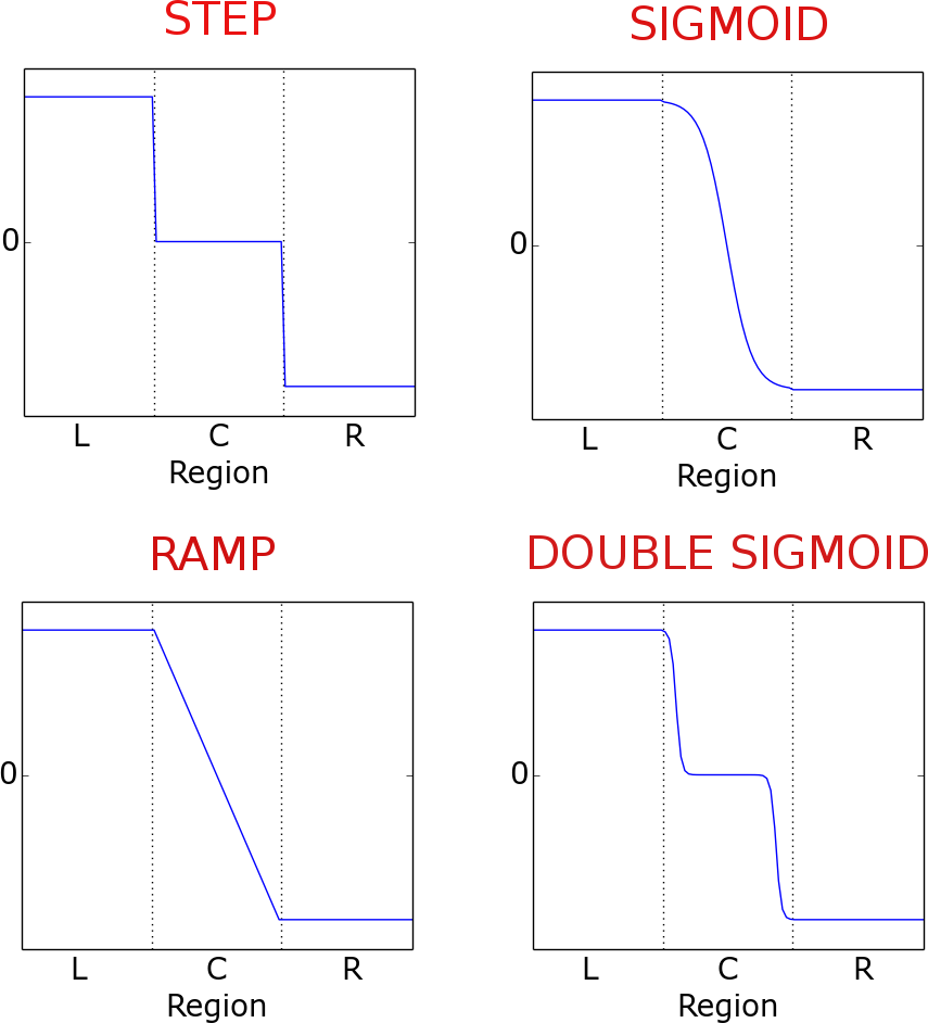
Figure 10: Shapes of the different electric fields applied to generate the reference density. L, C, and R, represent the left electrode, central, and right electrode regions, respectively.

Figure 11: Color maps representing the LL block for the difference between the reference density matrix of the full HP method with the one generated with a step field (left), or the one generated with a sigmoidal field (right). Data corresponding to the resonant system for $\Gamma$=0.6 eV. The colors reflect the absolute values of the matrix elements.

As a matter of fact, the adoption of the sigmoidal field proved to be at least as good as the step potential, when not better, to reproduce the $I-V$ plots. Figure 12 presents these curves for three resonant systems exhibiting different morphologies. Aside from the original structure displayed in Figure 1, two other models were examined in which the number of atoms in either the central or the lateral segments was extended. The value of $\Gamma$ was fixed to 0.6 eV, for which the disagreement between methods was most noticeable. For the standard resonant system the performances obtained from the step or the sigmoidal potentials are comparable. The same is true for the alternative resonant model with a longer intermediate region, for which no significant differences are found between the results yielded by either method. However, in this case the description provided by these two approaches is manifestly worse. In this sense, it is noteworthy that the P-HP scheme is still able to capture the main features of the full hairy probes curve. On the other hand, in the third model where the device bears longer lateral segments, the reference calculated with the sigmoidal potential outperforms the one calculated with the step-like field.

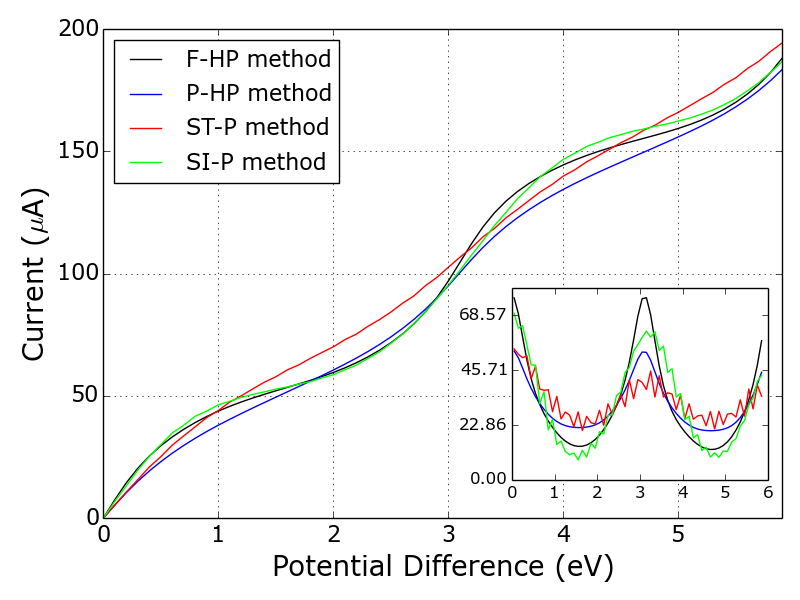
Figure 12: Steady state currents as a function of the applied potential, computed with different implementations of the hairy-probes method with $\Gamma$ = 0.6 eV. Results are shown for the resonant system with different arrangements of the atoms in the central region: 9-15-9 (top), 9-45-9 (center), and 30-15-30 (bottom).

7 The two different forms of the Driven Liouville-von Neumann formula

Equations 3 and 4 are two expressions of the DLvN approach, both of which had an heuristic origin, and for which different formal derivation routes have been proposed. From a mathematical point of view, the difference between these two formulas is found in the off-diagonal elements of the driving term: while in equation 3 these damp the lead-device coherences to zero, in equation 4 coherences are pushed towards their equilibrium values. Their derivations involve different approximations and assumptions, and it is of particular interest to compare the paths that lead to one or the other. This is the goal of the present section, where the performances of the two schemes are also confronted.

It is possible to identify three assumptions or approximations specific to one or the other formula, that explain their different mathematical structures:

1. In equation 3, the explicit lead levels are in contact with an implicit fermionic reservoir, for which coupling the wideband limit is assumed. Equation 4 is in turn a truncation of the hairy probes formula, where the leads are coupled to a set of probes in which the wideband limit holds. The latter procedure broadens but preserves the electronic structure of the (finite) leads adjoining the central region.

2. To arrive to DLVN-z, it is assumed that the relaxation dynamics in the leads is independent of the presence of the device. This amounts to the zeroth-order approximation of the Green’s functions in which $G^{adv}$ and $G^{ret}$ commute with the leads subspace projector $Q$. This step eventually leads to the disappearence of $\rho^{eq}$ in the last term of equation 36 in the work by Franco et al.²⁰ Interestingly, the same result would also be obtained e.g. from equations 15 or 16 of our manuscript, if $\hat{P}_{L}$ or $\hat{P}_{R}$ were assumed to commute with the Green’s functions $\hat{G}^{\pm}_{S}$. In such a case, these contributions would vanish, suppressing $\rho^{0L}$ and $\rho^{0R}$ from the off-diagonal elements of the equation of motion, and thus giving rise to a driving term analogous to DLvN-z. Thus, the damping of the coherences either to zero or to equilibrium is related to this approximation in the Green’s functions, which physically translates into an independency of the electron dynamics in the leads with respect to the device.

3. Finally, the $\hat{\Omega}$ terms are dropped from the HP expression to arrive at DLvN-e. These terms arise from the Green’s functions keeping track of the forward time-propagation of carriers coming from the probes. Thus, they introduce a propagation sense to the injected lead-device charge. Its suppression must imply a drop in the current, as is certainly observed in the simulations.

In ref. ²²   it has been reasoned that while DLvN-z represents a device between electronic reservoirs at equilibrium with well-defined chemical potentials, DLvN-e resembles the state of a charged capacitor, where the target density represents the equilibrium state of the entire finite junction model and not just the leads. This seems to be consistent with the origins of each of these schemes, that have now come to light. Figure 13 depicts the current-voltage curves for the two DLvN approaches, together with the results of the HP method. At small couplings it can be seen that the performance of any of these methods is essentially indistinguishable from each other. As the $\Gamma$ parameter is increased, discrepancies start to emerge.

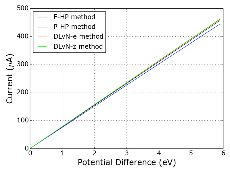
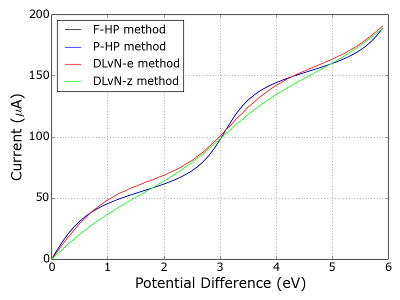
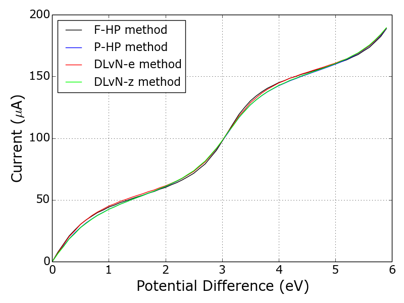
Figure 13: Steady state current as a function of the applied bias computed with the two forms of the DLvN equation and with the hairy-probes method. The top panel presents the data corresponding to the ballistic (left) and disordered (right) systems, for $\Gamma$ equal to 0.6 eV. The bottom panel shows the results for the resonant system with $\Gamma$ equal to 0.6 eV (left) and 0.1 eV (right).

DLvN-z has been shown to observe Pauli’s principle regardless of the initial conditions.¹⁶ It is interesting to note that, while the hairy probes scheme also fulfills Pauli’s principle at long times (by construction), it does not necessarily obey it in the transient. This can be seen in Figure 14, which displays the occupations for F-HP, P-HP, DLvN-e, and DLvN-z in the resonant system. It must be recalled that in all these schemes, the dynamics is switched on smoothly, to avoid sudden jumps which could lead to numerical discontinuities. Specifically, the driving term and the $\Omega$ term are introduced in the first part of the simulation using a linear ramp. For F-HP, the positive and negative deviations from 1 and 0 respectively—which become smaller with a smoother ramp—disappear in the long term. When the $\Omega$ term is suppressed from the F-HP scheme, the dynamics and in particular the occupations are affected but the exclusion principle is still obeyed in the steady state. However, if the reference density matrix is replaced by the one obtained from an electric field to give the DLvN-e approach, the violation to the exclusion principle persists even in the steady state. This is not observed with the DLvN-z method, for which the exclusion principle is satisfied throughout the full dynamics, despite the adoption of the same $\hat{\rho}^{0}$ as in DLvN-e. Interestingly, this makes manifest that the observance of Pauli’s principle is determined neither by $\Omega$ nor by the reference density, but by their combination.

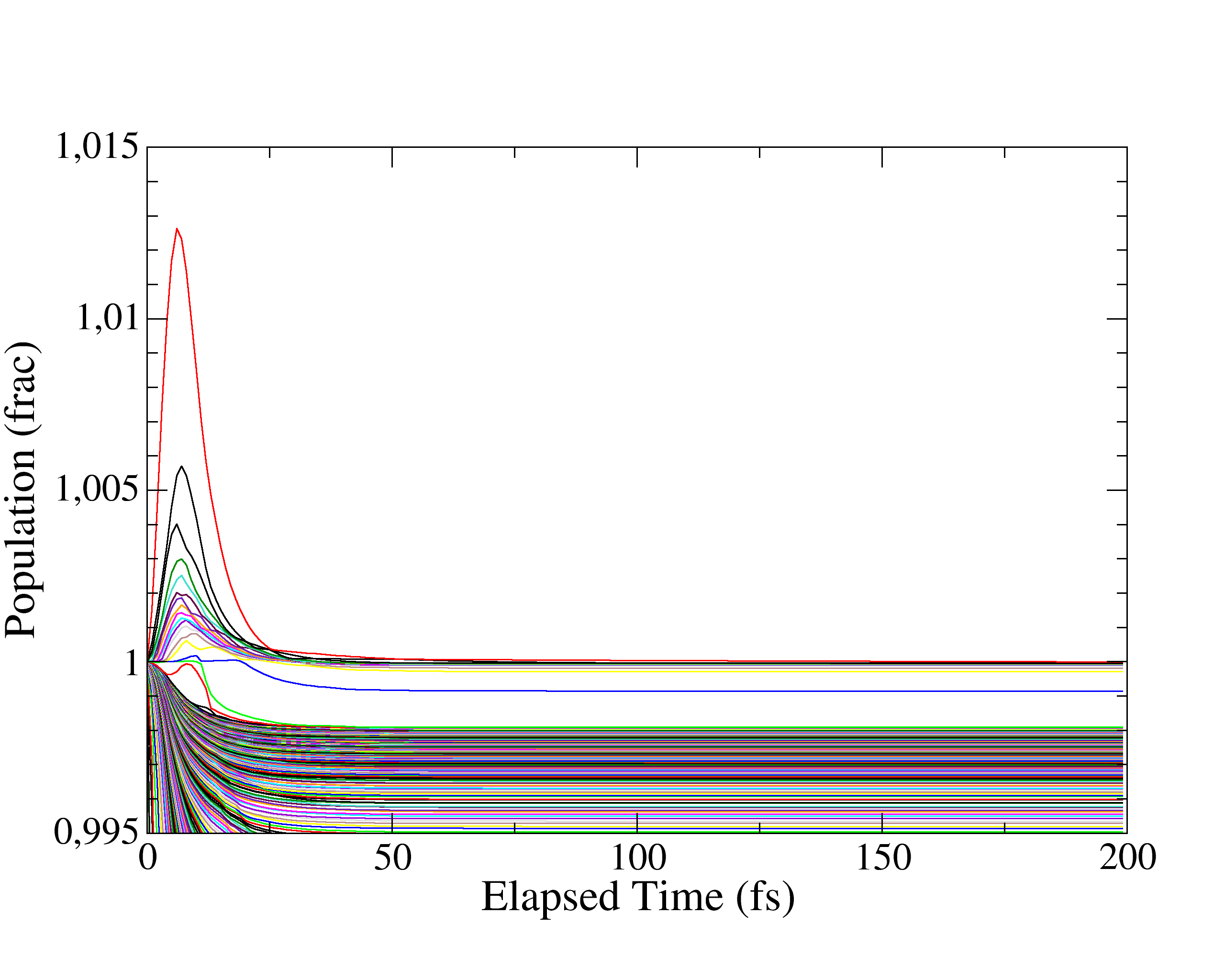
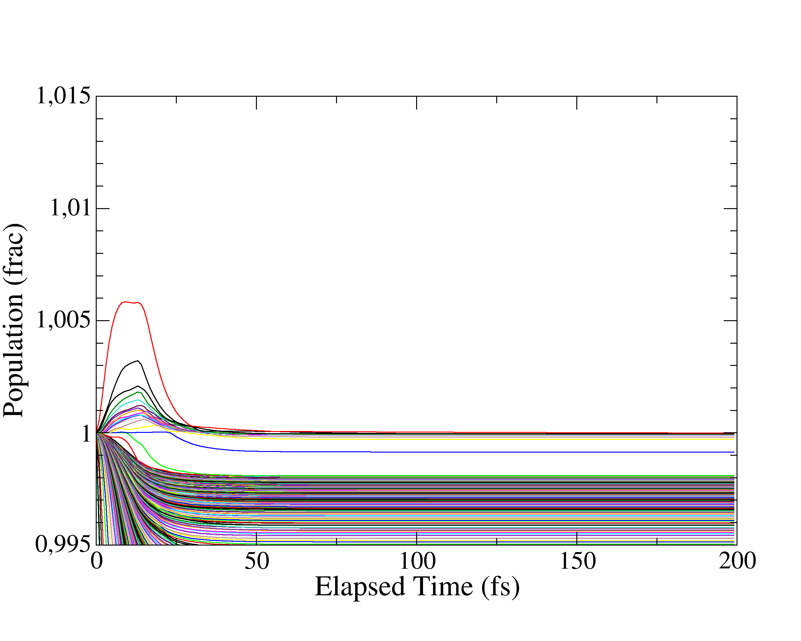
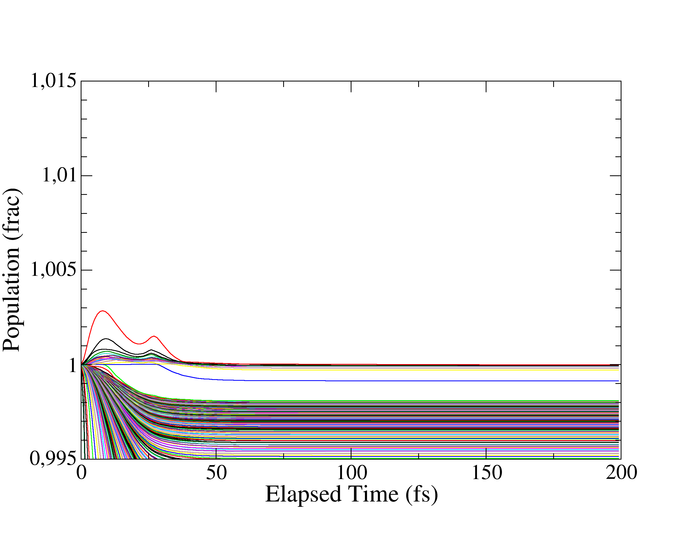
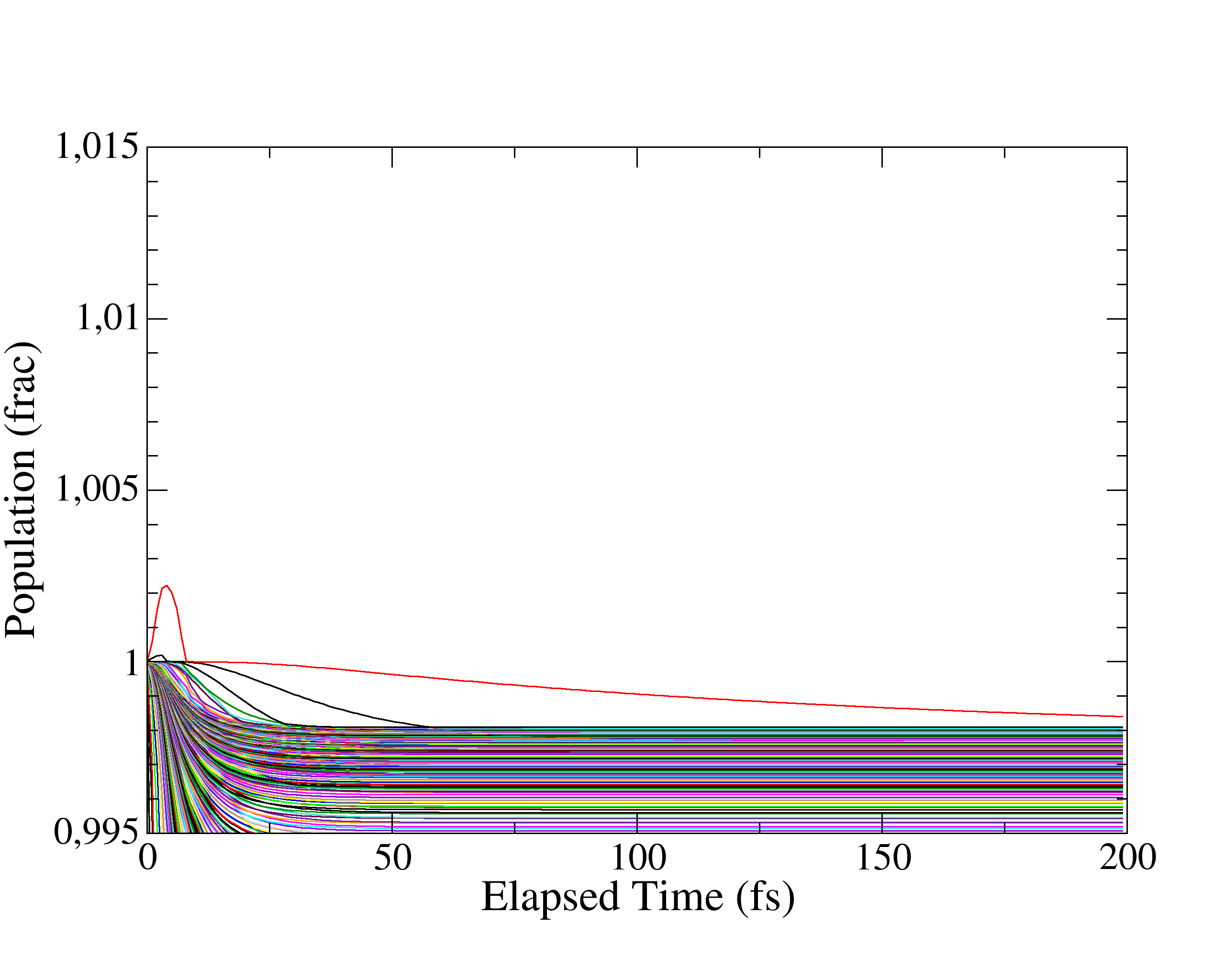
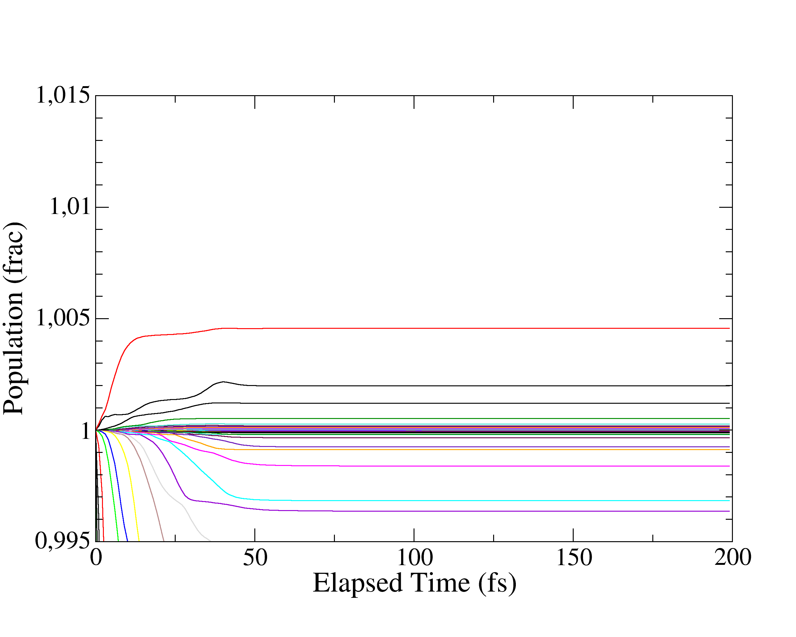
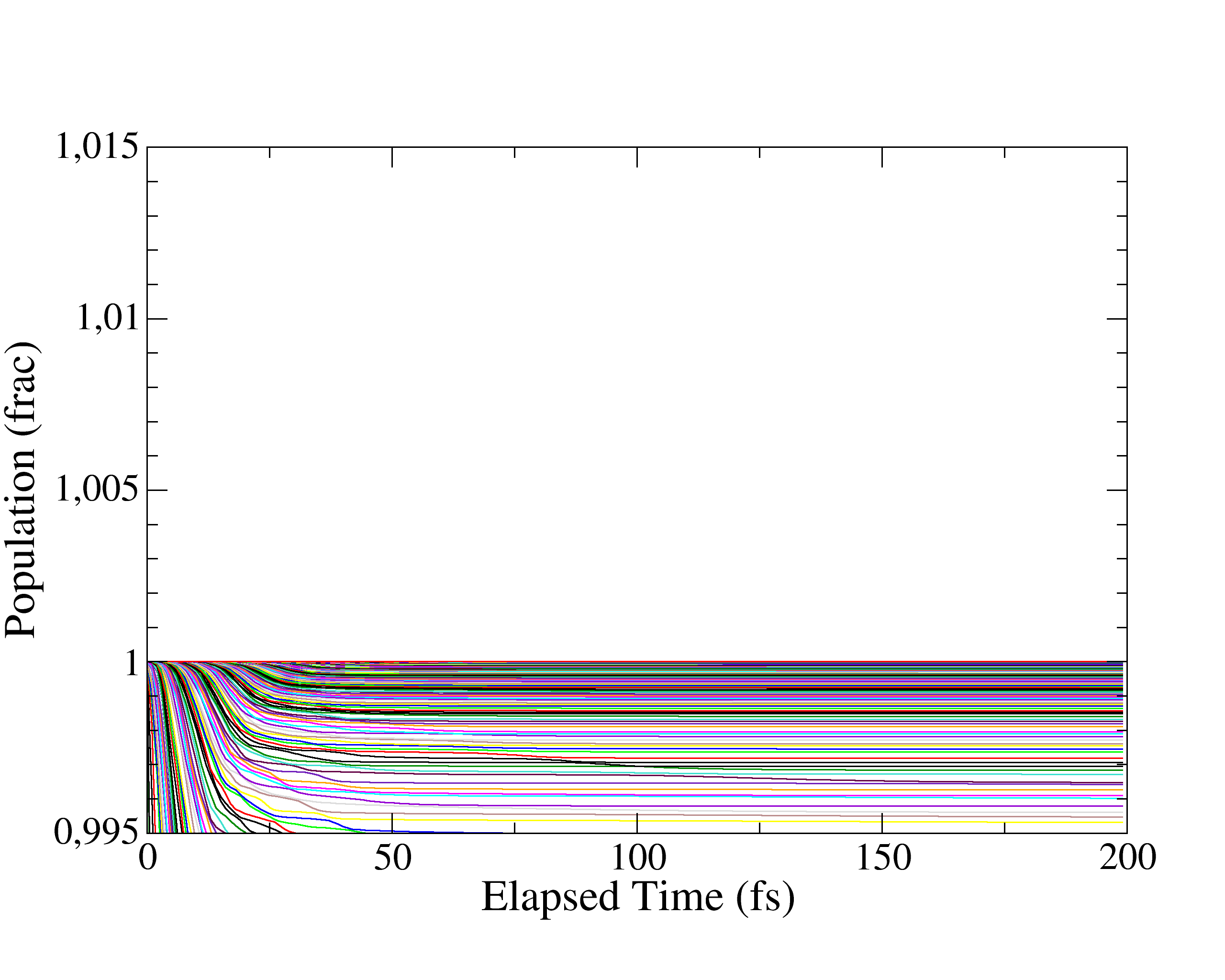
Figure 14: Temporal evolution of the eigenvalues of the density matrix for the resonant model system. The top row corresponds to the full HP method where the driving term was appplied gradually using ramps of different durations: 5.0 fs, 12.5 fs and 25.0 fs (from left to right). The bottom row compares the behavior found with the other methods using a ramp of 5.0 fs: the P-HP (left), the DLvN-e (center) and the DLvN-z (right) schemes. Part of this data has been already given in a different size scale in Figure 4.

Finally, Figure 15 explores the effect of $\Gamma$ and of the electrode size on the currents, using the resonant model. The bottom left panel shows that the HP method, consistently with its physical origin, is particularly robust with respect to electrode size and $\Gamma$. In the case of an electrode of 50 atoms, significant deviations in the current are observed only for $\Gamma<$0.2 eV. The two upper panels depict the I-V curves for the DLvN-e and DLvN-z approaches, compared with the F-HP method. In both cases it can be observed that the reduction of the electrode size to 50 atoms affects the currents. The agreement with F-HP improves marginally as $\Gamma$ decreases, until it breaks down when this parameter falls below the wideband limit, which in this case is higher since the energy level spacing becomes larger with smaller leads. This distortion in the currents is less critical in the DLvN-e approach. In particular, the bottom right panel displays the difference between the benchmark F-HP current ($\Gamma$=0.6 eV, 200 atoms in the leads) and the currents produced by the DLvN approaches ($\Gamma$=0.3 and 50 atoms in the leads). It can be seen that deviations tend to be larger for DLvN-z, whereas the DLvN-e approach, inheriting the mathematical structure from F-HP, copes better with the shortening of the electrodes.

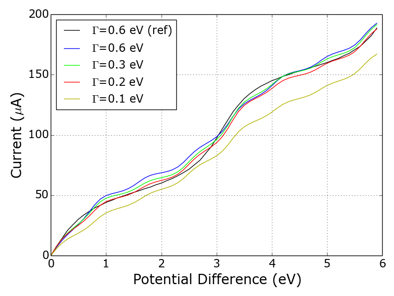
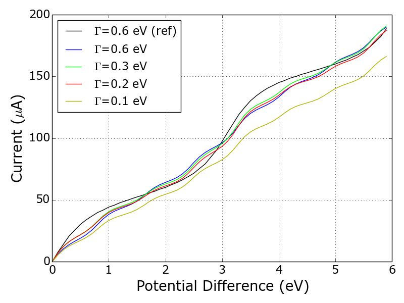
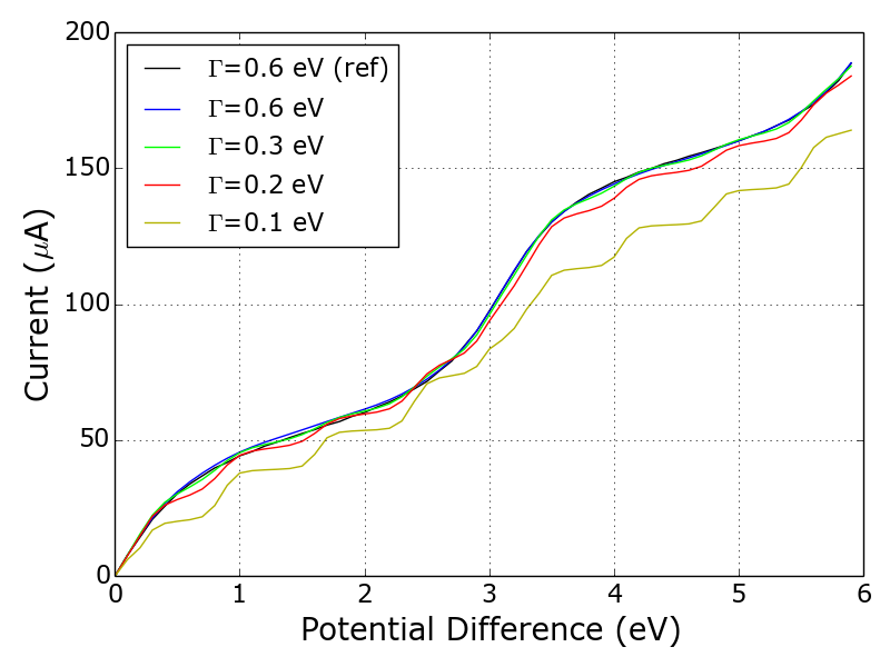
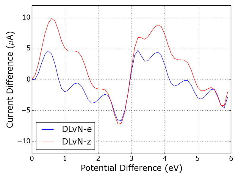
Figure 15: Effect of electrode size and of the $\Gamma$ parameter on the current-voltage curves obtained for the resonant model. Top panels present in black the curve obtained from F-HP with 200 atoms in each lead and $\Gamma$=0.6 eV (labelled ref), in comparison with the curves computed using 50 atoms leads and different $\Gamma$ values for the DLvN-e (left) and DLvN-z (right) methods. We also include the behaviour of the F-HP method with the small electrodes and varying $\Gamma$ (bottom left). The bottom right panel displays, for DLvN-e and DLvN-z ($\Gamma$ = 0.3 eV), the difference with respect to the F-HP current (obtained with $\Gamma$ = 0.6 eV).

To summarize, the two forms of the Driven Liouville-von Neumann equation produce similar results, reproducing the hairy probes method provided large values of $\Gamma$ are avoided. The most noticeable difference is that, whereas DLvN-z observes Pauli’s principle, DLvN-e does not. At the same time, in some situations the DLvN-e equation is more tolerant to a decrease of electrode size, as discussed in ref.²²  , which is a consequence of the robustness of the HP method from which it is descended.

8 Summary and final remarks

In this article, it was shown that the Green’s functions based multiple-probes—or hairy probes—formalism, adopts a form equivalent to the heuristic Driven Liouville-von Neumann method as proposed in reference  ²² (equation 4), plus an additional term involving a matrix ($\hat{\Omega}$) with null diagonal blocks. A distinctive feature of this form of the DLvN equation of motion is that, at variance with the previous versions introduced in references  ¹³  or  ¹⁶ , the coherences are damped to the equilibrium density. It has been argued that in this approach the electrodes are not meant to represent infinite reservoirs with homogeneous and well defined chemical potentials. Instead, through the action of the driving operator, the leads are driven close to, rather than exactly to, the target density.²² This is parallel to the physics in the HP model, where the electrodes are connected to multi-probes with electrochemical potentials $\mu_{L/R}$. The electrochemical potential of the lead is not necessarily that of the probes but depends on the strength of their coupling (and on position down the lead). These particular boundary conditions of the HP method are reminiscent of those in the DLvN implementation of equation 4 and demonstrated to be well suited for small size electrodes.²²

To neglect the $\hat{\Omega}$ matrix in the driving term of the HP formula has minor effects on the dynamics and the steady state currents obtained for a variety of model systems. These effects are even less significant when the coupling between the probes and the leads is reduced by decreasing the $\Gamma$ parameter. More specifically, our results show that the P-HP method can reproduce the behavior described by the full HP scheme for ballistic and disordered systems, and with some care it can also be tuned for more complicated resonant systems. In general, at least in the context of tight-binding Hamiltonians, it is possible to conclude that the DLvN method, incarnated here in the P-HP or ST-P equations of motion, converges to the hairy probes description in the limit of small couplings between the probes and the leads (providing $\Gamma$ is still larger than the energy level spacing). The P-HP method can be thought of as a version of the DLvN approach in which the calculation of the reference density is based on Green’s functions. The ST-P method, on the other hand, reproduces the formulation presented in reference  ²² . It has proved to be a very good approximation to the full HP description, but the finite size effects which manifest in the absence of a self-energy imply a limitation in comparison with the P-HP approach that seems difficult to overcome.

The possibility to avoid the calculation of Green’s functions acquires special interest for the applications in the context of TDDFT or other first-principles schemes. In that respect, we explored the substitution of the reference density computed from Green’s functions in the P-HP method, by the one emerging from an electric field applied to the system. This strategy systematically produced higher currents than the P-HP method, presumably because the application of a field, in the present setting, amounts to an additive constant in the density matrix elements, whereas in the HP scheme the chemical potential is fixed at an external probe and not directly on the leads, whose polarization is mediated by a coupling parameter. The effective bias arising between the electrodes in operation conditions may thus not be as large as the one imposed by the field. Further sources of improvement for the region-weighted field-generated reference density method proved hard to find. Our results here seem to suggest that the step and sigmoideal shapes fields can better fit those parts of the reference matrices at the boundary with the device, providing the most accurate representations of the current in comparison with the other fields tested. Whereas the ballistic and disordered models could be described reasonably well with the ST-P and SI-P schemes, the resonant systems proved to be challenging for those methods using electric-field based reference densities. This limitation becomes particularly relevant for TDDFT applications, where the complexity of the chemical structures, far from the simple tight-binding models examined in the present work, may lead to stronger discrepancies between the results obtained using a reference density generated from Green’s functions or from an electric field. It would be interesting to establish how the different reference densities and the omission of the $\hat{\Omega}$ matrix affect the dynamics in the case of first-principles simulations. That question will be the subject of future work.

This work was supported by a research grant from Science Foundation Ireland (SFI) and the Department for the Economy Northern Ireland under the SFI-DfE Investigators Programme Partnership, Grant Number 15/IA/3160, by the Argentinean Agency for Scientific and Technological Promotion (ANPCYT) through PICT 2015-2761, and by the University of Buenos Aires, UBACYT 20020160100124BA. We are grateful to Uriel Morzan for very appreciated discussions.

References

- Landauer 1957 Landauer, R. Spatial Variation of Currents and Fields Due to Localized Scatterers in Metallic Conduction. IBM J. Res. Dev. 1957, 1, 223–231
- Buttiker 1986 Buttiker, M. Four-Terminal Phase-Coherent Conductance. Phys. Rev. Lett. 1986, 57, 1761
- Brandbyge et al. 2002 Brandbyge, M.; Mozos, J.-L.; Ordejón, P.; Taylor, J.; Stokbro, K. Density-Functional Method for Nonequilibrium Electron Transport. Phys. Rev. B 2002, 65, 165401
- Kosov 2004 Kosov, D. S. Lagrange Multiplier Based Transport Theory for Quantum Wires. J. Chem. Phys. 2004, 120, 7165–7168
- Goyer et al. 2007 Goyer, F.; Ernzerhof, M.; Zhuang, M. Source and Sink Potentials for the Description of Open Systems with a Stationary Current Passing Through. J. Chem. Phys. 2007, 126, 144104
- Koentopp et al. 2008 Koentopp, M.; Chang, C.; Burke, K.; Car, R. Density Functional Calculations of Nanoscale Conductance. J. Phys-Condens. Mat. 2008, 20, 083203
- Thoss and Evers 2018 Thoss, M.; Evers, F. Perspective: Theory of Quantum Transport in Molecular Junctions. J. Chem. Phys. 2018, 148, 030901
- Kurth et al. 2005 Kurth, S.; Stefanucci, G.; Almbladh, C.-O.; Rubio, A.; Gross, E. K. U. Time-Dependent Quantum Transport: A Practical Scheme Using Density Functional Theory. Phys. Rev. B 2005, 72, 035308
- Burke et al. 2005 Burke, K.; Car, R.; Gebauer, R. Density Functional Theory of the Electrical Conductivity of Molecular Devices. Phys. Rev. Lett. 2005, 94, 146803
- McEniry et al. 2007 McEniry, E. J.; Bowler, D. R.; Dundas, D.; Horsfield, A. P.; Sánchez, C. G.; Todorov, T. N. Dynamical Simulation of Inelastic Quantum Transport. J. Phys-Condens. Mat. 2007, 19, 196201
- Mühlbacher and Rabani 2008 Mühlbacher, L.; Rabani, E. Real-Time Path Integral Approach to Nonequilibrium Many-Body Quantum Systems. Phys. Rev. Lett. 2008, 100, 176403
- Horsfield et al. 2004 Horsfield, A. P.; Bowler, D.; Fisher, A. Open-boundary Ehrenfest Molecular Dynamics: Towards a Model of Current Induced Heating in Nanowires. J. Phys-Condens. Mat. 2004, 16, L65
- Sánchez et al. 2006 Sánchez, C. G.; Stamenova, M.; Sanvito, S.; Bowler, D.; Horsfield, A. P.; Todorov, T. N. Molecular Conduction: Do Time-Dependent Simulations Tell You More than the Landauer Approach? J. Chem. Phys. 2006, 124, 214708
- Subotnik et al. 2009 Subotnik, J. E.; Hansen, T.; Ratner, M. A.; Nitzan, A. Nonequilibrium Steady State Transport Via the Reduced Density Matrix Operator. J. Chem. Phys. 2009, 130, 144105
- Rothman and Mazziotti 2010 Rothman, A. E.; Mazziotti, D. A. Nonequilibrium, Steady-State Electron Transport With N-Representable Density Matrices from the Anti-Hermitian Contracted Schrödinger Equation. J. Chem. Phys. 2010, 132, 104112
- Zelovich et al. 2014 Zelovich, T.; Kronik, L.; Hod, O. State Representation Approach for Atomistic Time-Dependent Transport Calculations in Molecular Junctions. J. Chem. Theory Comput. 2014, 10, 2927–2941
- Zelovich et al. 2015 Zelovich, T.; Kronik, L.; Hod, O. Molecule-Lead Coupling at Molecular Junctions: Relation Between the Real- and State-Space Perspectives. J. Chem. Theory Comput. 2015, 11, 4861–4869
- Hod et al. 2016 Hod, O.; Rodríguez-Rosario, C. A.; Zelovich, T.; Frauenheim, T. Driven Liouville von Neumann Equation in Lindblad Form. J. Phys. Chem. A. 2016, 120, 3278–3285
- Zelovich et al. 2016 Zelovich, T.; Kronik, L.; Hod, O. Driven Liouville von Neumann Approach for Time-Dependent Electronic Transport Calculations in a Nonorthogonal Basis-Set Representation. J. Phys. Chem. C. 2016, 120, 15052–15062
- Chen et al. 2014 Chen, L.; Hansen, T.; Franco, I. Simple and Accurate Method for Time-Dependent Transport along Nanoscale Junctions. J. Phys. Chem. C 2014, 118, 20009–20017
- Zelovich et al. 2017 Zelovich, T.; Hansen, T.; Liu, Z.-F.; Neaton, J. B.; Kronik, L.; Hod, O. Parameter-Free Driven Liouville-von Neumann Approach for Time-Dependent Electronic Transport Simulations in Open Quantum Systems. J. Chem. Phys. 2017, 146, 092331
- Morzan et al. 2017 Morzan, U. N.; Ramírez, F. F.; González Lebrero, M. C.; Scherlis, D. A. Electron Transport in Real Time from First-Principles. J. Chem. Phys. 2017, 146, 044110
- Todorov 2002 Todorov, T. N. Tight-Binding Simulation of Current-Carrying Nanostructures. J. Phys-Condens. Mat. 2002, 14, 3049
- Dundas et al. 2009 Dundas, D.; McEniry, E. J.; Todorov, T. N. Current-Driven Atomic Waterwheels. Nat. Nanotechnol. 2009, 4, 99
- McEniry et al. 2010 McEniry, E.; Wang, Y.; Dundas, D.; Todorov, T.; Stella, L.; Miranda, R.; Fisher, A.; Horsfield, A.; Race, C.; Mason, D. et al. Modelling Non-Adiabatic Processes Using Correlated Electron-Ion Dynamics. Eur. Phys. J. B 2010, 77, 305–329
- Horsfield et al. 2016 Horsfield, A. P.; Boleininger, M.; D’Agosta, R.; Iyer, V.; Thong, A.; Todorov, T. N.; White, C. Efficient Simulations with Electronic Open Boundaries. Phys. Rev. B 2016, 94, 075118
- Sutton et al. 2001 Sutton, A. P.; Todorov, T. N.; Cawkwell, M. J.; Hoekstra, J. A Simple Model of Atomic Interactions in Noble Metals Based Explicitly on Electronic Structure. Philos. Mag. A 2001, 81, 1833–1848