Hubbard pair cluster with elastic interactions. Studies of thermal expansion, magnetostriction and electrostriction

Abstract

The pair cluster (dimer) is studied within the framework of the extended Hubbard model and the grand canonical ensemble. The elastic interatomic interactions and thermal vibrational energy of the atoms are taken into account. The total grand potential is constructed, from which the equation of state is derived. In equilibrium state, the deformation of cluster size, as well as its derivatives, are studied as a function of the temperature and the external magnetic and electric fields. In particular, the thermal expansion, magnetostriction and electrostriction effects are examined for arbitrary temperature, in a wide range of Hamiltonian parameters.

In Memory of Professor Leszek Wojtczak

1 Introduction

The Hubbard model [1, 2, 3, 4] plays an important role in contemporary solid state physics. Since its formulation, numerous applications of the model have been developed and the model itself has been extensively investigated as a fundamental, prototypic model for description of correlated fermions [5, 6, 7, 8]. Many of the studies were concentrated on the typical three-dimensional, two-dimensional or one-dimensional Hubbard model (e.g. [9, 10, 11]). However, with an increase of interest in studies of nanoclusters, which is stimulated by the development of nanotechnology, intensive investigations of the Hubbard model applied to the systems containing small number of atoms have been performed. Some of them involve the studies of small clusters with either exact or close to exact methods [12, 13, 14, 15, 16, 17, 18, 19, 20, 21, 22, 23, 24, 25, 26, 27, 28, 29]. Among such systems, a two-atomic cluster (dimer) plays a special role, being the smallest nanosystem where the Hubbard model can be adopted, and the exact analytical solutions can be found. As a consequence, numerous aspects of physics of Hubbard dimers focused considerable attention in the literature [30, 31, 32, 33, 34, 35, 36, 37, 38, 39, 40, 41, 42, 43, 44, 45, 46, 47, 48, 49]. These facts serve as a sound motivation for further comprehensive study of the two-atomic Hubbard system aimed at its full and exact thermodynamic description. In line with this trend, recently the Hubbard pair cluster embedded simultaneously in the external magnetic and electric fields has been studied by the exact analytical methods in the framework of the grand canonical ensemble. In this approach the system is open, so that it is able to exchange the electrons with its environment [41, 42, 43]. The statistical and thermodynamic properties, both magnetic and electric ones, have been extensively studied there.

Despite these investigations, there is still room for extending the model of interest. Supplementing purely electronic models by including further degrees of freedom can cause new kinds of behaviour to emerge and new control parameters can be gained this way. Purely electronic models can be supplemented, for example, with subsystems composed of localized spins (e.g. [50, 51, 52, 53, 54, 55, 56, 57]), which are still exactly solvable. Immersing of such system in the external fields can give access to unique properties (like, for example, manifestations of the magnetoelectric effect [56]). Enriching the purely electronic models is also a step towards more complete characterization of the real physical systems. A good example can be inclusion of the Hamiltonian terms, which are responsible for coupling of the electronic degrees of freedom with the lattice. Such a study, aimed at the description of magnetomechanical and electromechanical properties of the Hubbard dimer, has not been undertaken yet. Therefore, the aim of the present paper is extension of the recent studies, basing on the formalism developed in Ref. [41], by including elastic interactions in the description of the Hubbard dimer. Such interactions are especially important since they are responsible for stability of the dimer structure and allow to account for the energy of thermal vibrations. It can be expected that after combining with the Hubbard Hamiltonian, the elastic interactions will lead to new phenomena, connecting the magnetic, electric and mechanical properties.

The elastic interaction between the atoms is assumed here in the form of the Morse potential [58, 59]. The thermal vibrational energy is obtained in the quasi-harmonic approximation, where the anharmonicity is taken into account by the Grüneisen parameter [60, 61]. In turn, the Hubbard pair Hamiltonian is taken in its extended form, with the Coulomb interaction between the electrons on different atoms and the hopping integral depending on dimer size.

On the basis of the above assumptions, the total grand thermodynamic potential is constructed, from which all statistical and thermodynamic properties can be obtained in a self-consistent manner. In particular, the deformation of interatomic distance (dimer length), magnetostriction and electrostriction coefficients are calculated for various temperatures, and the effect of the external magnetic and electric fields on the mentioned quantities is also investigated. In addition, the chemical potential is studied in the presence of elastic interactions, showing a new behaviour in comparison with the conventional Hubbard model. A special attention is paid to the low-temperature region, where the discontinuous quantum changes of these properties can be demonstrated.

The paper is organized as follows: In the next Section the theoretical model is presented and the basic formulae, important for numerical calculations, are derived. In the successive Section the selected results of calculations are illustrated in figures and discussed. The last Section is devoted to a brief summary of the results and final conclusions.

2 Theoretical model

In the present section, a step-by-step development of the theoretical model for the Hubbard dimer including the elastic and vibrational properties is presented and the solution of the model is described.

2.1 Grand potential for the Hubbard dimer

Extended Hubbard Hamiltonian for the pair of atoms $(a,b)$ embedded in the external fields is of the form:

$$\mathcal{H}_{a,b} = -t\sum_{\sigma=\uparrow,\downarrow}\left(c_{a,\sigma}^{+}c_{b,\sigma}+c_{b,\sigma}^{+}c_{a,\sigma}\right)+U\left(n_{a,\uparrow}n_{a,\downarrow}+n_{b,\uparrow}n_{b,\downarrow}\right)$$ (1)

$$-H\left(S_{a}^{z}+S_{b}^{z}\right)-V\left(n_{a}-n_{b}\right)+Wn_{a}n_{b},$$

where $t>0$ is the hopping integral, $U\geq 0$ is on-site Coulomb repulsion and $W$ stands for the Coulomb interaction between electrons localized on $a$ and $b$ atoms. In 1, $H=-g\mu_{\rm B}H^{z}$ denotes the magnitude of an external uniform magnetic field $H^{z}$, whereas the electric field $E$ is determined by the electrostatic potentials $V_{a}=-V_{b}=V$ applied to both atoms. Thus, $E=2V/\left(|e|d\right)$, where $d$ is the interatomic distance and $e$ is the electron charge. The quantity $W$ in 1 is assumed in the classical form: $W=1/(4\pi\epsilon_{0})\,e^{2}/d$.

The creation ($c_{\gamma,\sigma}^{+}$) and annihilation ($c_{\gamma,\sigma}$) operators for site $\gamma=a,b$ and spin state $\sigma$ can be used to construct the occupation number operators $n_{\gamma,\sigma}$ for the electrons with given spin:

$$n_{\gamma,\sigma}=c_{\gamma,\sigma}^{+}c_{\gamma,\sigma}.$$ (2)

The total occupation number operators at the site $\gamma=a,b$ are then given by:

$$n_{\gamma}=n_{\gamma,\uparrow}+n_{\gamma,\downarrow}.$$ (3)

Moreover, the spin operators $S_{\gamma}^{z}$ are defined as follows:

$$S_{\gamma}^{z}=\left(n_{\gamma,\uparrow}-n_{\gamma,\downarrow}\right)/2.$$ (4)

Since we intend to study the elastic properties of the model, the interatomic distance $d$ can be presented as follows:

$$d=d_{0}\left(1+\varepsilon\right),$$ (5)

where $d_{0}$ is the equilibrium distance defined in the absence of the external fields ($H=0,\,E=0$) and for zero temperature ($T=0$). In 5, $\varepsilon$ defines the temperature and fields-induced deformation. As it can be noted, some of the coefficients in Hamiltonian 1, like $V$, $W$ and $t$, are interatomic distance-dependent. For instance, for the electric potential we have:

$$V=V_{0}\left(1+\varepsilon\right),$$ (6)

where $V_{0}=E|e|d_{0}/2$. In turn, for the interatomic Coulomb interaction we can write:

$$W=\frac{W_{0}}{1+\varepsilon},$$ (7)

where $W_{0}=\frac{e^{2}}{4\pi\epsilon_{0}d_{0}}$. Moreover, for the hopping integral we assume the power-law distance dependence, namely:

$$t=t_{0}\left(\frac{d}{d_{0}}\right)^{-n}=t_{0}\left(1+\varepsilon\right)^{-n},$$ (8)

with a constant power index $n$, which can be used if the deformation $\varepsilon$ is small.

We treat the Hubbard pair as an open system, with a variable number of electrons, which can be exchanged with the environment. It corresponds to the physical situation when, for instance, the cluster is interacting with the metallic substrate, which forms the electronic reservoir, and the average number of electrons in the system results from the thermodynamic equilibrium. In such small system the relative fluctuations of the number of electrons, when related to its statistical mean value, can be significant. Therefore, in this case a formalism of the grand canonical ensemble should be used, which is more appropriate here than the canonical ensemble, with a fixed number of electrons.

In the framework of the grand canonical ensemble, the Hamiltonian 1 should be extended by adding the term $-\mu\left(n_{a}+n_{b}\right)$, where $\mu$ is the chemical potential. For such extended Hamiltonian, the diagonalization procedure can be performed exactly using the method outlined in Ref. [41]. It is worth noticing that by including the new term, $Wn_{a}n_{b}$, the complexity of diagonalization procedure will not increase in comparison to that presented in Ref. [41]. We note that $n_{a}n_{b}$ is a diagonal 16 $\times$ 16 matrix and corresponds to 16 possible states. Its diagonal elements are: $a_{1,1}=a_{2,2}=a_{3,3}=a_{4,4}=a_{5,5}=0$, $a_{6,6}=a_{7,7}=1$, $a_{8,8}=2$, $a_{9,9}=0$, $a_{10,10}=a_{11,11}=1$, $a_{12,12}=2$, $a_{13,13}=0$, $a_{14,14}=a_{15,15}=2$, $a_{16,16}=4$. Such a matrix, multiplied by $W/t$, should be simply added to that presented in Ref. [41] (Eq. B.5 therein).

As a result of diagonalization, the grand thermodynamic potential $\Omega_{a,b}$ for the Hubbard pair can be found from the general formula:

$$\Omega_{a,b}=-k_{\rm B}T\ln\{{\rm Tr}_{a,b}\,\exp[-\beta\left(\mathcal{H}_{a,b}-\mu\left(n_{a}+n_{b}\right)\right)]\}.$$ (9)

If we denote the mean number of the electrons per atom by $x$, then the following relation is satisfied:

$$2x=\left\langle n_{a}\right\rangle+\left\langle n_{b}\right\rangle=-\left(\frac{\partial\Omega_{a,b}}{\partial\mu}\right)_{T,H,E}.$$ (10)

In Eq. 10, $\left\langle\cdots\right\rangle$ means the statistical average, which is carried out over all 16 states, and is dependent on the temperature and external fields. From Eq. 10 the chemical potential $\mu$ can be found, provided that $x$ is established, and then the expression 9 is complete.

2.2 Elastic (static) interaction

Irrespective of the Hubbard contribution, the interatomic static interaction of the core electrons can be taken into account in the form of the Morse potential energy [58]:

$$V_{M}\left(r\right)=D\left[1-e^{-\alpha\left(r-r_{0}\right)/r_{0}}\right]^{2}.$$ (11)

In Eq. 11, $D$ is the potential depth, parameter $\alpha$ controls the potential width and its asymmetry, whereas $r_{0}$ is the equilibrium distance (potential minimum position) for this interaction at $T=0$. The static energy can be written in terms of deformation $\varepsilon$, and its value can be normalized by the requirement that $V_{M}\left(\varepsilon=0\right)=0$. In this way we obtain the elastic energy in the form of:

$$V_{M}\left(\varepsilon\right)=D\left[1-e^{-\alpha\left(\frac{d_{0}}{r_{0}}\left(1+\varepsilon\right)-1\right)}\right]^{2}-D\left[1-e^{-\alpha\left(\frac{d_{0}}{r_{0}}-1\right)}\right]^{2}.$$ (12)

The dimensionless parameter $d_{0}/r_{0}$ can be found from the minimum condition of the total energy, taken at $T=0$ in the absence of the external fields.

2.3 Vibrational (thermal) energy

In order to take into account the thermal vibrations, the two-atomic system can be treated as a quantum oscillator having reduced mass and described in the centre of mass coordinate system. This situation corresponds, for instance, to interaction of the system with the solid substrate, which forms a phononic bath. For the sake of simplicity we adopt the quasi-harmonic Einstein model, in which the anharmonicity is taken into account by the Grüneisen parameter $\Gamma$ [61]. The vibrational free energy of the Einstein oscillator is then given by:

$$E_{\omega}=k_{\mathrm{B}}T\ln\left[2\sinh\left(\frac{1}{2}\beta\hbar\omega\right)\right].$$ (13)

The frequency of oscillations, $\omega$, is dependent on the interatomic distance and can be expressed as a function of the deformation $\varepsilon$ as follows:

$$\omega=\frac{\omega_{0}}{\left(1+\varepsilon\right)^{\Gamma}},$$ (14)

where the Grüneisen parameter $\Gamma$ satisfies the relationship:

$$\Gamma=-\frac{d}{\omega}\left(\frac{\partial\omega}{\partial d}\right).$$ (15)

It is known that $\Gamma$ can be determined theoretically for several interatomic potentials and different dimensionalities of the system. For instance, for the Morse potential and 1D system $\Gamma=\left(3/2\right)\alpha$ [62]. This convenient relationship will be adopted in further calculations.

Thus, the vibrational energy can be finally presented as:

$$E_{\omega}=k_{\mathrm{B}}T\ln\left[2\sinh\left(\frac{t_{0}}{k_{\mathrm{B}}T}\frac{\hbar\omega_{0}}{t_{0}}\frac{1}{2\left(1+\varepsilon\right)^{\Gamma}}\right)\right],$$ (16)

where $k_{\mathrm{B}}T/t_{0}$ is the dimensionless temperature, and $\hbar\omega_{0}/t_{0}$ is the dimensionless characteristic energy parameter depending on the atomic mass.

2.4 The equation of state (EOS)

The total grand potential, $\Omega$, of the system in question can be constructed as a sum of the Hubbard grand potential 9, elastic (static) energy 12 and vibrational Helmholtz free-energy 16:

$$\Omega=\Omega_{a,b}+V_{M}\left(\varepsilon\right)+E_{\omega}.$$ (17)

This grand potential should be minimized first with respect to the deformation $\varepsilon$ by imposing the necessary equilibrium condition:

$$\left(\frac{\partial\Omega}{\partial\varepsilon}\right)_{T,H,E}=0.$$ (18)

Differentiation of $\Omega$ will then lead to three forces arising out of the three terms in r.h.s. of Eq. 17.

The Hubbard force, $F_{a,b}$, is connected with the change of the Hubbard grand potential under the deformation:

$$F_{a,b}=-\frac{1}{d_{0}}\left(\frac{\partial\Omega_{a,b}}{\partial\varepsilon}\right).$$ (19)

With the help of Eq. 9 we get:

$$-d_{0}F_{a,b}=\frac{\partial}{\partial\varepsilon}\left\langle\mathcal{H}_{a,b}\right\rangle-2x\frac{\partial\mu}{\partial\varepsilon},$$ (20)

where $\left\langle\mathcal{H}_{a,b}\right\rangle$ is the statistical average of the Hubbard Hamiltonian. The energy $\left\langle\mathcal{H}_{a,b}\right\rangle$ can be found exactly after the process of diagonalization. Then, the derivative $\partial\left\langle\mathcal{H}_{a,b}\right\rangle/\partial\varepsilon$ can be calculated analytically with the help of Eqs. 6–8. In turn, the derivative $\partial\mu/\partial\varepsilon$ can be, in principle, calculated numerically for the arbitrary concentration $\left(0\leq x\leq 2\right)$ of Hubbard electrons. For such purpose Eq. 10 for the chemical potential can be used. Interestingly, for $x=1$, i.e., for half-filled energy levels, the analytical formula for the chemical potential $\mu$ can be found, namely:

$$\mu=\frac{W_{0}}{1+\varepsilon}+\frac{U}{2},$$ (21)

which effectively facilitates the calculations of $\partial\mu/\partial\varepsilon$. As a result, the Hubbard force for $x=1$ can be presented in the following analytic form:

$$F_{a,b} = -\frac{n}{\left(1+\varepsilon\right)^{n+1}}\frac{t_{0}}{d_{0}}\sum_{\sigma=\uparrow,\downarrow}\left(\left\langle c_{a,\sigma}^{+}c_{b,\sigma}\right\rangle+\left\langle c_{b,\sigma}^{+}c_{a,\sigma}\right\rangle\right)$$ (22)

$$+\frac{V_{0}}{d_{0}}\left(\left\langle n_{a}\right\rangle-\left\langle n_{b}\right\rangle\right)-\frac{W_{0}}{d_{0}\left(1+\varepsilon\right)^{2}}\left(\left\langle n_{a}\right\rangle+\left\langle n_{b}\right\rangle-\left\langle n_{a}n_{b}\right\rangle\right).$$

The statistical averages in Eq. 22 can be calculated after performing the diagonalization of the Hamiltonian. The examples of similar calculations (in the absence of elastic interactions) have already been presented in Ref. [42].

As a next step, the elastic force, $F_{\varepsilon}$, is found from the formula:

$$F_{\varepsilon}=-\frac{1}{d_{0}}\left(\frac{\partial V_{M}\left(\varepsilon\right)}{\partial\varepsilon}\right),$$ (23)

where $V_{M}\left(\varepsilon\right)$ is given by Eq. 12. Hence, we obtain:

$$F_{\varepsilon}=-\frac{2D\alpha}{r_{0}}\left[1-e^{-\alpha\left(\frac{d_{0}}{r_{0}}\left(1+\varepsilon\right)-1\right)}\right]e^{-\alpha\left(\frac{d_{0}}{r_{0}}\left(1+\varepsilon\right)-1\right)}.$$ (24)

The last force, $F_{\omega}$, which is of vibrational origin, is defined as:

$$F_{\omega}=-\frac{1}{d_{0}}\left(\frac{\partial E_{\omega}}{\partial\varepsilon}\right),$$ (25)

where $E_{\omega}$ is given by Eq. 16. From Eqs. LABEL:[nosort]eq25,eq16 we obtain:

$$F_{\omega}=\frac{\Gamma}{2\left(1+\varepsilon\right)^{\Gamma+1}}\frac{\hbar\omega_{0}}{d_{0}}\tanh^{-1}\left(\frac{t_{0}}{k_{\mathrm{B}}T}\frac{\hbar\omega_{0}}{t_{0}}\frac{1}{2\left(1+\varepsilon\right)^{\Gamma}}\right).$$ (26)

It follows from the numerical calculations that the Hubbard force, $F_{a,b}$, is compressive (negative) around $\varepsilon=0$. On the other hand, the elastic force, $F_{\varepsilon}$, is compressive for $d>r_{0}$ and expansive (positive) for $d<r_{0}$, whereas the vibrational force, $F_{\omega}$, is always of expansive type. The necessary condition for thermodynamic equilibrium requires the balance of all these forces, namely:

$$F_{a,b}+F_{\varepsilon}+F_{\omega}=0.$$ (27)

Expression 27 is the EOS for the Hubbard dimer with the elastic interactions and thermal vibrations taken into account. It enables calculation of spontaneous deformation, $\varepsilon$, of the dimer length for given values of the intensive parameters: $T$, $H$ and $E$, whereas the system is in stable equilibrium. At first, in the absence of deformation (i.e., when $\varepsilon=0$ for $T=0$, $H=0$ and $E=0$), the constant parameter $d_{0}/r_{0}$ should be found from Eq. 27, giving the equilibrium distance $d_{0}$ at the ground state.

The numerical calculations based on the EOS 27 will be presented in the next Section.

3 Numerical results and discussion

The numerical results will be presented for the half-filling case, i.e., when the average number of electrons per atom is $x=1$. In the Hubbard Hamiltonian we select the exponent $n$ in the hopping integral (8) equal to $n=6$ in order to describe a rapid variability of the function around $d_{0}$. It is in analogy with the possible dependence of the exchange integral vs. the distance [64] and refers to the attractive part of the Lennard-Jones potential. A more accurate description of the hopping integrals dependence on the bond length can be given by the Goodwin, Skinner and Pettifor function [67]. The interatomic Coulomb interaction parameter $\frac{W_{0}d_{0}}{r_{0}t_{0}}=\frac{e^{2}}{4\pi\epsilon_{0}r_{0}t_{0}}$ can be estimated for the realistic values of $r_{0}\approx 1.5~{}\AA$ and $t_{0}\approx 2.5~{}{\rm eV}$ giving a figure of $\approx$ 3.83, and for further calculations a round value of $4$ is accepted. All dimensionless energies, temperature and fields magnitudes are normalized by $t_{0}$ and the interatomic equilibrium distance $d_{0}$ is related to the $r_{0}$ constant. In this convention, we chose the value $D/t_{0}=4$ for the Morse potential depth, while the asymmetry parameter is assumed with its typical value $\alpha=4$ [59]. For the thermal vibrations we assume the characteristic energy parameter $\hbar\omega_{0}/t_{0}=0.5$, whereas the Grüneisen parameter is $\Gamma=\left(3/2\right)\alpha$ [62]. Such a set of parameter values, although not describing any specific material, seems physically acceptable and can be used to demonstrate how the formalism works when the numerical calculations are performed. We are aware that the choice of these values can be discussed and modified according to the physical situation. Unfortunately, because of the limited scope of the paper we are not able to present the influence of all these parameters on the numerical results. However, it can be mentioned that, for instance, some change of the asymmetry parameter $\alpha$, or the potential depth $D$, may have remarkable influence on the thermodynamic properties, as it has been demonstrated in Ref. [65].

For the above set of parameters and for $U/t_{0}=0$, from Eq. 27 we obtain the equilibrium distance $d_{0}/r_{0}=0.922085$ in the ground state (i.e., for $T=0$, $H=0$ and $E=0$, whereas deformation is $\varepsilon=0$). Analogously, for $U/t_{0}=1,\,2,\,5$ and $10$, the corresponding equilibrium distances are: $d_{0}/r_{0}=0.918756$, 0.915598, 0.915319 and 0.941767, respectively. At the same time, in the ground state the chemical potentials, $\mu/t_{0}$, for $U/t_{0}=0,\,1,\,2,\,5$ and $10$ are as follows: $\mu/t_{0}=4.337994$, 4.853712, 5.368729, 6.870059 and 9.247335, respectively.

We see from the above results that the equilibrium interatomic distance $d_{0}$ is not a monotonous function of the parameter $U$. Moreover, the chemical potential $\mu$ is not equal to $U/2$, as it happens in the case when the interatomic Coulomb repulsion, as well as the elastic interactions, are neglected [5, 41]. The values of $\mu$ obtained here are in agreement with Eq. 21. The formula 21 also predicts that out of the ground state, i.e., for $T>0$, and in the possible presence of the external fields, the chemical potential is no longer constant, but it should be a function of $T$, $H$ and $E$, via its dependency on the deformation $\varepsilon$. This new behaviour is illustrated in Fig. 1-3. For instance, in 1 the difference $(\mu-U/2)/t_{0}$ is shown as a function of the dimensionless temperature $k_{\rm B}T/t_{0}$ for several values of $U/t_{0}$, when the external fields are absent. In general, the functions decrease with the increasing temperature and, at the same time, the dependency of $(\mu-U/2)$ on $U$ is not monotonous. In 2 also the decreasing tendency of $(\mu-U/2)/t_{0}$ as a function of dimensionless magnetic field $H/t_{0}$ is shown for the same values of $U/t_{0}$. In this case the electric field is equal to $E=0$, and the moderate temperature, $k_{\rm B}T/t_{0}=0.5$, is assumed. In 3 the chemical potential is plotted for $k_{\rm B}T/t_{0}=0.5$ and $H=0$, as a function of the dimensionless electric field $E|e|r_{0}/t_{0}$. Apart from the decreasing tendency of $(\mu-U/2)/t_{0}$ vs. $E$, which is visible for small $U$, the increasing tendency of the chemical potential for $U/t_{0}=8$ and $U/t_{0}=10$ is worth noticing.

4 presents relative deformation $\varepsilon$ of the dimer size vs. magnetic field $H/t_{0}$ at very low temperature, $k_{\rm B}T/t_{0}=0.001$, whereas $E=0$. Several values of $U/t_{0}$ are examined. As we know from our previous studies [41, 42, 43], in the low-temperature region the quantum phase transitions should occur at the magnetic (or electric) critical fields. Such transitions are of the first order, as regards the behaviour of total dimer magnetization, which results from the change from the singlet state, where $\left\langle S^{z}_{a}+S^{z}_{b}\right\rangle=0$, to a triplet one, where $\left\langle S^{z}_{a}+S^{z}_{b}\right\rangle=1$. The rapid change of magnetization is accompanied by instantaneous changes of the remaining thermodynamic quantities. In 4 the changes of deformation $\varepsilon$ are illustrated at the transition from the singlet state, where $\varepsilon=0$, to the triplet (ferromagnetically saturated) state. It should be mentioned that due to the presence of interatomic Coulomb interaction $W$, the critical fields $H_{c}$ found here have different values in comparison with those from our previous papers [41, 42, 43]. Unfortunately, there is no analytical formula for these critical fields, and they can be calculated numerically only by equating the total grand potentials of neighbouring phases.

In 5 the electrostriction coefficient, $\nu_{T,H}=\frac{1}{d}\left(\frac{\partial d}{\partial E}\right)_{T,H}=\frac{1}{1+\varepsilon}\left(\frac{\partial\varepsilon}{\partial E}\right)_{T,H}$, is presented in dimensionless units, $\frac{\nu_{T,H}t_{0}}{|e|r_{0}}$, as a function of the magnetic field $H/t_{0}$. Several values of the parameter $U$ are examined at the temperature equal to $k_{\rm B}T/t_{0}=0.001$, whereas the electric field is constant and equal to $E|e|r_{0}/t_{0}=0.5$. As it is seen, the characteristic steps corresponding to the quantum phase transitions occur for the electrostriction coefficient. The critical magnetic fields $H_{c}$, where the jumps occur, decrease with an increase in the Coulombic repulsion energy $U$, which effect is analogous to that noted in the previous figure. Moreover, for higher $U$ values, the existence of negative electrostriction is demonstrated. It can also be noted that the electrostriction coefficient takes zero value in the triplet (ferromagnetically saturated) state, because then the electric field is not able to change the charge distribution [43], whereas the electric potential is compensated by the chemical potential. As a result, the total energy is not influenced by the electric field and length of the dimer remains unchanged.

In the next figure, 6, the deformation $\varepsilon$ is presented at the temperature $k_{\rm B}T/t_{0}=0.001$ and the magnetic field $H/t_{0}=4.8$ as a function of dimensionless electric field $E|e|r_{0}/t_{0}$. Again, the characteristic jumps of $\varepsilon$ are shown for various curves corresponding to different values of $U$. The critical electric fields $E_{c}$, where the phase transition from triplet to singlet state takes place, increase with an increase in $U$. Below the critical electric field, i.e., in triplet state, the deformation $\varepsilon$ is constant vs. $E$, which results in null electrostriction effect. This fact supports the discussion presented in the preceding paragraph and is in agreement with the general behaviour of the critical fields for different $U$ calculated for the ground state in the absence of the elastic interactions [42] (Fig. 1 therein). On the basis of Fig. 3-6, it may be interesting to notice that instead of speaking about the critical fields $E_{c}$ (or $H_{c}$) for given $U$-parameter and the fields $H$ (or $E$), we can equally well speak about the critical Coulomb potential $U_{c}$ for given $H$ and $E$.

7 is devoted to illustration of the magnetostriction behaviour in two temperatures: $k_{\rm B}T/t_{0}=0.05$ and $k_{\rm B}T/t_{0}=0.1$ for the same magnetic field as in previous figure, $H/t_{0}=4.8$. The magnetostriction coefficient is defined as $\lambda_{T,E}=\frac{1}{d}\left(\frac{\partial d}{\partial H}\right)_{T,E}=\frac{1}{1+\varepsilon}\left(\frac{\partial\varepsilon}{\partial H}\right)_{T,E}$ and is presented in dimensionless units, $\lambda_{T,E}t_{0}$, vs. dimensionless electric field $E|e|r_{0}/t_{0}$. It is seen that the magnetostriction coefficient in lower temperature shows the sharp peaks, whereas in higher temperature the maxima are lower and much more diffused. These maxima appear approximately at the critical electric fields $E_{c}$ and are placed at different positions for the curves plotted for various parameters $U$. In particular, when $U$ increases, the critical fields are shifted towards higher values of $T$. For $T\to 0$ the magnetostriction coefficient is zero everywhere aside from the singularities, because in the low-temperature region the magnetic field is not able to change the magnetization, both in singlet and in triplet state, except for the phase transition point [42]. As a result, the magnetic energy is constant aside from the singularities and changes of the magnetic field do not influence the dimer size. This conclusion is also in agreement with 4 where, apart from the phase transition points, the plots of $\varepsilon$ vs. $H$ are flat, which corresponds to the null magnetostriction effect. When the temperature increases, the quantum phase transitions become diffused and, as a result, the magnetostriction coefficient presents broadened maxima with reduced height. The positions of the peaks are quite stable and are only slightly shifted towards larger electric fields. At the same time, the height of the peaks strongly depends on the Hubbard parameter $U$, showing a decrease of maximal magnetostriction coefficient when $U$ increases.

The coefficient of the linear thermal expansion is presented in 8 as a function of the dimensionless temperature $k_{\rm B}T/t_{0}$. This coefficient is defined as $\alpha_{H,E}=\frac{1}{1+\varepsilon}\left(\frac{\partial\varepsilon}{\partial T}\right)_{H,E}$, where the derivative over $T$ is taken at constant fields $H$ and $E$. In 8 the dimensionless quantity $\alpha_{H,E}\,t_{0}/k_{\rm B}$ is plotted, whereas the fields $H$ and $E$ are absent. The most interesting effect illustrated in this figure is the maximum of the thermal expansion and its evolution when the Coulombic repulsion energy $U$ increases. This maximum is initially small for the curve corresponding to $U=0$ and gradually disappears for the curves with $U/t_{0}=1$ and $U/t_{0}=2$. Then, for $U/t_{0}=3$ it reappears at higher temperature and becomes very pronounced for the curves corresponding to $U/t_{0}=6$ and $U/t_{0}=10$. At the same time, the maximum is shifted towards lower temperatures again. The occurrence of this maximum is not connected with the phase transition, since the system still remains in the singlet state. It rather results from a complicated interplay and competition between different contributions to the total grand potential, which depend on the interatomic distance.

In order to outline the origin of this maximum, it can be noticed that an increase in $U$-potential brings on the charge separation, and as a result the occupation correlation on different atoms, $\left\langle n_{a}n_{b}\right\rangle$, increases. For instance, in 8  for the fixed temperature $k_{\rm B}T/t_{0}=0.5$, and $U/t_{0}=2$, 6 and 10, the occupation correlations amount to: $\left\langle n_{a}n_{b}\right\rangle=0.241$, 0.822 and 0.9751, respectively. Then, in order to compensate the increase in interatomic Coulomb energy, the $W$ coefficient (Eq. 7) must decrease, which means that deformation $\varepsilon$ takes higher values there. One can also note that, if $d_{0}/r_{0}<1$, some increase in $\varepsilon$ helps to lower the Morse potential energy. The resulting deformation is obtained as the solution of EOS (Eq. 27). For the above example ($k_{\rm B}T/t_{0}=0.5$ and $U/t_{0}=2$, 6 and 10), the corresponding deformations are: $\varepsilon=0.0167$, 0.0358 and 0.0400, respectively. On the other hand, for given $U$, the deformation is a non-linearly increasing function of temperature. In this case the increase in $\varepsilon$ is also connected with the energy compensation mechanism, and it is mainly stimulated by the fact that in the singlet (paramagnetic) phase the increase in temperature results in a nonlinear increase of the mean hopping energy (see [42] and Fig. 5 therein). Then, the derivative $\partial\varepsilon/\partial T$ can reveal a non-monotonous behaviour vs. temperature and the maximum of $\alpha_{H,E}$ appears as a consequence. The non-linear changes of $\varepsilon$ are more pronounced in the intermediate range of temperatures and for larger $U$-parameters, where the competition between various pressure components in EOS is more dynamic. In our opinion, the revealed maximum of $\alpha_{H,E}$ is, to some extent, analogous to the paramagnetic maximum of the specific heat, observed in localized spin systems and known as the Schottky anomaly. In that effect the magnetic energy (or entropy) also shows a non-linear increase vs. temperature.

It can also be mentioned that for $T\to 0$ the thermal expansion coefficient tends to zero, which is a proper thermodynamic behaviour. On the other hand, in the high temperature region, the anharmonic vibrations play a dominant role and, as a result, an increase in $\alpha_{H,E}$ occurs there in a more regular way.

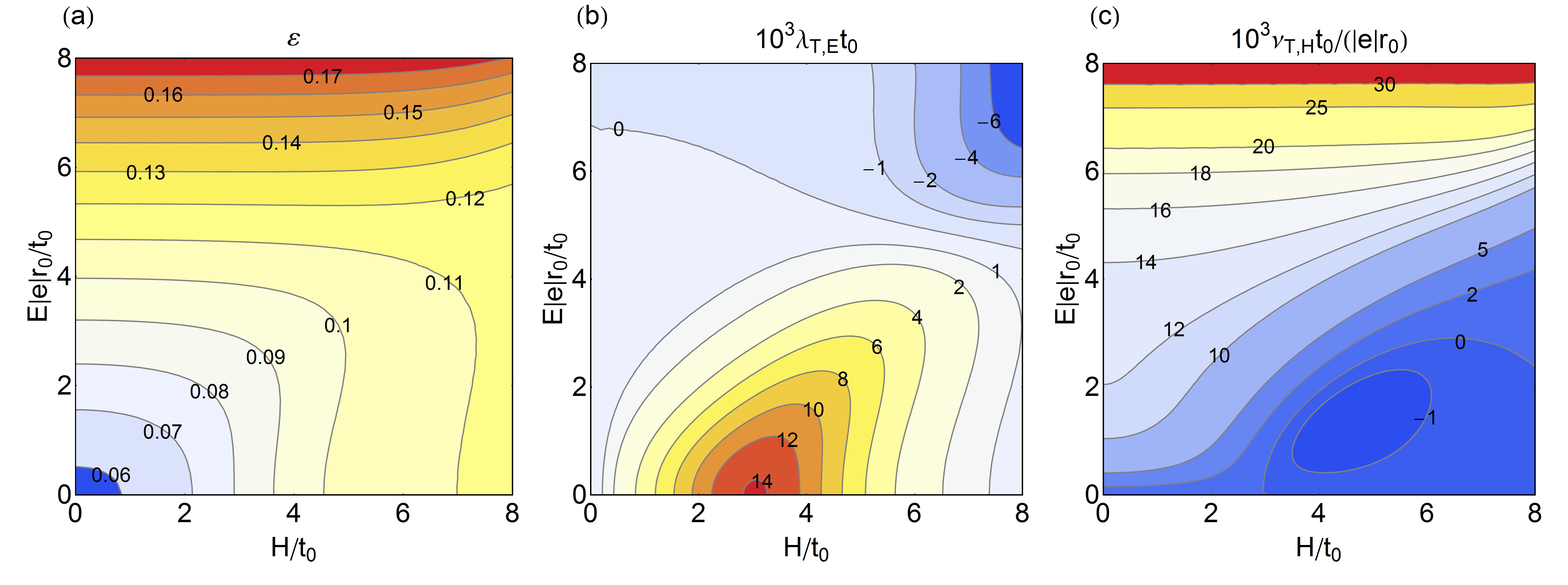
Figure 10: Contour plots of (a) relative deformation of dimer length; (b) normalized magnetostriction coefficient; (c) normalized electrostriction coefficient - as a function of normalized electric and magnetic field, for $U/t_{0}=2$ and $k_{\rm B}T/t_{0}=1.0$.

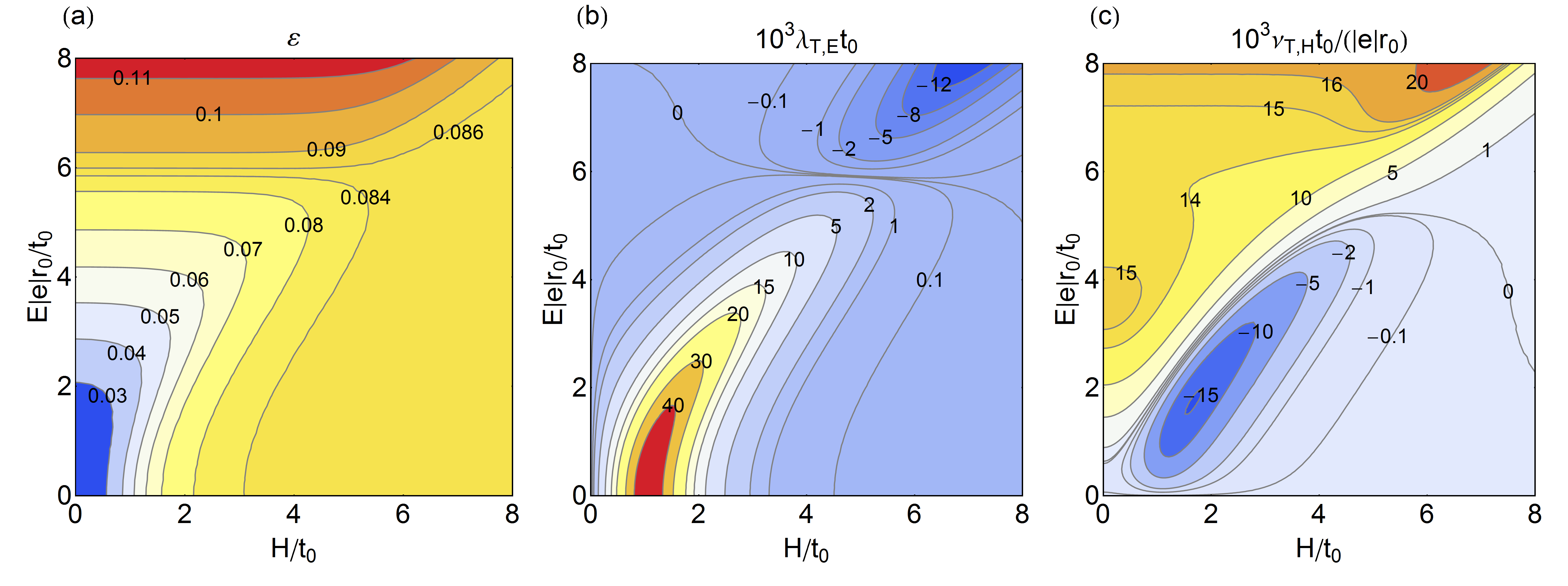
Figure 11: Contour plots of (a) relative deformation of dimer length; (b) normalized magnetostriction coefficient; (c) normalized electrostriction coefficient - as a function of normalized electric and magnetic field, for $U/t_{0}=5$ and $k_{\rm B}T/t_{0}=0.5$.

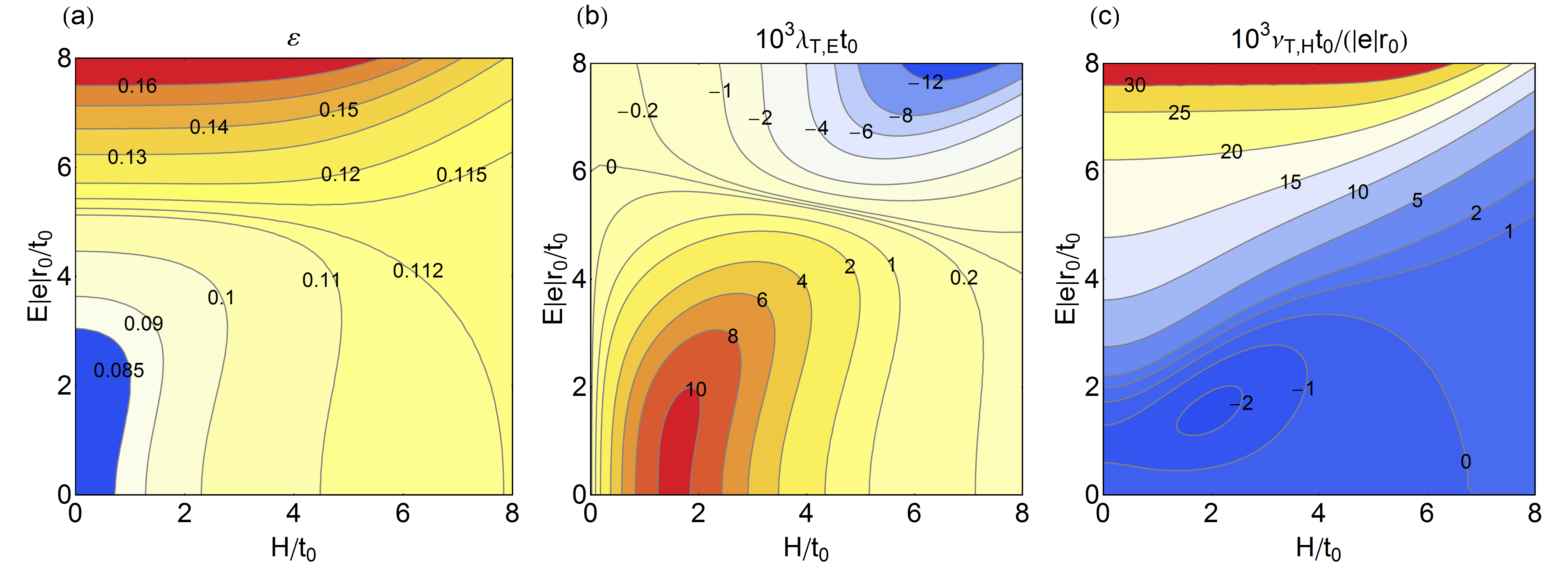
Figure 12: Contour plots of (a) relative deformation of dimer length; (b) normalized magnetostriction coefficient; (c) normalized electrostriction coefficient - as a function of normalized electric and magnetic field, for $U/t_{0}=5$ and $k_{\rm B}T/t_{0}=1.0$.

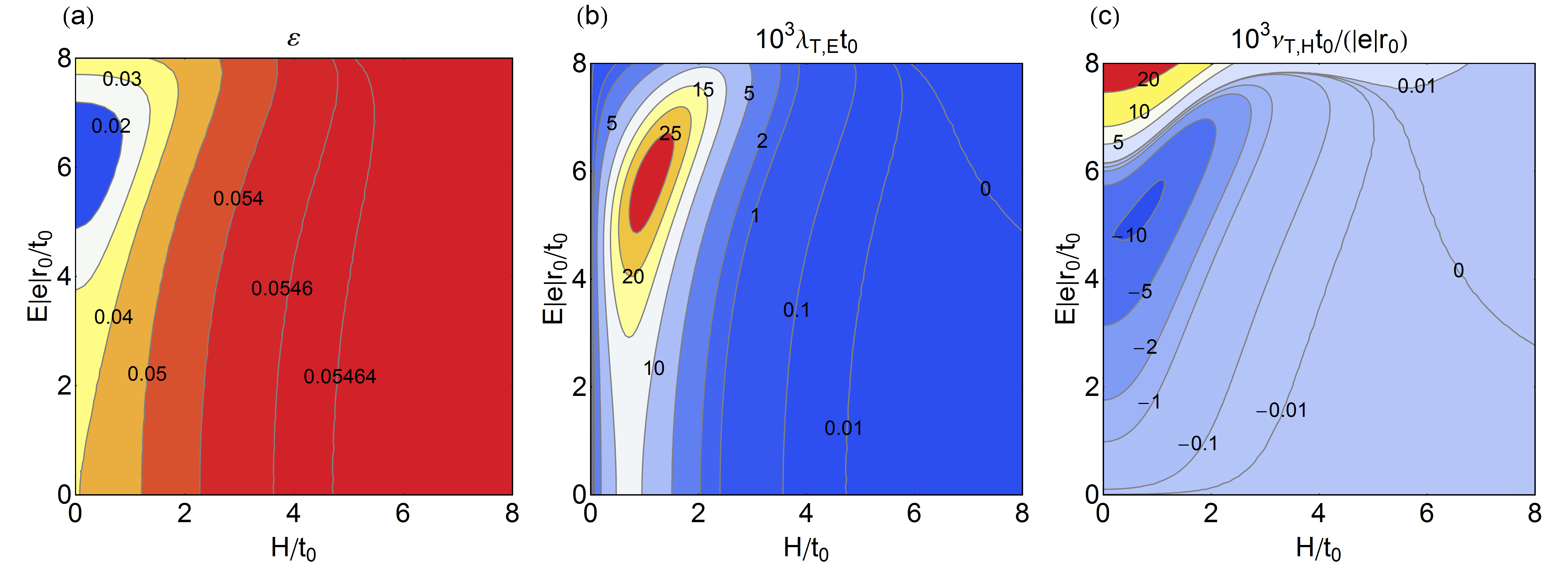
Figure 13: Contour plots of (a) relative deformation of dimer length; (b) normalized magnetostriction coefficient; (c) normalized electrostriction coefficient - as a function of normalized electric and magnetic field, for $U/t_{0}=10$ and $k_{\rm B}T/t_{0}=0.5$.

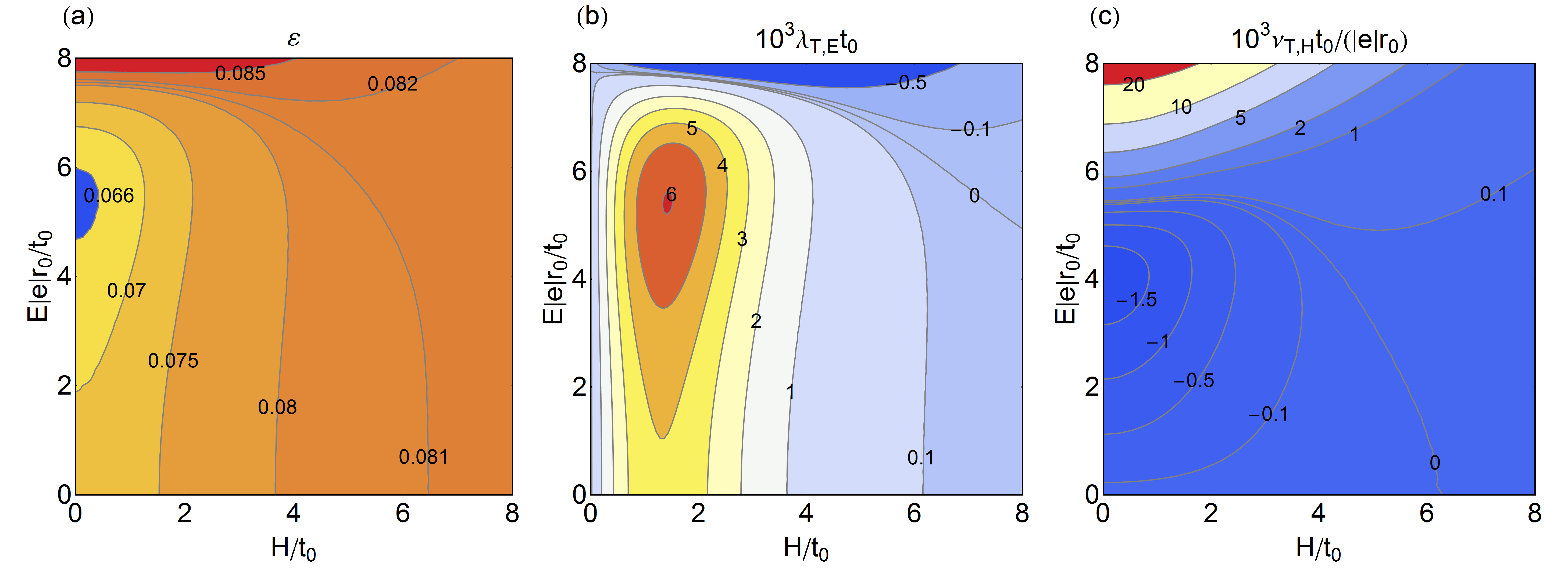
Figure 14: Contour plots of (a) relative deformation of dimer length; (b) normalized magnetostriction coefficient; (c) normalized electrostriction coefficient - as a function of normalized electric and magnetic field, for $U/t_{0}=10$ and $k_{\rm B}T/t_{0}=1.0$.

The next figures (Fig. 9-14) are prepared in form of contour graphs, presenting in the multiple charts the deformation (in parts a), magnetostriction coefficient (in parts b) and electrostriction coefficient (in parts c). The isolines of the dimensionless quantities, $\varepsilon$, $1000\times\lambda_{T,E}t_{0}$, and $1000\times\nu_{T,H}t_{0}/(|e|r_{0})$, are plotted as a function of the external fields, in the plane ($H/t_{0},\,E|e|r_{0}/t_{0}$). Two temperatures, which are far from the ground state: $k_{\rm B}T/t_{0}=0.5$ (for Fig. 9, 11, and 13), and $k_{\rm B}T/t_{0}=1.0$ (for Fig. 10, 12, and 14) are chosen. In order to illustrate the role of Coulombic on-site repulsion $U$, three values are selected: $U/t_{0}=2$ for LABEL:fig9,fig10, $U/t_{0}=5$ for LABEL:fig11,fig12, and $U/t_{0}=10$ for LABEL:fig13,fig14.

We see that both $T$ and $U$ play a significant role in the behaviour of the quantities presented in multiple contour plots. The shapes of the isolines, defining the areas with similar values of the presented quantities, change dynamically between different plots. In particular, analysing the deformation, it can be noted that areas with the smallest values of $\varepsilon$, denoted by blue shades and situated in the left parts of the charts, where rather small magnetic fields dominate, are shifted quite irregularly along the vertical (electric field) axis for different $T$ and $U$. At the same time, the areas with highest values of $\varepsilon$, denoted by red colour and other warm shades, are expanding as the temperature increases for each value of $U$. For instance, analysing the isolines for $\varepsilon$ $=$ 0.1 in Fig. 9(a)-12(a) for given $U$, we see that the areas with $\varepsilon\geq$0.1 are increasing when $T$ increases. On the other hand, all isolines in 14(a) correspond to larger values of $\varepsilon$ than isolines in 13(a). The red areas are situated at high electric fields when $U/t_{0}=2$ and $U/t_{0}=5$, however, when $U/t_{0}=10$, the area with large $\varepsilon$ extends over all values of the electric fields down to zero, provided the magnetic field is not very small. It should be stressed that deformation $\varepsilon$ is positive for all these cases. The increasing values of $\varepsilon$ when the temperature increases indicate that also the thermal expansion coefficient should be positive.

Regarding the magnetostriction, its value is mostly positive, however, some areas with the negative magnetostriction can be found, namely for high magnetic and electric fields. Interestingly, the area with negative magnetostriction expands with the increasing temperature. On the other hand, the dependency on $U$ is not monotonous: although the area with negative magnetostriction is larger for $U/t_{0}=5$ than for $U/t_{0}=2$, however, for $U/t_{0}=10$ this range becomes strongly reduced and is only visible at higher temperature ($k_{\rm B}T/t_{0}=1.0$). The area where the highest magnetostriction occurs lies in the range belonging to small electric fields, provided that $U/t_{0}=2$ or $U/t_{0}=5$, however, it is shifted towards large electric fields if $U/t_{0}=10$. The magnetic fields are moderate in all cases of high magnetostriction ranges, being from the range of ($2\lesssim H/t_{0}\lesssim 4$) for $U/t_{0}=2$, and ($0.5\lesssim H/t_{0}\lesssim 2$) for higher $U/t_{0}$. The increase in temperature results also in some expansion of the area with strong positive magnetostriction. It can also be noted that isolines corresponding to zero magnetostriction present an interesting behaviour, namely, the increase in electric field causes the decrease in the magnetic field along the isoline, so that the slope of the line as a function of $H$ is negative.

As far as the electrostriction coefficient is concerned, some areas with the negative values of this quantity are also observed in all the cases. For small values of $U$ these areas lie at low electric fields. In particular, for $U/t_{0}=2$, rather high magnetic fields ($H/t_{0}\gtrsim 3$) are involved, whereas for $U/t_{0}=5$ the corresponding magnetic fields are much lower. They may extend down even until $H/t_{0}=0$, as in the case of 12. On the other hand, for $U/t_{0}=10$ the area with negative electrostriction occurs for considerably higher electric fields, for instance, in the order of $E|e|r_{0}/t_{0}\approx 4$, whereas the magnetic fields are still very small. The increase in temperature, from $k_{\rm B}T/t_{0}=0.5$ to $k_{\rm B}T/t_{0}=1.0$, makes the area of negative electrostriction larger, but, at the same time, its amplitude decreases approximately by an order of magnitude. On the other hand, the areas corresponding to the highest positive electrostriction are mainly situated at very large electric fields. An exception is 9 where, for $U/t_{0}=2.0$ and $k_{\rm B}T/t_{0}=0.5$, the region of positive electrostriction coefficient extends down to very small electric fields.

In general, the isolines separating the areas of positive and negative electrostriction are more densely packed for $k_{\rm B}T/t_{0}=0.5$ than for $k_{\rm B}T/t_{0}=1.0$. The oblique arrangement of these lines at $k_{\rm B}T/t_{0}=0.5$ may lead to considerable dynamics of the electrostriction coefficient when crossing them horizontally by an increase in the magnetic field. The isolines corresponding to zero electrostriction effect can reveal either positive or negative slope as a function of the magnetic field $H$. The positive slope occurs, first of all, in the range of small magnetic fields, whereas for larger $H$ values the negative slopes are dominating (see, for instance LABEL:fig11,fig12 for $U/t_{0}=5$). This contrasts with the behaviour of the magnetostriction, where the slopes of the null magnetostriction coefficient line were always negative.

4 Summary and conclusion

In the paper the total grand potential has been constructed for the dimer system, in which the magnetic, elastic and thermal vibration energies play important roles. The similar attempts at the total Gibbs energy construction, i.e., consisting in summation of various energy contributions, have been undertaken, so far, for the bulk materials [61, 63, 64, 65, 66]. According to our knowledge, for the Hubbard dimer such method has not been presented previously.

It should be mentioned that also another approach to the problem can be proposed, namely, including the term representing electron–phonon interaction into the common Hamiltonian, and application of canonical transformation of Lang–Firsov type [68, 69, 70, 71, 72]. Then, the procedure is followed by using the 2nd order perturbation calculus, or, equivalently, by the Schrieffer–Wolff transformation [69], which leads to the renormalization of Hamiltonian parameters. Such a method is much more complicated and, in our opinion, is therefore less convenient for the complete studies of various thermodynamic properties. Moreover, the Lang–Firsov type transformation has been proposed for the Hamiltonians describing the coupling of electrons with the harmonic oscillators [70], whereas in our approach the anharmonic vibrations are taken into account via Grüneisen parameter $\Gamma$. It is known that the anharmonicity plays an important role, for instance, in the studies of thermal expansion effect.

As a result of the present approach, the EOS (Eq. 27) has been derived for the system in question. This equation yields stable solutions for the interatomic distance deformation, $\varepsilon$, corresponding to the thermodynamic equilibrium state obtained at arbitrary temperature $T$ and the external fields $H$ and $E$. Investigation of this deformation leads to the determination of its derivative quantities such as the thermal expansion or magneto- and electrostriction coefficients.

It has been shown in the paper that for the half-filling conditions ($x=1$) and for the elastic interactions included, the chemical potential $\mu$ is not a constant but it depends, via the quantity $\varepsilon$, on the temperature and external fields (Fig. 1-3). For $x=1$ the analytic formula describing $\mu$ has been presented (Eq. 21). It should be stressed that the method used here can be equally well applied to arbitrary average concentration of the electrons, i.e., when $0\leq\;x\leq 2$.

In the low-temperature region, where the quantum phase transitions are induced by the external fields, the discontinuous changes of deformation $\varepsilon$ have been found at the phase transition points. These discontinuous changes are also accompanied by discontinuities of such quantities as the magnetostriction and electrostriction coefficients (Fig. 4-7). It is known that with an increase in temperature the quantum phase transitions become diffused, so then, the most spectacular effects of discontinuity occur at $T\to 0$.

For the asymmetric interatomic potential, an increase in temperature results in the linear expansivity effect. In our opinion, an interesting finding concerns the broad maxima of the thermal expansion coefficient, found at some temperatures and illustrated in 8. It has been shown that the positions of maxmima are strongly dependent on the values of Hubbard $U$ parameter.

In the high-temperature region, where the discontinuities of thermodynamic quantities do not occur, the contour charts yield a comprehensive description of the interatomic distance deformation and its changes vs. external fields. The contour charts (Fig. 9-14) have been used to illustrate simultaneously $\varepsilon$, as well as the magnetostriction and electrostriction coefficients vs. $H$ and $E$, for some selection of temperatures $T$ and parameters $U$. In particular, a distinctive result is an identification of the ($H,E$)-regions where the negative values of these coefficients do appear. It has been found that both temperature $T$ and $U$-parameter have important influence on the localization and area of these regions, as well as on the values of $\varepsilon$, $\lambda_{T,E}$, and $\nu_{T,H}$ themselves.

To summarize, by taking into consideration the elastic interactions and thermal vibrations, a new, more complete thermodynamic description of the Hubbard dimer has been achieved. It should be stressed that diagonalization of the Hubbard Hamiltonian has been performed exactly by means of the analytical methods [41]. It can be expected that selection of other interatomic potentials would change our results quantitatively; however, the case which we consider in the present paper captures the essence of the phenomena emerging due to coupling between purely electronic and elastic properties.

It should also be pointed out that having constructed the total grand potential, all thermodynamic and statistical properties of the system can be studied. For instance, this allows the self-consistent calculation of the magnetization, electric polarization, magnetic correlation functions, occupation correlations, susceptibility (both magnetic and electric one), entropy and specific heat, in the presence of the elastic interactions.

Figure 1: The normalized deviation of the chemical potential from the value of $U/2$ expected for pure Hubbard model as a function of the normalized temperature, for a few selected values of normalized on-site Hubbard energy $U/t_{0}$ in the absence of the external fields.

Figure 2: The normalized deviation of the chemical potential from the value of $U/2$ expected for pure Hubbard model as a function of the normalized magnetic field, for a few selected values of normalized on-site Hubbard energy $U/t_{0}$, in the absence of the electric field and for moderate temperature $k_{\rm B}T/t_{0}=0.5$.

Figure 3: The normalized deviation of the chemical potential from the value of $U/2$ expected for pure Hubbard model as a function of the normalized electric field, for a few selected values of normalized on-site Hubbard energy $U/t_{0}$, in the absence of the magnetic field and for moderate temperature $k_{\rm B}T/t_{0}=0.5$.

Figure 4: The relative deformation of dimer length as a function of the normalized magnetic field, for a few selected values of normalized on-site Hubbard energy $U/t_{0}$, in the absence of the electric field and for low temperature $k_{\rm B}T/t_{0}=10^{-3}$.

Figure 5: The normalized electrostriction coefficient as a function of the normalized magnetic field, for a few selected values of normalized on-site Hubbard energy $U/t_{0}$, for the normalized electric field of $E|e|d/t_{0}=0.5$ and for low temperature $k_{\rm B}T/t_{0}=10^{-3}$.

Figure 6: The relative deformation of dimer length as a function of the normalized electric field, for a few selected values of normalized on-site Hubbard energy $U/t_{0}$, for the normalized magnetic field $H/t_{0}=4.8$ and for low temperature $k_{\rm B}T/t_{0}=10^{-3}$.

Figure 7: The normalized magnetostriction coefficient as a function of the normalized electric field, for a few selected values of normalized on-site Hubbard energy $U/t_{0}$, for the normalized magnetic field of $H/t_{0}=4.8$ and for two normalized temperatures: $k_{\rm B}T/t_{0}=0.05$ and $0.1$.

Figure 8: The normalized thermal expansion coefficient as a function of the normalized temperature, for a few selected values of normalized on-site Hubbard energy $U/t_{0}$, in the absence of the external fields.

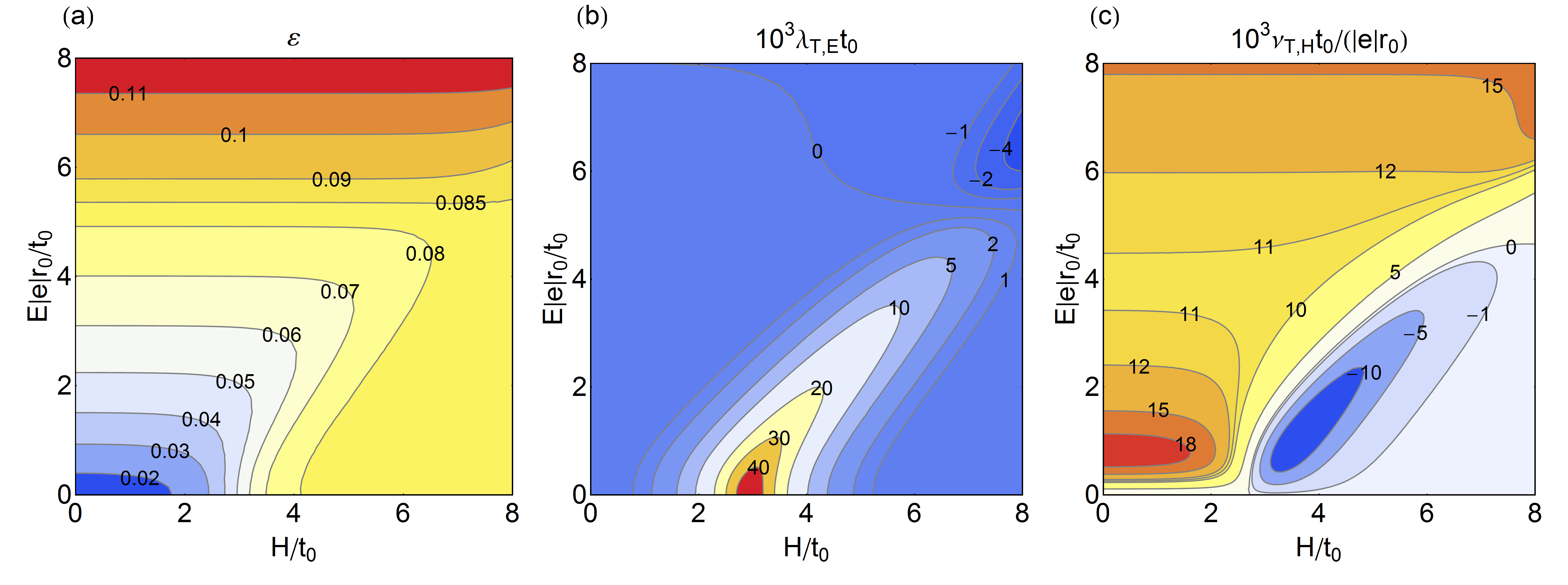
Figure 9: Contour plots of (a) relative deformation of dimer length; (b) normalized magnetostriction coefficient; (c) normalized electrostriction coefficient - as a function of normalized electric and magnetic field, for $U/t_{0}=2$ and $k_{\rm B}T/t_{0}=0.5$.

References

- [1] P. W. Anderson, New Approach to the Theory of Superexchange Interactions, Phys. Rev. 115 (1) (1959) 2–13. doi:10.1103/PhysRev.115.2.
- [2] J. Hubbard, Electron Correlations in Narrow Energy Bands, Proceedings of the Royal Society of London A: Mathematical, Physical and Engineering Sciences 276 (1365) (1963) 238–257. doi:10.1098/rspa.1963.0204.
- [3] M. C. Gutzwiller, Effect of Correlation on the Ferromagnetism of Transition Metals, Phys. Rev. Lett. 10 (5) (1963) 159–162. doi:10.1103/PhysRevLett.10.159.
- [4] J. Kanamori, Electron Correlation and Ferromagnetism of Transition Metals, Progress of Theoretical Physics 30 (3) (1963) 275–289. doi:10.1143/PTP.30.275.
- [5] W. Nolting, A. Ramakanth, Quantum Theory of Magnetism, Springer-Verlag, Berlin, 2009.
- [6] K. Yosida, Theory of Magnetism, Springer-Verlag, Berlin, 1998.
- [7] H. Tasaki, The Hubbard model - an introduction and selected rigorous results, Journal of Physics: Condensed Matter 10 (20) (1998) 4353. doi:10.1088/0953-8984/10/20/004.
- [8] A. Mielke, The Hubbard Model and its Properties, in: E. Pavarini, E. Koch, P. Coleman (Eds.), Many-Body Physics: From Kondo to Hubbard. Modeling and Simulation, Vol. 5, Verlag des Forschungszentrum Jülich, Jülich, 2015. hdl.handle.net/2128/9255.
- [9] B. S. Shastry, Exact Integrability of the One-Dimensional Hubbard Model, Phys. Rev. Lett. 56 (23) (1986) 2453–2455. doi:10.1103/PhysRevLett.56.2453.
- [10] J. E. Hirsch, S. Tang, Antiferromagnetism in the Two-Dimensional Hubbard Model, Phys. Rev. Lett. 62 (5) (1989) 591–594. doi:10.1103/PhysRevLett.62.591.
- [11] S. Fuchs, E. Gull, L. Pollet, E. Burovski, E. Kozik, T. Pruschke, M. Troyer, Thermodynamics of the 3D Hubbard Model on Approaching the Néel Transition, Phys. Rev. Lett. 106 (3) (2011) 030401. doi:10.1103/PhysRevLett.106.030401.
- [12] Y. Ohta, K. Tsutsui, W. Koshibae, S. Maekawa, Exact-diagonalization study of the Hubbard model with nearest-neighbor repulsion, Physical Review B 50 (18) (1994) 13594–13602. doi:10.1103/PhysRevB.50.13594.
- [13] M. A. Ojeda-López, J. Dorantes-Dávila, G. M. Pastor, Magnetic properties of Hubbard clusters: Noncollinear spins in N-atom clusters, Journal of Applied Physics 81 (8) (1997) 4170–4172. doi:10.1063/1.365128.
- [14] C. Noce, M. Cuoco, A. Romano, Thermodynamical properties of the Hubbard model on finite-size clusters, Physica C: Superconductivity 282-287 (1997) 1705–1706. doi:10.1016/S0921-4534(97)00972-6.
- [15] M. A. Ojeda, J. Dorantes-Dávila, G. M. Pastor, Noncollinear cluster magnetism in the framework of the Hubbard model, Physical Review B 60 (8) (1999) 6121–6130. doi:10.1103/PhysRevB.60.6121.
- [16] F. Becca, A. Parola, S. Sorella, Ground-state properties of the Hubbard model by Lanczos diagonalizations, Physical Review B 61 (24) (2000) R16287–R16290. doi:10.1103/PhysRevB.61.R16287.
- [17] J. L. Ricardo-Chávez, F. Lopez-Urías, G. M. Pastor, Thermal Properties of Magnetic Clusters, in: J. L. Morán-López (Ed.), Physics of Low Dimensional Systems, Kluwer Academic/Plenum Publishers, New York, 2001, pp. 23–32. doi:10.1007/0-306-47111-6_3.
- [18] Y. Hancock, A. E. Smith, Application of the Hubbard model with external field to quasi-zero dimensional, inhomogeneous systems, Physics Letters A 300 (4) (2002) 491–499. doi:10.1016/S0375-9601(02)00854-X.
- [19] Y. Hancock, Quasi-zero-dimensional quantum spin-switching system, Physical Review B 71 (22) (2005) 224428. doi:10.1103/PhysRevB.71.224428.
- [20] R. Schumann, Analytical solution of extended Hubbard models on three- and four-site clusters, Physica C: Superconductivity 460-462 (2007) 1015–1017. doi:10.1016/j.physc.2007.03.203.
- [21] R. Schumann, Rigorous solution of a Hubbard model extended by nearest-neighbour Coulomb and exchange interaction on a triangle and tetrahedron, Annalen der Physik 17 (4) (2008) 221–259. doi:10.1002/andp.200710281.
- [22] S. X. Yang, H. Fotso, J. Liu, T. A. Maier, K. Tomko, E. F. D’Azevedo, R. T. Scalettar, T. Pruschke, M. Jarrell, Parquet approximation for the 4x4 Hubbard cluster, Physical Review E 80 (4) (2009) 046706. doi:10.1103/PhysRevE.80.046706.
- [23] R. Schumann, D. Zwicker, The Hubbard model extended by nearest-neighbor Coulomb and exchange interaction on a cubic cluster - rigorous and exact results, Annalen der Physik 522 (6) (2010) 419–439. doi:10.1002/andp.201010452.
- [24] H. Feldner, Z. Y. Meng, A. Honecker, D. Cabra, S. Wessel, F. F. Assaad, Magnetism of finite graphene samples: Mean-field theory compared with exact diagonalization and quantum Monte Carlo simulations, Phys. Rev. B 81 (11) (2010) 115416. doi:10.1103/PhysRevB.81.115416.
- [25] M. Y. Ovchinnikova, Spin Structures of the Hubbard Clusters and the Pseudogap, Journal of Superconductivity and Novel Magnetism 26 (9) (2013) 2845–2846. doi:10.1007/s10948-013-2218-0.
- [26] Y. Hancock, A family of spin-switching, inhomogeneous Hubbard chains, Physica E: Low-dimensional Systems and Nanostructures 56 (2014) 141–150. doi:10.1016/j.physe.2013.08.021.
- [27] T. X. R. Souza, C. A. Macedo, Ferromagnetic Ground States in Face-Centered Cubic Hubbard Clusters, PLOS ONE 11 (9) (2016) e0161549. doi:10.1371/journal.pone.0161549.
- [28] K. Szałowski, T. Balcerzak, M. Jaščur, A. Bobák, M. Žukovič, Exact Diagonalization Study of an Extended Hubbard Model for a Cubic Cluster at Quarter Filling, Acta Physica Polonica A 131 (4) (2017) 1012–1014. doi:10.12693/APhysPolA.131.1012.
- [29] K. Szałowski, T. Balcerzak, Electrocaloric effect in cubic Hubbard nanoclusters, Scientific Reports 8 (1) (2018) 5116. doi:10.1038/s41598-018-23443-x.
- [30] B. Alvarez-Fernández, J. A. Blanco, The Hubbard model for the hydrogen molecule, European Journal of Physics 23 (1) (2002) 11. doi:10.1088/0143-0807/23/1/302.
- [31] A. B. Harris, R. V. Lange, Single-Particle Excitations in Narrow Energy Bands, Phys. Rev. 157 (2) (1967) 295–314. doi:10.1103/PhysRev.157.295.
- [32] R. Wortis, M. P. Kennett, Local integrals of motion in the two-site Anderson-Hubbard model, Journal of Physics: Condensed Matter 29 (40) (2017) 405602. doi:10.1088/1361-648X/aa818e.
- [33] Y.-C. Cheng, K.-C. Liu, Thermodynamic Properties of a Two-Site Hubbard Hamiltonian: Half-Filled-Band Case, Chinese Journal of Physics 14 (3) (1976) 325–328.
- [34] S. Longhi, G. Della Valle, V. Foglietti, Classical realization of two-site Fermi-Hubbard systems, Phys. Rev. B 84 (3) (2011) 033102. doi:10.1103/PhysRevB.84.033102.
- [35] R. C. Juliano, A. S. de Arruda, L. Craco, Coexistence and competition of on-site and intersite Coulomb interactions in Mott-molecular-dimers, Solid State Communications 227 (2016) 51 – 55. doi:http://dx.doi.org/10.1016/j.ssc.2015.11.021.
- [36] M. E. Kozlov, V. A. Ivanov, K. Yakushi, Development of a two-site Hubbard model for analysis of the electron-molecular vibration coupling in organic charge-transfer salts, Physics Letters A 214 (3) (1996) 167 – 174. doi:http://dx.doi.org/10.1016/0375-9601(96)00113-2.
- [37] A. V. Silant’ev, A Dimer in the Extended Hubbard Model, Russian Physics Journal 57 (11) (2015) 1491–1502. doi:10.1007/s11182-015-0406-z.
- [38] H. Hasegawa, Nonextensive thermodynamics of the two-site Hubbard model, Physica A: Statistical Mechanics and its Applications 351 (2-4) (2005) 273 – 293. doi:http://dx.doi.org/10.1016/j.physa.2005.01.025.
- [39] H. Hasegawa, Thermal entanglement of Hubbard dimers in the nonextensive statistics, Physica A: Statistical Mechanics and its Applications 390 (8) (2011) 1486 – 1503. doi:http://dx.doi.org/10.1016/j.physa.2010.12.033.
- [40] J. Spałek, A. M. Oleś, K. A. Chao, Thermodynamic properties of a two-site Hubbard model with orbital degeneracy, Physica A: Statistical Mechanics and its Applications 97 (3) (1979) 552 – 564. doi:http://dx.doi.org/10.1016/0378-4371(79)90095-5.
- [41] T. Balcerzak, K. Szałowski, Hubbard pair cluster in the external fields. Studies of the chemical potential, Physica A: Statistical Mechanics and its Applications 468 (2017) 252–266. doi:10.1016/j.physa.2016.11.004.
- [42] T. Balcerzak, K. Szałowski, Hubbard pair cluster in the external fields. Studies of the magnetic properties, Physica A: Statistical Mechanics and its Applications 499 (2018) 395–406. doi:10.1016/j.physa.2018.02.017.
- [43] T. Balcerzak, K. Szałowski, Hubbard pair cluster in the external fields. Studies of the polarization and susceptibility, Physica A: Statistical Mechanics and its Applications 512 (2018) 1069–1084. doi:10.1016/j.physa.2018.08.152.
- [44] C. A. Ullrich, Density-functional theory for systems with noncollinear spin: Orbital-dependent exchange-correlation functionals and their application to the Hubbard dimer, Physical Review B 98 (3) (2018) 035140. doi:10.1103/PhysRevB.98.035140.
- [45] F. Sagredo, K. Burke, Accurate double excitations from ensemble density functional calculations, The Journal of Chemical Physics 149 (13) (2018) 134103. doi:10.1063/1.5043411.
- [46] D. J. Carrascal, J. Ferrer, J. C. Smith, K. Burke, The Hubbard dimer: A density functional case study of a many-body problem, Journal of Physics: Condensed Matter 27 (39) (2015) 393001. doi:10.1088/0953-8984/27/39/393001.
- [47] J. I. Fuks, N. T. Maitra, Charge transfer in time-dependent density-functional theory: Insights from the asymmetric Hubbard dimer, Physical Review A 89 (6) (2014) 062502. doi:10.1103/PhysRevA.89.062502.
- [48] E. Kamil, R. Schade, T. Pruschke, P. E. Blöchl, Reduced density-matrix functionals applied to the Hubbard dimer, Physical Review B 93 (8) (2016) 085141. doi:10.1103/PhysRevB.93.085141.
- [49] S. Balasubramanian, J. K. Freericks, Exact Time Evolution of the Asymmetric Hubbard Dimer, Journal of Superconductivity and Novel Magnetism 30 (1) (2017) 97–102. doi:10.1007/s10948-016-3811-9.
- [50] J. Čisárová, J. Strečka, Exact solution of a coupled spin-electron linear chain composed of localized Ising spins and mobile electrons, Physics Letters A 378 (38-39) (2014) 2801 – 2807. doi:http://dx.doi.org/10.1016/j.physleta.2014.07.049.
- [51] M. Nalbandyan, H. Lazaryan, O. Rojas, S. Martins de Souza, N. Ananikian, Magnetic, Thermal, and Entanglement Properties of a Distorted Ising-Hubbard Diamond Chain, Journal of the Physical Society of Japan 83 (7) (2014) 074001. doi:10.7566/JPSJ.83.074001.
- [52] L. Gálisová, J. Strečka, Magnetic Grüneisen parameter and magnetocaloric properties of a coupled spin–electron double-tetrahedral chain, Physics Letters A 379 (39) (2015) 2474–2478. doi:10.1016/j.physleta.2015.07.007.
- [53] L. Gálisová, J. Strečka, Vigorous thermal excitations in a double-tetrahedral chain of localized Ising spins and mobile electrons mimic a temperature-driven first-order phase transition, Physical Review E 91 (2) (2015) 022134. doi:10.1103/PhysRevE.91.022134.
- [54] H. Čenčariková, J. Strečka, M. L. Lyra, Reentrant phase transitions of a coupled spin-electron model on doubly decorated planar lattices with two or three consecutive critical points, Journal of Magnetism and Magnetic Materials 401 (2016) 1106 – 1122. doi:http://dx.doi.org/10.1016/j.jmmm.2015.11.018.
- [55] N. Ananikian, Č. Burdík, L. Ananikyan, H. Poghosyan, Magnetization Plateaus and Thermal Entanglement of Spin Systems, Journal of Physics: Conference Series 804 (2017) 012002. doi:10.1088/1742-6596/804/1/012002.
- [56] H. Čenčariková, J. Strečka, Enhanced magnetoelectric effect of the exactly solved spin-electron model on a doubly decorated square lattice in the vicinity of a continuous phase transition, Physical Review E 98 (6) (2018) 062129. doi:10.1103/PhysRevE.98.062129.
- [57] H. S. Sousa, M. S. S. Pereira, I. N. de Oliveira, J. Strečka, M. L. Lyra, Phase diagram and re-entrant fermionic entanglement in a hybrid Ising-Hubbard ladder, Physical Review E 97 (5) (2018) 052115. doi:10.1103/PhysRevE.97.052115.
- [58] P. M. Morse, Diatomic Molecules According to the Wave Mechanics. II. Vibrational Levels, Physical Review 34 (1) (1929) 57–64. doi:10.1103/PhysRev.34.57.
- [59] L. A. Girifalco, V. G. Weizer, Application of the Morse Potential Function to Cubic Metals, Physical Review 114 (3) (1959) 687–690. doi:10.1103/PhysRev.114.687.
- [60] E. Grüneisen, Theorie des festen Zustandes einatomiger Elemente, Annalen der Physik 344 (12) (1912) 257–306. doi:10.1002/andp.19123441202.
- [61] T. Balcerzak, K. Szałowski, M. Jaščur, A simple thermodynamic description of the combined Einstein and elastic models, Journal of Physics: Condensed Matter 22 (42) (2010) 425401. doi:10.1088/0953-8984/22/42/425401.
- [62] A. M. Krivtsov, V. A. Kuz’kin, Derivation of equations of state for ideal crystals of simple structure, Mechanics of Solids 46 (3) (2011) 387. doi:10.3103/S002565441103006X.
- [63] T. Balcerzak, K. Szałowski, M. Jaščur, A self-consistent thermodynamic model of metallic systems. Application for the description of gold, Journal of Applied Physics 116 (4) (2014) 043508. doi:10.1063/1.4891251.
- [64] T. Balcerzak, K. Szałowski, M. Jaščur, Self-consistent model of a solid for the description of lattice and magnetic properties, Journal of Magnetism and Magnetic Materials 426 (2017) 310–319. doi:10.1016/j.jmmm.2016.11.107.
- [65] T. Balcerzak, K. Szałowski, M. Jaščur, Thermodynamic model of a solid with RKKY interaction and magnetoelastic coupling, Journal of Magnetism and Magnetic Materials 452 (2018) 360–372. doi:10.1016/j.jmmm.2017.12.088.
- [66] K. Szałowski, T. Balcerzak, M. Jaščur, Thermodynamics of a model solid with magnetoelastic coupling, Journal of Magnetism and Magnetic Materials 445 (2018) 110–118. doi:10.1016/j.jmmm.2017.08.073.
- [67] L. Goodwin, A. J. Skinner, D. G. Pettifor, Generating Transferable Tight-Binding Parameters: Application to Silicon, Europhys. Letters 9 (1989) 701–706. doi:10.1209/0295-5075/9/7/0151.
- [68] I. G. Lang, Yu. A. Firsov, Kinetic Theory of Semiconductors with Low Mobility, Zh. Eksp. Teor. Fiz. 43 (1962) 1843 (Sov. Phys. JETP 16 (1963) 1301). http://www.jetp.ac.ru/cgi-bin/dn/e_016_05_1301.pdf.
- [69] W. Stephan, M. Capone, M. Grilli, C. Castellani, Influence of electron-phonon interaction on superexchange, Phys. Lett. A 227 (1997) 120–126. doi:0.1016/S0375-9601(96)00950-4.
- [70] V. M. Stojanović, P. A. Bobbert, M. A. J. Michels, Nonlocal electron-phonon coupling: Consequences for the nature of polaron states, Phys. Rev. B 69 (2004) 144302. doi:10.1103/PhysRevB.69.144302.
- [71] J. Koch, Quantum transport through single-molecule devices. PhD thesis, Freie Universität Berlin (2006). https://refubium.fu-berlin.de/handle/fub188/13330.
- [72] M. Hohenadler, W. von der Linden, Lang-Firsov Approaches to Polaron Physics: From Variational Methods to Unbiased Quantum Monte Carlo Simulations, In: Alexandrov A.S. (eds) Polarons in Advanced Materials. Springer Series in Materials Science, vol 103. Springer, Dordrecht (2007). doi:10.1007/978-1-4020-6348-0_11.