Lensing anomaly and oscillations in the primordial power spectrum

Abstract

The latest analysis of the cosmic microwave background by the Planck team finds more smoothing of the acoustic peaks in the temperature power spectrum than predicted by $\Lambda$CDM. Here we investigate whether this additional smoothing can be mimicked by an oscillatory feature, generated during inflation, that is similar to the acoustic peaks but out of phase. We consider oscillations generated by oscillating modulations of the background—e.g., due to heavy fields or modulated potentials—and by sharp features. We show that it is difficult to induce oscillations that are linear (or almost linear) in $k$ by oscillatory modulations of the background. We find, however, that a sharp bumpy feature in the sound speed of perturbations is able to produce the desired oscillations. The scenario can be tested by combining CMB and BAO data.

I Introduction

As cosmic microwave background (CMB) photons travel towards us, their trajectories are deflected by the gravitational potentials generated by the matter distribution. This weak lensing of the CMB has an impact on the CMB temperature power spectrum Seljak (1996); Lewis and Challinor (2006). The lensing magnifies the angular size of the primordial fluctuations in some places on the sky and de-magnifies others. The observed peak structure in the temperature power spectrum, when measured over the entire sky, are therefore blurred Hanson et al. (2010): the acoustic peaks are reduced slightly, and the troughs between them filled in.

Interestingly, when the theoretical prediction for this smoothing is compared with the Planck data, it is found that the lensing smoothing is larger than expected by roughly $10\%$ Aghanim et al. (2018). The so-called $A_{L}$ anomaly is persistent and recently slightly more statistically significant, with a value $A_{L}=1.149\pm 0.072$ ($68\%$ confidence), that constitutes a $2\sigma$ tension with $\Lambda$CDM cosmology Aghanim et al. (2018). Moreover, the residuals between the signal and the theoretical prediction yield an oscillatory pattern whose frequency is roughly linear in the multipole number $\ell$ and similar in shape to the acoustic peaks.

If the tension persists with higher statistical significance, it might be explained by some new physics that mimicks the smoothing effect of lensing. One possibility discussed by the Planck collaboration Aghanim et al. (2018) is that there might be a component of cold dark matter isocurvature (CDI) perturbation with a blue tilt. Since the acoustic peaks of the CDI will have the opposite phase, this will effectively smooth out the photon acoustic peaks. A similar mechanism was also studied in Refs. Muñoz et al. (2016); Smith et al. (2017) where the isocurvature perturbations of dark matter and baryons compensate each other. However, these models are tightly constraint by their effects on the trispectrum Smith et al. (2017). Another possibility is that there are oscillations in the primordial power spectrum which have the same frequency but opposite phase with the acoustic peaks Aghanim et al. (2018). However, in an analysis where the oscillatory feature in the power spectrum has a $k$ independent amplitude and a frequency linear in $k$, no correlation between the amplitude of the oscillations and $A_{L}$ is found Akrami et al. (2018). Moreover, one reaches similar conclusions when reconstructing the power spectrum from raw data Hazra et al. (2014a, 2019). In particular, it was already pointed out in Ref. Hazra et al. (2014a) that there is a degeneracy between the effects of lensing and oscillating features in the primordial power spectrum. On the theoretical side, though, it is not clear whether physical models that might induce wiggles in the primordial power spectrum are required to do so with a scale-independent amplitude, nor with a precisely linear dependence on $k$. Previous fits to the residuals of the temperature power spectrum were pursued in Refs. Achucarro et al. (2014); Chen and Namjoo (2014); Hazra et al. (2014b, 2016, 2018) but a mimicking of the lensing effect from an inflationary model was not studied. Note that the reconstruction of the primordial power spectrum taking into account lensing also yields an oscillating feature Hazra et al. (2019). However, it is not clear what kind of inflationary model would give rise to such specific wiggle Hazra et al. (2019).

Here we explore inflationary models that might give rise to oscillatory features in the primordial power spectrum that might account for the $A_{L}$ anomaly. Oscillatory features generated during inflation usually have an oscillation frequency which has a logarithmic or linear dependence on $k$ (see Ref. Chluba et al. (2015) for a review). On one hand, the logarithmic dependence could be either because there is an oscillating modulation in the Lagrangian that depends linearly on the inflaton which is slowly rolling Pahud et al. (2009); Flauger et al. (2010) or because an extra massive field is oscillating around its minimum in which case it oscillates with a constant frequency and linearly in the cosmic time Chen (2012); Chen et al. (2015, 2016a). Also, successive turns in the multi-field inflationary trajectory yield a logarithmic dependence in $k$ Gao et al. (2013). On the other hand, a frequency linear in $k$ is typical from sharp transitions, e.g. steps in the potential or sudden turns in the field space, with a damped amplitude depending on the sharpness of the transition Starobinsky (1992); Kamionkowski and Liddle (2000); Gong and Stewart (2001); Stewart (2002); Adams et al. (2001); Kaloper and Kaplinghat (2003); Choe et al. (2004); Dvorkin and Hu (2010); Achucarro et al. (2011a); Adshead et al. (2012); Shiu and Xu (2011); Cespedes et al. (2012); Gao et al. (2013); Bartolo et al. (2013); Achucarro et al. (2014). Note that sharp transitions can be understood in terms of Bogoliubov transformations Kaloper and Kaplinghat (2003), since the negative frequency mode has been excited by the turn or step. It is also interesting to note that both logarithmic and linear $k$ dependences of the frequency may be related to a trans-planckian modulation Easther et al. (2005). There is another interesting case where the frequency goes as a power-law of $k$ Huang and Pi (2018); Domènech et al. (2019); this may occur, e.g., when there is a background oscillation with a time dependent frequency. See Refs. Chen (2012); Chen et al. (2018) for a power-law dependence in $k$ in alternatives scenarios to inflation.

This paper is organized as follows. In Sec. II we review the $A_{L}$ anomaly and the requirement for the oscillatory patterns in the power spectrum to mimick the lensing smoothing. In Sec. III, we study which features could potentially yield such oscillatory patterns and we conclude in Sec. IV. We discuss possible models in App. A and present details of the calculations in Apps. B and C.

II $A_{L}\,$ anomaly

The effect of weak lensing onto the CMB power spectrum is to smooth out the acoustic peaks by blurring the acoustic-peak structure in $\ell$ space (see Fig. 1). Using the modelled unlensed CMB power spectrum and the lensing potential, one can estimate the magnitude of the smoothing effect of lensing $A_{L}$ Lewis and Challinor (2006); Calabrese et al. (2008). However, if nothing more than a power-law inflationary spectrum of adiabatic perturbations and $\Lambda$CDM are assumed, then the observed power spectrum has been lensed $10\%$ more than expected Aghanim et al. (2018).

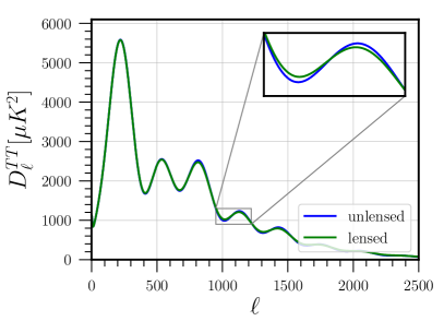
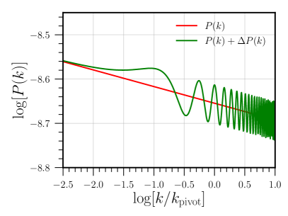
Figure 1: On the left, CMB temperature power spectrum. We respectively show the unlensed and lensed power spectrum in blue and green. See how the acoustic peaks are smoothed out. On the right, the oscillatory feature linear in $k$ in the primordial power spectrum vs the usual power-law spectrum.

This tension could conceivably by explained by an oscillatory modulation of the inflationary power spectrum which is out of phase with the acoustic peaks. To illustrate this, we introduce the following fitting to the inflationary power spectrum Chen (2012); Huang and Pi (2018); Domènech et al. (2019); Aghanim et al. (2018):

$$\frac{\Delta P_{\cal R}}{P_{{\cal R},0}}=A\left(\frac{k}{k_{*}}\right)^{n_{A}}\sin\left[\omega\left(\frac{k}{k_{*}}\right)^{n_{o}}+\varphi\right]$$ (1)

where the constants $A$, $k_{*}$, $\omega$, $\varphi$, $n_{A}$ and $n_{o}$ respectively are the amplitude, the pivot scale, the frequency, the phase and the power indexes of the $k$ in amplitude and frequency of the oscillation. These constants are ultimately related to parameters of a theoretical model. For example, the fitting form Eq. (1) appears in sudden transitions Starobinsky (1992); Kamionkowski and Liddle (2000); Gong and Stewart (2001); Stewart (2002); Adams et al. (2001); Choe et al. (2004); Dvorkin and Hu (2010); Achucarro et al. (2011a); Adshead et al. (2012); Shiu and Xu (2011); Cespedes et al. (2012); Gao et al. (2013); Bartolo et al. (2013); Achucarro et al. (2014), oscillating heavy fields Chen (2012); Huang and Pi (2018); Domènech et al. (2019) and trans-planckian modulations Easther et al. (2005) during inflation. Now, we translate it to the multipole number for a rough comparison as

$$\frac{\Delta C_{\ell}}{C_{{\ell},0}}=A\left(\frac{\ell}{\ell_{*}}\right)^{n_{A}}\sin\left[\omega\left(\frac{\ell}{\ell_{*}}\right)^{n_{o}}+\varphi\right]\,,$$ (2)

where $C_{{\ell},0}$ is the unlensed power spectrum, we used the relation $\ell\sim kD_{A}$ ($D_{A}\approx 13846\,{\rm Mpc}$ is the comoving angular distance to the CMB) and as a pivot scale we chose the position of the third peak $\ell_{*}\sim 814$ which corresponds to $k_{*}\sim 0.0588\,{\rm Mpc}^{-1}$. To provide a rough fit to the acoustic peaks, we first focus on the frequency of the oscillations and normalize the amplitude to unity. Then we will fit the frequency and phase by eye as we are only interested in the general behaviour. A best fit using CMB data will be studied elsewhere. Since the maxima and minima do not exactly match a sinusoidal function linear in $\ell$ ($n_{o}=1$), we explore two more possibilities: the power-law index of the frequency $n_{o}$ is either $n_{o}>1$ (fits the maxima) or $n_{o}<1$ (fits the minima). See Fig. 2 for a plot of the fits and Table 2 for the numerical parameters used. This flexibility in $n_{o}$ will be important in Sec. III when we discuss the possible models as not all models are able to reproduce an exact linear behavior, that is $n_{o}=1$. We limit ourselves to the case of $n_{o}=1$ (constant frequency) or very close to it. We leave for future studies different values of $n_{o}$ in which the oscillation may only fit few consecutive peaks.

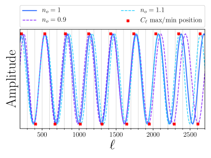
Frequency ($\omega$) Power-law index ($n_{o}$) Phase ($\varphi$) $14.6$ $1.1$ $0.5\pi$ $16.6$ $1.0$ $0.0$ $18.8$ $0.9$ $1.4\pi$

[table]parameters

Figure 2: Left: Oscillatory modulation of the power spectrum with a constant amplitude. In blue we see the fit for $n_{o}=1$, in light blue the one for $n_{o}=1.1$ and in purple for $n_{o}=0.9$. The red crosses are the positions of the maxima and minima of the acoustic peaks with the amplitude normalized to an arbitrary constant. See how even though $n_{o}=1$ offers a fairly good fit, the values of $n_{o}=1.1$ and $n_{o}=0.9$ respectively fit the maxima and the minima better. The fits to the frequency of the acoustic peaks have a fixed pivot multipole number at $\ell_{*}=814$. We note that the value of $\omega=16.6$ for $n_{o}=1$ at $k=0.0588{\rm Mpc}^{-1}$ agrees with the value $\omega=14.1$ used by Planck Akrami et al. (2018) at $k=0.05\,{\rm Mpc}^{-1}$. Right: Table containing the fit by eye values for template (1) used in Figure 2 on the left, the phase already being corrected by $\pi/2$ so that the oscillation is out of phase with the acoustic peaks.

We computed the effect of the feature (1) in the primordial power spectrum onto the lensed CMB temperature power spectrum using CLASS Lesgourgues (2011); Blas et al. (2011). We chose $H=100\,h{\rm km/s/Mpc}$, $h=0.67556$, $T_{\rm CMB}=2.7255{\rm K}$, $\Omega_{\rm b}h^{2}=0.02$, $\Omega_{\rm CDM}h^{2}=0.12$, $N_{\rm eff}=3.046$, $\Omega_{K}=0$, $\Omega_{\Lambda}=0.69$ and $A_{L}=1$. For the main power spectrum we took a power-law spectrum $P_{{\cal R},0}(k)=A_{s}\left(k/k_{\rm pivot}\right)^{n_{s}-1}$ with $A_{s}=2.2\cdot 10^{-9}$, $n_{s}=0.962$ and $k_{\rm pivot}=0.05{\rm Mpc}^{-1}$. For the oscillating feature we use the template (1) with the values presented in Table 2. In order to numerically implement a scale dependent amplitude with CLASS we have introduced an artificial cut-off at $k_{c}$ in the power spectrum, otherwise the spectrum eventually blows up for $n_{A}\neq 0$, so that our power-spectrum reads

$$P(k)=P_{{\cal R},0}(k)+\Delta P_{\cal R}(k)\times\left(1+\tanh\left[\beta\log(k/k_{c})\right]\right)/2\,,$$ (3)

and we respectively used $k_{c}=0.001\,{\rm Mpc}^{-1}$ ($\ell\sim 14$) and $\beta=10$ for $n_{A}<0$ and $k_{c}=1{\rm Mpc}^{-1}$ and $\beta=-10$ for $n_{A}>0$. For the oscillations in $k$, we further chose $n_{o}=1$, $\omega=16.6$ and $A=0.01$, except for the illustrative case where we considered $A=0.1$. It should be noted that this artificial cut-off introduced in this section will not be necessary when we study concrete inflationary models. The results can be seen in Fig. 3. On the left, we plotted an illustrative case with $A=0.1$ and we see that the oscillations do not exactly mimick the effect of smoothing (compare with Fig. 1) but it could be enough at the level of the residuals. On the right, we plotted the residuals between the lensed temperature power specturm with and without the oscillation for three different cases: $n_{A}=\{-1,0,1\}$. As one can see the residuals for $n_{A}=1$ are the ones that best resemble the residuals from the Planck 2018 analysis Aghanim et al. (2018), in particular for $\ell>814$. From the data, it seems that $n_{A}>0$ will be preferred but it is unclear how one could generate a growing feature, rather a decaying feature is expected from inflationary dynamics as we shall see in the next section. It should be noted that the apparent power loss in Fig. 3 is due to the enhancement of the contribution of density peaks (corresponding to peaks in the power spectrum) relative to velocity (Doppler) peaks (corresponding to troughs in the power spectrum) to temperature fluctuations Hu (1995). Thus, for the same initial conditions, the peaks in the power spectrum have a larger contribution from the oscillatory feature than the troughs.

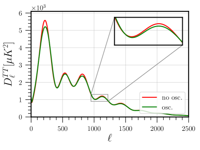
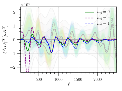
Figure 3: CMB lensed power spectrum and residuals for $\omega=16.6$, $n_{o}=1$ and $k_{*}=0.0588{\rm Mpc}^{-1}$ ($\ell_{*}=814$). On the left we compare the lensed power spectrum with and without the oscillations, respectively in green and red. We chose $n_{A}=0$ and $A=0.1$ so that the effects are clearer. In general, it does not mimick the smoothing effect of lensing. On the right, we compare the residuals between the lensed power spectrums (with and without oscillations) for three values of $n_{A}=\{-1,0,1\}$ with $A=0.01$ so that all of them have the same amplitude at $\ell_{*}$. For easier comparison, we have included in lower opacity Fig. 24 from Ref. Aghanim et al. (2018) as a background. In that image, we see in black the residuals of the $\Lambda$CDM model and the gray lines indicate the 1, 2, 3$\sigma$ countours. The green shadows refer to different values of $\Omega_{m}\,h^{2}$ which are not relevant for the present discussion. The red-orangish dotted line is the remaining residuals if there were $10\%$ more lensing. Compare our results (blue, green and purple) with the Planck residuals. Note how in the range $\ell\sim 1200-2000$ the two lines (black and red-orangish from Planck) are similar and follow the frequency of the acoustic peaks. Now, we see that the oscillations in Eq. (1) that could potentially resemble the Planck residuals Aghanim et al. (2018) is the one with $n_{A}>0$, since the peaks at large $\ell$ do not decay that fast.

III Features during inflation

In this section, we review the computation of the primordial power spectrum when there is a feature, e.g., sharp transition or oscillations, in the background evolution. In fact, such features are rather common in extensions of the simplest models of inflation. For example, it could be due to wiggles in the inflaton potential, inspired from axion monodromy in string theory Silverstein and Westphal (2008); Flauger et al. (2010), or sudden turns in the trajectory in field space in multi-field inflation Gao et al. (2013), which would excite the heavy modes. These features will affect the background dynamics during inflation and the effects will be imprinted in modifications of the slow-roll parameters and/or the sound speed of perturbations. Now, for simplicity, we take an effective single field approach Achucarro et al. (2011b); Shiu and Xu (2011); Achucarro et al. (2012); Bartolo et al. (2013); Palma (2015) and we study the resulting oscillatory modulation of the power spectrum. Our starting point is then the Mukhanov-Sasaki equation for the canonically normalized curvature perturbation Kodama and Sasaki (1984); Mukhanov et al. (1992):

$$u_{k}^{\prime\prime}+\left(c_{s}^{2}k^{2}-\frac{z^{\prime\prime}}{z}\right)u_{k}=0\,,$$ (4)

where $z^{2}\equiv 2a^{2}\epsilon M_{\rm pl}^{2}/c_{s}^{2}$, $a$ is the scale factor, $\epsilon\equiv-\dot{H}/H^{2}$, $H\equiv\dot{a}/a$, $c_{s}^{2}$ is the sound speed of propagation, $\dot{\,}\,\equiv d/dt$ where $t$ is the cosmic time, ${}^{\prime}\,\,\equiv d/d\tau$ where $d\tau=dt/a$ is the conformal time and $u\equiv z{\cal R}$ with ${\cal R}$ being the comoving curvature perturbation. We then consider the effect of a deviation in a de-Sitter inflationary background by introducing Achucarro et al. (2014)

$$v_{k}\equiv\sqrt{2kc_{s}}u_{k}\quad{\rm and}\quad f\equiv 2\pi zc_{s}^{1/2}\xi$$ (5)

where $d\xi=c_{s}d\tau$. With these redefinitions, Eq. (4) becomes Achucarro et al. (2014)

$$\frac{dv_{k}}{d\xi}+\left(k^{2}-\frac{2}{\xi^{2}}\right)v_{k}=\frac{1}{\xi^{2}f}\left(\frac{d^{2}f}{d\ln\xi^{2}}-3\frac{df}{d\ln\xi}\right)v_{k}\,.$$ (6)

Treating the right hand side as a perturbation one can solve the differential equation by the Green’s function method at leading order in $f$ by Gong and Stewart (2001); Joy et al. (2005); Gong (2005); Bartolo et al. (2013); Achucarro et al. (2014)

$$\frac{\Delta P_{\cal R}(k)}{P_{{\cal R},0}}=\int_{-\infty}^{\infty}d\ln\xi\,W(k\xi)\,\left(\frac{2}{3}\frac{d^{2}\ln f}{d\ln\xi^{2}}-2\frac{d\ln f}{d\ln\xi}\right)$$ (7)

where we already used the dS approximation, i.e. $v_{k}=\left(1-\frac{i}{k\xi}\right){\rm e}^{-ik\xi}$, we defined

$$P_{\cal R}(k)\equiv\frac{k^{3}}{2\pi^{2}}|v_{k}|^{2}\quad{\rm where}\quad P_{{\cal R},0}(k)\equiv\frac{1}{8\pi^{2}}\frac{H^{2}}{\epsilon c_{s}M_{\rm pl}^{2}}\,,$$ (8)

and

$$W(k\xi)\equiv\frac{3}{2}\left[\frac{\sin 2k\xi}{(k\xi)^{3}}-\frac{2\cos 2k\xi}{(k\xi)^{2}}-\frac{\sin 2k\xi}{k\xi}\right]\,.$$ (9)

This will be our starting point in the following discussions. Any feature during inflation will be contained in the function $f(\xi)$. Thus, once we know the type of feature we can compute its effect in the power spectrum by using Eq. (7) through modifications of the slow-roll parameters or the propagation speed. Interestingly, one can invert this relation and find the feature given a power-spectrum modulation as in Ref. Joy et al. (2005) (also see Ref. Durakovic et al. (2019) for a more recent approach). At this point, we could find the change in the background that would lead to the desired feature in the power spectrum. However, we will be more interested in the physical model behind. We will analytically compute three different regimes: $(i)$ fast oscillating features, $(ii)$ slow oscillating features and $(iii)$ sharp features. Here we do not seek to join any of these three regimes, rather we are interested to see if the desired oscillations in the power spectrum fall in any of these three categories.

III.1 Fast Oscillating feature

We begin to review the effects of an oscillating modulation of the background where its frequency is higher than the expansion rate. This could be either induced by an oscillatory modulation of the inflaton’s potential or by the oscillations of an extra massive field. For the moment, we will assume that the oscillations vary in amplitude and frequency and that $c_{s}=1$. Thus, in practice we have that

$$\frac{\Delta P_{\cal R}(k)}{P_{{\cal R},0}}=\frac{2}{3}\int_{-\infty}^{\infty}d\ln\tau\,W(k\tau)\,\frac{\Delta\left(\tau\right)}{H^{2}}$$ (10)

where we assumed that the frequency of the oscillation, say $\Omega$, in the function $f$ is $\dot{\Omega}/H=\delta_{\Omega}\Omega\gg 1$ then only the highest time derivative dominates and so

$$\frac{\Delta(\tau)}{H^{2}}\equiv\frac{d^{2}\ln f}{d\ln\tau^{2}}=-C(\tau)\cos\left[\Omega(\tau)+\varphi\right]\,,$$ (11)

with $\varphi$ being an arbitrary phase. For simplicity, we will further assume that

$$C(\tau)=C_{r}\left(\frac{a}{a_{r}}\right)^{\delta_{C}}\qquad{\rm and}\qquad\Omega(\tau)=\Omega_{r}\left(\frac{a}{a_{r}}\right)^{\delta_{\Omega}}\,,$$ (12)

where $a_{r}$ is the scale factor at onset of the resonance, $C_{r}$, $\Omega_{r}$, $\delta_{C}$, $\delta_{\Omega}$ are constants and we require $\dot{\Omega}/H=\delta_{\Omega}\Omega\gg 1$. Then, we can use the saddle point approximation for subhorizon scales ($k\tau\gg 1$) in Eq. (10) at $k=\delta_{\Omega}aH\Omega$ to find that the correction to the power-spectrum is given by

$$\frac{\Delta P_{\cal R}(k)}{P_{{\cal R},0}}\approx\sqrt{2\pi}\frac{C_{r}\left(\left|\delta_{\Omega}\right|\Omega_{r}\right)^{-3/2}}{\sqrt{|1-\delta_{\Omega}|}}\left(\frac{k}{k_{r}}\right)^{\frac{\delta_{C}-3\delta_{\Omega}/2}{1+\delta_{\Omega}}}\sin\left[\Omega_{r}\left(1+\delta_{\Omega}\right)\left(\frac{k}{k_{r}}\right)^{\frac{\delta_{\Omega}}{1+\delta_{\Omega}}}+\tilde{\varphi}\right]$$ (13)

where $k_{r}=\delta_{\Omega}\Omega_{r}a_{r}H_{r}$ and $\tilde{\varphi}=\varphi\mp\frac{3\pi}{4}$ where $-$ is for $\delta_{\Omega}>1$ and $+$ for $\delta_{\Omega}<1$.

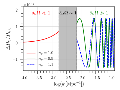
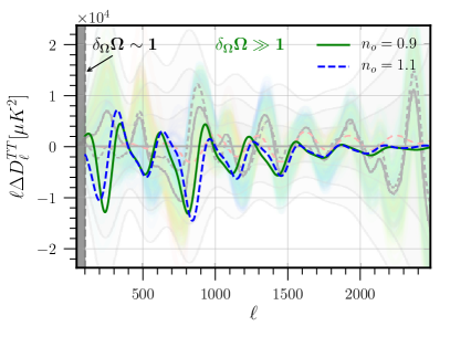
Figure 4: Left: Power spectrum modulation for the fast ($\delta_{\Omega}\Omega\gg 1$) and slow ($\delta_{\Omega}\Omega\ll 1$) oscillating regimes separated by an intermediate regime where numerical computations are needed (from $\delta_{\Omega}\Omega\sim 1/2$ to $\sim 2$). For the fast oscillating regime we chose $\delta_{\Omega}=9$ (green line), $\delta_{\Omega}=-11$ (dashed blue line) both cases with $\delta_{C}=3\delta_{\Omega}/2$ in Eq. (13) which corresponds to $n_{A}=0$ and $n_{o}=0.9$ and $n_{o}=1.1$ respectively in Eq. (1). For the slow oscillating regime (red line) we chose $\delta_{\Omega}=1$ and $\delta_{B}=0$ in Eq. (21) which corresponds to $n_{A}=0$ and $n_{o}=1$ in Eq. (1). In all cases we used Tab. 2 for the values of the frequency and phase. Right: Residuals of the lensed power spectrum for the same cases than in the left figure. For comparison, we included Fig. (24) of Planck analysis Aghanim et al. (2018). In black we have the residuals of the $\Lambda$CDM model, gray lines are the 1, 2, 3$\sigma$ countours and the green shadows refer to different values of $\Omega_{m}\,h^{2}$. The red-orangish dotted line is the remaining residuals if there were $10\%$ more lensing.

In order to compare with the data, we rewrite the parameters in Eq. (13) in terms of the template Eq. (1). Comparing them at a scale $k=k_{*}$ we find that for the frequency we have

$$\Omega_{r}={\omega}{\left|1-n_{o}\right|}\left(\frac{k_{r}}{k_{*}}\right)^{n_{o}}\quad{\rm,}\quad\delta_{\Omega}=\frac{n_{o}}{1-n_{o}},$$ (14)

and for the amplitude

$$C_{r}=\frac{A}{\sqrt{2\pi}}\left(\omega n_{o}\right)^{3/2}\left(\frac{k_{r}}{k_{*}}\right)^{3n_{o}/2}\sqrt{\left|\frac{1-2n_{o}}{1-n_{o}}\right|}\quad{\rm,}\quad\delta_{C}=\frac{n_{A}+3n_{o}/2}{1-n_{o}}\,.$$ (15)

First of all, we see that an exact linear dependence in $k$ for the frequency, as needed to fit all the acoustic peaks, is not possible: as $n_{o}\to 1$ we have that $\delta_{\Omega}\to\pm\infty$. This is because one would need that the resonance with every mode function, which has a frequency of $2k\xi$, occurred at the same time for all the modes, i.e. at $\xi=\xi_{r}$. Nevertheless, the best one can do without considering a sharp feature is that the oscillating source term oscillates so fast that the resonances occur almost at the same time. For this reason, we may consider that $n_{o}=\{0.9,1.1\}$ and the fit is still reasonable, see Fig. 4. However, while they might be give feasible residuals to mimick the smoothing effect of lensing, they are unsatisfactory from a theoretical point of view.

First of all, it must be seen whether the assumption $\delta_{\Omega}\Omega\gg 1$ holds for the range of interest. Plugging in some numbers (see Tab. 2), we find that

$$\delta_{\Omega}\Omega_{r}={n_{o}\omega}\left(\frac{k_{r}}{k_{*}}\right)^{n_{o}}\approx 1.7\times 10^{-1}\frac{n_{o}\omega}{16.6}\left(\frac{k_{r}}{10^{-2}k_{*}}\right)^{n_{o}}\,,$$ (16)

where we used the fact that $n_{o}\approx 1$. We see that, using the values of the frequencies in Tab. 2, the condition $\delta_{\Omega}\Omega\gg 1$ breaks down at around $k\sim 0.0035$ ($\ell\sim 49$) and so this kind of resonance could explain the anomaly down to small $\ell$. However, to be able to predict what occurs for $\ell<49$, as it enters the observational window, we need a full detailed model. For instance, it would difficult to imagine a model where the modulation suddenly started at $k\sim 0.0035$ since it would be accompanied by a sharp feature which usually has an amplitude higher relative to the fast oscillating regime and quite model dependent Chen et al. (2015).

Second and most important, we need to see if it is theoretically viable. To be close to a constant frequency we chose $n_{o}=\{0.9,1.1\}$ in Eq. (1) which correspond to $\delta_{\Omega}=\{9,-11\}$ in Eq. (13). This implies that the value of the frequency respectively increases or decreases 4 orders of magnitude in $1$ e-fold. In this respect, it is difficult to conceive what kind of model could sustain such growth or decay for more than the $3$ e-folds required. For example, in models where the feature is generated by an extra oscillating massive field like in Refs. Chen (2012); Huang and Pi (2018); Domènech et al. (2019), the frequency of the oscillation is associated to the mass of the field. In this case, either the energy density of the field increases too fast with the mass ($\delta_{\Omega}=9$) or it decreases so fast ($\delta_{\Omega}=-11$) that initially it should have had an astoundingly big mass and energy density. See App. A for a detailed comparison with such models. It should be noted that perhaps it may be possible to build such a model but we consider the amount of fine tuning required to be unreasonable. For these reasons, we will explore other simpler cases.

We thus disregard the fast oscillating case as a theoretically viable explanation for the $A_{L}$ anomaly. Nevertheless, it must be seen whether relaxing the assumption that the frequency be almost constant helps finding a viable model which resembles the lensing effect in a narrower multipole number range.

III.2 Slow Oscillating feature

In this subsection, we study the opposite case where the oscillating modulation is slowly varying. Thus, this feature will simply act as a modulation of the background and we can estimate its effects onto the power spectrum using the $\delta N$ formalism Starobinsky (1985); Salopek and Bond (1990); Sasaki and Stewart (1996). We have

$$\delta N=\frac{\partial N}{\partial\phi}\delta\phi+...$$ (17)

where $\frac{\partial N}{\partial\phi}=-\frac{H}{\dot{\phi}}$ is to be evaluated at horizon crossing. In general one has that $\langle\delta\phi\delta\phi\rangle=H/(2\pi c_{s})$ and so the power spectrum is given by

$$P_{{\cal R}}=\left(\frac{\partial N}{\partial\phi}\right)^{2}\langle\delta\phi\delta\phi\rangle=\frac{1}{8\pi^{2}}\frac{H^{2}}{\epsilon c_{s}M_{\rm pl}^{2}}\,.$$ (18)

The effect of any slow varying modulation of the background can be computed in this way, evaluated at horizon crossing $k=aH$. Now, let us assume that the modulation of the background results in a modulation of the slow-roll parameter given by

$$\epsilon=\epsilon_{0}\left(1-B(\tau)\sin\left[\Omega(\tau)+\varphi\right]\right)\,.$$ (19)

Assuming for simplicity that

$$B(\tau)=B_{r}\left(\frac{a}{a_{r}}\right)^{\delta_{B}}\qquad{\rm and}\qquad\Omega(\tau)=\Omega_{r}\left(\frac{a}{a_{r}}\right)^{\delta_{\Omega}}\,,$$ (20)

where $B_{r}$, $\Omega_{r}$, $\delta_{B}$ and $\delta_{\Omega}$ are constants, together with the requirement that $\delta_{\Omega}\Omega\ll 1$, we find that the modulation of the power-spectrum reads

$$\frac{\Delta P_{\cal R}(k)}{P_{{\cal R},0}}\approx B_{r}\left(\frac{k}{k_{r}}\right)^{\delta_{B}}\sin\left[\Omega_{r}\left(\frac{k}{k_{r}}\right)^{\delta_{\Omega}}+\varphi\right]\,.$$ (21)

Comparing this result with the template (1) we find

$$\Omega_{r}=\omega\frac{k_{r}}{k_{*}}\quad,\quad\delta_{\Omega}=n_{o}\quad,\quad B_{r}=A\quad{\rm and}\quad\delta_{B}=n_{A}\,.$$ (22)

This time, we have that for $\delta_{\Omega}=n_{o}=1$ at $k_{r}=10^{-2}k_{*}$, the oscillations are slowly varying, i.e. $\delta_{\Omega}\Omega_{r}\approx 1.7\times 10^{-1}$. However, since the frequency is increasing with time as a power-law of $a$, the approximation of $\delta_{\Omega}\Omega\ll 1$ will break down at around $\ell\sim 49$. This is clearly not enough to explain the lensing anomaly at $\ell\sim 1000-2000$. We will not attempt to join the slow and fast regimes of Sec. III.1, as it is not clear how to go from $\delta_{\Omega}\Omega\ll 1$ to $\delta_{\Omega}\Omega\gg 1$ smoothly and, furthermore, numerical computations would be needed.

III.3 Sharp feature

When one considers a sharp feature, the exact shape of the modulation is very model dependent Starobinsky (1992); Adams et al. (2001); Choe et al. (2004); Gong (2005); Dvorkin and Hu (2010); Achucarro et al. (2011a); Adshead et al. (2012); Shiu and Xu (2011); Gao et al. (2013); Bartolo et al. (2013); Palma (2015). Nevertheless, let us consider the simplest example where the sharp feature is a discontinuity, e.g. a step in the slope of the potential, which will result in a Dirac delta $\delta(\xi-\xi_{f})$ in Eq. (7), as the slow roll parameter $\epsilon$ in $f(\xi)$ is proportional to the first derivative of the potential. In that case, the frequency of the resulting oscillation will be proportional to $2k\xi_{f}$ Gong and Stewart (2001); Joy et al. (2005); Gong (2005). A quick exercise tells us that if we require $\omega=16.6$ the transition happened at $k_{*}\xi_{r}\approx 8.3$, that is the transition happened $2$ e-folds before our pivot scale at around $k_{f}\approx 0.007{\rm Mpc}^{-1}$ or $\ell_{r}\approx 98$. Furthermore, the phase of the oscillation depends on whether the step around $\xi=\xi_{f}$ is odd (e.g. a hyperbolic tangent) Starobinsky (1992); Choe et al. (2004); Gong (2005); Bartolo et al. (2013) or even (e.g. a gaussian bump) Achucarro et al. (2014). To understand that it is useful to integrate by parts Eq. (7) arriving at

$$\frac{\Delta P_{\cal R}(k)}{P_{{\cal R},0}}=-2\int_{-\infty}^{\infty}d\ln\xi\,\left(W(k\xi)+\frac{1}{3}\frac{dW(k\xi)}{d\ln\xi}\right)\,\frac{d\ln f}{d\ln\xi}\,.$$ (23)

If the step is sharp enough only the neighborhood of the transition will contribute to the integral. If the step is odd around $\xi=\xi_{f}$, its derivative is even and so the even function $\cos(2k\xi_{f})$ survives asymptotically in $k$. Instead, if the step is even around $\xi=\xi_{f}$, then its derivative is odd and the odd function $\sin(2k\xi_{f})$ remains.

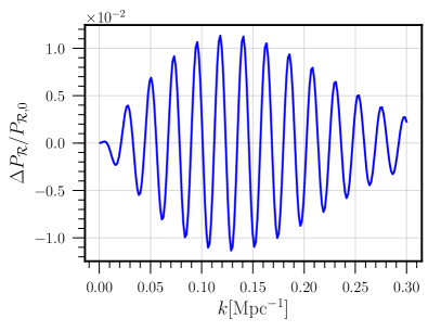
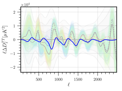
Figure 5: Power spectrum modulation (25) (left) and residuals of the lensed power spectrum (right) for a bump (24) in $c_{s}^{2}$ with height $B=-0.015$ and sharpness $\beta_{s}=25$. Note that on the right the residuals are similar to those in the Planck analysis Aghanim et al. (2018) Fig. (24), which we included for easier comparison. Again, we have in black the residuals of the $\Lambda$CDM model, the gray lines are the 1, 2, 3$\sigma$ countours and the green shadows refer to different values of $\Omega_{m}\,h^{2}$. The red-orangish dotted line is the remaining residuals if there were $10\%$ more lensing. Compare our result (blue) with the Planck residuals (black and red-orangish). Note also that although the frequency of our resulting oscillations have a similar pattern, the amplitude of the Planck residuals are shifted upwards compared to our result.

We present now a concrete example. The simplest case is a bump in the sound speed at $\tau=\tau_{f}$ with height $B$ and sharpness $\beta_{s}$ given by Achucarro et al. (2014)

$$c_{s}^{2}=1+B{\rm e}^{-\beta_{s}^{2}\log^{2}\left[\tau/\tau_{f}\right]}\,.$$ (24)

Note that if $B>0$ the sound speed of scalar perturbations is slightly superluminal. Although it does not pose any causality problems Babichev et al. (2008), it may obstruct the UV completion of a quantum Lorentz-invariant theory Adams et al. (2006). Nevertheless, the superluminality could be compensated by introducing a $c^{2}_{s,0}$ as a common factor in Eq. (24) with $(1+B)c^{2}_{s,0}\leq 1$. Now, integrating Eq. (23) under the assumption that the step is sharp ($\beta_{s}\gg 1$) yields Achucarro et al. (2014) (see also App. B)

$$\frac{\Delta P_{\cal R}(k)}{P_{{\cal R},0}}=B\sqrt{\pi}\frac{k\tau_{f}}{\beta_{s}}{\rm e}^{-\frac{k^{2}\tau_{f}^{2}}{\beta_{s}^{2}}}\left\{\sin(2k\tau_{f})+\frac{\cos(2k\tau_{f})}{k\tau_{f}}-\frac{1}{2}\frac{\sin(2k\tau_{f})}{(k\tau_{f})^{2}}\right\}\,,$$ (25)

where we neglected terms $O(\beta_{s}^{-2})$ and note that $\Delta P_{\cal R}\to 0$ when $k\to 0$ so that there are no spurious super-horizon modes. To estimate the magnitude of the feature, note that the gaussian modulation has a maximum at $k\tau_{f}=\beta_{s}/\sqrt{2}$ and so to have an amplitude of $10\%$ one needs $|B|\approx 0.013$. It should be noted that the tensor-to-scalar ratio , which is proportional to $c_{s}$ Mukhanov and Vikman (2006), is barely affected as the sound speed only changes by $10\%$. Furthermore, the adiabatic condition $s\equiv\dot{c}_{s}/Hc_{s}$ is always satisfied and its maximum value is $|s|=|B|\beta_{s}/\sqrt{2e}\approx 0.16$ (for $|B|=0.015$ and $\beta_{s}=25$). We have plotted the oscillatory feature in the primordial power spectrum and the residuals of the lensed power spectrum in Fig. 5. Note how the frequency of the resulting oscillatory pattern follows that of Planck Aghanim et al. (2018) in the range $\ell\sim 1200-2000$, although the residuals from Planck are slightly shifted upwards.

Regarding the non-gaussianities we can borrow the results from Ref. Achucarro et al. (2014) (see also App. C) at the equilateral limit and find that the equilateral non-gaussianity peaks at $K\tau_{f}=\sqrt{6}\beta_{s}$ with amplitude

$$f_{NL}^{\rm eq}\approx-0.27\,B\beta_{s}^{2}\,.$$ (26)

A similar calculation for the trispectrum evaluated at its peak ($K\tau_{f}=\sqrt{10}\beta_{s}$) in the equilateral configuration (see App. C) yields

$$g^{\rm eq}_{NL}\approx-0.1\,B\beta_{s}^{4}\,.$$ (27)

The Planck results on non-gaussianities Ade et al. (2016) yield that $f_{NL}^{\rm eq}=-4\pm 43$. Thus, if $|B|\sim 10^{-2}$ we see that we need $\beta_{s}<60$ to fall within the bounds. Regarding local (squeezed shape) non-gaussianity its magnitude is at least suppressed by $1/\beta_{s}$ with respect to $f_{NL}^{\rm eq}$ Achúcarro et al. (2013); Mooij et al. (2016) and therefore we easily fall within Planck constraints, i.e. $f_{NL}^{\rm loc}=0.8\pm 5.0$. Note that these constraints are looser if one allows for a scale dependence in the non-gaussianity Ade et al. (2016). Furthermore, the constraints on the trispectrum are roughly Ade et al. (2016) $g_{NL}<10^{5}-10^{6}$ and for $|B|\sim 10^{-2}$ it is sufficient that $\beta_{s}<100$. Thus, as we can see in Fig. 5 a bump in $c_{s}^{2}$ with $B=-0.015$ and $\beta_{s}=25$ reproduces quite well the residuals in the Planck analysis Aghanim et al. (2018) and is well within the bispectrum and trispectrum bounds. The development of a specific model that can produce such a bump in $c_{s}^{2}$ is left for future work, although it seems possible to build such a model using a spectator scalar field Nakashima et al. (2011). Before ending this section, it is worth saying that no trans-planckian modulation Easther et al. (2005) could mimick the smoothing effect of lensing. This is due to the fact that the value of the frequency for trans-planckian modulations depends on the initial conditions but the frequency required to explain the anomaly correspond to a scale in the last few e-folds of inflation.

IV Conclusions

The latest analysis of the cosmic microwave background by the Planck team Aghanim et al. (2018) suggests that at the $2\sigma$ confidence level there is $10\%$ more lensing than predicted by $\Lambda$CDM. If not a statistical fluke, one suggested explanation for the extra lensing is that there is new physics that mimicks the smoothing effect of lensing Akrami et al. (2018). Here we studied what could have generated these oscillations in the power spectrum during inflation. We first considered an effective single field approach, where the effects of a sharp transition or an oscillatory modulation in the background can be studied phenomenologically Shiu and Xu (2011); Achucarro et al. (2012); Bartolo et al. (2013); Palma (2015). In this way, we divided the analysis between rapid/slow (compared to the expansion rate) oscillatory modulations and sharp transitions.

We have found that for rapid oscillatory modulations Chen (2012); Huang and Pi (2018); Domènech et al. (2019), it is not possible to obtain an exact linear $k$ dependence in the frequency of the power-spectrum’s oscillations since the modulation should oscillate infinitely fast or be a sharp feature. Nevertheless, an almost linear dependence can be obtained for very fast oscillatory modulations. Unfortunately, when compared with the data one needs a frequency which is slowly varying for large scales ($\ell<50$) and rapidly varying for $\ell>50$. We also showed that if the oscillations were caused by an oscillating heavy field, then the mass of the field would have been smaller than Hubble at some point in the range of interest. Thus, this sort of feature cannot explain an oscillation over the whole range of $\ell$ covered by the Planck data. We discussed that the possibility of starting the oscillation at $\ell>50$ is not feasible since it would be accompanied by a sharp feature which is normally larger than the oscillatory feature.

On the other hand, we have analyzed the case of slowly oscillating modulations of the background and we have found that it is possible to find a model where the frequency of the oscillatory feature is linear in $k$. In this case, there is no resonance occurring and so the frequency must evolve inversely proportional to the conformal time so that at horizon crossing ($-k\tau\approx 1$) yields a linear dependence in $k$. However, when compared with the data and in agreement with the results of fast oscillatory modulations, this feature could only explain a linear oscillation for $\ell<50$ which is not of interest for our work.

Motivated by our results, we have studied sharp transitions within an effective single field theory for sharp features Shiu and Xu (2011); Achucarro et al. (2012); Bartolo et al. (2013); Palma (2015). When the feature is sharp all the modes are excited at the same time (say $\tau=\tau_{f}$) and so the resulting oscillatory feature has a frequency of $2k\tau_{f}$. If that is the case, we needed that the sharp feature occurred at scales inside the observational window, around $\ell\sim 98$. Although sharp features are very model dependent Starobinsky (1992); Adams et al. (2001); Choe et al. (2004); Gong (2005); Dvorkin and Hu (2010); Achucarro et al. (2011a); Adshead et al. (2012); Shiu and Xu (2011); Gao et al. (2013); Bartolo et al. (2013); Palma (2015), we see that in general terms when the sharp feature is even Achucarro et al. (2014), e.g. a bump, the oscillations with the right frequency are in phase with the acoustic peaks. We have presented an example capable of reproducing the desired oscillatory modulation of the primordial power spectrum times a damping function (25). This example consists of a bump in the sound speed given by Eq. (24). Moreover, we have shown that this model can satisfy the bounds to the bispectrum and trispectrum.

We thus conclude, on one hand, that the $A_{L}$ anomaly in the CMB temperature power spectrum could potentially be explained by a bump in the sound speed of scalar perturbations, although a detailed comparison with the data would be needed. We presented the residuals in Fig. 5 and they are similar in frequency to the results presented in Ref. Aghanim et al. (2018). In the future, measurements of baryon acoustic oscillations might be employed in combination with the CMB Zeng et al. (2019) to test this explanation. In the standard scenario, the Fourier wavenumbers for the peaks in the late-time matter power spectrum are shifted relative to those for peaks in the radiation density at CMB decoupling Eisenstein and Hu (1998), a result of the fact that the late-time growing mode maps at early times to a combination of the growing and decaying modes. The relative phases of the acoustic and primordial oscillations will thus be different in the baryon acoustic oscillations (BAO) than they are in the CMB. It will be interesting do this analysis with high precision polarization data such as CMB-S4. Furthermore, another probe of this model would be to look for correlated features in the primordial spectra Achúcarro et al. (2013); Gong et al. (2014); Chen et al. (2016b); Finelli et al. (2018); Ballardini et al. (2016, 2018); Palma et al. (2018); Gong et al. (2017). On the other hand, we have shown also that it is difficult that oscillating features in the power spectrum which are linear in $k$ (or almost linear) are generated during inflation from an oscillatory modulation of the background and that could explain the $A_{L}$ anomaly at the same time. However, it has to be seen if there is any possibility for general multi-field inflationary trajectories as in Ref. Gao et al. (2013).

Appendix A Model building

In this section we give the phenomenological parameters in Sec. III in terms of particular models. We will first consider a two-field model in which the heavy field is excited and oscillates around the minimum of its potential. This could be a particular realization of the case studied in Sec. III.1 as the heavier the field the faster the oscillations. In the second example, we will consider that the inflaton’s potential has an oscillatory modulation superimposed. This could be an example for either fast or slow oscillations depending on the model parameters and could be used in Secs. III.1 and III.2.

A.1 Non-standard clock signal

Here we review the model studied in Domènech et al. (2019) which is a generalized version of the standard clock model proposed in Ref. Chen (2012). The action is given by

$$S=\int\mathop{d^{4}x}\sqrt{-g}\Bigg{\{}\frac{M_{\rm pl}^{2}}{2}R-\frac{1}{2}\left(1+\frac{\sigma}{\Lambda}\right)^{2}g^{\mu\nu}\partial_{\mu}\phi\partial_{\nu}\phi-\frac{1}{2}f^{2}(\phi)g^{\mu\nu}\partial_{\mu}\sigma\partial_{\nu}\sigma-V(\phi)-\frac{1}{2}m(\phi)^{2}\sigma^{2}\,.\Bigg{\}}\,.$$ (28)

Assuming that the $\sigma$ field is massive, does not spoil slow-roll inflation and does not backreact on the equations of motion for $\phi$ we have that $\sigma$ oscillates around the minimum of the effective potential given by the centrifugal force by

$$\Delta\sigma=\Delta\sigma_{r}\left(\frac{a}{a_{r}}\right)^{-3/2}\frac{f_{r}}{f}\sqrt{\frac{m_{\rm eff,r}}{m_{\rm eff}}}\Big{\{}\cos\left(\int_{t_{r}}^{t}m_{\rm eff}\,dt\right)+O(1/\mu)\Big{\}}$$ (29)

where $m_{\rm eff}^{2}={m^{2}}/{f^{2}}-{\ddot{f}}/{f}-3H{\dot{f}}/{f}$ and we will assume that the time derivatives of $f$ are negligible in front of $m$. All these conditions can be satisfied, at least momentarily, if the energy fraction of the massive field is smaller than the slow-roll parameter $\epsilon\equiv-\dot{H}/H^{2}$. Then, the leading interacting term is given by

$$\frac{\Delta(\tau)}{H^{2}}=\frac{\ddot{\sigma}}{H^{2}\Lambda}$$ (30)

which yields

$$C_{r}=\mu_{r}^{2}\frac{\Delta\sigma_{r}}{\Lambda}\quad\,,\,\quad\Omega_{r}=\frac{\mu_{r}}{\delta_{\Omega}}\,,$$ (31)

where $\mu_{r}\equiv\frac{m_{{\rm eff},r}}{H_{r}}$,

$$\delta_{C}=-\frac{3}{2}+\frac{3}{2}\delta_{m}-\frac{5}{2}\delta_{f}\quad{\rm and}\quad\delta_{\Omega}=\delta_{m}-\delta_{f}\,.$$ (32)

We have defined

$$\delta_{f}\equiv\frac{d\ln f}{dN}\quad{\rm and}\quad\delta_{m}\equiv\frac{d\ln m}{dN}\,,$$ (33)

where $dN=Hdt$.

For the values used in the main text (see Tab. 2) we have that the effective dimensionless mass and the amplitude of the field oscillation at the pivot scale respectively are

$$\mu_{*}=\omega n_{o}\sim 15\qquad{\rm and}\qquad\frac{\Delta\sigma_{*}}{\Lambda}\sim\mu_{*}^{-2}\sim 10^{-2}\,.$$ (34)

Thus, at the pivot scale the values are reasonable. However, we also require $|\delta_{\Omega}|\sim 10$ and this implies $\delta_{m},\delta_{f}\sim 10$. This model has a growth (or decay) of the mass and/or the coefficient of the kinetic term of 4 order of magnitude per e-fold. We conclude that either there is much fine-tuning in the potential or kinetic term or the extra field will backreact in few e-folds.

A.2 Oscillating potential

Let us consider that the inflaton potential has an oscillating modulation of the form

$$V=V_{0}(\phi)\left(1+W(\phi)\sin\left[\Omega(\phi)+\varphi\right]\right)\,.$$ (35)

In order not to spoil slow-roll, i.e. $\eta\equiv\frac{\dot{\epsilon}}{H\epsilon}\ll 1$ we need that $W\dot{\Omega}^{2}<1$. This can be tuned by an appropriate form of $W(\phi)$. Comparing with the results of Sec. III we find

$$\frac{\delta\epsilon}{\epsilon}\approx\frac{W}{2}\frac{\dot{\Omega}}{H}\cos\left[\Omega(\tau)+\varphi\right]$$ (36)

and so

$$\frac{\Delta(\tau)}{H^{2}}=\frac{\ddot{\delta}\epsilon}{2H^{2}\epsilon}$$ (37)

which yields

$$C_{r}=\frac{W_{r}}{4}\delta_{\Omega}^{3}\Omega_{r}^{3}\quad{\rm and}\quad\delta_{C}=\delta_{W}+3\delta_{\Omega}\,.$$ (38)

We have defined

$$\delta_{W}\equiv\frac{d\ln W}{dN}\quad{\rm and}\quad\delta_{\Omega}\equiv\frac{d\ln\Omega}{dN}\,.$$ (39)

Appendix B Estimation of the power spectrum

Here we give a brief review of the estimation for the power spectrum. The starting point is Eq.(7), which using the fact that $f\propto z\,c_{s}^{1/2}\propto c_{s}^{-1/2}$ and that $s\equiv\dot{c}_{s}/Hc_{s}$ reads

$$\frac{\Delta P_{\cal R}(k)}{P_{{\cal R},0}}\approx\int_{-\infty}^{\infty}d\ln\xi\,\left(\frac{\sin\left(2k\xi\right)}{k\xi}-\cos\left(2k\xi\right)\right)\,s(\xi)\,.$$ (40)

Now, using that

$$c_{s}^{2}=1+BF(\ln(\tau/\tau_{f}))\quad{\rm where}\quad F\equiv{\rm e}^{-\beta_{s}^{2}\ln^{2}\left(\tau/\tau_{f}\right)}\quad{,}\quad B\ll 1\quad{,}\quad\beta_{s}\gg 1\,,$$ (41)

and that $s=\frac{B\beta_{s}}{2}\frac{dF}{dx}$, where $x\equiv-\beta_{s}\ln\left(\tau/\tau_{f}\right)$, we can write at leading order in $x/\beta_{s}$

$$\frac{\Delta P_{\cal R}(k)}{P_{{\cal R},0}} \approx\frac{B}{2}{\rm Re}\left[\int_{-\infty}^{\infty}dx\frac{dF}{dx}\left(1+\frac{x}{\beta_{s}}\right){\rm e}^{2ikc_{s}\tau}\right]-\frac{B}{2}{\rm Re}\left[\int_{-\infty}^{\infty}dx\frac{dF}{dx}{\rm e}^{2ikc_{s}\tau}\right]$$

$$\approx B\sqrt{\pi}\frac{k\tau_{f}}{\beta_{s}}{\rm e}^{-\frac{k^{2}\tau_{f}^{2}}{\beta_{s}^{2}}}\left\{\sin(2k\tau_{f})+\frac{\cos(2k\tau_{f})}{k\tau_{f}}-\frac{1}{2}\frac{\sin(2k\tau_{f})}{(k\tau_{f})^{2}}\right\}\,,$$ (42)

where used that $\xi\approx\tau$ and we expanded the mode functions as

$${\rm e}^{ikc_{s}\tau}\approx{\rm e}^{ik\tau_{f}}{\rm e}^{-ik\tau_{f}x/\beta_{s}}\,,$$ (43)

since $\tau\approx\tau_{f}\left(1-\frac{x}{\beta_{s}}\right)$.

Appendix C Estimation of the bispectrum and trispectrum

Here we briefly derive the estimate for the magnitude of the bispectrum and trispectrum. We work in the effective field theory of inflation approach Cheung et al. (2008); Bartolo et al. (2013); Achucarro et al. (2014) and expand the action up to fourth order. By picking up the terms that only involve the speed of sound $c_{s}$ and its derivatives at leading order in slow roll we find

$${S}_{3}=\int dtd^{3}x{a^{3}}\frac{M_{\rm pl}^{2}\epsilon}{H}\left\{(1-c_{s}^{-2})\dot{\cal R}^{3}+2Hsc_{s}^{-2}\dot{\cal R}^{2}{\cal R}-a^{-2}(1-c_{s}^{-2})\dot{\cal R}\left(\partial{\cal R}\right)^{2}\right\}$$ (44)

and

$${S}_{4}=\int dtd^{3}x {a^{4}}\frac{M_{\rm pl}^{2}\epsilon}{4H^{2}}\Bigg{\{}-(1-c_{s}^{-2})\left[\dot{\cal R}^{2}-a^{-2}\left(\partial{\cal R}\right)^{2}\right]^{2}$$

$$-8Hsc_{s}^{-2}a^{-2}\left(\partial{\cal R}\right)^{2}\dot{\cal R}^{2}{\cal R}+\left(16H^{2}s^{2}-8H\dot{s}\right)c_{s}^{-2}\dot{\cal R}^{2}{\cal R}^{2}\Bigg{\}}\,.$$ (45)

We will use the approximation for sharp features which consists of expanding around the transition time Adshead et al. (2011, 2012); Bartolo et al. (2013); Achucarro et al. (2014).

C.1 Bispectrum

For the bispectrum we use the in-in formalism Maldacena (2003); Wang (2014),

$$\langle{\cal R}_{k_{1}}{\cal R}_{k_{2}}{\cal R}_{k_{3}}\rangle=-2i{\rm Re}\left[\int d\tau d^{3}x\langle{\cal R}_{k_{1}}{\cal R}_{k_{2}}{\cal R}_{k_{3}}H_{I,3}\rangle\right]$$ (46)

where $H_{I,3}=-{\cal L}_{3}$. As usual we use the de-Sitter mode function:

$${\cal R}_{k}=\frac{H}{\sqrt{4\epsilon c_{s,0}k^{3}}}\left(1+ikc_{s,0}\tau\right){\rm e}^{-ikc_{s}\tau}\,.$$ (47)

Now, picking up the highest contribution in terms of $\beta_{s}$ and evaluating the integral near the sharp feature and in the equilateral configuration ($k_{1}=k_{2}=k_{3}=k$ and $\mathbf{k_{1}}\cdot\mathbf{k_{2}}=-k^{2}/2$) we have

$$\langle{\cal R}_{k_{1}}{\cal R}_{k_{2}}{\cal R}_{k_{3}}\rangle^{\rm eq} \approx\frac{3}{4}B\beta_{s}^{2}{\rm Im}\Bigg{[}\int dx\,{\rm e}^{iKc_{s}\tau}\Big{(}F\left(\frac{k\tau}{\beta_{s}}\right)^{3}-\frac{1}{2}F\beta_{s}^{-2}\left(\frac{k\tau}{\beta_{s}}\right)\left(1-i{k\tau}\right)^{2}$$

$$-\frac{dF}{dx}\beta_{s}^{-1}\left(\frac{k\tau}{\beta_{s}}\right)\left(1-i{k\tau}\right)\Big{)}\Bigg{]}\times\frac{P_{{\cal R},0}^{2}M_{\rm pl}^{6}}{k^{6}}\left(2\pi\right)^{7}\delta(\mathbf{k_{1}}+\mathbf{k_{2}}+\mathbf{k_{3}})$$ (48)

$$\approx-\frac{\sqrt{\pi}}{3}B\beta_{s}^{2}\left(\frac{K\tau_{f}}{2\beta_{s}}\right)^{3}{\rm e}^{-\frac{K^{2}\tau_{f}^{2}}{4\beta_{s}^{2}}}\sin\left(K\tau_{f}\right)\times\frac{P_{{\cal R},0}^{2}M_{\rm pl}^{6}}{k^{6}}\left(2\pi\right)^{7}\delta(\mathbf{k_{1}}+\mathbf{k_{2}}+\mathbf{k_{3}})$$ (49)

where $K=k_{1}+k_{2}+k_{3}$ and $P_{{\cal R},0}=\frac{H^{2}}{8\pi^{2}\epsilon c_{s}M_{\rm pl}^{2}}$. With this result we find that

$$f_{NL}^{\rm eq}\approx-\frac{10\sqrt{\pi}}{27}B\beta_{s}^{2}\left(\frac{K\tau_{f}}{2\beta_{s}}\right)^{3}{\rm e}^{-\frac{K^{2}\tau_{f}^{2}}{4\beta_{s}^{2}}}\sin\left(K\tau_{f}\right)\,,$$ (50)

where we used that

$$\langle{\cal R}_{k_{1}}{\cal R}_{k_{2}}{\cal R}_{k_{3}}\rangle=\frac{3}{10}f_{NL}(k_{1},k_{2},k_{3})\frac{k_{1}^{3}+k_{2}^{3}+k_{3}^{2}}{k_{1}^{3}k_{2}^{3}k_{3}^{3}}P_{{\cal R},0}^{2}M_{\rm pl}^{6}\left(2\pi\right)^{7}\delta(\mathbf{k_{1}}+\mathbf{k_{2}}+\mathbf{k_{3}})\,.$$ (51)

C.2 Trispectrum

Again, for the trispectrum we will use the in-in formalism. However, this time we have the possibility of a scalar exchange Arroja and Koyama (2008); Chen et al. (2009); Wang (2014), i.e.

$$\langle{\cal R}_{k_{1}}{\cal R}_{k_{2}}{\cal R}_{k_{3}}{\cal R}_{k_{4}}\rangle_{SE} =\int d^{3}xd\tau{{}^{\prime}}\int_{-\infty}^{\tau}d\tau{{}^{\prime\prime}}\langle H_{I,3}(\tau^{\prime}){\cal R}_{k_{1}}{\cal R}_{k_{2}}{\cal R}_{k_{3}}{\cal R}_{k_{4}}H_{I,3}(\tau^{\prime\prime})\rangle$$

$$-\int d^{3}xd\tau{{}^{\prime}}\int_{-\infty}^{\tau^{\prime}}d\tau{{}^{\prime\prime}}\langle H_{I,3}(\tau^{\prime\prime})H_{I,3}(\tau^{\prime}){\cal R}_{k_{1}}{\cal R}_{k_{2}}{\cal R}_{k_{3}}{\cal R}_{k_{4}}\rangle$$

$$-\int d^{3}xd\tau{{}^{\prime}}\int_{-\infty}^{\tau^{\prime}}d\tau{{}^{\prime\prime}}\langle{\cal R}_{k_{1}}{\cal R}_{k_{2}}{\cal R}_{k_{3}}{\cal R}_{k_{4}}H_{I,3}(\tau^{\prime})H_{I,3}(\tau^{\prime\prime})\rangle\,$$ (52)

and a contact interaction Chen et al. (2009), that is

$$\langle{\cal R}_{k_{1}}{\cal R}_{k_{2}}{\cal R}_{k_{3}}{\cal R}_{k_{4}}\rangle_{CI}=-2i{\rm Re}\left[\int d\tau d^{3}x\langle{\cal R}_{k_{1}}{\cal R}_{k_{2}}{\cal R}_{k_{3}}{\cal R}_{k_{4}}H_{I,4}\rangle\right]\,.$$ (53)

However, a quick inspection of the scalar exchange contribution tells us that the contribution of the scalar exchange is proportional to $f_{NL}^{2}\approx B^{2}\beta_{s}^{4}$ since, at most, there are two cubic vertex proportional to $B\beta_{s}^{2}$. As we will now see, this contribution is suppressed by a factor $B$ with respect to the leading contribution of the contact interaction which is proportional to $B\beta_{s}^{4}$ – e.g. look at the term $\dot{s}$ in $S_{4}$ which will bring twice $\beta_{s}^{2}$ down.

Now, to simplify the computation of the interaction Hamiltonian we will assume that only the terms which are proportional to $(1-c_{s}^{2})$ contribute to the third order Lagrangian and, thus, the third order Lagrangian is only proportional to $B$. This means that the terms in the fourth order interaction Hamiltonian that come from ${\cal L}_{3}$ are always squared and so proportional to $B^{2}$. In this way, we can neglect the terms coming from ${\cal L}_{3}$ and ${\cal L}_{2}$ and the interaction Hamiltonian is, for our purposes, given by

$$H_{I,4}=-{\cal L}_{4}+O(B^{2}).$$ (54)

We again select the highest contribution in terms of $\beta_{s}$ and evaluate the integral near the sharp feature and in the regular tetrahedron configuration ($k_{1}=k_{2}=k_{3}=k_{4}=k$ and $|\mathbf{k_{1}}+\mathbf{k_{3}}|=|\mathbf{k_{2}}+\mathbf{k_{4}}|=k$). Then we find

$$\langle{\cal R}_{k_{1}}{\cal R}_{k_{2}}{\cal R}_{k_{3}}{\cal R}_{k_{4}}\rangle^{\rm eq} \approx-\frac{1}{2}B\beta_{s}^{4}{\rm Im}\Bigg{[}\int dx\,{\rm e}^{iKc_{s}\tau}\Big{(}\frac{1}{8}\left(\frac{k\tau}{\beta_{s}}\right)^{5}F+2i\left(\frac{k\tau}{\beta_{s}}\right)^{4}\frac{dF}{dx}-3\left(\frac{k\tau}{\beta_{s}}\right)^{3}\frac{d^{2}F}{dx^{2}}\Big{)}\Bigg{]}$$

$$\times\frac{P_{{\cal R},0}^{3}M_{\rm pl}^{8}}{k^{9}}\left(2\pi\right)^{9}\delta(\mathbf{k_{1}}+\mathbf{k_{2}}+\mathbf{k_{3}}+\mathbf{k_{4}})$$ (55)

$$\approx-\frac{321}{512}\sqrt{\pi}B\beta_{s}^{4}\left(\frac{K\tau_{f}}{2\beta_{s}}\right)^{5}{\rm e}^{-\frac{K^{2}\tau_{f}^{2}}{4\beta_{s}^{2}}}\sin\left(K\tau_{f}\right)\times\frac{P_{{\cal R},0}^{3}M_{\rm pl}^{8}}{k^{9}}\left(2\pi\right)^{9}\delta(\mathbf{k_{1}}+\mathbf{k_{2}}+\mathbf{k_{3}}+\mathbf{k_{4}})$$ (56)

where now $K=k_{1}+k_{2}+k_{3}+k_{4}$ and $P_{{\cal R},0}=\frac{H^{2}}{8\pi^{2}\epsilon c_{s}M_{\rm pl}^{2}}$. So we have

$$g^{\rm eq}_{NL}=-\frac{2675}{36864}\sqrt{\pi}B\beta_{s}^{4}\left(\frac{K\tau_{f}}{2\beta_{s}}\right)^{5}{\rm e}^{-\frac{K^{2}\tau_{f}^{2}}{4\beta_{s}^{2}}}\sin\left(K\tau_{f}\right)$$ (57)

where we used the normalization of Smith et al. (2015) in order to compare with Ade et al. (2016), that is

$$\langle{\cal R}_{k_{1}}{\cal R}_{k_{2}}{\cal R}_{k_{3}}{\cal R}_{k_{4}}\rangle=\frac{216}{100}g_{NL}(k_{1},k_{2},k_{3})\frac{k_{1}^{3}+k_{2}^{3}+k_{3}^{3}+k_{4}^{3}}{k_{1}^{3}k_{2}^{3}k_{3}^{3}k_{4}^{3}}\times P_{{\cal R},0}^{3}M_{\rm pl}^{8}\left(2\pi\right)^{9}\delta(\mathbf{k_{1}}+\mathbf{k_{2}}+\mathbf{k_{3}}+\mathbf{k_{4}})\,.$$ (58)

References

- Seljak (1996) Uros Seljak, “Gravitational lensing effect on cosmic microwave background anisotropies: A Power spectrum approach,” Astrophys. J. 463, 1 (1996), arXiv:astro-ph/9505109 [astro-ph] .
- Lewis and Challinor (2006) Antony Lewis and Anthony Challinor, “Weak gravitational lensing of the CMB,” Phys. Rept. 429, 1–65 (2006), arXiv:astro-ph/0601594 [astro-ph] .
- Hanson et al. (2010) Duncan Hanson, Anthony Challinor, and Antony Lewis, “Weak lensing of the CMB,” Gen. Rel. Grav. 42, 2197–2218 (2010), arXiv:0911.0612 [astro-ph.CO] .
- Aghanim et al. (2018) N. Aghanim et al. (Planck), “Planck 2018 results. VI. Cosmological parameters,” (2018), arXiv:1807.06209 [astro-ph.CO] .
- Calabrese et al. (2008) Erminia Calabrese, Anze Slosar, Alessandro Melchiorri, George F. Smoot, and Oliver Zahn, “Cosmic Microwave Weak lensing data as a test for the dark universe,” Phys. Rev. D77, 123531 (2008), arXiv:0803.2309 [astro-ph] .
- Muñoz et al. (2016) Julian B. Muñoz, Daniel Grin, Liang Dai, Marc Kamionkowski, and Ely D. Kovetz, “Search for Compensated Isocurvature Perturbations with Planck Power Spectra,” Phys. Rev. D93, 043008 (2016), arXiv:1511.04441 [astro-ph.CO] .
- Smith et al. (2017) Tristan L. Smith, Julian B. Muñoz, Rhiannon Smith, Kyle Yee, and Daniel Grin, “Baryons still trace dark matter: probing CMB lensing maps for hidden isocurvature,” Phys. Rev. D96, 083508 (2017), arXiv:1704.03461 [astro-ph.CO] .
- Akrami et al. (2018) Y. Akrami et al. (Planck), “Planck 2018 results. X. Constraints on inflation,” (2018), arXiv:1807.06211 [astro-ph.CO] .
- Hazra et al. (2014a) Dhiraj Kumar Hazra, Arman Shafieloo, and Tarun Souradeep, “Primordial power spectrum from Planck,” JCAP 1411, 011 (2014a), arXiv:1406.4827 [astro-ph.CO] .
- Hazra et al. (2019) Dhiraj Kumar Hazra, Arman Shafieloo, and Tarun Souradeep, “Parameter discordance in Planck CMB and low-redshift measurements: projection in the primordial power spectrum,” JCAP 2019, 036 (2019), arXiv:1810.08101 [astro-ph.CO] .
- Achucarro et al. (2014) Ana Achucarro, Vicente Atal, Bin Hu, Pablo Ortiz, and Jesus Torrado, “Inflation with moderately sharp features in the speed of sound: Generalized slow roll and in-in formalism for power spectrum and bispectrum,” Phys. Rev. D90, 023511 (2014), arXiv:1404.7522 [astro-ph.CO] .
- Chen and Namjoo (2014) Xingang Chen and Mohammad Hossein Namjoo, “Standard Clock in Primordial Density Perturbations and Cosmic Microwave Background,” Phys. Lett. B739, 285–292 (2014), arXiv:1404.1536 [astro-ph.CO] .
- Hazra et al. (2014b) Dhiraj Kumar Hazra, Arman Shafieloo, George F. Smoot, and Alexei A. Starobinsky, “Wiggly Whipped Inflation,” JCAP 1408, 048 (2014b), arXiv:1405.2012 [astro-ph.CO] .
- Hazra et al. (2016) Dhiraj Kumar Hazra, Arman Shafieloo, George F. Smoot, and Alexei A. Starobinsky, “Primordial features and Planck polarization,” JCAP 1609, 009 (2016), arXiv:1605.02106 [astro-ph.CO] .
- Hazra et al. (2018) Dhiraj Kumar Hazra, Daniela Paoletti, Mario Ballardini, Fabio Finelli, Arman Shafieloo, George F. Smoot, and Alexei A. Starobinsky, “Probing features in inflaton potential and reionization history with future CMB space observations,” JCAP 1802, 017 (2018), arXiv:1710.01205 [astro-ph.CO] .
- Chluba et al. (2015) Jens Chluba, Jan Hamann, and Subodh P. Patil, “Features and New Physical Scales in Primordial Observables: Theory and Observation,” Int. J. Mod. Phys. D24, 1530023 (2015), arXiv:1505.01834 [astro-ph.CO] .
- Pahud et al. (2009) Cédric Pahud, Marc Kamionkowski, and Andrew R. Liddle, “Oscillations in the inflaton potential?” Phys. Rev. D79, 083503 (2009), arXiv:0807.0322 [astro-ph] .
- Flauger et al. (2010) Raphael Flauger, Liam McAllister, Enrico Pajer, Alexander Westphal, and Gang Xu, “Oscillations in the CMB from Axion Monodromy Inflation,” JCAP 1006, 009 (2010), arXiv:0907.2916 [hep-th] .
- Chen (2012) Xingang Chen, “Primordial Features as Evidence for Inflation,” JCAP 1201, 038 (2012), arXiv:1104.1323 [hep-th] .
- Chen et al. (2015) Xingang Chen, Mohammad Hossein Namjoo, and Yi Wang, “Models of the Primordial Standard Clock,” JCAP 1502, 027 (2015), arXiv:1411.2349 [astro-ph.CO] .
- Chen et al. (2016a) Xingang Chen, Mohammad Hossein Namjoo, and Yi Wang, “Quantum Primordial Standard Clocks,” JCAP 1602, 013 (2016a), arXiv:1509.03930 [astro-ph.CO] .
- Gao et al. (2013) Xian Gao, David Langlois, and Shuntaro Mizuno, “Oscillatory features in the curvature power spectrum after a sudden turn of the inflationary trajectory,” JCAP 1310, 023 (2013), arXiv:1306.5680 [hep-th] .
- Starobinsky (1992) Alexei A. Starobinsky, “Spectrum of adiabatic perturbations in the universe when there are singularities in the inflation potential,” JETP Lett. 55, 489–494 (1992), [Pisma Zh. Eksp. Teor. Fiz.55,477(1992)].
- Kamionkowski and Liddle (2000) Marc Kamionkowski and Andrew R. Liddle, “The Dearth of halo dwarf galaxies: Is there power on short scales?” Phys. Rev. Lett. 84, 4525–4528 (2000), arXiv:astro-ph/9911103 [astro-ph] .
- Gong and Stewart (2001) Jinn-Ouk Gong and Ewan D. Stewart, “The Density perturbation power spectrum to second order corrections in the slow roll expansion,” Phys. Lett. B510, 1–9 (2001), arXiv:astro-ph/0101225 [astro-ph] .
- Stewart (2002) Ewan D. Stewart, “The Spectrum of density perturbations produced during inflation to leading order in a general slow roll approximation,” Phys. Rev. D65, 103508 (2002), arXiv:astro-ph/0110322 [astro-ph] .
- Adams et al. (2001) Jennifer A. Adams, Bevan Cresswell, and Richard Easther, “Inflationary perturbations from a potential with a step,” Phys. Rev. D64, 123514 (2001), arXiv:astro-ph/0102236 [astro-ph] .
- Kaloper and Kaplinghat (2003) Nemanja Kaloper and Manoj Kaplinghat, “Primeval corrections to the CMB anisotropies,” Phys. Rev. D68, 123522 (2003), arXiv:hep-th/0307016 [hep-th] .
- Choe et al. (2004) Jeongyeol Choe, Jinn-Ouk Gong, and Ewan D. Stewart, “Second order general slow-roll power spectrum,” JCAP 0407, 012 (2004), arXiv:hep-ph/0405155 [hep-ph] .
- Dvorkin and Hu (2010) Cora Dvorkin and Wayne Hu, “Generalized Slow Roll for Large Power Spectrum Features,” Phys. Rev. D81, 023518 (2010), arXiv:0910.2237 [astro-ph.CO] .
- Achucarro et al. (2011a) Ana Achucarro, Jinn-Ouk Gong, Sjoerd Hardeman, Gonzalo A. Palma, and Subodh P. Patil, “Features of heavy physics in the CMB power spectrum,” JCAP 1101, 030 (2011a), arXiv:1010.3693 [hep-ph] .
- Adshead et al. (2012) Peter Adshead, Cora Dvorkin, Wayne Hu, and Eugene A. Lim, “Non-Gaussianity from Step Features in the Inflationary Potential,” Phys. Rev. D85, 023531 (2012), arXiv:1110.3050 [astro-ph.CO] .
- Shiu and Xu (2011) Gary Shiu and Jiajun Xu, “Effective Field Theory and Decoupling in Multi-field Inflation: An Illustrative Case Study,” Phys. Rev. D84, 103509 (2011), arXiv:1108.0981 [hep-th] .
- Cespedes et al. (2012) Sebastian Cespedes, Vicente Atal, and Gonzalo A. Palma, “On the importance of heavy fields during inflation,” JCAP 1205, 008 (2012), arXiv:1201.4848 [hep-th] .
- Bartolo et al. (2013) Nicola Bartolo, Dario Cannone, and Sabino Matarrese, “The Effective Field Theory of Inflation Models with Sharp Features,” JCAP 1310, 038 (2013), arXiv:1307.3483 [astro-ph.CO] .
- Easther et al. (2005) Richard Easther, William H. Kinney, and Hiranya Peiris, “Boundary effective field theory and trans-Planckian perturbations: Astrophysical implications,” JCAP 0508, 001 (2005), arXiv:astro-ph/0505426 [astro-ph] .
- Huang and Pi (2018) Qing-Guo Huang and Shi Pi, “Power-law modulation of the scalar power spectrum from a heavy field with a monomial potential,” JCAP 1804, 001 (2018), arXiv:1610.00115 [hep-th] .
- Domènech et al. (2019) Guillem Domènech, Javier Rubio, and Julius Wons, “Mimicking features in alternatives to inflation with interacting spectator fields,” Phys. Lett. B790, 263–269 (2019), arXiv:1811.08224 [astro-ph.CO] .
- Chen et al. (2018) Xingang Chen, Abraham Loeb, and Zhong-Zhi Xianyu, “Unique Fingerprints of Alternatives to Inflation in the Primordial Power Spectrum,” (2018), arXiv:1809.02603 [astro-ph.CO] .
- Carron et al. (2017) Julien Carron, Antony Lewis, and Anthony Challinor, “Internal delensing of Planck CMB temperature and polarization,” JCAP 1705, 035 (2017), arXiv:1701.01712 [astro-ph.CO] .
- Lesgourgues (2011) Julien Lesgourgues, “The Cosmic Linear Anisotropy Solving System (CLASS) I: Overview,” (2011), arXiv:1104.2932 [astro-ph.IM] .
- Blas et al. (2011) Diego Blas, Julien Lesgourgues, and Thomas Tram, “The Cosmic Linear Anisotropy Solving System (CLASS) II: Approximation schemes,” JCAP 1107, 034 (2011), arXiv:1104.2933 [astro-ph.CO] .
- Hu (1995) Wayne T. Hu, Wandering in the Background: A CMB Explorer, Ph.D. thesis, UC, Berkeley (1995), arXiv:astro-ph/9508126 [astro-ph] .
- Silverstein and Westphal (2008) Eva Silverstein and Alexander Westphal, “Monodromy in the CMB: Gravity Waves and String Inflation,” Phys. Rev. D78, 106003 (2008), arXiv:0803.3085 [hep-th] .
- Achucarro et al. (2011b) Ana Achucarro, Jinn-Ouk Gong, Sjoerd Hardeman, Gonzalo A. Palma, and Subodh P. Patil, “Mass hierarchies and non-decoupling in multi-scalar field dynamics,” Phys. Rev. D84, 043502 (2011b), arXiv:1005.3848 [hep-th] .
- Achucarro et al. (2012) Ana Achucarro, Jinn-Ouk Gong, Sjoerd Hardeman, Gonzalo A. Palma, and Subodh P. Patil, “Effective theories of single field inflation when heavy fields matter,” JHEP 05, 066 (2012), arXiv:1201.6342 [hep-th] .
- Palma (2015) Gonzalo A. Palma, “Untangling features in the primordial spectra,” JCAP 1504, 035 (2015), arXiv:1412.5615 [hep-th] .
- Kodama and Sasaki (1984) Hideo Kodama and Misao Sasaki, “Cosmological Perturbation Theory,” Prog. Theor. Phys. Suppl. 78, 1–166 (1984).
- Mukhanov et al. (1992) Viatcheslav F. Mukhanov, H. A. Feldman, and Robert H. Brandenberger, “Theory of cosmological perturbations. Part 1. Classical perturbations. Part 2. Quantum theory of perturbations. Part 3. Extensions,” Phys. Rept. 215, 203–333 (1992).
- Joy et al. (2005) Minu Joy, Ewan D. Stewart, Jinn-Ouk Gong, and Hyun-Chul Lee, “From the spectrum to inflation: An Inverse formula for the general slow-roll spectrum,” JCAP 0504, 012 (2005), arXiv:astro-ph/0501659 [astro-ph] .
- Gong (2005) Jinn-Ouk Gong, “Breaking scale invariance from a singular inflaton potential,” JCAP 0507, 015 (2005), arXiv:astro-ph/0504383 [astro-ph] .
- Durakovic et al. (2019) Amel Durakovic, Paul Hunt, Subodh P. Patil, and Subir Sarkar, “Reconstructing the EFT of Inflation from Cosmological Data,” (2019), arXiv:1904.00991 [astro-ph.CO] .
- Hu (2011) Wayne Hu, “Generalized Slow Roll for Non-Canonical Kinetic Terms,” Phys. Rev. D84, 027303 (2011), arXiv:1104.4500 [astro-ph.CO] .
- Starobinsky (1985) Alexei A. Starobinsky, “Multicomponent de Sitter (Inflationary) Stages and the Generation of Perturbations,” JETP Lett. 42, 152–155 (1985), [Pisma Zh. Eksp. Teor. Fiz.42,124(1985)].
- Salopek and Bond (1990) D. S. Salopek and J. R. Bond, “Nonlinear evolution of long wavelength metric fluctuations in inflationary models,” Phys. Rev. D42, 3936–3962 (1990).
- Sasaki and Stewart (1996) Misao Sasaki and Ewan D. Stewart, “A General analytic formula for the spectral index of the density perturbations produced during inflation,” Prog. Theor. Phys. 95, 71–78 (1996), arXiv:astro-ph/9507001 [astro-ph] .
- Babichev et al. (2008) Eugeny Babichev, Viatcheslav Mukhanov, and Alexander Vikman, “k-Essence, superluminal propagation, causality and emergent geometry,” JHEP 02, 101 (2008), arXiv:0708.0561 [hep-th] .
- Adams et al. (2006) Allan Adams, Nima Arkani-Hamed, Sergei Dubovsky, Alberto Nicolis, and Riccardo Rattazzi, “Causality, analyticity and an IR obstruction to UV completion,” JHEP 10, 014 (2006), arXiv:hep-th/0602178 [hep-th] .
- Mukhanov and Vikman (2006) Viatcheslav F. Mukhanov and Alexander Vikman, “Enhancing the tensor-to-scalar ratio in simple inflation,” JCAP 0602, 004 (2006), arXiv:astro-ph/0512066 [astro-ph] .
- Ade et al. (2016) P. A. R. Ade et al. (Planck), “Planck 2015 results. XVII. Constraints on primordial non-Gaussianity,” Astron. Astrophys. 594, A17 (2016), arXiv:1502.01592 [astro-ph.CO] .
- Achúcarro et al. (2013) Ana Achúcarro, Jinn-Ouk Gong, Gonzalo A. Palma, and Subodh P. Patil, “Correlating features in the primordial spectra,” Phys. Rev. D87, 121301 (2013), arXiv:1211.5619 [astro-ph.CO] .
- Mooij et al. (2016) Sander Mooij, Gonzalo A. Palma, Grigoris Panotopoulos, and Alex Soto, “Consistency relations for sharp inflationary non-Gaussian features,” JCAP 1609, 004 (2016), arXiv:1604.03533 [astro-ph.CO] .
- Nakashima et al. (2011) Masahiro Nakashima, Ryo Saito, Yu-ichi Takamizu, and Jun’ichi Yokoyama, “The effect of varying sound velocity on primordial curvature perturbations,” Prog. Theor. Phys. 125, 1035–1052 (2011), arXiv:1009.4394 [astro-ph.CO] .
- Zeng et al. (2019) Chenxiao Zeng, Ely D. Kovetz, Xuelei Chen, Yan Gong, Julian B. Muñoz, and Marc Kamionkowski, “Searching for Oscillations in the Primordial Power Spectrum with CMB and LSS Data,” Phys. Rev. D99, 043517 (2019), arXiv:1812.05105 [astro-ph.CO] .
- Eisenstein and Hu (1998) Daniel J. Eisenstein and Wayne Hu, “Baryonic features in the matter transfer function,” Astrophys. J. 496, 605 (1998), arXiv:astro-ph/9709112 [astro-ph] .
- Gong et al. (2014) Jinn-Ouk Gong, Koenraad Schalm, and Gary Shiu, “Correlating correlation functions of primordial perturbations,” Phys. Rev. D89, 063540 (2014), arXiv:1401.4402 [astro-ph.CO] .
- Chen et al. (2016b) Xingang Chen, Cora Dvorkin, Zhiqi Huang, Mohammad Hossein Namjoo, and Licia Verde, “The Future of Primordial Features with Large-Scale Structure Surveys,” JCAP 1611, 014 (2016b), arXiv:1605.09365 [astro-ph.CO] .
- Finelli et al. (2018) Fabio Finelli et al. (CORE), “Exploring cosmic origins with CORE: Inflation,” JCAP 1804, 016 (2018), arXiv:1612.08270 [astro-ph.CO] .
- Ballardini et al. (2016) Mario Ballardini, Fabio Finelli, Cosimo Fedeli, and Lauro Moscardini, “Probing primordial features with future galaxy surveys,” JCAP 1610, 041 (2016), [Erratum: JCAP1804,no.04,E01(2018)], arXiv:1606.03747 [astro-ph.CO] .
- Ballardini et al. (2018) Mario Ballardini, Fabio Finelli, Roy Maartens, and Lauro Moscardini, “Probing primordial features with next-generation photometric and radio surveys,” JCAP 1804, 044 (2018), arXiv:1712.07425 [astro-ph.CO] .
- Palma et al. (2018) Gonzalo A. Palma, Domenico Sapone, and Spyros Sypsas, “Constraints on inflation with LSS surveys: features in the primordial power spectrum,” JCAP 1806, 004 (2018), arXiv:1710.02570 [astro-ph.CO] .
- Gong et al. (2017) Jinn-Ouk Gong, Gonzalo A. Palma, and Spyros Sypsas, “Shapes and features of the primordial bispectrum,” JCAP 1705, 016 (2017), arXiv:1702.08756 [astro-ph.CO] .
- Cheung et al. (2008) Clifford Cheung, Paolo Creminelli, A. Liam Fitzpatrick, Jared Kaplan, and Leonardo Senatore, “The Effective Field Theory of Inflation,” JHEP 03, 014 (2008), arXiv:0709.0293 [hep-th] .
- Adshead et al. (2011) Peter Adshead, Wayne Hu, Cora Dvorkin, and Hiranya V. Peiris, “Fast Computation of Bispectrum Features with Generalized Slow Roll,” Phys. Rev. D84, 043519 (2011), arXiv:1102.3435 [astro-ph.CO] .
- Maldacena (2003) Juan Martin Maldacena, “Non-Gaussian features of primordial fluctuations in single field inflationary models,” JHEP 05, 013 (2003), arXiv:astro-ph/0210603 [astro-ph] .
- Wang (2014) Yi Wang, “Inflation, Cosmic Perturbations and Non-Gaussianities,” Commun. Theor. Phys. 62, 109–166 (2014), arXiv:1303.1523 [hep-th] .
- Arroja and Koyama (2008) Frederico Arroja and Kazuya Koyama, “Non-gaussianity from the trispectrum in general single field inflation,” Phys. Rev. D77, 083517 (2008), arXiv:0802.1167 [hep-th] .
- Chen et al. (2009) Xingang Chen, Bin Hu, Min-xin Huang, Gary Shiu, and Yi Wang, “Large Primordial Trispectra in General Single Field Inflation,” JCAP 0908, 008 (2009), arXiv:0905.3494 [astro-ph.CO] .
- Smith et al. (2015) Kendrick M. Smith, Leonardo Senatore, and Matias Zaldarriaga, “Optimal analysis of the CMB trispectrum,” (2015), arXiv:1502.00635 [astro-ph.CO] .