Constraining the metallicities, ages, star formation histories,
and ionizing continua of extragalactic massive star populations111
Based on observations made with the NASA/ESA Hubble Space Telescope,
obtained from the Data Archive at the Space Telescope Science Institute, which
is operated by the Association of Universities for Research in Astronomy, Inc.,
under NASA contract NAS 5-26555.
Abstract
We infer the properties of massive star populations using the far-ultraviolet stellar continua of 61 star-forming galaxies: 42 at low-redshift observed with HST and 19 at from the MegaSaura sample. We fit each stellar continuum with a linear combination of up to 50 single age and single metallicity starburst99 models. From these fits, we derive light-weighted ages and metallicities, which agree with stellar wind and photospheric spectral features, and infer the spectral shapes and strengths of the ionizing continua. Inferred light-weighted stellar metallicities span 0.05–1.5 Z⊙ and are similar to the measured nebular metallicities. We quantify the ionizing continua using the ratio of the ionizing flux at 900Å to the non-ionizing flux at 1500Å and demonstrate the evolution of this ratio with stellar age and metallicity using theoretical single burst models. These single burst models only match the inferred ionizing continua of half of the sample, while the other half are described by a mixture of stellar ages. Mixed age populations produce stronger and harder ionizing spectra than continuous star formation histories, but, contrary to previous studies that assume constant star formation, have similar stellar and nebular metallicities. Stellar population age and metallicity affect the far-UV continua in different and distinguishable ways; assuming a constant star formation history diminishes the diagnostic power. Finally, we provide simple prescriptions to determine the ionizing photon production efficiency () from the stellar population properties. inferred from the observed star-forming galaxies has a range of log( Hz erg-1 that depends on the stellar population age, metallicity, star formation history, and contributions from binary star evolution. These stellar population properties must be observationally determined to accurately determine the number of ionizing photons generated by massive stars.
1 Introduction
O-stars, which have masses ¿15 M⊙ and lifetimes ¡10 Myr, are the the only main-sequence stars hot enough to generate a significant number of ionizing photons (Å). These photons ionize hydrogen in the interstellar medium, powering the nebular emission lines that diagnose the physical state (Strömgren, 1939; Seyfert, 1943; Baldwin et al., 1991) and chemical evolution (Tinsley, 1980) of star-forming galaxies. The emission lines trace the most recent star formation and measure the rate at which stars form (Kennicutt, 1998; Kennicutt & Evans, 2012). These observations describe how galaxies build up their stellar mass (Brinchmann et al., 2004; Noeske et al., 2007; Elbaz et al., 2007) and how star formation evolves with cosmic time (Madau et al., 1999; Madau & Dickinson, 2014). Massive stars impact more than just their host galaxies: the ionizing photons produced by the earliest stars may have been sufficient to reionize the universe (Ouchi et al., 2009; Robertson et al., 2013; Robertson et al., 2015; Finkelstein et al., 2019). Ionizing photons from massive stars generate the fundamental observables which describe the formation and evolution of star-forming galaxies. As such, determining how stars produce ionizing photons is fundamental to understanding galaxy formation and evolution.
Stellar ionizing photons are challenging to directly observe because neutral hydrogen within galaxies efficiently absorbs ionizing photons. Nearly all inferences about the flux and spectral shape of the stellar ionizing continua have been made either from emission lines that have been reprocessed through nebular gas adjacent to massive stars, or from the technique of stellar population synthesis. Stellar population synthesis constructs a model stellar spectrum by first determining a hypothetical stellar population (with a given age, composition, and star formation history) and then creating a theoretical spectrum of that stellar population using model stellar atmospheres. The stellar age, metallicity and star formation history are inferred by constructing models with a range of these parameters and using statistical methods to determine which population values best match the observed spectrum. Large libraries of rest-frame optical spectra, from surveys such as the Sloan Digital Sky Survey (Alam et al., 2015), have revolutionized population synthesis at optical wavelengths (Bruzual & Charlot, 2003; Maraston, 2005; Conroy, 2013).
Stellar population synthesis of the most massive stars can, in principle, constrain the ionizing continua of massive stars. However, massive stars have largely featureless optical spectra that do not change appreciably with stellar metallicity or age. Therefore, optical stellar population synthesis has a temporal resolution on the order of 10-100 Myr when B-stars, with significant Balmer absorption features, begin to appear in optical spectra. In contrast, the O-stars that produce the majority of the ionizing photons have much shorter lifetimes of 2-10 Myr.
The ideal wavelength range to capture the rapid temporal evolution of massive stars is the rest-frame far-ultraviolet (FUV). The FUV contains spectral features of massive stars, namely stellar wind lines (Walborn et al., 1985; Howarth & Prinja, 1989; Lamers & Cassinelli, 1999; Walborn et al., 2002; Pellerin et al., 2002), which have been observed in star-forming galaxies over most of cosmic time (Kinney et al., 1993; Heckman et al., 1998; Pettini et al., 2002; Leitherer et al., 2011; Steidel et al., 2016; Rigby et al., 2018b). The shape and strength of these spectral features strongly depend on both the age and metallicity of the stellar populations (Leitherer et al., 1995; Leitherer et al., 1999; Smith et al., 2002), enabling FUV spectral synthesis to determine the population properties of massive stars.
Both stellar physics and stellar population properties dictate the production of ionizing photons. In spectral population synthesis, the stellar models amass the complicated underlying stellar physics of the individual stellar properties and evolution which leads to the observed stellar continuum. These vital stellar physical properties include the initial mass function (IMF; Salpeter, 1955; Kroupa, 2001; Chabrier, 2003), stellar rotation (Meynet & Maeder, 2000; Levesque et al., 2012; Leitherer et al., 2014), and the stellar evolution tracks that may include interactions among binary stars (Meynet et al., 1994; Leitherer et al., 1995; Eldridge & Stanway, 2009; Stanway et al., 2016). Ultimately, stellar spectral population synthesis is founded upon the individual stellar models. The success or failure of the stellar synthesis relies upon the models properly incorporating the crucial stellar physics.
Predominately, this paper focuses on using stellar models to constrain the stellar population properties such as age, metallicity, and star formation history. We then use these properties to infer their ionizing continua. More massive stars must be hotter to counteract their intense gravity and remain in hydrostatic equilibrium. Increased stellar temperatures produce bluer spectra and fully ionized stellar atmospheres. Both effects lead to the production of a copious amount of ionizing photons. These massive stars rapidly exhaust the hydrogen in their cores and have much shorter lifetimes than cooler stars. Consequently, ionizing photons are only produced by the youngest and most massive stars. Further, since hydrogen is highly ionized in their photospheres, metals are the main opacity source of ionizing photons in massive stars. Thus, lower metallicity stars produce significantly more ionizing photons than stars of similar ages but higher metallicities. The stellar age and metallicity must be observationally constrained to determine the number of ionizing photons generated by massive stars.
The 2–10 Myr lifetimes of the most massive stars are only 1–10% of the dynamical timescales of galaxies. Thus, the relative proportion of massive stars depends on when stars were formed and how many stars formed at each epoch. This is referred to as the star formation history. A starburst galaxy is typically defined as recently forming a large fraction of the total stellar mass, thus, their star formation histories are typically assumed to be nearly a delta-function of a single burst (McQuinn et al., 2010a). Meanwhile, the entire disks of normal star-forming galaxies have more moderate, nearly constant, star formation histories that generate new massive stars at a nearly constant rate (Leitherer et al., 1995). A constant star formation history always has a component of young massive stars capable of producing ionizing photons that is diluted by the older population. Nature is unlikely to comply with these simplified star formation histories, and the true star formation histories are assuredly somewhere between these two extremes (McQuinn et al., 2010b). To understand the relative strength of the youngest stellar populations and their role in producing ionizing photons, there must be an observationally motivated method to determine the star formation history.
In this paper, we perform FUV stellar population synthesis to constrain the age, metallicity, star formation history, and ionizing continua of extragalactic massive star populations. We fit the non-ionizing FUV continua of a sample of 61 low and moderate redshift star-forming galaxies as a linear combination of single age, fully theoretical stellar continuum models. We infer the light-weighted ages, metallicities, and the ionizing continua of the massive star populations from these fits. We compare the stellar and nebular metallicities (Section 5.1) and explore the inferred ionizing continua of the stellar populations (Section 5.2). The star formation histories are derived by comparing the inferred stellar continuum fits to single burst models (Section 5.3). We test the observational differences between populations that contain binary stars (Section 5.4) and illustrate how the stellar continuum fits predict the total number of ionizing photons (Section 5.7).
Throughout this paper we follow the literature convention and assume that stellar solar metallicity is 0.02 (Leitherer et al., 1999, 2010; Stanway & Eldridge, 2018b). It is debated whether solar abundance is actually higher or lower than this value (Nieva & Przybilla, 2012; Villante et al., 2014), but we retain the 0.02 value used in stellar models because it determines the stellar evolution tracks and stellar wind profiles. We take the solar gas-phase metallicity to be 12+log(O/H) = 8.69 and Z (Asplund et al., 2009). All spectra and flux densities are plotted and quoted in Fλ units (erg s-1 cm-2 Å-1). The equivalent widths of absorption lines are defined to be positive; emission lines are defined to be negative.
2 Data
2.1 Moderate redshift galaxies
2.1.1 MegaSaura data
Here we predominately display spectra of nineteen star-forming galaxies from project MegaSaura: The Magellan Evolution of Galaxies Spectroscopic and Ultraviolet Reference Atlas (Rigby et al., 2018a). The extended MegaSaura sample includes the brightest southern lensed galaxies found in the Red-sequence Cluster Survey (RCS; Gladders & Yee, 2005), the Sloan Giant Arcs Survey (SGAS; Bayliss et al., 2011), the South Pole Telescope (SPT; Schaffer et al., 2011), and the ESA Planck survey (Planck Collaboration et al., 2014, 2016). These surveys found star-forming galaxies behind massive foreground galaxy clusters. The mass of the foreground clusters magnifies, stretches, and amplifies the light from the background star-forming galaxies, enabling high signal-to-noise ratio (SNR) and moderate spectral resolution rest-frame FUV observations of galaxies with ground based telescopes. MegaSaura is the ideal individual galaxy, FUV stellar spectral reference sample.
MegaSaura spectra were taken with the Magellan Echellette (MagE) Spectrograph (Marshall et al., 2008) on the Magellan telescopes. Thirteen of the nineteen spectra presented here were included in the original MegaSaura data release (Rigby et al., 2018a). Additionally, we include six galaxies from the upcoming expanded MegaSaura sample (Rigby et al. in preparation): the Sunburst Arc (Dahle et al., 2016; Rivera-Thorsen et al., 2017), SPT 0142, SPT 0310, SPT 0356, PSZ 0441, and SPT 2325. We only include MegaSaura spectra with SNR per resolution element and without AGN signatures, which means that we exclude S1050+0017 (low SNR) and S22430935 (rest-frame optical AGN emission lines) from the original sample. The data reduction and full spectra of the original MegaSaura spectra were presented in Rigby et al. (2018a).
The MegaSaura galaxies span a redshift range (see Table 3), with a rest-frame FUV spectral coverage of 1220–1950Å for all nineteen galaxies at a median spectral resolution of (90 km s-1, or 0.5Å at 1500Å) and SNR (Rigby et al., 2018a). The spectra were corrected for Milky Way reddening in the observed frame using the Cardelli et al. (1989) attenuation curve and the dust maps from Green et al. (2015). We normalized the spectra to the median of the flux in the line-free region of 1267–1276Å in the rest-frame. The MegaSaura spectra contain all of the strong stellar features that constrain the stellar fits at a high SNR with a resolution similar to the stellar continuum models. Due to the superior combination of wavelength coverage and sensitivity, we use the MegaSaura sample as our main sample instead of the HST/COS sample introduced below.
2.1.2 Moderate-redshift stacked data
While the individual MegaSaura spectra have high SNR, many of the important stellar features are extremely weak. By averaging many observations together (often called “stacking”), the SNR increases by a factor of , where N is the number of spectra included in the stack. Consequently, a composite provides an average spectrum of an ensemble of galaxies at an extremely high SNR (see Section 5.5).
This stacking procedure has demonstrated the average FUV spectrum of galaxies at moderate redshifts (Shapley et al., 2003; Steidel et al., 2016; Rigby et al., 2018b; Steidel et al., 2018). We use two recent stacks: (1) the MegaSaura lensed galaxies (Rigby et al., 2018b) and (2) a stack of 30 star-forming, field galaxies at from the Keck Baryonic Structure Survey (KBSS; Steidel et al., 2016). The MegaSaura stack has a peak SNR of 104 per spectral resolution with an average spectral resolution of R in the rest-frame wavelength range of 900–3000Å. The Steidel et al. (2016) stack has a peak SNR of 38 per spectral resolution at a resolution of R and rest-frame wavelength coverage between 1000–2200Å.
2.2 Low-redshift galaxies
Our low-redshift sample consists of spectra from recent observations of 2 low-metallicity galaxies (PID: HST-GO-15099, PI: Chisholm) and the compilation from Chisholm et al. (2016) which are 40 local star-forming galaxies at with high SNR observations using the Cosmic Origins Spectrograph (COS; Green et al., 2012) on the Hubble Space Telescope (HST). The data were compiled from eight different HST programs, and we include the HST program IDs and references in Table 4. The spectra were processed through CalCOS v2.20.1, reduced following the procedures in Wakker et al. (2015), binned by 20 pixels (0.2Å, or 48 km s-1 at 1240Å), and convolved to the resolution of the starburst99 models (0.4Å). We normalized the spectra near 1270Å, similar to the MegaSaura observations. These spectra are also corrected for Milky Way reddening in the observed frame. The COS observations are typically only made with one grating (G130M), such that the average rest-frame wavelength coverage is from 1150-1450Å. This spectral regime contains many, but not all, of the stellar features that define the stellar age and metallicity (see Section 4). As such, we display the MegaSaura sample throughout this paper rather than the narrow HST/COS wavelength range.
2.3 Host galaxy properties
The 61 galaxies studied here sample a wide range in host galaxy properties. Table 3 & 4 give literature nebular metallicity values, measured as 12+log(O/H) and referred to as Zneb, which were determined using rest-frame optical emission lines. The “gold-standard” nebular metallicity method, the direct method, uses the temperature sensitive [O III] 4363Å emission line to determine the emission-line emissivities, which directly translates into oxygen abundances. However, [O III] 4363Å is a weak emission line that is challenging to observe in faint galaxies and is substantially weaker in higher metallicity regions. In the absence of [O III] 4363Å detections, calibration techniques have been developed using strong nebular emission lines to infer the ionization structure and nebular metallicity. These strong-line abundances are easily observed, however, the inferred absolute abundances from different calibration methods can be discrepant by as much as 0.7 dex (Kewley & Ellison, 2008).
We have used direct metallicities whenever possible, however, the [O III] 4363Å emission line is faint and rarely observed at high-redshift; accordingly, the MegaSaura Zneb values are calculated using the Pettini & Pagel (2004) [N II]/H calibration (table 2 of Rigby et al., 2018a). Meanwhile, optical spectra of the entire low-redshift COS sample are not publicly available and the literature values have used different strong-line calibrations, precluding a uniform metallicity analysis. Of these, the O3N2 method from Pettini & Pagel (2004), which uses the ([O III] 5007/H)/([N II] 6583/H) ratio, is the most common empirical metallicity calibration used for our sample. We have also calculated 12+log(O/H) using the direct method for three galaxies in the sample following the methods of Berg et al. (2019). Consequently, 12+log(O/H) (or Zneb) is not uniformly calculated and may include systematic calibration uncertainties (Kewley & Ellison, 2008). The low-redshift galaxies span a factor of 50 in Zneb from 0.03–1.5 Z⊙ (correspond to 12+log(O/H)).
All of the galaxies were selected as rest-frame UV-bright, star-forming galaxies such that the sample generally resides above the so-called star-forming main-sequence (fig. 1 of Chisholm et al., 2016). Importantly, these rest-frame UV spectra probe a large, and varying, spatial scale. However, each spectrum samples a spatially unresolved stellar population. In other words, each spectrum samples multiple young, UV-bright massive stars. At high redshifts, the physical scale depends on the lensing magnification, which varies from 2-200 (Sharon et al., 2019), such that the MegaSaura spectra probe multiple star-forming regions within the same galaxy (see the analysis in Bordoloi et al., 2016). Similarly, COS is a fixed circular aperture spectrograph with a 25 diameter. The low-redshift sample spans a range of , which corresponds to the COS aperture covering a physical diameter of 50 pc to 10 kpc. Many different physical scales (multiple star-forming regions to entire galaxies) reside within the COS aperture.
3 Stellar continuum modeling
3.1 Fitting procedure
We fit the stellar continua of both the MegaSaura and low-redshift samples by assuming that the observed spectra are combinations of multiple bursts of single age, single metallicity stellar populations. The light from these stellar populations then propagated through an ambient interstellar medium which attenuated the stellar continuum to produce the observed spectral shape. We fit this with a uniform dust screen model as:
| (1) |
where E(B-V) is the stellar attenuation parameter, is the reddening curve from Reddy et al. (2016), and is the linear coefficient multiplied by the th single age stellar population model, . Each corresponds to a single age and single metallicity (Z∗) fully theoretical stellar continuum model (see Section 3.2). Thus, , E(B-V), and completely describe the shape and spectral features of the observed stellar continuum.
We chose the Reddy et al. (2016) attenuation law because it is observationally defined down to 950Å, closer to the ionizing continuum than other models (e.g. Calzetti et al., 2000). This is important because we are predominately interested in inferring the ionizing continua of massive stars. We tested the effect that changing the attenuation law has on the derived stellar properties and found it to most strongly affect the inferred E(B-V) values which were 0.01 mag redder, on average, using the Calzetti et al. (2000) law versus the Reddy et al. (2016) law.
We fit the entire observable wavelength regime between 1220-2000Å. We did not include wavelengths below 1220Å due to strong Ly features and the Ly forest. The available rest-frame wavelength regime for each galaxy depends on the observational setup and the redshift of the galaxy. We masked out km s-1 around strong ISM absorption and emission lines as well as absorption from foreground systems at lower redshifts (Rigby et al. in preparation). We optimized this masking velocity interval by studying the individual ISM features at our spectral resolution. One exception is the C IV 1550Å region, where we only masked out from to km s-1 in order to include the crucial C IV P-Cygni emission (Section 4.1.1). Further, we manually masked out regions that are not stellar continuum features, such as abnormally large ISM absorption, Milky Way features, or sky-emission lines. We then fit for the and E(B-V) of each single age, single metallicity, fully theoretical stellar continuum model in Equation 1 using MPFIT (Markwardt, 2009).
3.2 Stellar models
The theoretical stellar continuum models () are key to the spectral population synthesis. We used both single star models (Leitherer et al., 1999, 2010; Leitherer et al., 2014) and models that include binary evolution (Eldridge et al., 2017; Stanway & Eldridge, 2018b) to quantify the effect that binary evolution has on the ionizing and non-ionizing continua of massive stars (Section 5.4). We chose the stellar atmosphere models below because they are the most comparable to each other (Eldridge et al., 2017) and have the most observationally motivated mass outflow rates (Leitherer et al., 2010). For both models we assumed a standard Kroupa initial mass function (IMF; Kroupa, 2001) with a broken power-law with a high-(low-) mass exponent of 2.3 (1.3) and a high-mass cut-off of 100 M⊙. Steidel et al. (2016) demonstrated that the high-mass cut-off weakly impacted the spectral synthesis fits to FUV stellar continua by showing that the best-fit stellar continua did not change drastically using either a 300 M⊙ or 100 M⊙ cut-off (their fig. 7).
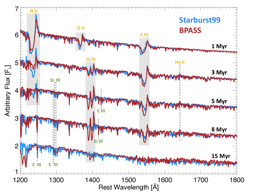
Star light between 1200-2000Å is dominated by young, massive O-stars. Consequently, we used fully theoretical stellar models with young ages corresponding to 1, 2, 3, 4, 5, 8, 10, 15, 20 and 40 Myr. At 1270Å, a 20 Myr stellar population of a given initial mass is nearly two orders of magnitude fainter than a 1 Myr stellar population, while older populations are fainter still (Leitherer et al., 1999; Eldridge et al., 2017). Moreover, the UV stellar continua of older stellar populations evolve more slowly with time, such that there are small spectral differences between a 50 and 100 Myr stellar population (fig. 5 in de Mello et al., 2000). Finally, the effective temperature of B-star populations greater than 40 Myr drops below the 20,000 K threshold where high-resolution stellar templates are computed using the WM-Basic code (Leitherer et al., 2010). Thus, the selected age range includes models of the most luminous O-stars whose spectral features vary rapidly with time at sufficient spectral resolution to resolve these important spectral features.
We use the five Z∗ models that are available from the Geneva stellar atmospheres (Meynet et al., 1994): 0.05, 0.2, 0.4, 1.0, and 2.0 Z⊙. Combined, each observed spectrum is fit with 50 fully theoretical stellar models and one free parameter for the dust attenuation, for a total of 51 total free parameters.
Other stellar physics impact the production of ionizing photons, such as rapid rotation (Levesque et al., 2012; Leitherer et al., 2014; Choi et al., 2017) and a varying (or stochastically populated) IMF (Leitherer et al., 1995; Rigby & Rieke, 2004; Crowther, 2007). However, the stellar population synthesis routines only include two Z∗ (0.14 Z⊙ and 1 Z⊙, but see the recent extension to 0.02 Z⊙ from Groh et al., 2019), which samples metallicity too coarsely for our fitting. Consequently, binary models are the only alternative stellar model that we discuss below.
3.2.1 The fiducial case: starburst99 single-star models
We used the fully theoretical starburst99 models with Geneva atmospheres that incorporate high-mass loss rates (Meynet et al., 1994) as our fiducial model. These models have a spectral resolution of 0.4Å, which match the spectral resolution of the MegaSaura spectra. We convolved the models with a Gaussian to match the observed spectral resolution of each individual MegaSaura spectrum, as measured from the optical sky emission lines (Rigby et al., 2018a), and resampled the stellar models onto the wavelength grid of the observations. Similarly, we convolved the higher resolution HST/COS data to the 0.4Å spectral resolution of the starburst99 models from the spectral resolution measured from the Milky Way absorption lines (Chisholm et al., 2016). Each model spectrum was normalized to the median flux density between 1267–1276Å.
The starburst99 stellar models were created using the WM-Basic method (Pauldrach et al., 2001) and densely sample the high-mass portion of the Hertzsprung-Russell diagram up to temperatures of 20,000 K. WM-Basic does not calculate high-resolution models below these temperatures (Leitherer et al., 2010). Consequently, we chose the ten stellar ages between 1–40 Myr listed above with stellar temperatures greater than 20,000 K. These models include Wolf-Rayet (WR) stars using the Potsdam Wolf-Rayet code (PoWR; Sander et al., 2015), but the evolutionary tracks predict that few if any WR stars are present in low-metallicity stellar population, such that the WR spectra are rarely incorporated into 0.2–0.4 Z⊙ starburst99 models (Leitherer et al., 2018).
3.2.2 The binary evolution case: bpass models
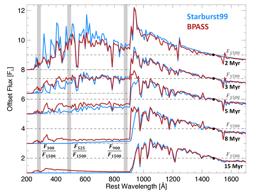
We also used the Binary Population and Spectral Synthesis (bpass) v2.2.1 models222https://flexiblelearning.auckland.ac.nz/bpass/9.html, which include binary star evolution (Stanway & Eldridge, 2018b). bpass models have a larger metallicity range, but, for consistency, we used the same five Z∗ available from the Geneva models. bpass models use a custom set of O-star models created with WM-Basic at 1Å resolution for O-stars with temperatures greater than 25,000 K (Eldridge et al., 2017). Temperatures less than this have the baselv3.1 and C3K models which have spectral resolution of 20Å below 1500Å (Westera et al., 2002; Le Borgne et al., 2003; Conroy & van Dokkum, 2012; Conroy et al., 2014). Therefore, bpass models are lower resolution when ages are greater than 20 Myr for any metallicity and when ages are greater than 15 Myr for metallicities greater than 0.4 Z⊙ (see Figure 1). This spectral resolution is too low to diagnose many of the narrow B-star features of older stellar populations and cannot be used to distinguish older stellar populations. For this reason, we chose the starburst99 models as our fiducial model. We return to this issue in Section 5.4.2.
3.3 The nebular continuum
Young massive stars produce large amounts of ionizing photons which produce free-free, free-bound, and two-photon nebular continuum emission. The nebular continuum heavily contributes to the total continuum flux at young ages, low metallicities, and redder wavelengths (Steidel et al., 2016; Byler et al., 2018). For a stellar continuum metallicity of 0.05 Z⊙ and a stellar age of 1 Myr, the nebular continuum is 25% of the stellar continuum at 2000Å.
We created a nebular continuum for each age, metallicity, and stellar model by processing the stellar continuum models through cloudy v17.0 (Ferland et al., 2013). We assumed that the gas-phase metallicity and stellar metallicity were the same (Section 5.1), an ionization parameter of log(U) , and cm-3. We produced a nebular continuum for each stellar population, added the output nebular continua to the stellar models, and normalized by the flux between 1267–1276Å. The inclusion of the nebular continuum produces redder stellar models than before, which has a pronounced impact on the fitted E(B-V) of young stellar populations.
We tested the effect that different ionization parameters have on the fitted stellar ages and metallicities by also creating models with log(U) , 2.3, 2.7, and 3.0. We found that the reduced of the resultant fits do not change statistically for the different log(U) values. Consequently, we adopted a midrange log(U) = 2.5 for all galaxies.
3.4 Stellar population parameters derived from the fits
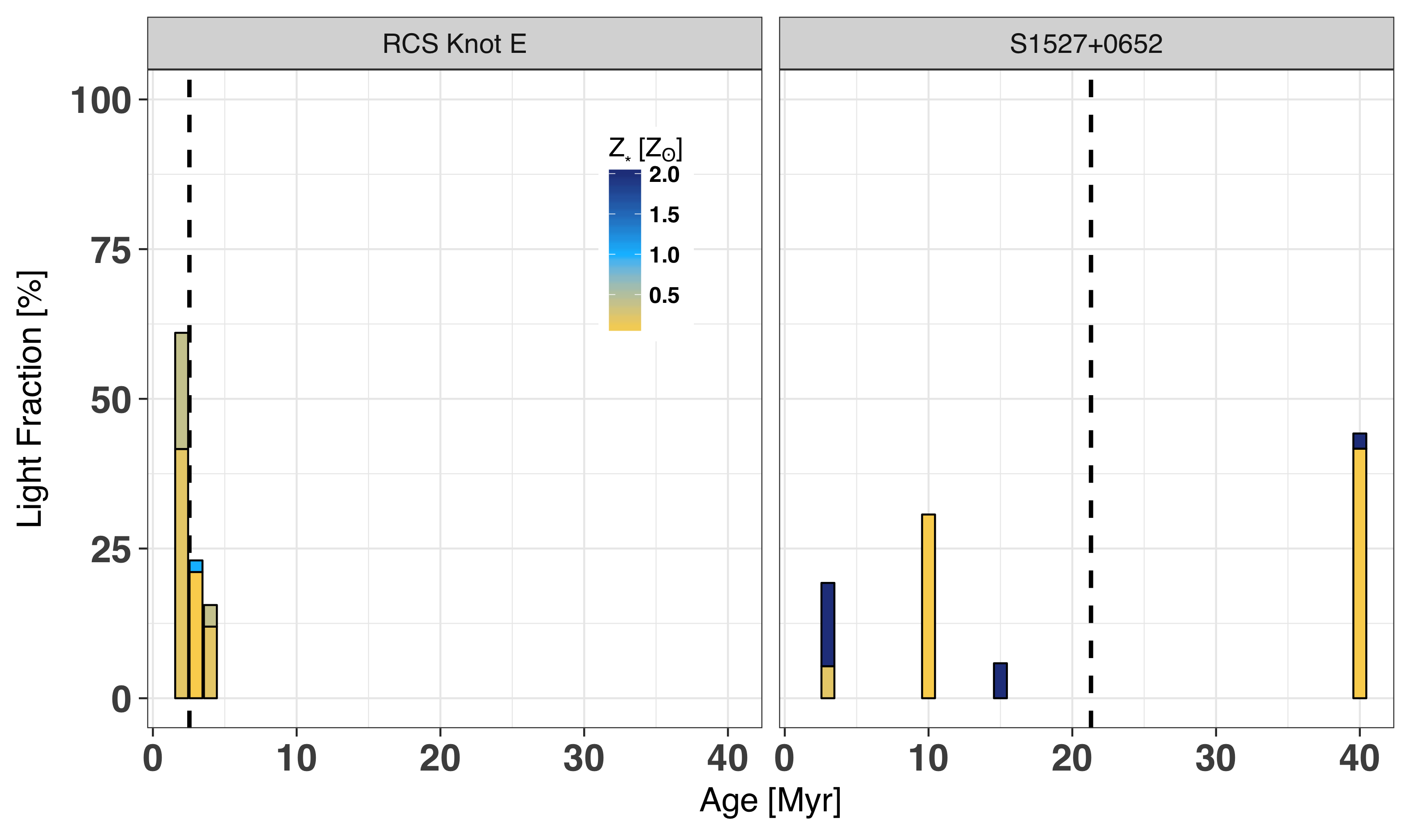
The observed stellar continua are fit by statistically determining the linear multiplicative coefficient, , for the 50 single age, single metallicity stellar models (; Equation 1). These linear coefficients can take any value greater than or equal to 0 and MPFIT determines the linear combination that best fits the observed stellar continuum. In practice, the code typically assigns values to most of the stellar models, and only gives power to a small subset of the models (on average 6 models have light fractions ¿0%). Figure 2 shows the distribution of the light at a given age for two observed stellar populations fitted with the multiple population method. All of the light from RCS Knot E comes from a very young, moderate metallicity stellar population (left panel); while the stellar light from S1527+0652 is broadly distributed across age and metallicity (right panel).
We determined intrinsic stellar parameters from the fitted coefficients in Equation 1. The derived parameters are a weighted average of the total light at 1270Å attributed to the individual stellar models (). Thus, each property derived below is a “light weighted” property. First, the light fraction () that each model contributes to the total intrinsic flux at 1270Å is defined as:
| (2) |
Secondly, the light-weighted age at 1270Å is defined as:
| (3) |
The light-weighted ages of RCS Knot E and S1527+0652 are indicated as vertical lines in the left panel of Figure 2. Finally, we computed the light-weighted stellar metallicity as:
| (4) |
These three parameters describe the properties of the observed stellar populations. The uncertainties on these parameters were derived by varying the observed flux density at every wavelength by a random Gaussian kernel with width equal to the flux uncertainty at that wavelength. We then recalculated the ages and Z∗, tabulated each value, and repeated the procedure 100 times. The standard deviation of each age and Z∗ distribution is the uncertainty on the age and Z∗, respectively. We include the , Z∗, and light-weighted ages in the electronic version of the Appendix.
All of these stellar population properties (age and metallicity) are light-weighted at 1270Å; they cannot be directly compared to similar properties derived at other wavelengths. Younger stars produce relatively more light at bluer wavelengths than older stars, biasing the light from young stars to bluer wavelengths. The ages derived from full SED modeling using optical and near-infrared observations will inherently return older ages than we estimated because optical light comes from older stars.
An important measure of the ionizing continuum is the ratio of the intrinsic flux density at 900Å to the flux density at 1500Å (F900/F1500). Observations compare the observed F900/F1500 to the intrinsic F900/F1500 to determine the fraction of ionizing photons that escape galaxies (Steidel et al., 2001). We estimate the intrinsic F900/F1500 by extending the stellar population fits to bluer wavelengths than the observations and removing the contributions from dust attenuation (setting E(B-V) = 0 in Equation 1). The high-resolution starburst99 models are only defined at Å, consequently, we created low-resolution starburst99 models (20Å resolution; Leitherer et al., 1999) using the same model parameters and fitted light-fractions as the high-resolution models. We then measured the median model flux density between 895–906Å, for F900, and 1495–1506Å, for F1500.
Ionizing photons with higher energies create high-ionization gas (e.g. O++). We also inferred the stellar flux density between 510–540Å (F525) and between 280–320Å (F300) to determine how many high-energy photons a given stellar populations produces. F525 (with photon energies of 24 eV) probes photons that singly ionize oxygen, but do not ionize helium. Meanwhile, F300 (photon energies of 41 eV) probes photons that doubly ionize oxygen and singly ionize helium, but do not doubly ionize helium. These wavelengths were carefully chosen to probe the peak of the stellar SEDs, while avoiding contributions from strong stellar absorption and emission features (see Figure 1).
Finally, all derived parameters are either flux density ratios (e.g., F900/F1500) or derived from normalized spectra (e.g., stellar age). This means that the stellar population parameters are independent of the intrinsic luminosity, which depends on the magnification from gravitational lensing.
4 Relating spectral features and inferred stellar population properties
| Line | bpass Age | starburst99 Age |
|---|---|---|
| [Myr] | [Myr] | |
| Stellar wind lines | ||
| N V 1240Å | 15 | 110 |
| O V 1371Å | 12 | 14 |
| Si IV 1400Å | 315 | 35 |
| C IV 1550Å | 115 | 110 |
| He II 1640Å | 420 | 34 |
| Photospheric lines | ||
| C III 1247.4Å | 415 | 540 |
| Si III 1294.5Å | – | 540 |
| C III 1296.3Å | – | – |
| Si III 1296.7Å | – | 540 |
| Si III 1298.9Å | – | 540 |
| Fe V 13461365Å | 115 | 120 |
| Fe V 14271430Å | 115 | 120 |
| S V 1501.8Å | 18 | 140 |
| Fe IV 15261534Å | 310 | 340 |
| Si II 1533Å | – | 840 |
| Fe III 19231966Å | 1040 | 1040 |
Often times the ages of stellar populations are deduced using the broadband UV through IR SED shapes. While the SED shape provides important age information, it is often degenerate with metallicity and dust attenuation. By contrast, fitting the stellar spectral features with theoretical stellar templates simultaneously determines the age, metallicity, and dust attenuation of the stellar populations. Consequently, the light-weighted ages and metallicities derived above are driven by spectral features which are less degenerate than the spectral shape alone (see Figure 1 and Table 1).
The two main types of FUV stellar features are strong, broad stellar wind P-Cygni features and weak stellar photospheric absorption lines. Both types of features can be contaminated by neighboring ISM absorption, and require high SNR and moderate spectral resolutions to resolve. In the following two subsections, we discuss both types of spectral features individually, and illustrate how the individual features relate to the inferred stellar population ages and metallicities. The purpose of these subsections is not to advocate for determining the stellar ages and metallicities using single features, but rather to demonstrate that the stellar properties inferred from the full spectral fits are entirely consistent with the trends of stellar spectral features.
4.1 Stellar wind features
The most notable stellar features in the FUV are the broad blueshifted absorption and redshifted emission profiles (called P-Cygni profiles; orange labels in Figure 1). These P-Cygni profiles arise from strong winds that are radiatively driven off of stellar photospheres (Castor et al., 1975; Lamers & Cassinelli, 1999). The terminal velocity, ionization structure, and mass-outflow rates sensitively depend on the stellar luminosity (Castor et al., 1975; Lamers & Leitherer, 1993; Lamers et al., 1995; Leitherer et al., 1995; Puls et al., 1996; Kudritzki & Puls, 2000). The terminal velocity describes the maximal velocity extent of the absorption component, while the mass-loss rate determines the depth of the profile. In turn, these establish the shape of the P-Cygni absorption and emission.
Whether a given ion is observed as a P-Cygni profile in the wind depends on the ionization structure of the stellar wind. The peak ionization stages for stellar winds typically are the C V, N IV, O IV, and Si V states (Lamers & Cassinelli, 1999), none of which have resonant transitions in the rest-frame FUV. Alternatively, the presence of adjacent ionization stages with P-Cygni profiles (N V, C IV, or Si IV) provides information on the stellar temperature of the most luminous stars and, by inference, the stellar population age. The age of a stellar population can be inferred from the strength of the observed P-Cygni transitions: O V and N V have the highest ionization states and are strongest in stars with lifetimes of 2-3 Myr, while C IV and Si IV are lower ionization and peak in stars with lifetimes near 5 Myr.
Stellar temperature, or age, is not the sole determinant of the stellar wind profiles. Metals in the photospheres of hot stars absorb continuum photons which is what accelerates the gas off the stellar surface. Consequently, the stellar metallicity determines both the acceleration and mass outflow rate of the stellar wind (Lamers & Cassinelli, 1999; Vink et al., 2001). The terminal velocities and mass-loss rates of O-stars with Z⊙ have been empirically determined to scale as Z and Z, respectively, (Leitherer et al., 1992; Vink et al., 2001). Lower metallicity stellar winds of resolved individual stars have not been observed, consequentially the mass outflow rate and terminal velocity relations have been extrapolated to lower metallicities. These relations illustrate how stellar wind P-Cygni absorption profiles scale with stellar metallicity.
In the next five sub-sections we walk through the individual P-Cygni lines in the FUV. Each subsection explores the theoretical and observed wind features and their relationship to the inferred stellar population age and metallicity. In Section 4.3 we conclude that the N V P-Cygni and He II emission are strong in very young stellar populations, while the shape of the C IV P-Cygni profile changes both with stellar age and metallicity (see Figure 3). Conversely, the Si IV of our sample is dominated by interstellar absorption, and the O V line is not observed. Collectively, the stellar wind profiles mimic the inferred stellar ages and metallicities.
4.1.1 The C IV P-Cygni feature
The C IV feature is strong, broad, and has a P-Cygni profile for all of the MegaSaura galaxies (there is not C IV coverage for many of the low-redshift COS spectra). Further, the C IV P-Cygni profile is sufficiently broad that stellar and interstellar components can easily be separated with moderate spectral resolution (see shaded regions in Figure 4 and Figure 5). The C IV profile probes stellar outflows from 1-10 Myr populations and the absorption component distinctly varies with Z∗ (Figure 3). This makes it an ideal diagnostic of stellar age and metallicity.
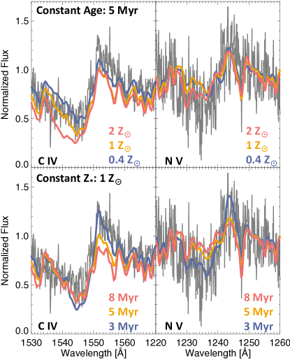
Different portions of the C IV profile depend on either Z∗ or stellar age (left panels of Figure 3). At a constant 5 Myr age (upper left panel), the C IV absorption of the starburst99 models deepen and broaden as Z∗ increases from 0.4 Z⊙ (blue line) to 1 Z⊙ (gold line) to 2 Z⊙ (pink line), because the C IV mass-loss rate strongly increases with Z∗. Conversely, the models predict that the C IV emission is nearly independent of Z∗. Meanwhile, at a constant 1 Z⊙ metallicity (lower left panel), the modeled C IV absorption is independent of stellar age, but the emission strongly peaks at ages ¡5 Myr (blue line). In summary, the C IV absorption varies with Z∗ and the C IV emission varies with stellar age.
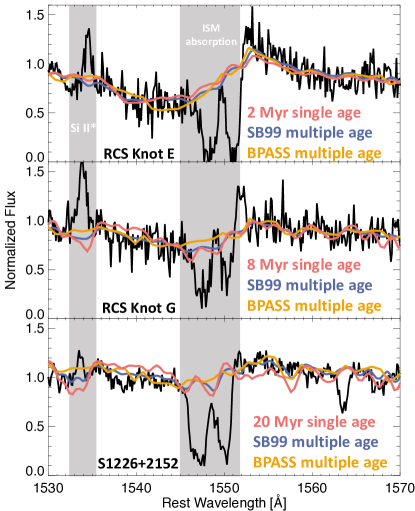
The temporal evolution of C IV found in the models is clearly corroborated by the light-weighted ages. Figure 4 shows three MegaSaura spectra ordered in descending light-weighted stellar age and each have similar light-weighted metallicities ( Z⊙). Overplotted in red is a single age starburst99 model with a population age nearest to the inferred light-weighted age. The C IV emission is strongest in the youngest populations and adequately matches the triangular wind emission from the RCS Knot E spectrum. Meanwhile, RCS Knot G, a different region from the same galaxy, has weaker P-Cygni emission (although note the narrow nebular C IV emission), similar to an 8 Myr single age population. Finally, S1226+2152 has an even older inferred light-weighted age; the C IV P-Cygni feature has nearly disappeared and has been replaced by a flat C IV feature with narrow, interstellar absorption. The derived light-weighted ages of each spectrum are consistent with the by-eye P-Cygni variation: Knot E, Knot G, and S1226+2152 have starburst99 light-weighted ages of 2.5, 11, and 26 Myr, respectively.
While the single age models reflect the C IV profiles of the youngest populations, they do not describe all of the galaxy-to-galaxy P-Cygni variations in the older populations. The C IV absorption from RCS Knot G is deeper at bluer velocities than the 8 Myr single age model, while S1226+2152 has a small amount of redshifted emission. The observed stellar populations are not single age populations, but the multiple age fits capture the different populations (blue and gold lines in Figure 4 are the starburst99 and bpass fits). While a single age population largely describes the C IV emission from the youngest populations, older populations require a mix of both young and old stars to match the observations.
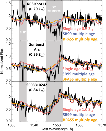
Metallicity has a similarly strong impact on the shape of the observed C IV profile, but this time on the absorption portion of the P-Cygni profile. The upper left panel of Figure 3 shows that Z∗ mostly impacts the depth and width of the absorption component. This is further illustrated in Figure 5 which shows three MegaSaura spectra with nearly constant stellar age (5, 3, and 5 Myr) but with increasing stellar metallicity. At 0.3 Z⊙ (top panel), the C IV absorption only reaches a depth of 0.6 in normalized flux units. Increasing the metallicity to 0.6 Z⊙ (middle panel) creates a pronounced, broad P-Cygni absorption profile that reaches 0.5 in normalized flux units. Finally, by 0.8 Z⊙ (bottom panel) the stellar wind dominates the C IV spectral region and the absorption reaches 0.4 in normalized flux units. The stellar emission does not strongly change with Z∗, as the stellar emission peaks near for all of these spectra. Both the stellar models and the observed spectra indicate that the stellar metallicity strongly shapes the absorption component of the C IV P-Cygni profile.
To summarize: the C IV profile strongly varies with the inferred light-weighted stellar population properties. The C IV P-Cygni absorption depends on the Z∗ and the emission depends on the stellar age (Figure 3). The multiple age and multiple metallicity fits to the C IV P-Cygni profiles mimic changes in the inferred stellar age (Figure 4) and metallicity (Figure 5).
4.1.2 The N V P-Cygni feature
The N V 1240Å stellar wind profile largely depends only on stellar age. The age dependence arises because the dominant ionization state of an O-star wind is N+++, but as the stellar temperature increases with decreasing Z∗, N+++ gas is heated into the N4+ state. This heating produces relatively more gas in the N4+ ionization state for low Z∗ winds than higher Z∗ winds and nearly balances the decreasing metallicity (Kudritzki, 1998; Lamers & Cassinelli, 1999; Leitherer et al., 2010). The models in the upper right panel of Figure 3 show the negligible N V variation with Z∗, while strong absorption and emission only occurs at ages young enough to produce N V stellar winds (bottom right panel of Figure 3). N V only arises from very young (¡5 Myr) stellar populations.
A strong N V profile is detected in most FUV spectra in Figure 6. The exceptions are the oldest stellar populations which do not show P-Cygni profiles in either the C IV or the N V ionization state (e.g. S1527+0652). Weak C IV and a non-detection of N V indicates that there is not currently a young (¡8 Myr) stellar population in these older galaxies (see the discussion in Section 5.3). In contrast, the normalized flux of the N V profile from the Sunburst Arc varies by a factor of 2.5 from the absorption depth to the emission peak, illustrating the strong N V P-Cygni profiles in populations with very young light-weighted ages. This trough-to-peak ratio decreases with increasing inferred stellar population age in Figure 6: it is 2.2 for S0033+0242 with an age of 5 Myr and 1.4 for S1429-1202 with an age of 15 Myr.
4.1.3 The Si IV P-Cygni feature
P-Cygni Si IV is generally observed in supergiants (evolved stars) or in metal-rich stars because the dominant ionization state in main-sequence stellar winds is the Si4+ state. Thus, the Si+++ ionization state is too low of a temperature to trace the bulk of the O-star wind (the opposite behavior as N V above; Walborn & Panek, 1984). As O-stars evolve into supergiants, their stellar photospheres expand and the stellar winds become denser, causing the dominant ionization state, Si4+, to recombine into Si+++. These denser winds produce prominent Si IV P-Cygni features in the spectra of evolved O-stars (Drew, 1989; Pauldrach et al., 1990). Similarly, the ionization structure also shifts towards lower ionization stages as larger stellar metallicities produce relatively more Si+++ in their stellar winds. Thus, the stellar models predict that Si IV P-Cygni profiles are only strong in stellar populations with a lower ionization structure, either from higher metallicity stars or an out-sized contribution of evolved stars.
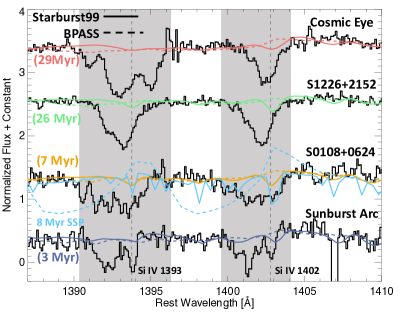
Strong Si IV 1400Å ISM absorption is seen in Figure 7, but Si IV is rarely observed to have a stellar P-Cygni profile. The entirety of the observed Si IV absorption can be explained by narrow interstellar absorption that reaches nearly zero flux. After accounting for interstellar absorption (gray regions in Figure 7), the observed Si IV region is nearly featureless. The lack of strong P-Cygni Si IV suggests that the stellar populations within our sample are either metal poor (see Section 5.1) or not dominated by evolved stars. We conclude that the observed Si IV regions are dominated by interstellar absorption and that Si IV does not strongly vary with the stellar population properties.
4.1.4 The He II emission feature
He II 1640Å stellar emission arises from extremely hot evolved Wolf-Rayet stars. Wolf-Rayet stars are a short-lived supergiant phase associated with stars that have main-sequence lifetimes less than 5 Myr (Abbott & Conti, 1987; Crowther, 2007). Wolf-Rayet stars have broad He II emission lines in both the optical and FUV that are strongest in higher metallicity stars (Schaerer & Vacca, 1998).
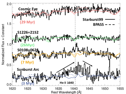
He II in Figure 8 is not observed as a broad P-Cygni profile like N V or C IV. For the oldest light-weighted populations, He II is a weak absorption line (equivalent width of Å in S1226+2152). Conversely, the youngest populations (Sunburst Arc, RCS Knot E, S0033+0242, and RCS Knot U) have a broad triangular shaped He II emission profile (see the arrows in Figure 8). The He II emission resembles the redshifted triangular C IV emission profile but without the blueshifted absorption component that creates the P-Cygni profile. There is not He II absorption because He II 1640Å is not a resonant transition (it is analogous to H), therefore the stellar wind is optically thin to the He II recombination emission. The He II emission equivalent width from the Sunburst Arc spectrum is 1.2Å and it has a FWHM = 379 km s-1, consistent with a 3 Myr, 0.5 Z⊙ Wolf-Rayet model (Schaerer & Vacca, 1998). The presence of a broad He II emission profile strongly suggests that the spectrum is dominated by a Myr stellar population.
Finally, S0108+0624 is the only galaxy in the sample with statistically significant (), narrow He II emission (equivalent width of Å and FWHM = 96 km s-1, which is resolved by the 69 km s-1 spectral resolution). This narrow emission appears nebular in origin when compared to the broad Wolf-Rayet feature of the Sunburst Arc (compare the bottom and second-to-bottom spectra in Figure 8). This He II emission is at the weak end of the range of He II equivalent widths seen in local dwarf galaxies ( to Å; Berg et al., 2016, 2019). We return to possible origins of the nebular He II emission in Section 5.4.4.
The multiple age fits to the He II region are fairly poor. This is especially true for galaxies with strong WR emission (e.g. the Sunburst Arc). The bpass models fit the He II region substantially better than the starburst99 models do, although they still do not match the WR features of younger populations. While both stellar models include WR models, neither model appears to produce a sufficient number of WR stars to match the broad He II emission observed in the youngest stellar populations (e.g., Leitherer et al., 2018).
Overall, we find broad Wolf-Rayet He II emission in stellar populations with the youngest light-weighted ages and weak He II absorption in older populations.
4.1.5 The O V wind feature
With an ionization potential of 117 eV, O V 1371Å is the highest ionization line between 1200-2000Å and traces the hottest outflowing phase from the most massive stars (up to 106 K). This feature is an unambiguous indicator of the youngest stars and disappears once the stellar population ages past 3 Myr (see Figure 1 and Table 1).
While O V is an ideal tracer of the most massive stars, it is not strongly observed in any of the MegaSaura or COS spectra. This may indicate that there is not a significant extremely massive stellar population (300 M⊙), but more likely it indicates that the winds of the most massive stars are significantly clumpier–thus denser–than assumed in the model atmospheres. Denser, clumpier winds lead to lower ionization stellar winds and reduced O V profiles (Bouret et al., 2003; Leitherer et al., 2010).
4.2 Photospheric absorption lines
The broad, pronounced stellar wind features, fully discussed in the previous section, arise as intense radiation fields accelerate gas off of stellar surfaces. However, gas within the stellar photospheres also absorbs stellar radiation. These photospheric absorption lines are narrower and weaker than the stellar wind lines because the photosphere is relatively static, but provide similarly robust indicators of stellar age and Z∗ (de Mello et al., 2000). Since photospheric gas is denser than interstellar gas, photospheric lines typically arise from excited states that are easily separated from ISM lines.
High-ionization photospheric lines, like S V 1502Å, are found in the spectra of young stars, but the rest-frame FUV has a host of O-star diagnostics, such as stellar wind lines, that are stronger features and diagnose the stellar population properties at a lower SNR. The photospheric lines excel in diagnosing older (¿7Myr), B-star dominated populations (de Mello et al., 2000), because the photospheric features are the only distinguishing features of B-stars in the FUV continuum. Previous authors have suggested that individual lines (see Table 1; de Mello et al., 2000) and bands of photospheric lines near 1417Å and 1935-2020Å identify B-star populations (Rix et al., 2004).
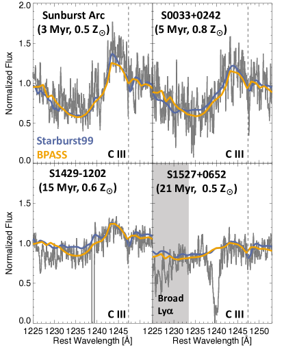
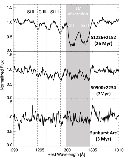
Our moderate-resolution data reveal that the C III and Si III photospheric lines at 1247Å (see Figure 6) and between 1295–1299Å (specifically C III 1299Å; see Figure 9) are the strongest due to their low excitation energies (6 eV versus 10-30 eV for the features near 1420Å; Leitherer et al., 2011). The 1290Å lines blend with neighboring O I and Si II ISM absorption features at low spectral resolution, however, at moderate resolution the Si III 1299Å line is resolved. Figure 3 clearly shows that Si III strengthens in stellar populations older than 5-10 Myr. The Si III 1299Å equivalent width decreases from Å for S1226+2152 with an age of 26 Myr, to for S0900+2234 with an age of 7 Myr, to undetected (Å) for the Sunburst Arc at 3 Myr. Similarly, the other three MegaSaura galaxies with ages less than 6 Myr (RCS Knot E with an age of 2 Myr, S0033+0242 with an age of 5 Myr, and RCS Knot U with an age of 5 Myr) have undetected Si III 1299Å (equivalent widths of , , and Å, respectively). Very young populations do not contain the C III 1299Å photospheric feature.
There are multiple Fe photospheric lines in the FUV that arise from the Fe III, Fe IV, and Fe V ionization states (Table 1; Nemry et al., 1991; de Mello et al., 2000; Rix et al., 2004). These Fe lines (specifically Fe V in O-stars) blanket the spectral regions, overlap in wavelength, and form large-scale continuum features that change the shape of the stellar continuum. These Fe features are included in the full spectral fitting, however, even at the high SNRs of the MegaSaura sample, the Fe lines are very weak.
The power and utility of the stellar photospheric lines is limited because the photospheric lines are significantly weaker than the stellar wind features, requiring extremely high SNR observations. At the SNR and spectral resolution of our observations, the most prominent photospheric lines are near 1299Å and these features indicate the presence of stars with ages 7 Myr.
4.3 Summary: Individual spectral features are consistent with inferred stellar ages and metallicities
| Region | Spectral Feature within Region | Age | Z⊙ |
|---|---|---|---|
| 1225-1250 | N V | 7.3 | 1.4 |
| 1250-1350 | Si III 1299Å | 2.4 | 2.1 |
| 1380-1410 | Si IV | 0.8 | 1.7 |
| 1420-1520 | Featureless | 2.0 | 2.4 |
| 1530-1560 | C IV | 2.6 | 3.1 |
| 1660-1760 | Featureless | 1.3 | 1.7 |
| 1900-2000 | Featureless | 1.6 | 1.0 |
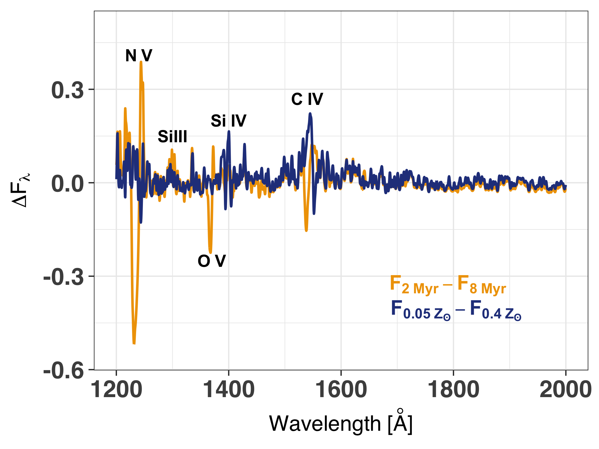
Throughout this section we have compared the light-weighted stellar population properties (age and metallicity) to individual stellar features, but in all cases the inferred stellar properties were determined from the entire observed wavelength regime. In Figure 10 we plotted the change in flux density () that occurs due to varying the stellar age (gold) or metallicity (blue). The largest arises from the strong stellar wind and photospheric lines that we emphasized above. We demonstrated this by integrating the within specific wavelength regions to determine the total flux change attributable to individual spectral regions (Table 2). The N V profile changes almost exclusively with age and is weakly dependent on Z∗. Similarly, the Si IV region largely depends on Z∗ and hardly depends on stellar age (compare Column 3 and 4 in Table 2). While the notable stellar wind features dominate Figure 10, small spectral features occur outside these regions that on aggregate differentiate between stellar properties. For instance, the region between 1420–1520Å is devoid of prominent stellar wind features, but the shape of the stellar continuum noticeably changes over 100Å due to the stellar population age and Z∗. The 1420–1520Å region changes the flux comparably to the broad C IV P-Cygni wind feature and the Si III 1299Å photospheric regions, and has more power to differentiate stellar properties than the Si IV wind region. This implies that ”featureless” regions of stellar continuum hold significant power to determine stellar age and Z∗. The power in these regions stems from the fact that they are not featureless, but crucially contain weak photospheric metal features like Fe III, Fe IV, and Fe V (Nemry et al., 1991; de Mello et al., 2000; Rix et al., 2004). In other words, the previous sections were not advocating to use a single feature to determine the stellar properties, rather the sections illustrated that the spectral features consistently and distinctly vary according to the inferred stellar population properties from the full stellar continuum.
Young stellar populations produce the most ionizing photons. Thus, it is important to have spectral features that distinguish immense sources of ionizing photons. There are spectral indices that are unique to very young (¡7 Myr) stellar populations: (1) strong and broad C IV and N V P-Cygni features (Figure 3), (2) broad (¿300 km s-1) He II emission (Figure 8), and (3) undetected Si III 1299Å photospheric absorption features (equivalent widths ¡0.1Å; Figure 9). These spectral signatures suggest that the stellar population is dominated by stars younger than 7 Myr. Older stellar populations appear to have combinations of both young and old stars, obscuring single trends in spectral features (see Section 5.3).
5 Discussion
5.1 Nebular gas and massive stars have similar metallicities
The stellar metallicity is a fundamental galaxy property that is traditionally challenging to measure, but crucially determines the production of ionizing photons. Previous observations have either used spectral indices (e.g., Rix et al., 2004; Leitherer et al., 2011; Byler et al., 2018) or full spectral synthesis (e.g., Pettini et al., 2000; Kudritzki et al., 2012; Steidel et al., 2016; Steidel et al., 2018; Hernandez et al., 2019) to estimate the metallicities of young stellar populations. Here, we explore the relation between the light-weighted Z∗ derived from the full spectral synthesis to the observed gas-phase metallicities derived from rest-frame optical nebular emission lines (Zneb).
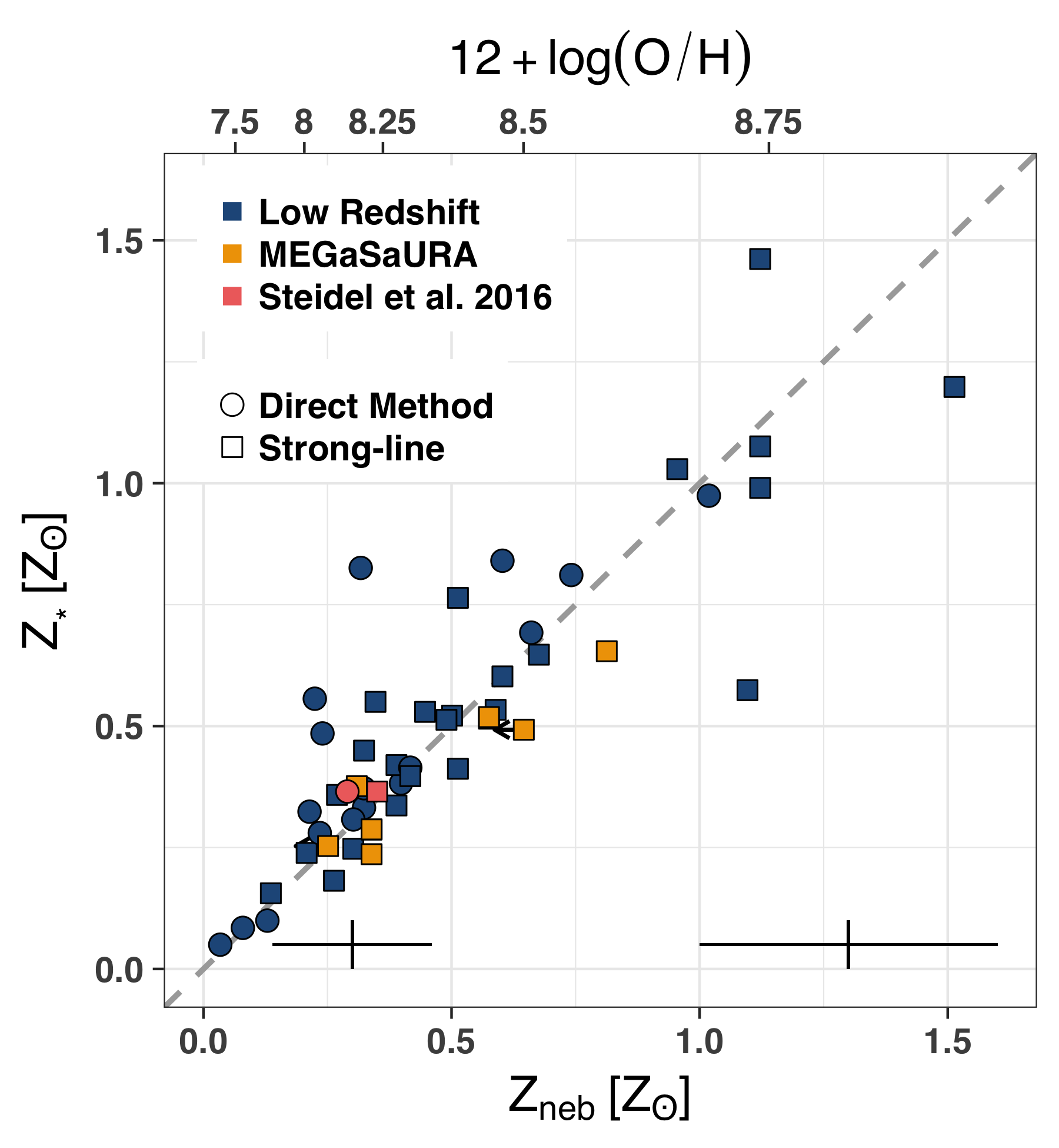
Figure 11 shows that the light-weighted Z∗ and the Zneb are correlated at the significance (with a Pearson’s correlation coefficient of 0.87). The metallicities scatter about the one-to-one line, indicating that the young massive stars have a similar metallicity as the surrounding nebular gas. Both the low and high-redshift galaxies are near the one-to-one line; this relationship does not appear to evolve with redshift. There is a dearth of points above 1 Z⊙, largely as a selection effect of both samples. While we have used direct metallicities whenever possible (see the discussion in Section 2.3), we have used different metallicity calibrations which can have a 0.4 dex scatter in their relative metallicity calibrations. The largest outlier from a one-to-one relationship is NGC 3256, in the lower right quadrant with Z∗ = Z⊙ and Zneb = Z⊙ (including calibration uncertainties; Engelbracht et al., 2008). Consequently, the Zneb of the largest outlier is still consistent with Z∗ at the 1.3 significance level.
Further, we measure the residual standard error of the trend to be 0.16 Z⊙, or 0.17 dex in 12+log(O/H) at the median Zneb of 0.4 Z⊙. This residual standard error is consistent with the full 0.4 dex spread found by Kewley & Ellison (2008) between the Pettini & Pagel (2004) and Kobulnicky & Kewley (2004) metallicity calibrations (the two most commonly used strong-line methods here). Thus, the observed dispersion in Figure 11 is entirely consistent with the spread of the different 12+log(O/H) calibration methods.
Z∗ is surprisingly consistent for the lowest metallicity populations. The stellar mass-loss rate, and in turn the stellar wind profile, is only empirically constrained for Z∗ ¿ 0.2 Z⊙ and the 0.05 Z⊙ starburst99 models instead rely on an extrapolation of the mass-loss rates to lower metallicities (Leitherer et al., 1992; Vink et al., 2001). The close metallicity correspondence below 0.2 Z⊙ suggests that the stellar wind extrapolation adequately reproduces the observed stellar wind profiles and their mass-loss rates. Zneb for 1 Zw 18 is lower than 0.05 Z⊙, the lowest Meynet et al. (1994) atmospheric model, leading to a possible over-estimate of the light-weighted Z∗ for this galaxy.
The strong relationship between Zneb and Z∗ in Figure 11 suggests that Z∗ robustly determines the metallicities of galaxies. A robust metallicity indicator is need at high-redshifts as the crucial, yet extremely faint, metallicity sensitive lines, like [O III] 4363Å, are redshifted out of the optical (Yuan & Kewley, 2009; James et al., 2014a; Sanders et al., 2016). Recent work has attempted to calibrate Zneb using rest-frame UV emission lines (Pérez-Montero & Amorín, 2017; Byler et al., 2018), but these calibrations depend on rather uncertain assumptions of the carbon-to-oxygen abundance that are not yet well calibrated. Fortunately, Figure 11 implies that observations from the ground using upcoming large telescopes and the rest-frame FUV stellar continuum may constrain the chemical enrichment of galaxies to redshifts of .
The similarity of Zneb and Z∗ indicates that the gas surrounding high-mass stars is not instantaneously metal-enriched by massive stars. In other words, it takes longer than the inferred lifetimes of the massive star populations to increase the metallicity of adjacent ISM gas. Newly synthesized metals are ejected from star-forming galaxies as very hot supernovae ejecta and galaxies must take longer than the 107 yr timescales observed here to fully mix these newly synthesized metals (Kobulnicky & Skillman, 1997). In fact, we did not find a statistical correlation between Zneb and the stellar age, implying that gaseous enrichment either occurs on longer timescales than observed here, or that the enrichment of a single stellar population is within the scatter of Figure 11.
5.2 The ionizing continua of massive stars
The non-ionizing FUV continua of massive stars are rich with features that diagnose the stellar population age and metallicity. The primary goal of this paper is to use these inferred light-weighted metallicities and ages to constrain the ionizing continua of massive stars. The same massive stars that produce the FUV spectral features also produce the unseen ionizing continua; these spectral features are the most direct probe of the ionizing continua because they only depend on the massive star properties (unlike nebular emission lines which also depend on the gaseous properties). We therefore use the theoretical stellar models to develop simple prescriptions for how the ionizing continuum varies with stellar properties (Section 5.2.1) and then infer the ionizing continua from the FUV observations using the stellar fits (Section 5.2.2). We refer to the ionizing continua determined from the models as the inferred ionizing continua to emphasize that we do not directly observe the ionizing continua. Throughout this sub-section we only focus on the starburst99 fits; we return to the bpass fits in Section 5.4.
5.2.1 Stellar population properties determine the ionizing continua of massive stars
The full ionizing continuum will likely never be observed because foreground neutral hydrogen efficiently absorbs these photons. Observations are typically fortunate to observe the ionizing continuum at a single wavelength, which is most feasible at 900Å. This ionizing flux density is then normalized by the observed non-ionizing continuum to control for stellar mass and star formation contributions. Thus, the literature typically quantifies the ionizing continuum through the ratio of the flux at 900Å (ionizing) to the flux at 1500Å (non-ionizing), or F900/F1500 (Steidel et al., 2001). In this subsection, we use the starburst99 fully theoretical models to explore how the stellar properties determine this ratio as well as flux density ratios at other ionizing to non-ionizing wavelengths.
Figure 12 shows the theoretical ionizing continua of single burst, 0.4 Z⊙, starburst99 stellar populations at five different ages. At 2 Myr the intrinsic ionizing flux density at 900Å is actually 1.7 times more luminous than the non-ionizing flux density at 1500Å. This is because the blackbody spectrum of a 43,000 K object, or a 40 M⊙ star, peaks at 670Å. F900/F1500 steadily decreases as the stellar population ages, from 1 at 3 Myr to 0 at 15 Myr. Clearly, the stellar age crucially determines the stellar ionizing flux density of single bursts.
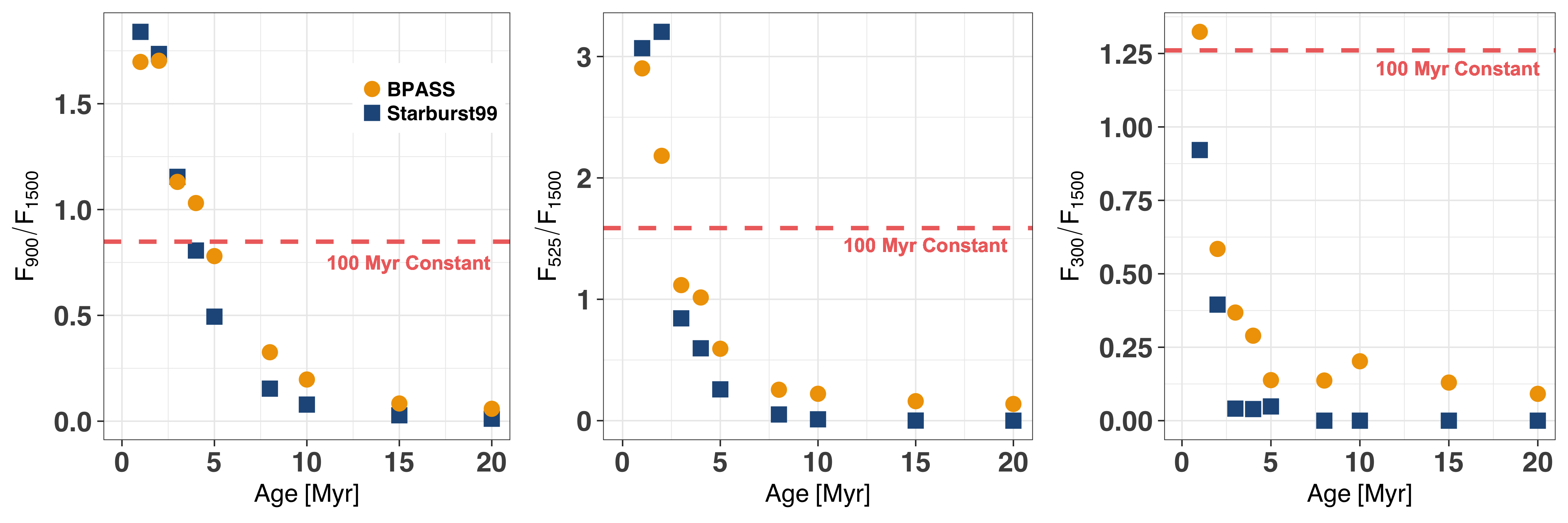
We use three different ionizing to non-ionizing flux density ratios to quantify the shape of the ionizing continuum (F900/F1500, F525/F1500, F300/F1500). As hinted in Figure 12, the left panel of Figure 13 shows a smooth temporal trend of F900/F1500 with age at a fixed metallicity. Higher energy photons (probed by the flux density ratio of F525/F1500) have a similarly strong temporal evolution (middle panel of Figure 13), but shifted to earlier ages, such that only stars younger than 5 Myr are sufficiently hot to emit appreciably at 525Å. The ionizing continua of the youngest stars peak near 525Å where F525 is three times more luminous than F1500. Finally, the highest energy photons (probed by the flux density ratio of F300/F1500) are exclusively produced by stellar populations with ages less than 2 Myr (right panel of Figure 4). The flux density ratios of theoretical starburst99 models show that the stellar age correlates with the shape and strength of the ionizing continua.
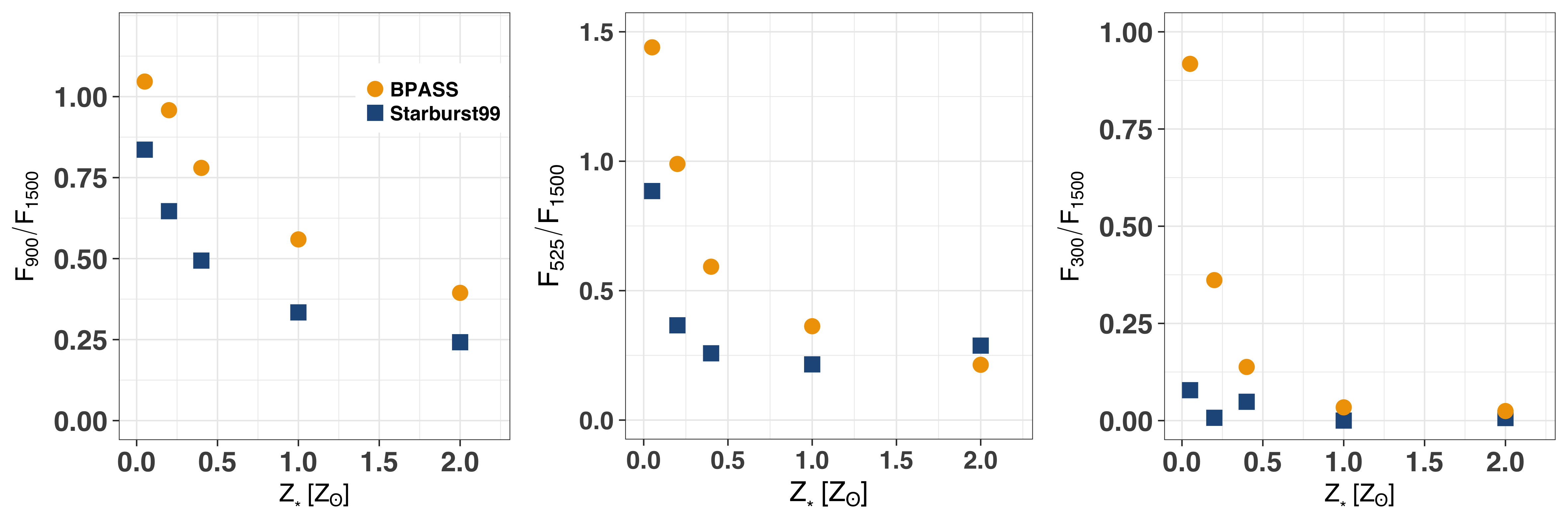
The stellar metallicity (Z∗) also impacts the shape of the ionizing continuum as measured by the flux density ratios (Figure 14; Smith et al., 2002). At a constant stellar age of 5 Myr, the F900/F1500 increases by a factor of 3 as Z∗ decreases by a factor of 40 (left panel of Figure 14). Similarly, F525/F1500 and F300/F1500 decrease by a factor of three and twelve from Z∗ = 0.05 to 2 Z⊙, respectively. The ionizing to non-ionizing flux density ratios also quantify the impact of Z∗ on the shape and strength of the stellar ionizing continua.
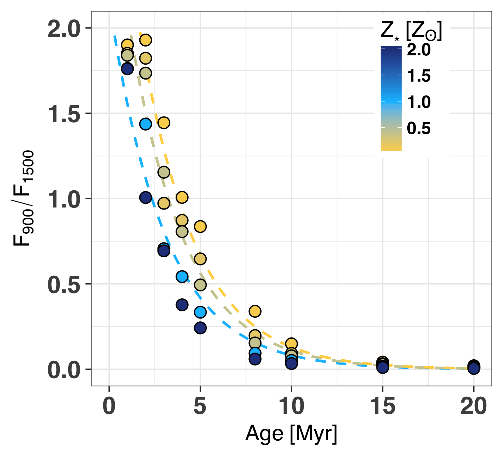
Figure 15 illustrates that both the stellar population age and metallicity impact the ionizing continuum. A multivariate, robust M-estimator linear regression (Huber, 1981) finds a relationship between these three variables for the single burst starburst99 models (only including ages Myr) as
| (5) |
This relation determines the ratio of the intrinsic ionizing flux density at 900Å to the non-ionizing flux density at 1500Å for a single age burst of star formation given the stellar population age and metallicity.
In Figure 15, we use Equation 5 to overplot three curves of constant Z∗ onto the full starburst99 grid. The curves generally approximate the variations in the models, but there still exists real variations at a given age. F900/F1500 evolves significantly at the youngest ages and small measurement errors lead to large F900/F1500 errors. The median error of the estimated age and Z∗ is 13% and 11% of the estimated values, respectively. For an estimated age of 3 Myr and metallicity of 0.4 Z⊙, with these median uncertainties, there is a 15% uncertainty on F900/F1500, including calibration errors. The median MegaSaura SNR, 21, is high for restframe FUV observations, but extremely high-quality observations are required to determine F900/F1500, even with a 15% error.
The F900/F1500 scales strongly with both stellar age and metallicity because both impact the stellar temperature. As stellar populations age, their stellar temperatures decrease which increases the fraction of neutral hydrogen within the stellar atmospheres. This is observed in the optical where Balmer absorption lines increase in older B and A-stars. Thus, the rapidly evolving F900/F1500 ratio with stellar age and Z∗ in Figure 15 probes the increasing X(H0)/X(H+) ionization fraction within the stellar atmospheres with decreasing stellar temperature. By the time the stellar population ages to 15 Myr, the temperature has dropped below 20,000 K and there is sufficient neutral hydrogen within the stellar atmospheres to absorb all of the ionizing photons. Thus, F900/F1500 traces the hydrogen ionization fraction within the stellar atmospheres.
5.2.2 Inferred ionizing continua from observed galaxies
We inferred the ionizing continua of the observed massive star populations by extending the stellar fits blueward beyond the observations. The fits are linear combinations of multiple single age models, and therefore the inferred ionizing continua may be more complicated than the single burst relations presented in Section 5.2.1. How much do the inferred continua depart from a single burst model?
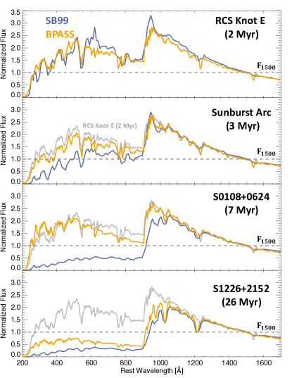
In Figure 16, we show the inferred ionizing continua of four galaxies that span the full age range of the sample. Focusing on only the starburst99 fits (blue lines), the general trend found in Figure 12 is reproduced: the inferred ionizing continua at 900Å decreases with fitted stellar age from RCS Knot E (top panel; 2 Myr), to the Sunburst Arc (top-middle panel; 3 Myr), to S0108+0624 (bottom-middle panel; 7 Myr), and finally S1226+2152 (bottom panel; 26 Myr). The galaxies with the strongest inferred ionizing continua are the youngest galaxies with the strongest stellar wind profiles (Section 4).
At wavelengths blueward of 900Å, the starburst99 inferred ionizing continua have substantially different morphologies. The ionizing continuum of RCS Knot E increases from 900 to 525Å, the Sunburst Arc stays relatively flat from 900 to 525Å, while the ionizing continua of S0108+0624 and S1226+2152 both decline with decreasing wavelength. The inferred shapes of the ionizing continua constrain the total number of ionizing photons produced by the stellar population and the hardness of the nebular emission spectra (see Section 5.7). In this parlance, RCS Knot E has a particularly hard ionizing spectrum, while S1226+2152 has a relatively soft spectrum.
The inferred F900/F1500 qualitatively follows the general trends outlined in Section 5.2.1. RCS Knot E is the youngest population and has a F900/F1500 that is 5 times larger than the oldest galaxy, S1226+2152. However, there are large departures in the inferred F900/F1500 values from the single burst models: S1226+2152 has a light-weighted age of 26 Myr, yet it still has a F900/F1500 . S1226+2152 has an old stellar population, the C IV profile is nearly flat (Figure 4), yet the inferred ionizing continuum is 500 times stronger than a single burst model with the same age and metallicity (F900/F1500 = 0.0006). Similarly, S15270652 and the Cosmic Eye have light-weighted ages of 21 and 29 Myr but inferred F900/F1500 of 0.2 and 0.1, respectively. These values are 50 and 400 times larger than predicted by the single burst models. This over-production of ionizing photons extends to all populations older than 9 Myr.
Whether the inferred ionizing continua agree with the single burst models splits the observed stellar populations into two star formation histories: a single burst and a mixed age population (Figure 17). Bursts have stellar ages less than 8.6 Myr, while mixed age populations have ages greater than 8.6 Myr. This divides the full sample into 31 burst-dominated stellar populations and 30 mixed age populations. There is not a statistical redshift dependence as both the low-redshift sample and the MegaSaura sample are nearly split evenly.
We overlay the single population model tracks of Figure 15 onto the inferred F900/F1500 in Figure 17 to show that young populations have single burst-dominated ionizing spectra. All of the burst-dominated non-ionizing spectra have the spectral properties outlined in Section 4.3 for young stellar populations: strong N V and C IV P-Cygni features, broad He II emission (when the transition is within the wavelength coverage), and non-detected Si III photospheric features.
The spectra of the second population are a mixture of old and young stellar populations. The stellar continua of these stellar populations are complex, with contributions from young stars shaping the stellar winds and B-stars contributing photospheric absorption features.This creates an averaged ionizing continuum that is non-zero due to contributions from massive O-stars, but diluted by contributions from older populations.
The spectral differences between the two populations are seen by comparing the C IV features of the burst-dominated RCS Knot E and the mixed age S12262152 in Figure 4. RCS Knot E has very strong and pronounced C IV absorption and emission profiles, similar to the single age starburst99 model. Meanwhile, single burst models do not fit S12262152: the 20 Myr single age C IV profile under-estimates the C IV absorption and emission, indicating a weak O-star population. Besides this weak O-star contribution, the pronounced photospheric absorption clearly indicates an older B-star population (Figure 9). The observed spectral features demonstrate that as the inferred light-weighted age increases, a single stellar population ceases to dominate the stellar continuum, rather the stellar light becomes a mix of young and old spectral features.
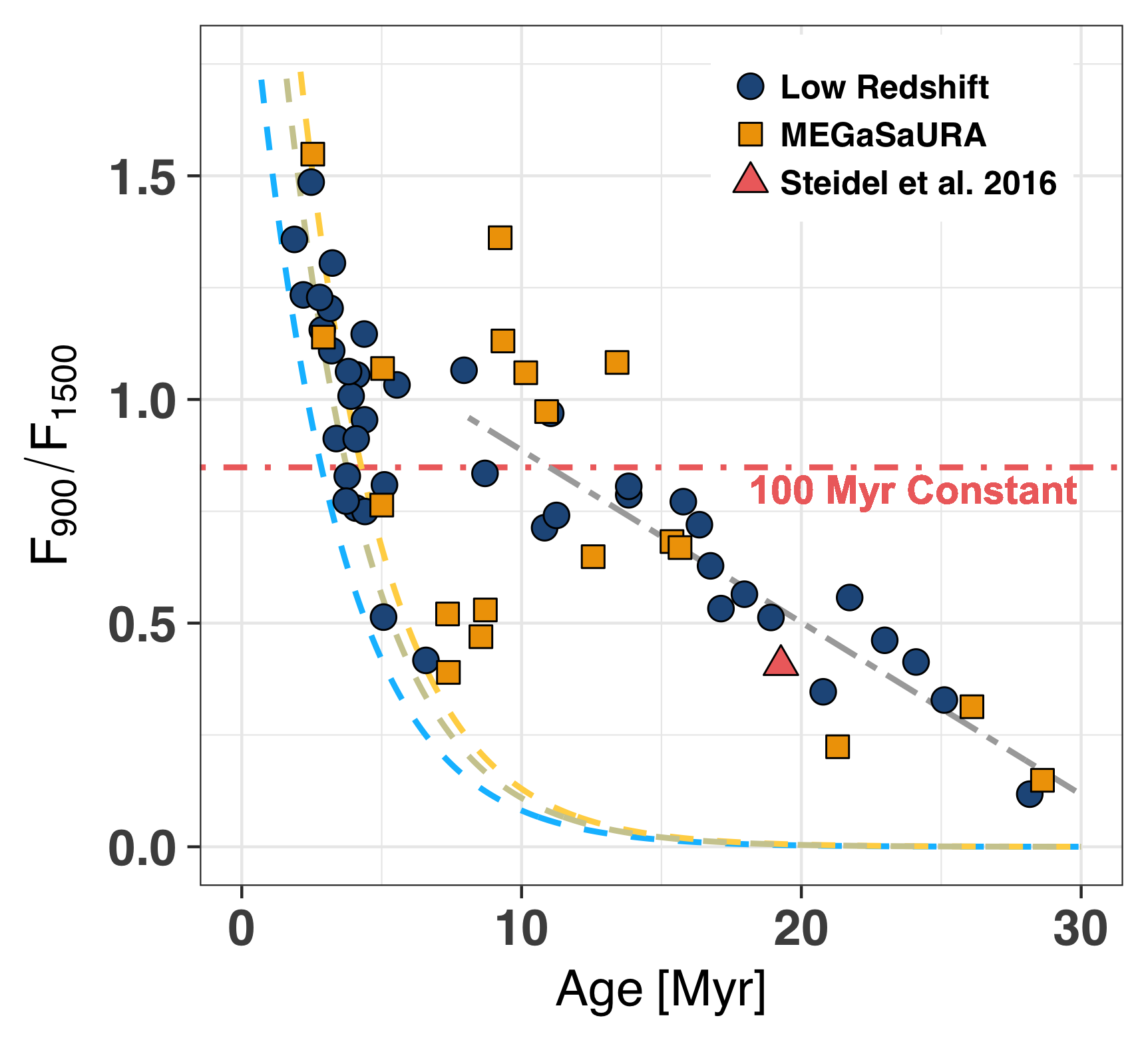
In Figure 17, the F900/F1500 of the mixed age population strongly (5.5, Pearson’s correlation coefficient of ) and linearly decreases with light-weighted age between 8-30 Myr as
| (6) |
This relationship is overplotted on the observations in Figure 17 as a gray dot-dashed line. There is not a statistically significant trend between F900/F1500 and Z∗, such that the statistical significance of the trend decreases if we introduce a multivariate fit. Equation 6 analytically quantifies the evolution of the strength of the ionizing continua of older mixed aged stellar populations.
We investigated the origin of mixed age populations by envisioning that the observations of individual star-forming regions sample a random mixture of stellar populations at various ages. This can be analytically tested using a random assortment of the theoretical stellar models. The model grid contains more young stars because their spectral features vary on shorter timescales, consequently, for modeling purposes, we only included starburst99 models with ages less than 4 Myr or greater than 10 Myr. We then simulated whether a burst occurred using a binomial distribution with a uniform probability of success for each model. We chose the probability for success to be 15% such that the expected value of the number of bursts matched the number of models typically included in the fits (). The success probability was tested for a range between 1-50%, but the results were not sensitive to the chosen probability. If the random binomial for a given model returned a success (P() = 1), we assigned a random light-fraction drawn from a Gaussian distribution. This process was repeated for all possible stellar models and the sum of all light-fractions was normalized to total one. We multiplied the stellar models by the randomized light-fractions and summed the synthetic stellar populations according to Equation 1. We inferred the light-weighted age and F900/F1500 using the same method as for the observations. We then repeated this process one million times to create a statistical sample of random mixtures of stellar populations. This sample of synthetic observations is hereafter referred to as the MCMC sample. We found a strong correlation (Pearson’s correlation coefficient of ) between the age and the F900/F1500 of this random mixed age population to be
| (7) |
This relationship is statistically similar to the relationship inferred from the mixed age population in Equation 6. This suggests that older inferred light-weighted ages are composites of multiple epochs of stellar populations within a single aperture. A single stellar population does not dominant the FUV light of mixed age populations, rather the FUV light is broadly distributed distributed over many ages. The resultant composite is a detailed, light-weighted mixture of the different epochs of star formation.
The relative proportions of this age mixture are determined by the light-fraction of each model at a given age, or (where is the light-fraction of each model age; see Equation 1). As a simplified example, assume that the light at 1270Å of a 0.4 Z⊙ stellar population comes 70% from a 2 Myr population () and 30% from a 25 Myr population (). The light-weighted age from Equation 3 is 8.9 Myr and the light-weighted F900/F1500 from Equation 5 is 1.05. These inferred values are on the age-F900/F1500 mixed age relationship of Equation 6. The 8.9 Myr stellar continuum has a deep N V profile from the 2 Myr population, but weak photospheric lines from the 25 Myr population. This hypothetical stellar population resembles RCS Knot G in Figure 4 which is dominated by light-fractions of , , and of 0.30, 0.43, and 0.20, respectively. If the assumed light-fractions of the toy model are reversed, the light-weighted age increases to 18 Myr and F900/F1500 decreases to 0.45. The younger population contributes less to the integrated stellar light and the stellar wind lines of this older hypothetical population are now flatter, resembling S1429-1202 in Figure 6. The observed stellar populations are more complicated than these toy examples, but they illustrate the evolution of the ionizing continua of mixed age populations.
The ionizing continuum of a mixed age population looks very different than that of a single burst. A single burst 8 Myr, 0.4 Z⊙, starburst99 population has F900/F1500 and F300/F1500 , but the mixed age population envisioned above has F900/F1500 and F300/F1500 . This “old” mixed age stellar population produces six times more photons per F1500 than a single burst of the same age. Moreover, mixed age populations produce a large number of extremely hard ionizing photons due to their out-sized presence of very young stellar populations (in this example ). Similarly, the 18 Myr population theorized above has an F300/F1500 that is still three times larger than a single burst 3 Myr stellar population, among the youngest in our sample, even though the stellar age inferred from the non-ionizing continuum is five times older. Mixed age stellar populations produce dramatically more ionizing photons than suggested by their light-weighted ages.
The fitted light fractions illustrate the difference between a population dominated by a single burst and a mixture of bursts (see Figure 2). RCS Knot E has a burst-dominated stellar spectra with a light-weighted age of Myr. 100% of the FUV light comes from populations with ages less than 4 Myr (and %; left panel of Figure 2). Alternatively, S1527+0652 has a mixed age stellar spectra with a light-weighted age of Myr. Young stellar populations (¡5 Myr) within S1225+2152 contribute 19% of the FUV light, while older stellar populations supply 81% of the FUV light (where the dominate ones are and with 31 and 44%, respectively). The age distribution of burst populations is relatively simple and clustered, but the light from mixed age populations is broadly distributed over many stellar ages.
A principle worry is whether the derived continuum fits, and the associated mixed age populations, are robust. The errors on the stellar properties were derived by varying the observed flux of the stellar continuum by a random Gaussian with a width equal to the observed flux uncertainty and then refitting the stellar continuum. This process was repeated 100 times and the standard deviation of the ensemble was taken as the stellar property uncertainty. We find that the SNR of the parameter scales with the spectral SNR at the 3 significance (p-value of 0.0006, Kendall’s value of 0.65). As a general guide, we find that the median SNR of the inferred stellar population age is 0.44 times the observed spectral SNR per resolution element. Thus, a spectral SNR per resolution element of 22 (7) is required to determine the stellar age at the 10 (3) significance level. In Section 5.2 we also noted that a spectral SNR of 21 estimates the F900/F1500 with a 15% uncertainty. Thus, a SNR is a general guideline to robustly determine the stellar population properties and to infer the ionizing continua.
If the age mixtures were arbitrary mixtures that were not constrained by spectral properties, then we would measure a different fitted age for each iteration and the inferred age and metallicity uncertainty would be largely unconstrained and uncorrelated with the spectral SNR. We conclude that the properties of both single bursts and mixed age populations are relatively robust and constrained by spectral signatures.
5.3 Mixed age versus continuous star formation histories
In Section 4 we emphasized that the O and B-star spectral features reflect changes in the inferred stellar population age and metallicity. In Figure 3, we showed that the stellar wind lines are sensitive to the age of the stellar population. Young populations show strong C IV P-Cygni emission, while older stellar populations have more moderate C IV features. The N V wind feature only depends on age (Figure 3) and we see strong galaxy-to-galaxy N V variations (Figure 6). Short-lived Wolf-Rayet stars create a broad He II feature that is only seen in the youngest (¡5 Myr) spectra (Figure 8). Similarly, older stellar populations have weak, but distinct, photospheric absorption features that are absent in the youngest stellar populations (Figure 9). We concluded that there is real and quantifiable age variation within the observed stellar continua.
The stellar continua vary from galaxy-to-galaxy, but not always as predicted from a single stellar population. The stellar wind profiles from populations with older light-weighted ages require a mixture of ages (see S1226+2152 in Figure 4). This mixture extends to the ionizing continua, where Figure 17 demonstrated that the inferred ionizing spectra are divided into two star formation histories: single bursts and mixed age populations. A mixed age stellar population contains some assortment of young (¡5 Myr) and old (¿8 Myr) stellar populations that varies from galaxy-to-galaxy.
Constant star formation is the canonical alternative to a single burst star formation history. A constant star formation history assumes that every year a fixed number of stars are formed by consistently populating the IMF. When averaged over a sufficiently long temporal baseline (100 Myr, similar to the ages of older B-stars), continuous star formation is a good physical description of the star formation history of evolved star-forming galaxies, such as normal spirals. However, it is unlikely that stars with lifetimes 1-10% of the dynamical time of galaxies will form at a constant rate. However, in principle, a constant star formation is a singular, simplified mixed age solution that can be recovered with the proper light-fractions.
A constant star formation history has a fixed number of O-stars which produce a fixed number of ionizing photons. The red lines in Figure 13 show the ionizing flux density ratios of a 0.05 Z⊙ bpass constant star formation model. This constant star formation law is similar to a mixed age population with an age of 12 Myr (Figure 17), but a continuous star formation history under-predicts the ionizing continuum of a 8 Myr mixed age population by a factor of 2, and over-predicts the ionizing continuum of a 25 Myr mixed age population by a factor of 3 (Figure 17). The number of ionizing photons produced by a constant star formation history only matches the inferred ionizing continua of the mixed age fits near 12 Myr, and a constant star formation history does not match the ionizing continua at other stellar ages.
Only Z∗ can change the stellar continuum of a constant star formation history. Predominately age sensitive tracers, such as N V and the ionizing continuum, have fixed strengths in a constantly star-forming model. A constant star formation model may fit part of the C IV absorption profile well, but over (or under) estimate the N V profile because the age has been fixed (see Figure 3). The constant star formation model fails to simultaneously fit the different stellar wind profiles of very young populations (e.g. the Sunburst Arc in Figure 6) or older populations that lack stellar wind signatures (e.g. S1527+0652 in Figure 6).
Unlike continuous star formation histories, FUV spectral features determine the mixed age star formation histories and observationally constrain the relative contributions of young and old stars. By accounting for the dominance of young stellar populations to certain ionizing continua, mixed age star formation histories generate significantly more ionizing photons, at higher energies, than continuous star formation histories. The different star formation histories alter the ionizing continua by factors of 2–3 and must be determined to accurately infer the number of ionizing photons produced by stellar populations.
5.4 Impact of binary evolution on the stellar continua
Most massive stars form in binaries (Sana et al., 2012), and mass can be transferred between the two stars if they are sufficiently close. The star that receives the mass is rejuvenated and its main-sequence lifetime is extended (Eldridge & Stanway, 2009; Götberg et al., 2017). Mass transfer typically occurs when one star is in an evolved stage and expands to fill the Roche lobe. Consequently, binary star evolution extends the duration that stars spend in late evolutionary phases such as the Wolf-Rayet phase (Vanbeveren et al., 2007; Georgy et al., 2012). By increasing the pathways to form evolved stars, populations with binary evolution emit more ionizing photons and have harder ionizing spectra than populations with only single star evolution (Stanway et al., 2016; Götberg et al., 2017, 2018). Binary evolution establishes a significant evolved population at lower metallicities because lower metallicity stars are hotter and must expand more in their later evolutionary phases. On the other side of mass transfer, the star that donates its hydrogen envelope is hypothesized to remain as an extremely hot helium core with a black body that peaks blueward of 912Å, possibly as an X-ray binary (Van Bever & Vanbeveren, 2000; Mirabel et al., 2011; Fragos et al., 2013; Götberg et al., 2017). These processes add an additional source of extreme ionizing radiation.
Binary star evolution drastically increases the number of ionizing photons produced by a stellar population. Can the rest-frame FUV observationally constrain the importance of binary evolution? Here we discuss the observational differences between bpass and starburst99 models in their non-ionizing spectra (Section 5.4.1), the differences between the derived stellar population properties (Section 5.4.2), and then compare the ionizing continua of the two evolution models (Section 5.4.3). We conclude that the non-ionizing continua alone cannot discern the impact of binary evolution, and explore alternative observational methods to distinguish between binary and single star models (Section 5.4.4).
5.4.1 Does binary evolution change the observed non-ionizing stellar continuum?
starburst99 and bpass predict comparable non-ionizing continua (see Figure 1). The two use similar O-star libraries and produce largely identical non-ionizing spectral features. The stellar wind shapes (e.g. N V and C IV) slightly differ, but this reflects the subtle differences in the O-star models rather than the impact of binary evolution (Leitherer et al., 2010; Conroy et al., 2014; Eldridge et al., 2017). The SNRs of individual galaxies are typically too low to distinguish between the two stellar models (compare the blue and gold lines in Figure 4–6). However, the starburst99 models fit the N V and C IV wind features of the high SNR (SNR = 103 per resolution element) MegaSaura stack marginally better than the bpass models (Rigby et al., 2018b).
bpass and starburst99 have significant differences in their older populations. The C III and Si III 1299Å photospheric features, which we identified in Section 4.2 as strong B-star diagnostics (de Mello et al., 2000), are very weak in the bpass models (Figure 1). This is likely due to the fact that bpass models below 20,000 K have lower spectral resolution at wavelengths less than 1500Å and the weak absorption lines are nonphyiscally blended into the continuum (see the red 15 Myr model in Figure 1). The absence of C III and Si III absorption features is likely due to the inadequate spectral resolution, not binary star evolution.
The broad stellar He II emission is more prominent in 5-8 Myr bpass models than starburst99 models (Figure 1; Steidel et al., 2016). The bpass models do fit the He II region substantially better than the starburst99 models, but the overall fit is still occasionally poor at young ages (Figure 8). This is likely because binary evolution provides an additional pathway to create and rejuvenate WR-stars such that the bpass models contain more evolved stars, but either the WR evolution or atmosphere models still need refinement. The improved fit of the He II region may indicate that binary stars contribute to the FUV light, but even the bpass fits do not completely describe the He II region.
Similarly, the increased population of evolved massive stars produces Si IV P-Cygni that are stronger than the C IV features at ages of 5–10 Myr (Figure 1). Differences between Si IV stellar wind profiles are a key prediction of models that do and do not include binary evolution. Si IV is not prominently observed as a stellar P-Cygni profile at low Z∗, but Figure 7 shows that the fitted Si IV profiles are statistically similar whether bpass or starburst99 models are used. Even though the single age bpass models show broad Si IV P-Cygni profiles, the multiple age fits do not indicate Si IV P-Cygni features. This is because the population is a mixed age population with young (¡5 Myr) and old (¿10 Myr) populations rather than a single age 8 Myr population. Thus, the non-ionizing stellar continua do not disentangle the impact of binary star evolution on the ionizing continua.
5.4.2 Does binary evolution impact the inferred light-weighted stellar ages and metallicities?
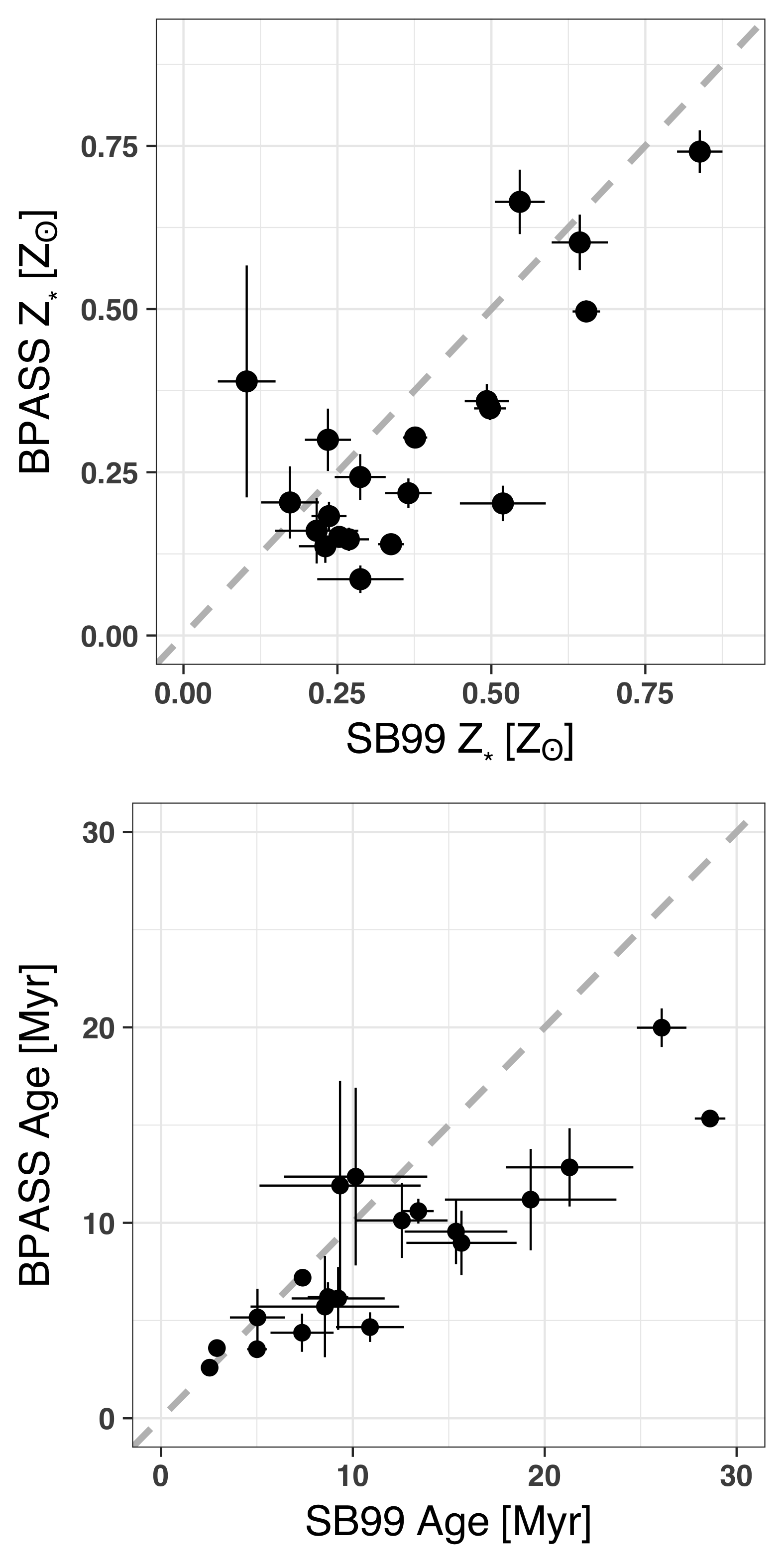
The light-weighted metallicities and ages derived with bpass and starburst99 in Figure 18 are similar. However, bpass models have a lower spectral resolution at wavelengths Å for stellar temperatures ,000 K. This means that the bpass models do not have a single spectral resolution over the bandpass. This biases the COS fits either toward younger stellar populations where the spectral resolution matches the data or towards older populations where multiple individual features are combined into single unresolved features. These resultant bpass fits to the COS data often times do not match the N V stellar wind profiles. We tested that the reduced wavelength coverage causes the poor fitting of the COS data by fitting the MegaSaura data with only rest-frame wavelengths Å. We found that the bpass fits to the MegaSaura data with only wavelengths ¡1500Å were similarly poorly fit by the bpass models, but the starburst99 fits were not impacted by using the restricted wavelength regime. Consequently, we only compare the bpass fits for the MegaSaura data, which have a complete wavelength coverage.
The inferred light-weighted stellar metallicities (at the significance) and ages ( significance) scale along the one-to-one relationship in Figure 18. The ages are similar for young populations (¡15 Myr), while bpass models systematically estimate younger ages when starburst99 ages are ¿15 Myr. This split happens at the same age as the degradation of the bpass spectral resolution discussed above. Thus, we conclude that, while the poor bpass spectral resolution inhibits a firm conclusion, the ages and Z∗ derived using the different stellar models are similar. In the next section, we compare the bpass ionizing continua, but we note that the inferred bpass ages are up to 30% younger for the oldest populations.
5.4.3 Binary evolution strongly impacts the ionizing continua
The C IV (Figure 4 & 5) and N V (Figure 6) regions cannot discriminate between binary and single star populations. While bpass models fit the He II region better than starburst99 models (Figure 8), neither successfully reproduces the full He II spectral shape. We concluded that the fitted non-ionizing continua cannot determine the contribution of binary star evolution to the stellar continuum.
Conversely, the bpass modeled ionizing continua drastically differ from the starburst99 continua. This is most extreme for older and lower metallicity stellar populations (Figure 13 14). At young ages (¡3 Myr), the production of ionizing photons is similar regardless of the binary evolution model because young stars have not yet evolved off the main-sequence. Meanwhile at older ages, such as 8 Myr, there is a factor of two difference in F900/F1500 between bpass and starburst99 models. This difference is similar to the difference between a burst and a 8 Myr mixed age population (Section 5.2.2).
The modeled ionizing continua differ most drastically at higher energies (right two panels of Figure 13). A single 10 Myr starburst99 burst has negligible F300/F1500 , but a population that includes binary evolution produces a staggering F300/F1500 (the furthest right circle in the right panel of Figure 12). Populations with binary evolution have substantially harder ionizing spectra due to the enhanced contribution of evolved stars.
Thus, the inferred bpass ionizing continua are typically stronger and harder than those inferred from starburst99 (blue versus gold curves in Figure 16). While the bpass models exhibit the same qualitative trend of decreasing F900/F1500 with inferred stellar age, there are important differences between the ionizing continua inferred with bpass and starburst99. RCS Knot E (top panel) has the youngest MegaSaura population (2.5 Myr) and the inferred ionizing continuum is similar for both starburst99 and bpass models. Conversely, the Sunburst Arc, which is only 0.5 Myr older, has similar F900/F1500 values, but the F525/F1500 and F300/F1500 are 1.4 and 4.9 times larger for the bpass models than the starburst99 models, respectively. The oldest galaxy, S12262152, again has the lowest F900/F1500, but F900/F1500, F525/F1500, and F300/F1500 are 1.4, 2.0, and 7.2 times larger for the bpass models than the starburst99 models.
S01080624 has the most pronounced difference in the bpass and starburst99 ionizing continua. The inferred F900/F1500, F525/F1500, and F300/F1500 are 2, 4, and 12 times larger for the bpass fits than starburst99. Surprisingly, the bpass models in Figure 16 predict larger F300/F1500 for the older population of S01080624 than the youngest stellar populations in the sample, such as RCS Knot E (1.4 times larger) and the Sunburst Arc (1.7 times larger).
The inferred ionizing continua of stellar populations that include binary evolution can produce up to 12 times more hard ionizing photons per FUV luminosity than single star populations with the same FUV spectral features. This presents an uncomfortable conclusion: there is up to an order of magnitude difference in the number of ionizing photons predicted from populations with binary evolution that cannot be observationally constrained by the non-ionizing stellar continuum. Additional observations must constrain the impact of binary star evolution.
5.4.4 How to observationally distinguish binary and single star populations
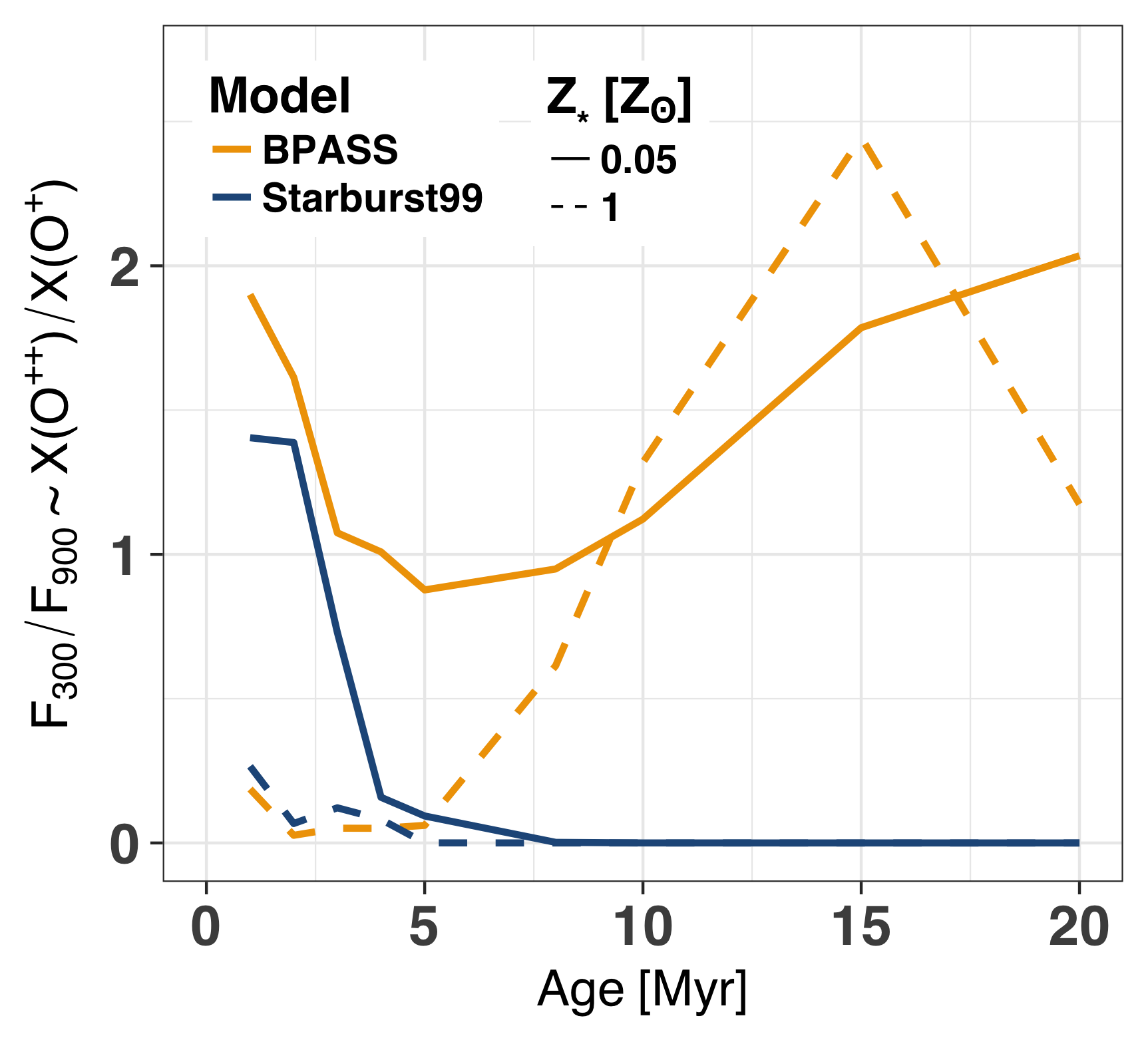
The previous sub-sections demonstrated that the non-ionizing stellar continua cannot quantify the impact of binary star evolution on the integrated stellar spectra, but there are extreme differences in their respective ionizing continua. While observations suggest that massive stars typically form in binaries, the exact binary parameters–mass ratios, period distributions, and remnant masses–are largely unknown and must be assumed to create the bpass models (Eldridge et al., 2017). Therefore, the impact of binary evolution on the stellar continuum is observationally unconstrained. Observational tests must break this degeneracy.
Direct observations of the extreme-UV continuum (EUV; wavelengths ¡912Å) are a definitive method to break this degeneracy. With up to a factor of 12 flux density difference between the bpass and starburst99 modeled ionizing continua, direct observations would indisputably determine the impact of binary star evolution on the ionizing continuum. Further, there are strong stellar wind lines in the EUV (e.g. N III 763Å) which are more prevalent in binary populations than single star populations (Figure 16). The intrinsic LyC break (near 912Å) is also different for 5–10 Myr populations due to the higher stellar temperatures of binary populations (Figure 12). However, the EUV of an O-star dominated stellar population has never been observed.
Steidel et al. (2016) broke this degeneracy using nebular emission lines. For an ionization bounded nebula (or where the gas absorbs all of the ionizing photons), the relative strength of nebular emission lines at different ionization states (e.g., [O III] 5007Å versus [O II] 3727Å) traces the intrinsic hardness of the stellar spectrum, and H and He recombination lines trace the intensity (normalization) of the ionizing continuum (modulo the escape of ionizing photons and the effects of dust). Constraining whether the inferred bpass or starburst99 ionizing continua better reproduce the observed nebular emission line structure will illuminate the importance of binary evolution.
Comparing [O III] and [O II] emission lines may resolve the different ionizing continua of the two evolutionary models. bpass models create more more O++ gas relative to low ionization, O+, gas than single star models (Stanway et al., 2014). We illustrate this by comparing the F300/F900 ratio of the starburst99 (blue lines in Figure 19) and bpass models (gold lines in Figure 19). Photons at 300Å produce O++ gas, while photons at 900Å only generate O+; F300/F900 probes the formation of O++ and O+ gas which emit [O III] and [O II], respectively. This is meant to illustrate the possibility of observing differences in the [O III]/[O II] ratio with stellar age, but full photoionization modeling is required to compare to the observed emission lines. Models without binary evolution produce O++ at low metallicities and young ages, while bpass models produce large X(O++)/X(O+) ratios at all metallicities and ages. In fact, high Z∗ bpass models produce larger X(O++)/X(O+) ratios than the youngest low-metallicity single star models. Correlations between X(O++)/X(O+) and stellar population properties may constrain the importance of binary evolution.
Individual emission lines may also break the degeneracy between binary and single-star models. Nebular He II emission requires extremely high-energy photons (Å). Stellar continua are typically considered too weak and too soft to reproduce the observed He II 1640Å and He II 4686Å nebular emission (Kehrig et al., 2015; Berg et al., 2018; Nanayakkara et al., 2018; Stanway & Eldridge, 2018a; Schaerer et al., 2019). S01080624 is the only spectrum in the MegaSaura sample with a weak and narrow He II emission line (Figure 8; equivalent width of Å). Figure 16 shows that the bpass fit to S01080624 has a harder spectrum than the youngest stellar populations (compare the gold and gray lines in the third panel), possibly suggesting that evolved, mixed age binary star populations are required to produce the observed nebular He II.
5.5 Fits to stacked MegaSaura spectra
Stacking, or averaging many spectra together, increases the SNR of the composite spectrum. Often it is assumed that a stacked spectrum probes the average properties of the underlying population. The combination of the high-quality individual MegaSaura spectra and the stacked MegaSaura spectrum allows us to test this hypothesis.
By weighting the individually measured stellar ages and metallicities by the SNR of their respective MegaSaura spectrum at 1500Å, we estimated the stellar age and metallicity of the MegaSaura ensemble to be Myr and Z⊙ ( Myr and Z⊙ for bpass). We then fit the stacked MegaSaura spectrum and estimated a light-weighted age and metallicity of Myr and Z⊙ ( Myr and Z⊙ for bpass). Thus the inferred stellar properties of the stack are statistically similar to the ensemble averages.
The SNR weighted average F900/F1500 of the individual fits is and the inferred F900/F1500 from the stack is 0.47. Meanwhile, if we input the fitted light-weighted age of the stellar population into the F900/F1500 relationship (Equation 6), we expect F900/F1500 . We find that the fitted stellar properties of the MegaSaura stacked spectra reasonably match the underlying population averages.
5.6 Comparison to previous work
The most directly comparable work to our stellar population synthesis fitting is Steidel et al. (2016). Those authors used a stack of 30 galaxies at with rest-frame FUV and optical observations (for the optical emission lines) to determine the stellar population and nebular emission properties. They fit a variety of Z∗, IMFs, and stellar models (bpass versus starburst99) to the observed stellar continuum, but always used a continuous star formation history. Low metallicity ( Z⊙) continuous star formation models fit the stellar continuum best, even though the measured nebular metallicities were Zneb = 0.29–0.49 Z⊙.
The various continuous star formation stellar continuum models were then used as the ionizing source within cloudy photoionization models to predict the nebular emission lines and compare these predictions to the observed values. Continuous star formation starburst99 models produced an insufficient number of ionizing photons to match the observed classical Baldwin et al. (1981) diagnostics such as [O III] 5007Å/H and [N II] 6585Å/H. Similarly, bpass models with Z∗ = Zneb failed to reproduce these nebular emission-line ratios.
However, Steidel et al. (2016) could reproduce the emission lines if Z∗ was five times smaller than Zneb. Steidel et al. (2016) argued that rather than a lower Z∗, the /Fe relative abundance ratio of galaxies must be super-solar. This would lead to a measured Z∗ that is smaller than the actual metallicity, and the stars would produce more ionizing photons because Fe is the chief opacity source in the atmospheres of massive stars. Thus, they concluded that the non-solar /Fe relative abundances produced an illusion that the stars had five times fewer metals than the gas.
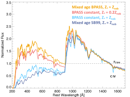
We fit the Steidel et al. (2016) stack with the methods outlined above, and derived a light-weighted Z∗ = 0.37 Z⊙ using starburst99 models ( Z⊙ using bpass). The inferred starburst99 stellar population age of the Steidel et al. (2016) stack is 12.6 Myr, implying that it is a mixed age population. These metallicities are similar to the nebular metallicities of Zneb = 0.29–0.49 calculated using the direct and strong-line methods, implying that the stars and gas have similar metallicities (we plot both the direct and strong-line Zneb calculations in Figure 11).
While the inferred light-weighted Z∗ is meant to convey a total metal content, the strong stellar wind lines, which are only observed through -element transitions in the FUV, could hide discrepant /Fe abundance ratios (Steidel et al., 2016). Therefore, Steidel et al. (2016) suggested using regions devoid of strong wind features, but containing many weak photospheric lines (the so-called “featureless” regions in Table 2) to test the stellar Fe abundance. Using “Mask 2” from Steidel et al. (2016), we refit their composite spectra using only wavelengths without strong stellar wind lines and find a very similar light-weighted Z∗ as when we fit the entire spectrum (0.43 and 0.37 Z⊙ for starburst99 and bpass, respectively). Thus, even in stellar spectral regions dominated by Fe absorption features, we still infer that Z∗ and Zneb are similar.
The only difference between the inferred Z∗ from this work and Steidel et al. (2016) is the assumed star formation history. As emphasized in Section 5.3, a constant star formation history predetermines a fixed number of young and older stars, each with their own distinct spectral signatures. Since young populations have Fe IV and Fe V photospheric lines (Figure 1) and slightly older populations generally have Fe III lines (fig. 5 in de Mello et al., 2000), a continuously star-forming population is always expected to have Fe III, Fe IV, and Fe V absorption. The assumption of constant star formation may force the Steidel et al. (2016) fits toward lower metallicities in order to balance the strength of the Fe absorption across different ionization states. By contrast, a mixed age stellar population can reduce the Fe absorption lines by either reducing the metallicity or by selecting the proper combination of stellar population ages to match the observed Fe lines (i.e. an older population without Fe IV and Fe V or a younger population without Fe III). Thus, we emphasize that the a priori assumed star formation history (constant versus mixed age) has a profound impact on the inferred stellar metallicity.
Even though the light-weighted Z∗ derived from our mixed age fits to the stellar continuum are four times larger, the C IV 1550Å stellar wind P-Cygni profile appears similar to the lower metallicity, 0.05 Z⊙ continuous star formation model (orange and red lines Figure 20) and weaker than the 0.3 Z⊙ constant star formation model (light blue line). As discussed in Section 5.3, continuous star formation models remove possible age variations, leaving Z∗ as the only lever to influence the C IV P-Cygni shape. The mixed age fits to the stacked data have light-weighted ages of Myr using starburst99 ( Myr using bpass) such that a moderate metallicity, moderate age population has relatively weak C IV absorption.
Figure 20 shows the inferred ionizing continuum from the fit to the Steidel et al. (2016) stack. This figure strongly emphasizes that mixed age populations produce substantially more ionizing photons, even at higher metallicities, than continuous star formation models. The starburst99 fit (dark blue line) has a weaker ionizing continuum than the bpass fit (orange line), and the starburst99 fit is more similar to the bpass Z∗ = Zneb continuous star formation model (light-blue), which failed to reproduce the nebular emission. As suggested by Steidel et al. (2016), the starburst99 fits are unlikely to generate sufficient ionizing photons to match the nebular emission.
The bpass mixed age fit to the stack (orange curve in Figure 20) produces more ionizing photons, with a similar spectral shape, as the low metallicity continuous star formation model which reproduced the nebular emission structure (red curve). The youngest stellar populations produce the most ionizing photons (Figure 15), thus, allowing younger populations to have larger light-fractions increases the total number of ionizing photons produced by a stellar population (see Section 5.7). Consequently, a mixed age stellar population produces more ionizing photons than a continuous star forming model, while having a similar stellar and nebular metallicity.
5.7 The production efficiency of ionizing photons by massive star populations
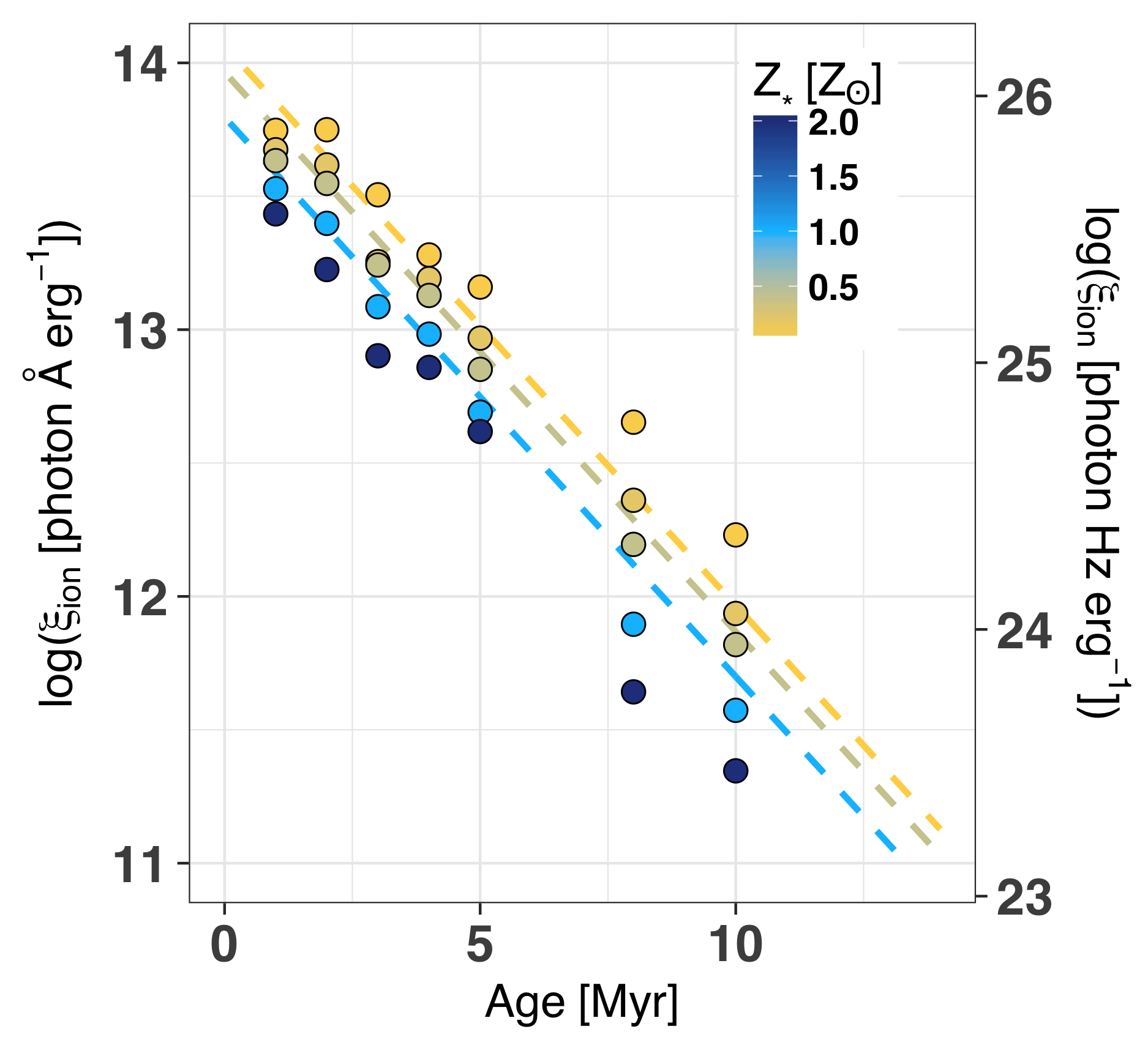
Throughout this paper we have described the ionizing continua using F900/F1500, a measure of the ionizing continuum at a single wavelength. However, the principle goal of this paper is to use the FUV stellar continua to determine a more physically important parameter: the total number of ionizing photons produced by massive star populations (). scales linearly with the star formation rate, such that populations forming more stars generate more ionizing photons (Madau et al., 1998; Kennicutt, 1998; Kennicutt & Evans, 2012; Madau & Dickinson, 2014). Therefore, the ionizing photon production efficiency, , compares the capacity of different stellar populations to produce ionizing photons at a given FUV luminosity. The ionizing photon production efficiency is defined from the stellar models as
| (8) |
or in the more common units as
| (9) |
When multiplied by the reddening corrected FUV luminosity, L1500, determines the total number of ionizing photons generated by a stellar population.
Figure 21 shows that the stellar population parameters, particular stellar age, determine . A 2 Myr, 0.4 Z⊙ starburst99 stellar population produces 50 times more ionizing photons per L1500 than a similar 10 Myr population. Similarly, a 0.05 Z⊙, 2 Myr population produces 3 times more ionizing photons than a 2 Z⊙ population of the same age. These numbers stress the relative importance of age for the production of ionizing photons. The multivariate relationship between and the starburst99 stellar population properties is
| (10) |
or
| (11) |
This relation powerfully illustrates that the total number of ionizing photons, , can be determined from the stellar population age, metallicity, and the extinction-corrected L1500. As with the F900/F1500 relations, the models vary from the fitted relation at a given age (the curves in Figure 21 are single metallicity relations), but Equation 10 and Equation 11 characterize the overall evolution of the efficiency of ionizing photon production with an observed stellar age and metallicity.
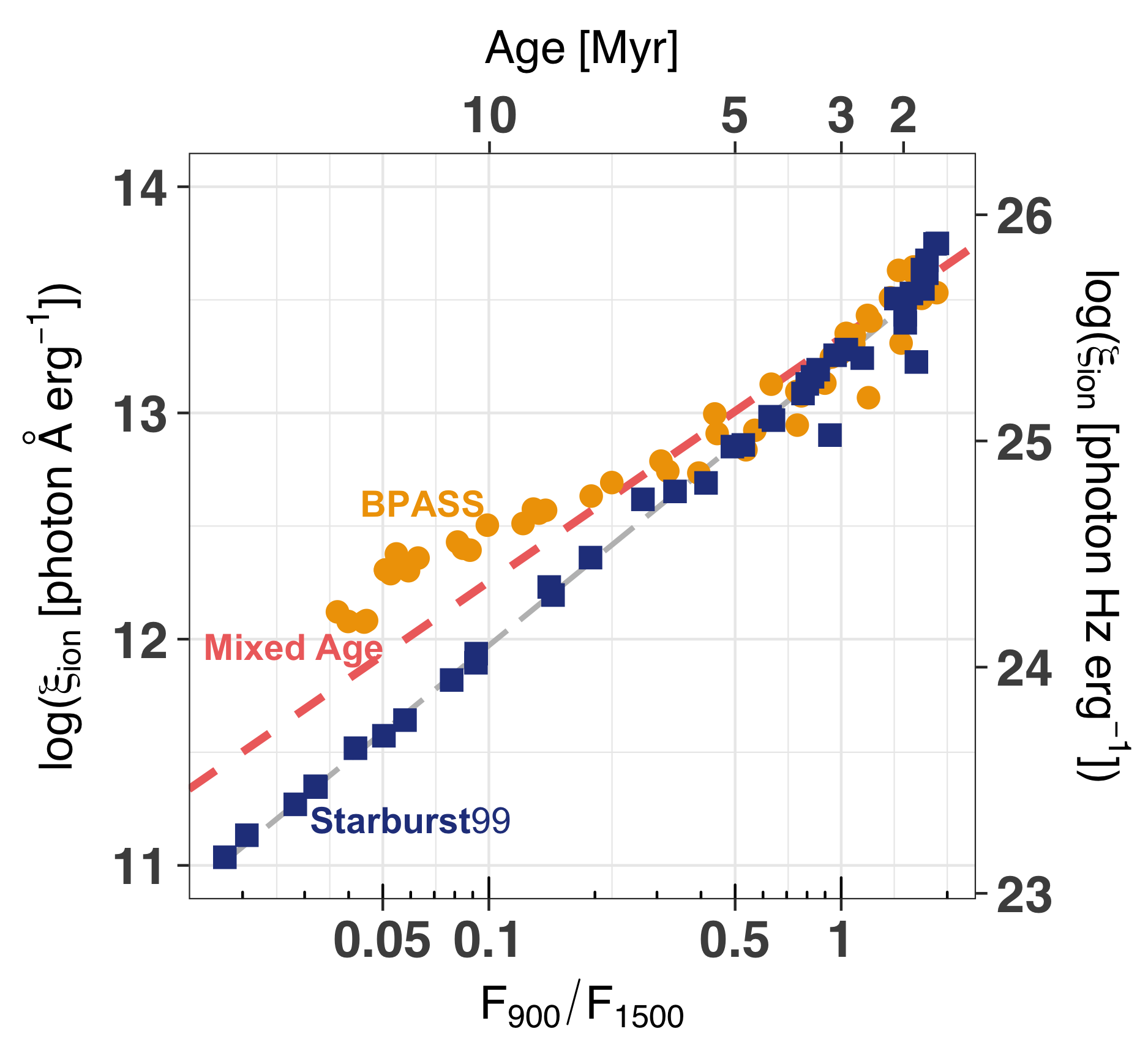
Equation 10 & 11 have exceptionally similar scalings with age and Z∗ as F900/F1500 does in Figure 15. In fact, F900/F1500 strongly scales with (Figure 22) as
| (12) |
The strong relationship between F900/F1500 and may come as a surprise, but it is simply related by changes in stellar temperature. As the stellar temperature decreases with increasing stellar age, the hydrogen within the stellar atmospheres becomes more neutral and the stellar Lyman break increases (compare the 2 Myr to 3 and 5 Myr models in Figure 12). Thus, F900/F1500 effectively measures the hydrogen ionization fraction within the stellar atmosphere, which is related to the stellar temperature by both the stellar age and metallicity. Since stars are to first order complicated black bodies, it follows that the integrated ionizing energy emitted by massive stars, , must strongly scale with the stellar temperature (or proxies thereof, such as F900/F1500) through the Stephan-Boltzmann law. Thus, the analysis of the variation of F900/F1500 with age and Z∗ from Section 5.2.1 directly extends to .
Populations with binary evolution produce a flatter relationship between and F900/F1500 (orange circles in Figure 22), because binary populations produce more evolved stars, which in turn have higher temperatures at older ages. from bpass models scales as
| (13) |
At F900/F1500 = (or an age of 10 Myr), populations with binary evolution produce three times more total ionizing photons than populations without binary evolution. However, at ages Myr both models produce a similar number of ionizing photons. Thus, binary evolution increases the total number of ionizing photons produced by older stellar populations, but has minimal impact on the youngest, 2-4 Myr stellar populations.
Similarly, mixed age stellar populations produce more ionizing photons per L1500 at older light-weighted ages than a single burst star formation history (red line in Figure 22), due to the outsized contribution of younger populations (Section 5.3). Using the same MCMC sample as Section 5.2.2, there is a strong correlation between and F900/F1500 for the mixed age starburst99 population:
| (14) |
These three cases illustrate that at older light-weighted ages strongly depends on both the star formation history and impact of binary evolution.
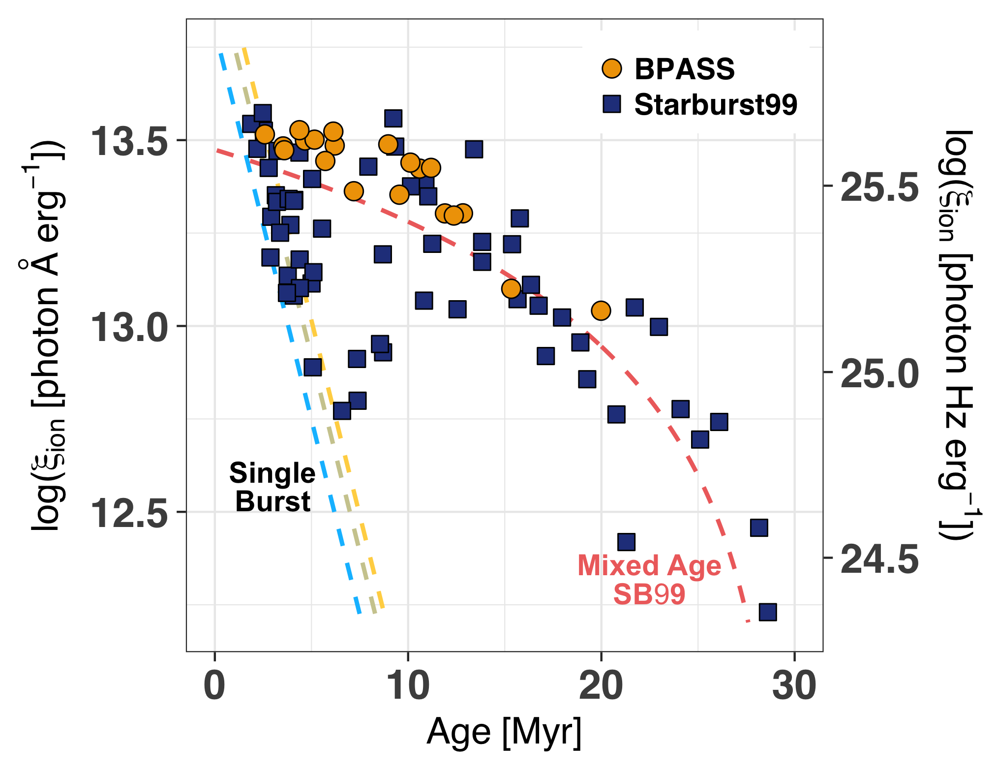
Finally, we compare the ionizing photon production efficiencies of the observed stellar spectra in Figure 23. The values are determined by integrating the entire ionizing continuum, divided by the photon energy, of the FUV stellar continuum fits. Galaxies that we defined as having a single burst star formation history in Section 5.2.2 closely track the single burst relations of Equation 10 (blue, tan, and yellow curves), while mixed age populations follow the curve defined by the synthetic MCMC population (red curve).
The median log([Å erg-1]) of the observed sample and the starburst99 models is ( for log([Hz erg-1])) and the full log([Å erg-1]) range is 12.2–13.6 (24.4–25.7 for log([Hz erg-1])). The galaxies within our sample have over an order of magnitude range in the number of ionizing photons that high-mass stars produce per FUV luminosity. strongly varies from galaxy-to-galaxy; accurate stellar continuum modeling must determine how efficiently ionizing photons are produced. Perhaps most importantly, the range of inferred shows that the number of ionizing photons cannot be estimated from the observed FUV luminosity to better than an order of magnitude without estimating the stellar population age and metallicity.
The measured values are largely consistent with values inferred in the literature. Kennicutt & Evans (2012) used a constant star formation history, 1 Z⊙ starburst99 model to derive expressions for the star formation rate of normal local galaxies. These models have log([Å erg-1]) = 13.0 (log([Hz erg-1]) = 25.1), which is statistically consistent with the median value of our sample. While this assumed value agrees with the median of our sample, it will not agree on a galaxy-by-galaxy basis, to which a detailed analysis of the massive star properties is required. At higher redshifts, it is typically presumed that more extreme objects, with log([Hz erg-1]), are required to reionize the early universe if 20% of their ionizing photons escape the interstellar medium (Robertson et al., 2013; Bouwens et al., 2016; Finkelstein et al., 2019). Half of our sample, 31 of 61 (51%), have greater than the value typically assumed for cosmic reionization (log([Hz erg-1])). This is not surprising because the galaxies were selected to be bright in the rest-frame FUV, such that the stars must be relatively young. Finally, local galaxies that have been observed to emit ionizing photons also have very young stellar populations (Izotov et al., 2018) and correspondingly extreme values of [Hz erg-1] = 25.6 measured from their C III] 1909Å emission lines (Schaerer et al., 2018). These values are consistent with the youngest 2–3 Myr stellar populations in both of our samples.
The bpass fits to the MegaSaura spectra indicate that binary evolution increases the duration of the peak , but not the peak itself (orange circles versus blue squares in Figure 23). At the youngest ages, the inferred from the starburst99 and bpass fits are very similar; binary evolution does not increase the maximum inferred . Consequently, the youngest stellar populations, which produce the majority of the ionizing photons, have consistent values regardless of the chosen binary evolution model. Thus, binary evolution does not increase the maximum , rather it elongates the period which stellar populations produce their maximum . If binary evolution is important at high redshifts, it would increase the total number of ionizing photons that high-mass stellar populations produced over their entire lifetimes, and make it easier for stars to reionize the universe.
A surprising prediction from the bpass models in Figure 23 is that the values of 4-7 Myr populations do not decrease along the single burst tracks of Figure 21. Rather, the WR-stars in populations with binary evolution keep the elevated, and nearly constant at the maximum value, over the 10 Myr lifetime of O-stars. Comparing the inferred ionizing continua of RCS Knot E and S0108+0624 in Figure 16 demonstrates this behavior: the two galaxies have substantially different light-weighted ages but similar bpass ionizing continua. Thus, the number of ionizing photons produced by a stellar population with binary evolution does not vary until the stellar population is older than 10 Myr. As mentioned above, this could substantially increase the total number of ionizing photons generated over the integrated lifetime of stellar populations within the epoch of reionization. This is also a testable observation of the impact of binary evolution using the nebular emission lines.
Determining the total number of ionizing photons intrinsically produced by a given stellar population is a key strength of FUV spectral synthesis. This analysis infers the total number of ionizing photons, as well as their spectral distribution, using observable spectral features from the same massive stars that emit the ionizing photons. In theory, spectral synthesis promises to be an extremely powerful tool for a wide assortment of extragalactic applications, from understanding the generation of nebular emission lines to uncovering the sources of cosmic reionization. In practice, determining the total number of ionizing photons requires precise constraints on the stellar population age, metallicity, star formation history, and the impact of binary star evolution (Figure 21 and Figure 22). We demonstrated throughout this paper that massive star spectral features constrain the age, metallicity, and star formation history. However, we also emphasized that the non-ionizing FUV stellar continuum alone cannot constrain the impact of binary evolution. Binary evolution does not dramatically impact the number of ionizing photons produced per FUV luminosity of the youngest stellar populations (¡4 Myr), but it significantly increases the number of ionizing photons produced by older populations. Without constraining the impact of binary evolution, there is up to a factor of 7 uncertainty in the total number of ionizing photons produced by older stellar populations.
6 Summary
We have studied the massive star populations in a sample of 61 star-forming galaxies comprised of 42 at from the HST archive and 19 at from the MegaSaura sample. We fit a simple linear combination of single age, fully theoretical stellar models to the far-ultraviolet stellar continuum (Å). From these fits we derived light-weighted ages and metallicities of the stellar populations, and extrapolated the fits to infer their ionizing continua (Å).
Individual, stellar spectral features agree with the inferred light-weighted properties. The C IV stellar wind line varies with the inferred stellar age and metallicity in different and distinguishable ways (Figure 3), such that the C IV emission depends on stellar age (Figure 4) and the absorption depends on metallicity (Figure 5). The N V line strongly depends on age and is nearly independent of metallicity (Figure 6). Very young stellar populations have broad ( km s-1) He II emission from Wolf-Rayet stars, while older populations have negligible He II features (Figure 8). Finally, old populations have C III and Si III photospheric absorption features, while these features are undetected in younger populations (Figure 9).
The light-weighted stellar metallicity is strongly correlated with (), and consistent with, the nebular metallicity (Figure 11). The metallicity relationship does not depend on redshift, as we find stars and gas to have similar metallicities. Stellar metallicities may be the most reliable, yet time-consuming, method to infer metallicities at high redshift (Section 5.1).
We used the stellar continuum models to demonstrate how the stellar ionizing continuum depends on stellar population properties (Section 5.2). Specifically, we characterized the ionizing continuum using three ratios of the ionizing flux density at different wavelengths to the non-ionizing flux density at 1500Å. We focused on how the flux density ratio at 900Å to 1500Å, or F900/F1500, depends on stellar population properties, because 900Å is the most common wavelength to observe the ionizing continuum. Theoretical stellar models demonstrate that the strength and spectral shape of the ionizing continuum of a single burst strongly depends on the stellar age (Figure 12 and Figure 13) and metallicity (Figure 14). A multivariate relationship between F900/F1500 and both the age and metallicity (Equation 5) describes most of the variation in F900/F1500 for a single burst of star formation (Figure 15).
We then inferred the ionizing continuum of the observed stellar populations by extrapolating the fits to the observed stellar continua. Stellar populations with older light-weighted ages have weaker inferred ionizing continua (Figure 16). However, only half (31 of 61) of the sample follows the single burst F900/F1500 relations (Figure 17). The other half of the sample has a mixture of stellar populations at multiple ages. The mixed age populations have stronger inferred ionizing continua at older ages than prescribed by a single burst model. The inferred F900/F1500 of these galaxies is strongly linearly anti-correlated (5.5) with the light-weighted age (Equation 6). These two populations are split at a light-weighted age of 8.6 Myr.
Mixed age populations have stronger ionizing continua than single bursts of a similar age due to the presence of very young stellar populations (Figure 17). We emphasized the differences between mixed age populations and the typically assumed continuous star formation history (Section 5.3). Chiefly, the mixed age continua depend on the relative mixture of age and metallicity. Thus, age sensitive spectral features (C IV, N V, and He II) can vary, and the ionizing continuum can correspondingly increase or decrease. Mixed age stellar populations produce significantly more ionizing photons than both a single burst with the same light-weighted age and a continuous star formation history, while having the same metallicity as the nebular gas (Figure 20). This is in stark contrast with previous work that assume a constant star formation history and we emphasized that the only difference is the assumed star formation history.
Our fiducial stellar models are single star starburst99 models mainly because these provided sufficient spectral resolution at all wavelengths (see the discussion in Section 3.2.2). We also fit the MegaSaura sample with stellar models that include binary evolution (bpass models), but do not find significant differences between the starburst99 and bpass fits to the FUV features (compare the blue and gold lines in Figure 3–6). Similarly, the light-weighted metallicities and ages are similar, as long as we only consider young ages for which the bpass spectral resolution is adequate (Figure 18). The most significant difference is that bpass models produce up to 12 times more high-energy ionizing photons than starburst99 models at older ages and lower metallicities (Figure 15 and Figure 16). Consequently, the number of ionizing photons produced by a stellar population depends on the observationally unconstrained impact of binary evolution.
We provide scaling relations for the total number of ionizing photons produced per FUV luminosity (). strongly depends on the age, metallicity, star formation history, and presence of binary stars (Figure 21 and Figure 22). The inferred values from our observations have an order of magnitude scatter that strongly depends on stellar population properties (Figure 23). We emphasize that times the extinction corrected FUV luminosity determines the total number of ionizing photons produced by a stellar population. While fitting the FUV stellar continuum promises to be a powerful tool in determining the total number of ionizing photons produced by high-mass stars, without constraining the impact of binary evolution there is a factor of 7 uncertainty in the total number of ionizing photons produced by older stellar populations.
The rest-frame FUV spectral features of massive stars mirror the production of ionizing photons. Stellar population synthesis can estimate many properties required to infer the number of ionizing photons produced by stars and determine the source of cosmic reionization. This type of modeling is currently infeasible for galaxies within the epoch of reioniziation, but observations of the stellar continuum will be possible with future 30 m class telescopes and the James Webb Space Telescope. Stellar population synthesis of the most massive stars, as presented here, will be the most direct method to constrain the number of ionizing photons produced by the most distant star-forming galaxies.
| (1) | (2) | (3) | (4) | (5) | (6) | (7) | (8) | (9) | (10) | (11) |
|---|---|---|---|---|---|---|---|---|---|---|
| Galaxy name | E(B-V) | E(B-V) | Z | Z∗ | Z∗ | Age | Age | F900/F1500 | Spectral | |
| SB99 | BPASS | SB99 | BPASS | SB99 | BPASS | SB99 | Reference | |||
| [mag] | [mag] | [Z⊙] | [Z⊙] | [Z⊙] | [Myr] | [Myr] | ||||
| RCS-0327-1326 Knot E | 1.7034 | 0.31 | 0.29 | 0.34c | 0.24 0.03 | 0.18 0.02 | 2.54 0.14 | 2.59 0.14 | 1.55 0.08 | 3, 13, 10 |
| Sunburst Arc Region 5 | 2.3709 | 0.15 | 0.15 | – | 0.55 0.04 | 0.66 0.05 | 2.92 0.08 | 3.59 0.09 | 1.14 0.05 | 4, 11 |
| S003341.5+024217 | 2.3887 | 0.33 | 0.32 | – | 0.84 0.04 | 0.74 0.03 | 5.00 0.51 | 3.53 0.36 | 0.76 0.08 | 10 |
| RCS-0327-1326 Knot U | 1.7039 | 0.27 | 0.28 | 0.34c | 0.29 0.07 | 0.09 0.02 | 5.03 1.44 | 5.16 1.47 | 1.07 0.31 | 3, 10, 13 |
| S095738.7+050929 | 1.8204 | 0.17 | 0.17 | – | 0.17 0.05 | 0.20 0.06 | 7.36 1.64 | 4.38 0.98 | 0.52 0.20 | 1, 10 |
| S090003.3+223408 | 2.0326 | 0.10 | 0.09 | 0.31a | 0.38 0.02 | 0.30 0.02 | 7.39 0.41 | 7.19 0.39 | 0.39 0.03 | 5, 10 |
| SPT0356 | 2.362 | 0.14 | 0.14 | – | 0.220.07 | 0.160.05 | 8.553.88 | 5.712.59 | 0.470.33 | – |
| S010842.2+062444 | 1.9102 | 0.18 | 0.20 | – | 0.50 0.03 | 0.35 0.02 | 8.71 1.06 | 6.20 0.75 | 0.53 0.09 | 9, 10 |
| SPT2325 | 1.5799 | 0.17 | 0.17 | – | 0.27 0.03 | 0.15 0.02 | 9.24 2.42 | 6.13 1.61 | 1.36 0.54 | – |
| Cosmic Horseshoe | 2.3812 | 0.11 | 0.09 | 0.57b | 0.52 0.07 | 0.20 0.03 | 9.33 4.20 | 11.91 5.35 | 1.13 0.76 | 2, 10 |
| SPT0142 | 2.674 | 0.19 | 0.17 | – | 0.230.04 | 0.140.03 | 10.153.73 | 12.364.54 | 1.060.65 | – |
| RCS-0327-1326 Knot G | 1.7039 | 0.24 | 0.24 | 0.34c | 0.29 0.04 | 0.24 0.04 | 10.90 1.77 | 4.66 0.76 | 0.97 0.34 | 3, 10, 13 |
| S000451.7-010321 | 1.6811 | 0.33 | 0.30 | 0.25d | 0.25 0.02 | 0.15 0.01 | 13.41 0.80 | 10.60 0.63 | 1.08 0.22 | 9, 10 |
| S142954.9+120239 | 2.8245 | 0.18 | 0.20 | – | 0.64 0.05 | 0.60 0.04 | 15.38 2.68 | 9.55 1.66 | 0.68 0.30 | 8, 10 |
| SPT0310 | 1.9960 | 0.27 | 0.29 | – | 0.23 0.04 | 0.30 0.05 | 15.66 2.87 | 8.97 1.65 | 0.67 0.37 | – |
| PSZ0441 | 1.8008 | 0.30 | 0.30 | – | 0.10 0.05 | 0.39 0.18 | 19.27 4.47 | 11.19 2.59 | 0.41 0.57 | – |
| S152745.1+065219 | 2.7623 | 0.33 | 0.32 | ¡0.65f | 0.49 0.04 | 0.36 0.03 | 21.30 3.32 | 12.84 2.00 | 0.22 0.12 | 6, 10 |
| S122651.3+215220 | 2.9260 | 0.13 | 0.13 | – | 0.34 0.02 | 0.14 0.01 | 26.10 1.29 | 19.98 0.99 | 0.31 0.09 | 7, 10 |
| Cosmic Eye | 3.0735 | 0.38 | 0.36 | 0.81e | 0.65 0.02 | 0.50 0.02 | 28.62 0.80 | 15.34 0.43 | 0.15 0.03 | 10, 12 |
| (1) | (2) | (3) | (4) | (5) | (6) | (7) | (8) | (9) | (10) | (11) |
|---|---|---|---|---|---|---|---|---|---|---|
| Galaxy name | E(B-V) | Z | Z∗ | Age | F900/F1500 | PID | Z | Metallicity | Spectra | |
| [mag] | [Z⊙] | [Z⊙] | [Myr] | Ref | Calibration | Ref | ||||
| J1416+1223 | 0.1231 | 0.14 | 0.60 | 0.600.05 | 1.88 0.35 | 1.360.28 | 13017 | Heckman et al. (2015) | PP04 | 1 6 |
| J0150+1260 | 0.1467 | 0.12 | 0.50 | 0.520.13 | 2.20 2.17 | 1.231.25 | 11727 | Heckman et al. (2015) | PP04 | 1 6 |
| J0824+2806 | 0.0472 | 0.28 | 0.35 | 0.550.08 | 2.483.12 | 1.490.88 | 13017 | Heckman et al. (2015) | PP04 | 1 6 |
| J0907+5327 | 0.0299 | 0.08 | 0.22 | 0.560.19 | 2.79 1.31 | 1.230.72 | 12583 | Östlin et al. (2014) | Direct | 5 9 10 |
| NGC 7552 | 0.0054 | 0.71 | 1.12 | 0.990.05 | 2.88 0.04 | 1.160.07 | 12173 | Moustakas et al. (2011) | KK04 | 8 |
| J0055-0021 | 0.1674 | 0.25 | 0.39 | 0.420.15 | 3.16 2.27 | 1.200.97 | 11727 | Heckman et al. (2015) | PP04 | 1 6 |
| J1429+0643 | 0.1736 | 0.20 | 0.27 | 0.360.09 | 3.21 0.36 | 1.110.30 | 13017 | Heckman et al. (2015) | PP04 | 1 6 |
| J0926+4427 | 0.1807 | 0.00 | 0.14 | 0.160.06 | 3.24 0.37 | 1.310.49 | 11727 | Heckman et al. (2015) | PP04 | 1 6 |
| J0808+3948 | 0.0912 | 0.15 | 1.12 | 1.460.04 | 3.380.07 | 0.910.02 | 11727 | Heckman et al. (2015) | PP04 | 1 6 |
| J0921+4509 | 0.2350 | 0.19 | 0.95 | 1.030.15 | 3.730.62 | 0.770.13 | 11727 | Heckman et al. (2015) | PP04 | 1 2 6 |
| NGC 6090 | 0.0293 | 0.22 | 0.51 | 0.760.03 | 3.77 0.11 | 0.830.04 | 12173 | Cortijo-Ferrero et al. (2017) | M13 | 8 |
| J0021+0052 | 0.0984 | 0.10 | 0.32 | 0.450.13 | 3.821.28 | 1.060.30 | 13017 | Heckman et al. (2015) | PP04 | 1 6 |
| J1415+0540 | 0.0819 | 0.13 | 0.39 | 0.340.10 | 3.91 2.40 | 1.010.69 | 13017 | Heckman et al. (2015) | PP04 | 1 6 |
| NGC 3256 | 0.0094 | 0.49 | 1.10 | 0.570.12 | 4.08 1.45 | 0.760.31 | 12173 | Engelbracht et al. (2008) | PP04 | 8 |
| J0213+1259 | 0.2190 | 0.40 | 1.12 | 1.080.22 | 4.091.65 | 0.910.33 | 13017 | Heckman et al. (2015) | PP04 | 1 6 |
| KISSR 1578 | 0.0279 | 0.11 | 0.24 | 0.480.06 | 4.11 2.03 | 1.050.54 | 11522 | Östlin et al. (2014) | Direct | 11 |
| J1112+5503 | 0.1315 | 0.25 | 0.68 | 0.650.09 | 4.38 3.54 | 1.150.94 | 13017 | Heckman et al. (2015) | PP04 | 1 6 |
| NGC 4214 | 0.0010 | 0.30 | 0.32 | 0.330.06 | 4.39 0.30 | 0.950.20 | 11579 | Kobulnicky & Skillman (1996) | Direct | 7 |
| J1315+6207 | 0.0308 | 0.43 | 1.02 | 0.970.17 | 4.40 2.23 | 0.750.40 | 12583 | This work | Direct | 5 9 10 |
| NGC 7714 | 0.0093 | 0.42 | 0.60 | 0.840.02 | 5.07 0.06 | 0.510.01 | 12604 | Gonzalez-Delgado et al. (1995) | Direct | 3 |
| SBS 1415+437 | 0.0020 | 0.14 | 0.08 | 0.080.02 | 5.10 0.21 | 0.810.19 | 11579 | Thuan et al. (1999) | Direct | 7 |
| KISSR 218 | 0.0209 | 0.46 | 1.51 | 1.200.19 | 5.55 3.73 | 1.030.71 | 11522 | Salzer et al. (2005) | EP84 | 11 |
| J1429+1653 | 0.1816 | 0.19 | 0.42 | 0.400.07 | 6.58 2.73 | 0.420.19 | 13017 | Heckman et al. (2015) | PP04 | 1 6 |
| J0938+5428 | 0.1021 | 0.11 | 0.21 | 0.240.08 | 7.94 3.34 | 1.070.58 | 11727 | Heckman et al. (2015) | PP04 | 1 6 |
| J1025+3622 | 0.1265 | 0.11 | 0.26 | 0.180.05 | 8.69 3.64 | 0.830.43 | 13017 | Heckman et al. (2015) | PP04 | 1 6 |
| KISSR 182 | 0.0224 | 0.32 | 0.45 | 0.530.17 | 10.82 4.58 | 0.710.38 | 12027 | Salzer et al. (2005) | EP84 | 11 |
| J1525+0757 | 0.0757 | 0.14 | 0.59 | 0.530.09 | 11.04 5.18 | 0.970.48 | 13017 | Heckman et al. (2015) | PP04 | 1 6 |
| Shoc 22 | 0.0179 | 0.10 | 0.23 | 0.280.05 | 11.25 2.97 | 0.740.23 | 15099 | This work | Direct | – |
| J1250+0734 | 0.0382 | 0.19 | 0.66 | 0.690.17 | 13.83 6.80 | 0.810.44 | 12583 | Östlin et al. (2014) | Direct | 5 9 10 |
| MRK 1486 | 0.0338 | 0.12 | 0.13 | 0.100.05 | 13.83 2.58 | 0.790.46 | 12583 | Östlin et al. (2014) | Direct | 5 9 10 |
| Haro 11 | 0.0206 | 0.09 | 0.40 | 0.380.02 | 15.78 1.48 | 0.770.08 | 13017 | James et al. (2013) | Direct | 1 6 |
| SBS 0926+606A | 0.0137 | 0.14 | 0.21 | 0.320.08 | 16.36 4.83 | 0.720.28 | 15099 | Berg et al. (2016) | Direct | – |
| J1307+5427 | 0.0325 | 0.37 | 0.30 | 0.830.14 | 16.75 4.87 | 0.630.21 | 12583 | This work | Direct | 5 9 10 |
| NGC 5253_1 | 0.0014 | 0.34 | 0.30 | 0.310.04 | 17.13 2.43 | 0.530.10 | 11579 | Walsh & Roy (1989) | Direct | 7 |
| KISSR 108 | 0.0236 | 0.19 | 0.30 | 0.250.14 | 17.96 5.12 | 0.560.36 | 12027 | Salzer et al. (2005) | EP84 | 11 |
| J1144+4012 | 0.1270 | 0.26 | 0.51 | 0.410.10 | 18.91 5.71 | 0.510.20 | 13017 | Heckman et al. (2015) | PP04 | 1 6 |
| 1 Zw 18 | 0.0025 | 0.12 | 0.03 | 0.050.01 | 20.78 0.71 | 0.350.07 | 11579 | Izotov et al. (1997) | Direct | 7 |
| KISSR 242 | 0.0378 | 0.22 | 0.49 | 0.510.13 | 21.73 5.16 | 0.560.20 | 11522 | Salzer et al. (2005) | EP84 | 4 11 |
| IRAS 08339 | 0.0191 | 0.23 | 0.58 | 0.520.03 | 22.98 1.22 | 0.460.04 | 12173 | López-Sánchez et al. (2006) | D02 | 8 |
| NGC 4670 | 0.0036 | 0.26 | 0.32 | 0.370.04 | 24.10 1.49 | 0.410.05 | 11579 | Heckman et al. (1998) | Direct | 7 |
| NGC 4449 | 0.0007 | 0.37 | 0.42 | 0.410.03 | 25.11 1.47 | 0.330.03 | 11579 | Marble et al. (2010) | Direct | 7 |
| NGC 3690 | 0.0102 | 0.21 | 0.74 | 0.810.10 | 28.16 1.07 | 0.120.01 | 11579 | Heckman et al. (1998) | Direct | 7 |
| (1) | (2) | (3) |
|---|---|---|
| Galaxy name | log() SB99 | log() BPASS |
| log([photon Å erg-1]) | log([photon Å erg-1]) | |
| RCS-0327-1326 Knot E | 13.530.03 | 13.520.03 |
| Sunburst Arc Region 5 | 13.290.02 | 13.470.02 |
| S003341.5+024217 | 13.110.05 | 13.480.05 |
| RCS-0327-1326 Knot U | 13.400.16 | 13.500.16 |
| S095738.7+050929 | 12.910.20 | 13.530.21 |
| S090003.3+223408 | 12.800.05 | 13.360.05 |
| SPT0356 | 12.950.37 | 13.440.38 |
| S010842.2+062444 | 12.930.09 | 13.490.10 |
| SPT2325 | 13.560.21 | 13.52 0.21 |
| Cosmic Horseshoe | 13.48 0.36 | 13.30 0.35 |
| SPT0142 | 13.38 0.33 | 13.30 0.33 |
| RCS-0327-1326 Knot G | 13.38 0.19 | 13.50 0.19 |
| S000451.7-010321 | 13.48 0.11 | 13.42 0.11 |
| S142954.9+120239 | 13.22 0.23 | 13.35 0.24 |
| SPT0310 | 13.07 0.29 | 13.49 0.30 |
| PSZ0441 | 12.86 0.75 | 13.43 0.79 |
| S152745.1+065219 | 12.42 0.29 | 13.30 0.31 |
| S122651.3+215220 | 12.74 0.16 | 13.04 0.16 |
| Cosmic Eye | 12.23 0.10 | 13.10 0.11 |
| (1) | (2) |
|---|---|
| Galaxy name | log() |
| log([photon Å erg-1]) | |
| J1416+1223 | 13.540.11 |
| J0150+1260 | 13.480.54 |
| J0824+2806 | 13.570.32 |
| J0907+5327 | 13.430.31 |
| NGC 7552 | 13.180.03 |
| J0055-0021 | 13.350.43 |
| J1429+0643 | 13.330.14 |
| J0926+4427 | 13.470.20 |
| J0808+3948 | 13.250.01 |
| J0921+4509 | 13.090.09 |
| NGC 6090 | 13.140.03 |
| J0021+0052 | 13.340.15 |
| J1415+0540 | 13.270.36 |
| NGC 3256 | 13.080.22 |
| J0213+1259 | 13.340.19 |
| KISSR 1578 | 13.340.27 |
| J1112+5503 | 13.470.44 |
| NGC 4214 | 13.180.11 |
| J1315+6207 | 13.100.29 |
| NGC 7714 | 12.890.01 |
| SBS 1415+437 | 13.140.13 |
| KISSR 218 | 13.260.37 |
| J1429+1653 | 12.770.24 |
| J0938+5428 | 13.430.29 |
| J1025+3622 | 13.190.27 |
| KISSR 182 | 13.070.28 |
| J1525+0757 | 13.350.27 |
| Shoc 22 | 13.220.17 |
| J1250+0734 | 13.230.29 |
| MRK 1486 | 13.170.31 |
| Haro 11 | 13.290.06 |
| SBS 0926+606A | 13.110.21 |
| J1307+5427 | 13.050.18 |
| NGC 5253_1 | 12.920.10 |
| KISSR 108 | 13.020.34 |
| J1144+4012 | 12.960.20 |
| 1 Zw 18 | 12.760.11 |
| KISSR 242 | 13.050.19 |
| IRAS 08339 | 13.000.05 |
| NGC 4670 | 12.780.07 |
| NGC 4449 | 12.690.05 |
| NGC 3690 | 12.460.07 |
References
- Abbott & Conti (1987) Abbott D. C., Conti P. S., 1987, ARA&A, 25, 113
- Alam et al. (2015) Alam S., et al., 2015, ApJS, 219, 12
- Alexandroff et al. (2015) Alexandroff R. M., Heckman T. M., Borthakur S., Overzier R., Leitherer C., 2015, ApJ, 810, 104
- Asplund et al. (2009) Asplund M., Grevesse N., Sauval A. J., Scott P., 2009, ARA&A, 47, 481
- Baldwin et al. (1981) Baldwin J. A., Phillips M. M., Terlevich R., 1981, PASP, 93, 5
- Baldwin et al. (1991) Baldwin J. A., Ferland G. J., Martin P. G., Corbin M. R., Cota S. A., Peterson B. M., Slettebak A., 1991, ApJ, 374, 580
- Bayliss et al. (2011) Bayliss M. B., Gladders M. D., Oguri M., Hennawi J. F., Sharon K., Koester B. P., Dahle H., 2011, ApJ, 727, L26
- Belokurov et al. (2007) Belokurov V., et al., 2007, ApJ, 671, L9
- Berg et al. (2016) Berg D. A., Skillman E. D., Henry R. B. C., Erb D. K., Carigi L., 2016, ApJ, 827, 126
- Berg et al. (2018) Berg D. A., Erb D. K., Auger M. W., Pettini M., Brammer G. B., 2018, ApJ, 859, 164
- Berg et al. (2019) Berg D. A., Erb D. K., Henry R. B. C., Skillman E. D., McQuinn K. B. W., 2019, arXiv e-prints,
- Bian et al. (2010) Bian F., et al., 2010, ApJ, 725, 1877
- Bordoloi et al. (2016) Bordoloi R., Rigby J. R., Tumlinson J., Bayliss M. B., Sharon K., Gladders M. G., Wuyts E., 2016, MNRAS, 458, 1891
- Borthakur et al. (2014) Borthakur S., Heckman T. M., Leitherer C., Overzier R. A., 2014, Science, 346, 216
- Bouret et al. (2003) Bouret J.-C., Lanz T., Hillier D. J., Heap S. R., Hubeny I., Lennon D. J., Smith L. J., Evans C. J., 2003, ApJ, 595, 1182
- Bouwens et al. (2016) Bouwens R. J., et al., 2016, ApJ, 833, 72
- Brinchmann et al. (2004) Brinchmann J., Charlot S., Heckman T. M., Kauffmann G., Tremonti C., White S. D. M., 2004, ArXiv Astrophysics e-prints,
- Bruzual & Charlot (2003) Bruzual G., Charlot S., 2003, MNRAS, 344, 1000
- Byler et al. (2018) Byler N., Dalcanton J. J., Conroy C., Johnson B. D., Levesque E. M., Berg D. A., 2018, ApJ, 863, 14
- Calzetti et al. (2000) Calzetti D., Armus L., Bohlin R. C., Kinney A. L., Koornneef J., Storchi-Bergmann T., 2000, ApJ, 533, 682
- Cardelli et al. (1989) Cardelli J. A., Clayton G. C., Mathis J. S., 1989, ApJ, 345, 245
- Castor et al. (1975) Castor J. I., Abbott D. C., Klein R. I., 1975, ApJ, 195, 157
- Chabrier (2003) Chabrier G., 2003, PASP, 115, 763
- Chisholm et al. (2016) Chisholm J., Tremonti C. A., Leitherer C., Chen Y., Wofford A., 2016, MNRAS, 457, 3133
- Choi et al. (2017) Choi J., Conroy C., Byler N., 2017, ApJ, 838, 159
- Conroy (2013) Conroy C., 2013, ARA&A, 51, 393
- Conroy & van Dokkum (2012) Conroy C., van Dokkum P., 2012, ApJ, 747, 69
- Conroy et al. (2014) Conroy C., Graves G. J., van Dokkum P. G., 2014, ApJ, 780, 33
- Cortijo-Ferrero et al. (2017) Cortijo-Ferrero C., et al., 2017, MNRAS, 467, 3898
- Crowther (2007) Crowther P. A., 2007, ARA&A, 45, 177
- Dahle et al. (2016) Dahle H., et al., 2016, A&A, 590, L4
- Denicoló et al. (2002) Denicoló G., Terlevich R., Terlevich E., 2002, MNRAS, 330, 69
- Diehl et al. (2009) Diehl H. T., et al., 2009, ApJ, 707, 686
- Drew (1989) Drew J. E., 1989, ApJS, 71, 267
- Edmunds & Pagel (1984) Edmunds M. G., Pagel B. E. J., 1984, MNRAS, 211, 507
- Elbaz et al. (2007) Elbaz D., et al., 2007, A&A, 468, 33
- Eldridge & Stanway (2009) Eldridge J. J., Stanway E. R., 2009, MNRAS, 400, 1019
- Eldridge et al. (2017) Eldridge J. J., Stanway E. R., Xiao L., McClelland L. A. S., Taylor G., Ng M., Greis S. M. L., Bray J. C., 2017, Publications of the Astron. Soc. of Australia, 34, e058
- Engelbracht et al. (2008) Engelbracht C. W., Rieke G. H., Gordon K. D., Smith J.-D. T., Werner M. W., Moustakas J., Willmer C. N. A., Vanzi L., 2008, ApJ, 678, 804
- Ferland et al. (2013) Ferland G. J., et al., 2013, rmxaa, 49, 137
- Finkelstein et al. (2019) Finkelstein S. L., et al., 2019, arXiv e-prints,
- Fox et al. (2013) Fox A. J., Richter P., Wakker B. P., Lehner N., Howk J. C., Ben Bekhti N., Bland-Hawthorn J., Lucas S., 2013, ApJ, 772, 110
- Fragos et al. (2013) Fragos T., Lehmer B. D., Naoz S., Zezas A., Basu-Zych A., 2013, ApJ, 776, L31
- France et al. (2010) France K., Nell N., Green J. C., Leitherer C., 2010, ApJ, 722, L80
- Georgy et al. (2012) Georgy C., Ekström S., Meynet G., Massey P., Levesque E. M., Hirschi R., Eggenberger P., Maeder A., 2012, A&A, 542, A29
- Gladders & Yee (2005) Gladders M. D., Yee H. K. C., 2005, ApJS, 157, 1
- Gonzalez-Delgado et al. (1995) Gonzalez-Delgado R. M., Perez E., Diaz A. I., Garcia-Vargas M. L., Terlevich E., Vilchez J. M., 1995, ApJ, 439, 604
- Götberg et al. (2017) Götberg Y., de Mink S. E., Groh J. H., 2017, A&A, 608, A11
- Götberg et al. (2018) Götberg Y., de Mink S. E., Groh J. H., Kupfer T., Crowther P. A., Zapartas E., Renzo M., 2018, A&A, 615, A78
- Green et al. (2012) Green J. C., et al., 2012, ApJ, 744, 60
- Green et al. (2015) Green G. M., et al., 2015, ApJ, 810, 25
- Groh et al. (2019) Groh J. H., et al., 2019, arXiv e-prints, p. arXiv:1904.04009
- Hainline et al. (2009) Hainline K. N., Shapley A. E., Kornei K. A., Pettini M., Buckley-Geer E., Allam S. S., Tucker D. L., 2009, ApJ, 701, 52
- Hayes et al. (2014) Hayes M., et al., 2014, ApJ, 782, 6
- Heckman et al. (1998) Heckman T. M., Robert C., Leitherer C., Garnett D. R., van der Rydt F., 1998, ApJ, 503, 646
- Heckman et al. (2015) Heckman T. M., Alexandroff R. M., Borthakur S., Overzier R., Leitherer C., 2015, ApJ, 809, 147
- Hennawi et al. (2008) Hennawi J. F., et al., 2008, AJ, 135, 664
- Hernandez et al. (2019) Hernandez S., et al., 2019, arXiv e-prints,
- Howarth & Prinja (1989) Howarth I. D., Prinja R. K., 1989, ApJS, 69, 527
- Huber (1981) Huber P. J., 1981, Robust statistics. Wiley
- Izotov et al. (1997) Izotov Y. I., Thuan T. X., Lipovetsky V. A., 1997, ApJS, 108, 1
- Izotov et al. (2018) Izotov Y. I., Worseck G., Schaerer D., Guseva N. G., Thuan T. X., Fricke A. V., Orlitová I., 2018, MNRAS, 478, 4851
- James et al. (2013) James B. L., Tsamis Y. G., Walsh J. R., Barlow M. J., Westmoquette M. S., 2013, MNRAS, 430, 2097
- James et al. (2014a) James B. L., et al., 2014a, MNRAS, 440, 1794
- James et al. (2014b) James B. L., Aloisi A., Heckman T., Sohn S. T., Wolfe M. A., 2014b, ApJ, 795, 109
- Kehrig et al. (2015) Kehrig C., Vílchez J. M., Pérez-Montero E., Iglesias-Páramo J., Brinchmann J., Kunth D., Durret F., Bayo F. M., 2015, ApJ, 801, L28
- Kennicutt (1998) Kennicutt Jr. R. C., 1998, ARA&A, 36, 189
- Kennicutt & Evans (2012) Kennicutt R. C., Evans N. J., 2012, ARA&A, 50, 531
- Kewley & Ellison (2008) Kewley L. J., Ellison S. L., 2008, ApJ, 681, 1183
- Kinney et al. (1993) Kinney A. L., Bohlin R. C., Calzetti D., Panagia N., Wyse R. F. G., 1993, ApJS, 86, 5
- Kobulnicky & Kewley (2004) Kobulnicky H. A., Kewley L. J., 2004, ApJ, 617, 240
- Kobulnicky & Skillman (1996) Kobulnicky H. A., Skillman E. D., 1996, ApJ, 471, 211
- Kobulnicky & Skillman (1997) Kobulnicky H. A., Skillman E. D., 1997, ApJ, 489, 636
- Koester et al. (2010) Koester B. P., Gladders M. D., Hennawi J. F., Sharon K., Wuyts E., Rigby J. R., Bayliss M. B., Dahle H., 2010, ApJ, 723, L73
- Kroupa (2001) Kroupa P., 2001, MNRAS, 322, 231
- Kudritzki (1998) Kudritzki R. P., 1998, in Aparicio A., Herrero A., Sánchez F., eds, Stellar astrophysics for the local group: VIII Canary Islands Winter School of Astrophysics. p. 149
- Kudritzki & Puls (2000) Kudritzki R.-P., Puls J., 2000, ARA&A, 38, 613
- Kudritzki et al. (2012) Kudritzki R.-P., Urbaneja M. A., Gazak Z., Bresolin F., Przybilla N., Gieren W., Pietrzyński G., 2012, ApJ, 747, 15
- Lamers & Cassinelli (1999) Lamers H. J. G. L. M., Cassinelli J. P., 1999, Introduction to Stellar Winds. Cambridge, UK: Cambridge University Press
- Lamers & Leitherer (1993) Lamers H. J. G. L. M., Leitherer C., 1993, ApJ, 412, 771
- Lamers et al. (1995) Lamers H. J. G. L. M., Snow T. P., Lindholm D. M., 1995, ApJ, 455, 269
- Le Borgne et al. (2003) Le Borgne J.-F., et al., 2003, A&A, 402, 433
- Leitherer et al. (1992) Leitherer C., Robert C., Drissen L., 1992, ApJ, 401, 596
- Leitherer et al. (1995) Leitherer C., Chapman J. M., Koribalski B., 1995, ApJ, 450, 289
- Leitherer et al. (1999) Leitherer C., et al., 1999, ApJS, 123, 3
- Leitherer et al. (2010) Leitherer C., Ortiz Otálvaro P. A., Bresolin F., Kudritzki R.-P., Lo Faro B., Pauldrach A. W. A., Pettini M., Rix S. A., 2010, ApJS, 189, 309
- Leitherer et al. (2011) Leitherer C., Tremonti C. A., Heckman T. M., Calzetti D., 2011, AJ, 141, 37
- Leitherer et al. (2014) Leitherer C., Ekström S., Meynet G., Schaerer D., Agienko K. B., Levesque E. M., 2014, ApJS, 212, 14
- Leitherer et al. (2018) Leitherer C., Byler N., Lee J. C., Levesque E. M., 2018, ApJ, 865, 55
- Levesque et al. (2012) Levesque E. M., Leitherer C., Ekstrom S., Meynet G., Schaerer D., 2012, ApJ, 751, 67
- López-Sánchez et al. (2006) López-Sánchez Á. R., Esteban C., García-Rojas J., 2006, A&A, 449, 997
- Madau & Dickinson (2014) Madau P., Dickinson M., 2014, ARA&A, 52, 415
- Madau et al. (1998) Madau P., Pozzetti L., Dickinson M., 1998, ApJ, 498, 106
- Madau et al. (1999) Madau P., Haardt F., Rees M. J., 1999, ApJ, 514, 648
- Maraston (2005) Maraston C., 2005, MNRAS, 362, 799
- Marble et al. (2010) Marble A. R., et al., 2010, ApJ, 715, 506
- Marino et al. (2013) Marino R. A., et al., 2013, A&A, 559, A114
- Markwardt (2009) Markwardt C. B., 2009, in Bohlender D. A., Durand D., Dowler P., eds, Astronomical Society of the Pacific Conference Series Vol. 411, Astronomical Data Analysis Software and Systems XVIII. p. 251 (arXiv:0902.2850)
- Marques-Chaves et al. (2017) Marques-Chaves R., et al., 2017, ApJ, 834, L18
- Marshall et al. (2008) Marshall J. L., et al., 2008, in Ground-based and Airborne Instrumentation for Astronomy II. p. 701454 (arXiv:0807.3774), doi:10.1117/12.789972
- McQuinn et al. (2010a) McQuinn K. B. W., et al., 2010a, ApJ, 721, 297
- McQuinn et al. (2010b) McQuinn K. B. W., et al., 2010b, ApJ, 724, 49
- Meynet & Maeder (2000) Meynet G., Maeder A., 2000, A&A, 361, 101
- Meynet et al. (1994) Meynet G., Maeder A., Schaller G., Schaerer D., Charbonnel C., 1994, A&AS, 103, 97
- Mirabel et al. (2011) Mirabel I. F., Dijkstra M., Laurent P., Loeb A., Pritchard J. R., 2011, A&A, 528, A149
- Moustakas et al. (2011) Moustakas J., et al., 2011, preprint, (arXiv:1112.3300)
- Nanayakkara et al. (2018) Nanayakkara T., Brinchmann J., The MUSE Collaboration 2018, arXiv e-prints,
- Nemry et al. (1991) Nemry F., Surdej J., Hernaiz A., 1991, A&A, 247, 469
- Nieva & Przybilla (2012) Nieva M.-F., Przybilla N., 2012, A&A, 539, A143
- Noeske et al. (2007) Noeske K. G., et al., 2007, ApJ, 660, L43
- Östlin et al. (2014) Östlin G., et al., 2014, ApJ, 797, 11
- Ouchi et al. (2009) Ouchi M., et al., 2009, ApJ, 706, 1136
- Pauldrach et al. (1990) Pauldrach A. W. A., Kudritzki R. P., Puls J., Butler K., 1990, A&A, 228, 125
- Pauldrach et al. (2001) Pauldrach A. W. A., Hoffmann T. L., Lennon M., 2001, A&A, 375, 161
- Pellerin et al. (2002) Pellerin A., et al., 2002, ApJS, 143, 159
- Pérez-Montero & Amorín (2017) Pérez-Montero E., Amorín R., 2017, MNRAS, 467, 1287
- Pettini & Pagel (2004) Pettini M., Pagel B. E. J., 2004, MNRAS, 348, L59
- Pettini et al. (2000) Pettini M., Steidel C. C., Adelberger K. L., Dickinson M., Giavalisco M., 2000, ApJ, 528, 96
- Pettini et al. (2002) Pettini M., Rix S. A., Steidel C. C., Adelberger K. L., Hunt M. P., Shapley A. E., 2002, ApJ, 569, 742
- Planck Collaboration et al. (2014) Planck Collaboration et al., 2014, A&A, 571, A29
- Planck Collaboration et al. (2016) Planck Collaboration et al., 2016, A&A, 594, A27
- Puls et al. (1996) Puls J., et al., 1996, A&A, 305, 171
- Reddy et al. (2016) Reddy N. A., Steidel C. C., Pettini M., Bogosavljević M., 2016, ApJ, 828, 107
- Rigby & Rieke (2004) Rigby J. R., Rieke G. H., 2004, ApJ, 606, 237
- Rigby et al. (2011) Rigby J. R., Wuyts E., Gladders M. D., Sharon K., Becker G. D., 2011, ApJ, 732, 59
- Rigby et al. (2014) Rigby J. R., Bayliss M. B., Gladders M. D., Sharon K., Wuyts E., Dahle H., 2014, ApJ, 790, 44
- Rigby et al. (2018a) Rigby J. R., et al., 2018a, AJ, 155, 104
- Rigby et al. (2018b) Rigby J. R., et al., 2018b, ApJ, 853, 87
- Rivera-Thorsen et al. (2015) Rivera-Thorsen T. E., et al., 2015, ApJ, 805, 14
- Rivera-Thorsen et al. (2017) Rivera-Thorsen T. E., Östlin G., Hayes M., Puschnig J., 2017, ApJ, 837, 29
- Rivera-Thorsen et al. (2019) Rivera-Thorsen T. E., et al., 2019, arXiv e-prints, p. arXiv:1904.08186
- Rix et al. (2004) Rix S. A., Pettini M., Leitherer C., Bresolin F., Kudritzki R.-P., Steidel C. C., 2004, ApJ, 615, 98
- Robertson et al. (2013) Robertson B. E., et al., 2013, ApJ, 768, 71
- Robertson et al. (2015) Robertson B. E., Ellis R. S., Furlanetto S. R., Dunlop J. S., 2015, ApJ, 802, L19
- Salpeter (1955) Salpeter E. E., 1955, ApJ, 121, 161
- Salzer et al. (2005) Salzer J. J., Lee J. C., Melbourne J., Hinz J. L., Alonso-Herrero A., Jangren A., 2005, ApJ, 624, 661
- Sana et al. (2012) Sana H., et al., 2012, Science, 337, 444
- Sander et al. (2015) Sander A., Shenar T., Hainich R., Gímenez-García A., Todt H., Hamann W.-R., 2015, A&A, 577, A13
- Sanders et al. (2016) Sanders R. L., et al., 2016, ApJ, 825, L23
- Schaerer & Vacca (1998) Schaerer D., Vacca W. D., 1998, ApJ, 497, 618
- Schaerer et al. (2018) Schaerer D., Izotov Y. I., Nakajima K., Worseck G., Chisholm J., Verhamme A., Thuan T. X., de Barros S., 2018, A&A, 616, L14
- Schaerer et al. (2019) Schaerer D., Fragos T., Izotov Y. I., 2019, A&A, 622, L10
- Schaffer et al. (2011) Schaffer K. K., et al., 2011, ApJ, 743, 90
- Seyfert (1943) Seyfert C. K., 1943, ApJ, 97, 28
- Shapley et al. (2003) Shapley A. E., Steidel C. C., Pettini M., Adelberger K. L., 2003, ApJ, 588, 65
- Sharon et al. (2019) Sharon K., et al., 2019, arXiv e-prints:1904.05940,
- Smail et al. (2007) Smail I., et al., 2007, ApJ, 654, L33
- Smith et al. (2002) Smith L. J., Norris R. P. F., Crowther P. A., 2002, MNRAS, 337, 1309
- Stanway & Eldridge (2018a) Stanway E. R., Eldridge J. J., 2018a, arXiv e-prints,
- Stanway & Eldridge (2018b) Stanway E. R., Eldridge J. J., 2018b, MNRAS, 479, 75
- Stanway et al. (2014) Stanway E. R., Eldridge J. J., Greis S. M. L., Davies L. J. M., Wilkins S. M., Bremer M. N., 2014, MNRAS, 444, 3466
- Stanway et al. (2016) Stanway E. R., Eldridge J. J., Becker G. D., 2016, MNRAS, 456, 485
- Stark et al. (2008) Stark D. P., Swinbank A. M., Ellis R. S., Dye S., Smail I. R., Richard J., 2008, Nature, 455, 775
- Steidel et al. (2001) Steidel C. C., Pettini M., Adelberger K. L., 2001, ApJ, 546, 665
- Steidel et al. (2016) Steidel C. C., Strom A. L., Pettini M., Rudie G. C., Reddy N. A., Trainor R. F., 2016, ApJ, 826, 159
- Steidel et al. (2018) Steidel C. C., Bogosavljević M., Shapley A. E., Reddy N. A., Rudie G. C., Pettini M., Trainor R. F., Strom A. L., 2018, ApJ, 869, 123
- Strömgren (1939) Strömgren B., 1939, ApJ, 89, 526
- Thuan et al. (1999) Thuan T. X., Izotov Y. I., Foltz C. B., 1999, ApJ, 525, 105
- Tinsley (1980) Tinsley B. M., 1980, Fund. Cosmic Phys., 5, 287
- Van Bever & Vanbeveren (2000) Van Bever J., Vanbeveren D., 2000, A&A, 358, 462
- Vanbeveren et al. (2007) Vanbeveren D., Van Bever J., Belkus H., 2007, ApJ, 662, L107
- Villante et al. (2014) Villante F. L., Serenelli A. M., Delahaye F., Pinsonneault M. H., 2014, ApJ, 787, 13
- Vink et al. (2001) Vink J. S., de Koter A., Lamers H. J. G. L. M., 2001, A&A, 369, 574
- Wakker et al. (2015) Wakker B. P., Hernandez A. K., French D. M., Kim T.-S., Oppenheimer B. D., Savage B. D., 2015, ApJ, 814, 40
- Walborn & Panek (1984) Walborn N. R., Panek R. J., 1984, ApJ, 280, L27
- Walborn et al. (1985) Walborn N. R., Nichols-Bohlin J., Panek R. J., 1985, NASA Reference Publication, 1155
- Walborn et al. (2002) Walborn N. R., Fullerton A. W., Crowther P. A., Bianchi L., Hutchings J. B., Pellerin A., Sonneborn G., Willis A. J., 2002, ApJS, 141, 443
- Walsh & Roy (1989) Walsh J. R., Roy J.-R., 1989, MNRAS, 239, 297
- Westera et al. (2002) Westera P., Lejeune T., Buser R., Cuisinier F., Bruzual G., 2002, A&A, 381, 524
- Wofford et al. (2013) Wofford A., Leitherer C., Salzer J., 2013, ApJ, 765, 118
- Wuyts et al. (2012) Wuyts E., Rigby J. R., Sharon K., Gladders M. D., 2012, ApJ, 755, 73
- Yuan & Kewley (2009) Yuan T.-T., Kewley L. J., 2009, ApJ, 699, L161
- de Mello et al. (2000) de Mello D. F., Leitherer C., Heckman T. M., 2000, ApJ, 530, 251