Hidden Anisotropy in the Drude Conductivity of Charge Carriers
with Dirac-Schrödinger Dynamics

Abstract

We show that the conductivity of a two-dimensional electron gas can be intrinsically anisotropic despite isotropic Fermi surface, energy dispersion, and disorder configuration. In the model we study, the anisotropy stems from the interplay between Dirac and Schrödinger features combined in a special two-band Hamiltonian describing the quasiparticles similar to the low-energy excitations in phosphorene. As a result, even scalar isotropic disorder scattering alters the nature of the carriers and results in anisotropic transport. Solving the Boltzmann equation exactly for such carriers with point-like random impurities we find a hidden knob to control the anisotropy just by tuning either the Fermi energy or temperature. Our results are expected to be generally applicable beyond the model studied here, and should stimulate further search for the alternative ways to control electron transport in advanced materials.

Introduction. — The electronic properties of two-dimensional (2D) materials Bhimanapati et al. (2015) and heterostructures Novoselov et al. (2016) inevitably fascinate condensed matter theorists Castro Neto et al. (2009); DasSarma et al. (2011) offering a few already solved as well as still puzzling problems including but not limited to the conductivity minimum in graphene Adam et al. (2007); Trushin et al. (2010); Dean et al. (2010), superconductivity in twisted double-layer graphene Cao et al. (2018), edge-state conductivity Kane and Mele (2005); Hasan and Kane (2010) in 2D topological insulators Moore (2010) leading to the quantum spin and anomalous Hall effects Shen (2017), the superconducting proximity effect Fu and Kane (2008), the valley-Hall effect in dichalcogenides Mak et al. (2014), negative magneto-resistance Dai et al. (2017); Breunig et al. (2017), and, most recently, unconventional second-order electrical response Yasuda et al. (2016); He et al. (2018). Conventional models for conductivity of a 2D electron gas rely on the well established concepts of group velocity, Fermi surface, electronic density of states (DOS), disorder scattering Ando et al. (1982) and Berry curvature Sundaram and Niu (1999). However, a complete understanding of electron transport in various 2D materials often requires details of the effective Hamiltonian describing the electron motion through the crystal lattice. The most famous example is monolayer graphene, where both electrons and holes have vanishing effective mass mimicking 2D massless Dirac fermions Castro Neto et al. (2009). Other known 2D materials, where charge carriers are described by a non-trivial two-band Hamiltonian, include bilayer graphene McCann and Fal’ko (2006), hexagonal 2D boron nitride Ribeiro and Peres (2011), monolayer group-VI dichalcogenides Xiao et al. (2012), and, most recently, phosphorene Pereira and Katsnelson (2015). These effective Hamiltonians often possess an additional degree of freedom with non-trivial texture (e.g. pseudospin Trushin and Schliemann (2011), due to e.g. inequivalent sublattices, valleys, or angular momentum), and, therefore, may offer a hidden knob to control electron transport leaving all other conventional parameters, like the Fermi surface or disorder, unchanged.

Our work has been inspired by phosphorene — a 2D layer of black phosphorus — a material expected to have a great potential in optoelectronics because of its high electron mobility and optical absorption Liu et al. (2014); Lu et al. (2016); Carvalho et al. (2016). The effective two-band Hamiltonian for carriers in phosphorene Pereira and Katsnelson (2015); Rodin et al. (2014); Fukuoka et al. (2015) has an intriguing property: in the lowest order in the two-component momentum $(k_{x},k_{y}$) the Hamiltonian has a Dirac-like structure for one component (say, $k_{y}$) but Schrödinger-like structure for another ($k_{x}$) Ezawa (2015). There should therefore be a qualitative difference in scattering of electrons moving in $x$ and in $y$ directions. In effect scattering alters the nature of the charge carriers, since a change in wave vector can transform the particle from Dirac-like to Schrödinger-like and vice versa. Such a change can be brought about even by an isotropic scalar potential. This feature sets our system apart from e.g. graphene, which has both a sublattice and a valley pseudospin, yet neither of these are associated with anisotropy in the conductivity. The effect is not related to an effective mass anisotropy and it was not isolated until now despite the Boltzmann transport theory developed recently for carriers in phosphorene Zare et al. (2017). We show that such peculiarity in electron scattering can make the electrical conductivity anisotropic despite isotropic effective mass and scalar disorder. Having discovered this effect we call it hidden anisotropy. Unfortunately, the hidden anisotropy is overwhelmed by the conventional one in pristine phosphorene because the electron and hole effective masses are strongly anisotropic there. However, the latter anisotropy can be eliminated by a proper choice of tight-binding parameters in the phosphorene-like lattice model, see Appendix for details.

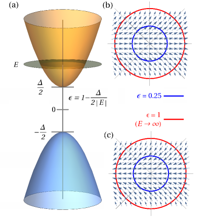
Figure 1: (a) The band structure given by the eigenvalues of (1) is parabolic and isotropic. The energy $E$ is measured from the middle of the bandgap and characterized by the dimensionless parameter $\epsilon$ changing between $0$ (band edge) and $1$ (theoretical limit $|E|\gg\Delta/2$). The in-plane pseudospin texture for conduction (b) and valence (c) bands suggests anisotropic scattering even for isotropic delta-correlated disorder. At $\epsilon\ll 1$, it emulates the pseudospin texture for carriers in phosphorene.

Model. — Having phosphorene Rudenko and Katsnelson (2014) and phosphorene-like materials Gomes and Carvalho (2015) in mind we, however, address a much more general problem. Assume we have a 2D electron gas confined in a 2D conductor whose lattice symmetry determines an effective two-band Hamiltonian that combines Dirac- and Schrödinger-like features given by

$$\hat{H}=\left(\begin{array}[]{cc}\frac{\hbar^{2}k_{y}^{2}}{2m}&\frac{\Delta_{k_{x}}}{2}-i\hbar k_{y}\sqrt{\frac{\Delta_{k_{x}}}{2m}}\\ \frac{\Delta_{k_{x}}}{2}+i\hbar k_{y}\sqrt{\frac{\Delta_{k_{x}}}{2m}}&-\frac{\hbar^{2}k_{y}^{2}}{2m}\end{array}\right),$$ (1)

where $m$ is the effective mass, and $\Delta_{k_{x}}=\Delta+\hbar^{2}k_{x}^{2}/m$ with $\Delta$ being the fundamental bandgap. The spectrum has two branches $E^{\pm}_{k}=\pm E$, see Fig. 1(a), with $E=\frac{\Delta}{2}+\frac{\hbar^{2}k^{2}}{2m}$ and $k^{2}=k_{x}^{2}+k_{y}^{2}$, corresponding to two eigenstates

$$\psi^{+}_{k}=\left(\begin{array}[]{c}\cos\frac{\theta}{2}\\ \sin\frac{\theta}{2}e^{i\gamma}\end{array}\right),\quad\psi^{-}_{k}=\left(\begin{array}[]{c}\sin\frac{\theta}{2}\\ -\cos\frac{\theta}{2}e^{i\gamma}\end{array}\right).$$ (2)

The following angular variables have been defined:

$$\cos\theta=\epsilon\sin^{2}\phi,\quad\cos\gamma=\frac{1-\cos\theta}{\sin\theta},$$ (3)

$$\sin\gamma=\frac{\sin\phi}{\sin\theta}\sqrt{2\epsilon(1-\cos\theta)},\quad\tan\phi=\frac{k_{y}}{k_{x}},$$ (4)

and $\epsilon=1-\frac{\Delta}{2|E|}$, $0\leq\epsilon\leq 1$. To make the hidden anisotropy apparent we cast our Hamiltonian into the form $\hat{H}=\sum_{i}\hat{\sigma}_{i}{\cal H}_{i}$, where $\hat{\sigma}_{i}$ are the Pauli matrices representing the pseudospin, $i=\{x,y,z\}$, and ${\cal H}_{i}$ are the pseudomagnetic field components. The pseudospin eigenstate expectation values then read

$$\langle\hat{\sigma}_{x}\rangle=\pm\left(1-\epsilon\sin^{2}\phi\right),\quad\langle\hat{\sigma}_{z}\rangle=\pm\epsilon\sin^{2}\phi,$$ (5)

$$\langle\hat{\sigma}_{y}\rangle=\pm\sin\phi\sqrt{2\epsilon(1-\epsilon\sin^{2}\phi)},$$ (6)

and the corresponding pseudospin textures are shown Fig. 1(b,c). The direction of a pseudospin vector strongly depends on $\epsilon$ at $\phi\neq 0,\pi$, whereas at $\phi=0,\pi$ the pseudospin keeps its orientation along the $x$-axis no matter how large $\epsilon$ is. Hence, the pseudospin texture forms a preferred direction along which the texture remains collinear and has no influence on scattering. This direction corresponds to the $x$-axis in our case, see also Appendix for comparison with the pseudospin texture on a phosphorene-like lattice. If electrons are moving in any other direction, then the pseudospin texture reduces electron backscattering that facilitates the transport and makes conductivity anisotropic, see Fig. 2.

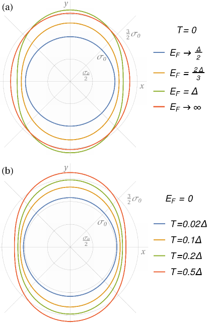
Figure 2: Conductivity $\sigma$ in units of the conventional Drude conductivity $\sigma_{0}=e^{2}\tau_{0}n/m$ as a function of the current direction in the metallic (a) and semiconducting (b) regimes. The Fermi energy is counted from the middle of the bandgap, i.e. it intersects the bottom of the conduction band at $E_{F}=\Delta/2$. The limit $E_{F}\to\infty$ is nonphysical and shown for the sake of completeness.

Boltzmann equation.— We write the Boltzmann equation for electrons assuming that the electron steady-state distribution function, $f_{k}$, is independent of the spatial coordinates and can be written as a sum of equilibrium and non-equilibrium terms, $f_{E\phi}=f^{0}_{E}+f^{x,y}_{E\phi}$, where $f^{x,y}_{E\phi}\ll f^{0}_{E}$. The latter inequality is justified for weak electric field ${\cal E}_{x,y}$ (linear response regime). The Fermi-Dirac distribution $f^{0}_{E}$ is characterized by the Fermi energy $E_{F}$ and temperature $T$ (in energy units). The Boltzmann equation has two components written as

$$e{\cal E}_{x,y}\left\{\begin{array}[]{c}\cos\phi\\ \sin\phi\end{array}\right\}\sqrt{\frac{2E}{m}\epsilon}\frac{\partial f^{0}_{E}}{\partial E}$$ (9)

$$=\int\limits_{0}^{2\pi}d\phi^{\prime}\int\limits_{\Delta/2}^{\infty}\frac{dE^{\prime}m}{(2\pi\hbar)^{2}}w_{EE^{\prime}\phi\phi^{\prime}}\left(f^{x,y}_{E^{\prime}\phi^{\prime}}-f^{x,y}_{E\phi}\right),$$

where $w_{EE^{\prime}\phi\phi^{\prime}}$ is the golden-rule transition probability given by $w_{EE^{\prime}\phi\phi^{\prime}}=\frac{2\pi}{\hbar}n_{i}|U_{EE^{\prime}\phi\phi^{\prime}}|^{2}\delta\left(E-E^{\prime}\right)$. Here, $n_{i}$ is the impurity concentration, and $U_{EE^{\prime}\phi\phi^{\prime}}$ is the scattering potential matrix element. The simplest case is that of a delta-shaped scattering potential with constant Fourier transform $u_{0}$ (see Appendix). Equation (9) can be solved using the Ansatz depending on the electric field direction

$$f^{x,y}_{E\phi}=e{\cal E}_{x,y}\tau_{xx,yy}\left\{\begin{array}[]{c}\cos\phi\\ \sin\phi\end{array}\right\}\sqrt{\frac{2E}{m}\epsilon}\left(-\frac{\partial f^{0}_{E}}{\partial E}\right),$$ (10)

where the momentum relaxation times are given by

$$\tau_{xx}(\phi)= \frac{\tau_{0}}{1-\epsilon\left(\frac{1}{4}+\frac{1-\epsilon}{2}\sin^{2}\phi\right)},$$ (11a)

$$\tau_{yy}(\phi)= \tau_{0}\frac{1+a_{\epsilon}\sqrt{1-\epsilon\sin^{2}\phi}}{1-\epsilon\left(\frac{1}{4}+\frac{1-\epsilon}{2}\sin^{2}\phi\right)},$$ (11b)

and $\tau_{0}^{-1}=n_{i}mu_{0}^{2}/\hbar^{3}$. The relaxation times depend on the electric field direction despite isotropic Fermi surface and disorder. The parameter that makes $\tau_{xx}$ and $\tau_{yy}$ qualitatively different is $a_{\epsilon}$, which we refer to as the ”anomaly parameter”. Its derivation can be found in Appendix. The anomaly parameter is a non-monotonic function of $\epsilon$ but in the low-energy limit it allows for linear approximation $a_{\epsilon}=\epsilon/2$, $\epsilon\ll 1$. Note that our solution (10) holds for arbitrary $a_{\epsilon}$. The momentum relaxation time equals the Bloch lifetime (obtained from Fermi’s golden rule) along $x$, along which the motion is Schrödinger-like, but they are different along all other directions.

Electrical conductivity. — We calculate the electrical current density as

$$j_{x,y}=2e\int\limits_{0}^{2\pi}d\phi\int\limits_{\Delta/2}^{\infty}\frac{dEm}{(2\pi\hbar)^{2}}f^{x,y}_{E\phi}\left\{\begin{array}[]{c}\cos\phi\\ \sin\phi\end{array}\right\}\sqrt{\frac{2E}{m}\epsilon},$$ (12)

where the factor $2$ is due to the spin degeneracy, and $f^{x,y}_{E\phi}$ is given by (10). The conductivity tensor has two components $\sigma_{xx}$ and $\sigma_{yy}$ given by

$$\sigma_{xx}= \frac{e^{2}\tau_{0}}{\pi\hbar^{2}}\int\limits_{\Delta/2}^{\infty}dE\left(E-\frac{\Delta}{2}\right)\left(-\frac{\partial f^{0}_{E}}{\partial E}\right)I_{xx}(E),$$ (13a)

$$\sigma_{yy}= \frac{e^{2}\tau_{0}}{\pi\hbar^{2}}\int\limits_{\Delta/2}^{\infty}dE\left(E-\frac{\Delta}{2}\right)\left(-\frac{\partial f^{0}_{E}}{\partial E}\right)$$ (13b)

$$\times\left[I_{yy}(E)+a_{\epsilon}I_{yy}^{a}(E)\right].$$

Here, $\phi$ was integrated out, and resulting expressions $I_{xx}(E)$, $I_{yy}(E)$, and $I_{yy}^{a}(E)$ are given in Appendix.

We consider two limiting transport regimes: metallic ($E_{F}\geq\Delta/2$, $T\to 0$) and semiconducting ($E_{F}=0$, i.e. the semiconductor is intrinsic). In both cases, the conductivity is anisotropic, and the anisotropy increases with electron energy that can be controlled by either Fermi energy or temperature, depending on the transport regime. The conductivity scaled by $\sigma_{0}=e^{2}n\tau_{0}/m$ is plotted in Fig. 2. Here, $\sigma_{0}$ is the conventional Drude conductivity for Schrödinger carriers, and $n$ is the electron concentration. In the metallic regime Eqs. (13a–13b) can be simplified using the substitution $\left(-\partial f^{0}_{E}/\partial E\right)\to\delta\left(E-E_{F}\right)$, so that $\sigma_{xx}=\sigma_{0}I_{xx}(E_{F})$, and $\sigma_{yy}=\sigma_{0}\left(I_{yy}+a_{\epsilon}I_{yy}^{a}\right)_{E=E_{F}}$. Further simplifications can be performed assuming low doping and using the Taylor-expansion in terms of $1-\Delta/(2E_{F})$ (that is $\epsilon$ taken at $E=E_{F}$). The anisotropy can be then characterized by the ratio

$$\frac{\sigma_{xx}}{\sigma_{yy}}\to\frac{1+3\Delta/(2E_{F})}{4},\quad 1-\frac{\Delta}{2E_{F}}\ll 1.$$ (14)

At $E_{F}=\Delta/2$ the anisotropy disappears but the conductivity vanishes itself in this limit. Hence, the conductivity is anisotropic as long as it is non-zero. The anisotropy is therefore an intrinsic property of our model.

Discussion. — The pseudospin texture depicted in Fig. 1 determines the conductivity anisotropy shown in Fig. 2. Thanks to the texture, disorder affects electrons moving in different directions in a different way. The scattering probability is reduced when the pseudospin has to change its orientation upon scattering. Obviously, the electrons moving along $x$-direction experience no probability reduction for backscattering, as the pseudospin orientation remains the same no matter how large the momentum is. This maximizes resistance and reduces the conductivity $\sigma_{xx}$ to a minimum. In contrast, the carriers moving in any direction other than along $x$-axis have to change the pseudospin orientation upon backscattering. In particular, the pseudospin texture becomes strongly non-collinear for carriers moving along $y$-axis so that the back scattering probability is reduced resulting in an inequality $\sigma_{yy}>\sigma_{xx}$. Certainly, the conductivity is determined not only by the backscattering probability, as the full integral over all possible scattering angles contributes to the electrical resistance. Hence, both $\sigma_{xx}$ and $\sigma_{yy}$ increase with energy as compared with the Drude value $\sigma_{0}$ because the overall non-collinearity of the pseudospin texture becomes stronger. The energy of carriers contributing to the conductance is determined by either the Fermi energy (in the metallic regime) or by temperature (in the semiconducting regime). Thus, the anisotropy can be controlled externally by means of doping and/or heating, as demonstrated in Fig. 2.

The pseudospin eigenstate expectation values (5,6) taken at $\epsilon\ll 1$ emulate the pseudospin texture for carriers in phosphorene Ezawa (2015), see Appendix for references. In this limit, $\langle\hat{\sigma}_{x}\rangle\simeq\pm 1$, $\langle\hat{\sigma}_{z}\rangle\simeq 0$, and $\langle\hat{\sigma}_{y}\rangle\simeq\pm\sin\phi\sqrt{2\epsilon}$, i.e. the in-plane pseudospin collinearity is perfect along the $x$-axis but diminished for other directions, and the out-of-plane component vanishes as long as the higher-order terms in $\epsilon$ are neglected. Similar to phosphorene, our Hamiltonian $\hat{H}$ is time-reversal invariant. Moreover, the eigenstates (3,4) do not produce any Berry curvature or Berry phase. This peculiar property of our Hamiltonian can be understood in terms of the pseudospin field components ${\cal H}_{i}$ defined below Eqs. (3,4). The pseudomagnetic field following the pseudospin direction in Fig. 1(b,c) on a closed trajectory in momentum space does not subtend a solid angle and, hence, results in zero Berry phase. The vanishing Berry curvature is explicitly calculated in Appendix. Note the special relation between ${\cal H}_{i}$ given by $\sqrt{2{\cal H}_{x}{\cal H}_{z}}={\cal H}_{y}$, that makes it possible to exclude ${\cal H}_{z}$ from the Hamiltonian and write all the resulting formulas in terms of ${\cal H}_{y}$ and ${\cal H}_{x}$ only. This also determines a special “equi-pseudospin” curves in momentum space along which the pseudospin does not change. Obviously, any additional term ${\cal H}^{\prime}_{z}\hat{\sigma}_{z}$ would drastically change the geometry and result in non-zero Berry curvature.

The velocity operators derived from (1), given by

$$\hat{v}_{x}= \cos\phi\sqrt{\frac{2E}{m}\epsilon}\,\left(\hat{\sigma}_{x}+\frac{1}{2}\tan\gamma\,\hat{\sigma}_{y}\right),$$ (15a)

$$\hat{v}_{y}= \sin\phi\sqrt{\frac{2E}{m}\epsilon}\,\left(\hat{\sigma}_{z}+\cot\gamma\,\hat{\sigma}_{y}\right),$$ (15b)

resemble the velocity behavior for carriers in phosphorene. At $k\to 0$ (i.e. $\epsilon\to 0$) we find $\tan\gamma\to 0$ and $\hat{v}_{x}\to 0$ (Schrödinger-like behavior) but $\cot\gamma\to\infty$ and $\hat{v}_{y}\to\hat{\sigma}_{y}\sqrt{\frac{\Delta}{2m}}$ (Dirac-like behavior). This also explains why the conductivity is always highest along the $y$-axis: The carriers behave like Dirac particles along this direction, which implies a strong reduction in backscattering. The corresponding group velocities, i.e. the diagonal elements of Eqs. (15a) and (15b) written in the basis of the Hamiltonian eigenstates, are the same as for a conventional electron gas and given by $v_{x}^{\pm}=\pm|v|\cos\phi$, $v_{y}^{\pm}=\pm|v|\sin\phi$ with $|v|=\sqrt{\frac{2E}{m}\epsilon}$. Despite the complexity of the internal structure of our Hamiltonian resembling phosphorene, the spectrum remains isotropic and parabolic. This makes it possible to reveal the hidden conductivity anisotropy at least theoretically. To reveal the effect experimentally in true phosphorene, the band structure anisotropy should be reduced by applying strain Rodin et al. (2014); Wang et al. (2015) or chemical doping Kim et al. (2015); Guo et al. (2016), see also Appendix.

Anisotropic eigenfunctions (3,4) are not something new for Hamiltonians describing 2D electrons with spin-orbit coupling of Rashba Bychkov and Rashba (1984) and Dresselhaus Dresselhaus (1955) types. However, the spin-orbit splitting even being strongly anisotropic by itself does not lead to anisotropic conductivity Trushin and Schliemann (2007). To make the conductivity anisotropic in such heterostructures one has to break time-reversal invariance by adding, e.g. magnetized impurities Trushin et al. (2009). Our Hamiltonian, in contrast, does not break time-reversal and even does not depend on true spin orientation but still leads to a strongly anisotropic conductivity. Furthermore, whereas crystal Hamiltonians are determined from atomic orbitals using symmetry considerations, they may have special properties when the coupling constants have certain values, as is exemplified by the spin helix state in semiconductors with equal Rashba and Dresselhaus interactions. We have studied the special case of a generic Hamiltonian with parameters tuned to achieve an isotropic energy dispersion, which we regard as a dynamical symmetry.

We note that Hamiltonian (1) must be considered within the quasiclassical approximation, where $k_{x,y}$ are just numbers. Otherwise, we have to deal with the pseudo-differential operators that might be a challenging task in the context of scattering. Moreover, we must assume $\sqrt{k_{x}^{2}}=|k_{x}|$ in the theoretical limit $k\to\infty$ ($\epsilon\to 1$) to keep topology the same for any energy and avoid breaking time-reversal invariance in our Hamiltonian. After all, we have to keep the conductivity continuous at $E_{F}\to\infty$. This limit is anyway unrealistic and unphysical leading to a model effect seen in Fig. 2(a). The conductivity and its anisotropy starts to decrease again with $E_{F}$ if the latter is too high. This makes the conductivity non-monotonic as a function of $E_{F}$, see Appendix. In the limit of $\Delta/(2E_{F})\to 0$ (infinite doping or zero bandgap) $a_{\epsilon}=16/(15\pi)$, $I_{xx}=I_{yy}=4/3$, and the anisotropy is $\sigma_{xx}/\sigma_{yy}\to 1/(1+\frac{64}{45\pi^{2}})\sim 0.87$, see Appendix. Formally speaking, the out-of-plane pseudospin components become important at such energies and reduce the non-collinearity of the pseudospin texture. This regime is not related to phosphorene.

Conclusion.— The common belief is that the conductivity anisotropy occurs thanks to either anisotropic Fermi surface or non-scalar disorder (or both). We have found an interesting example in which anisotropy can be induced solely by the internal structure of the effective Hamiltonian comprising Schrödinger and Dirac features. This internal structure does not influence the bands, which always remain parabolic and isotropic, but creates a peculiar pseudospin texture. The texture provides the wave functions with an additional phase depending on the direction of motion. One might think that it is the Berry’s phase that is responsible for this effect but the phase is in fact zero. The origin of conductivity anisotropy is therefore hidden in the Hamiltonian much deeper than just the Berry curvature, and becomes apparent by altering between Dirac and Schrödinger dynamics due to scattering on disorder. This is the reason why this effect is dubbed “hidden anisotropy”. This hidden anisotropy can easily be tuned by changing either the Fermi level or the temperature providing a “hidden knob” for electron transport control.

Acknowledgements. M.T. conceived the project, devised the model, and wrote the draft. A.H.C.N. provided connection to phosphorene. G.V. and D.C. made connection to the vanishing Berry’s phase. M.T. and A.H.C.N. acknowledge funding support from the Singapore National Research Foundation (NRF). In particular, M.T. has been supported by the Director’s Senior Research Fellowship from the CA2DM at NUS (NRF Medium Sized Centre Programme R-723-000-001-281) and by the Gordon Godfrey Bequest while at UNSW. DC is supported by the Australian Research Council Centre of Excellence in Future Low-Energy Electronics Technologies (project number CE170100039) funded by the Australian Government.

Appendix A Construction of a general model with isotropic dispersion and anisotropic conductivity

We look for a model Hamiltonian of the form

$$\hat{H}=h_{x}\hat{\sigma}_{x}+h_{y}\hat{\sigma}_{y}+h_{z}\hat{\sigma}_{z}\,,$$ (16)

where $h_{x}$, $h_{y}$, $h_{z}$ are functions of $k_{x}$ and $k_{y}$, and $\hat{\sigma}_{x,y,z}$ are the Pauli matrices. The dispersion is

$$E_{\pm}=\pm\sqrt{h_{x}^{2}+h_{y}^{2}+h_{z}^{2}}\,.$$ (17)

We want the dispersion to be isotropic, i.e., a function of $k^{2}=k_{x}^{2}+k_{y}^{2}$. Furthermore, we want the Hamiltonian to have a special direction in $k$-space along which the pseudospin orientation (the expectation value of the vector operator $\hat{\sigma}$ in the eigenstate basis of $\hat{H}$) remains constant. (The Berry curvature for such a model will vanish.) This is necessary to make the conductivity anisotropic.

A general way to achieve both requirements is to choose any of the three components of the pseudomagnetic field $\mathbf{h}$, say $h_{y}$, to be the geometric average of the other two:

$$h_{y}=\sqrt{2h_{x}h_{z}}\,.$$ (18)

With this choice the dispersion takes the form

$$E_{\pm}=\pm|h_{x}+h_{z}|\,.$$ (19)

Furthermore, the Hamiltonian takes the form

$$\hat{H}=\sqrt{2h_{x}h_{y}}\left(\hat{\sigma}_{y}+\sqrt{\frac{h_{x}}{2h_{z}}}\hat{\sigma}_{x}+\sqrt{\frac{h_{z}}{2h_{x}}}\hat{\sigma}_{z}\right)\,,$$ (20)

from which it is evident that the orientation of the pseudomagnetic field depends only on the ratio $\frac{h_{z}}{h_{x}}$ and remains constant on the curves along which $h_{z}=\beta h_{x}$, where $\beta=\mathrm{const}$.

Restricting ourselves to polynomials of second order in $k_{x}$ and $k_{y}$ the simplest choice for $h_{x}$ and $h_{z}$ that guarantees an isotropic dispersion is

$$h_{x}=ak_{x}^{2}+bk_{y}^{2}+\Delta_{x}\,,\quad h_{z}=ak_{y}^{2}+bk_{x}^{2}+\Delta_{z}\,,$$ (21)

where $a$, $b$, $\Delta_{x}$, and $\Delta_{y}$ are constants. This gives the isotropic dispersion

$$E_{\pm}=\pm|(a+b)k^{2}+(\Delta_{x}+\Delta_{z})|\,.$$ (22)

Notice that, while the dispersion depends only on the combinations $a+b$ and $\Delta_{x}+\Delta_{z}$, the curves of constant pseudomagnetic field direction depend separately on each of these parameters.

The Hamiltonian discussed in our paper corresponds to the choice

$$a=\frac{\hbar^{2}}{2m},\quad\Delta_{x}=\frac{\Delta}{2},\quad b=0,\quad\Delta_{z}=0\,.$$ (23)

Thus we have

$$h_{x}=\frac{\hbar^{2}k_{x}^{2}}{2m}+\frac{\Delta}{2},\quad h_{y}=\frac{\hbar k_{y}}{\sqrt{m}}\sqrt{\frac{\hbar^{2}k_{x}^{2}}{2m}+\frac{\Delta}{2}},\quad h_{z}=\frac{\hbar^{2}k_{y}^{2}}{2m}.$$ (24)

In the low-energy limit

$$\frac{\hbar^{2}}{2m}\left(k_{x}^{2}+k_{y}^{2}\right)\ll\frac{\Delta}{2}$$ (25)

the pseudomagnetic field preferably polarizes pseudospin along $x$-direction, and the resulting pseudospin texture becomes similar to the one of phosphorene, see the next section.

Appendix B Pseudospin texture in true phosphorene

The low-$k$ expansion of the tight-binding Hamiltonian near $\Gamma$-point in the first Brillouin zone for carriers in phosphorene results in Pereira and Katsnelson (2015)

$$\hat{H}_{0}=\left(\begin{array}[]{lr}u_{0}+\eta_{x}k_{x}^{2}+\eta_{y}k_{y}^{2}&\delta+\gamma_{x}k_{x}^{2}+\gamma_{y}k_{y}^{2}+i\chi k_{y}\\ \delta+\gamma_{x}k_{x}^{2}+\gamma_{y}k_{y}^{2}-i\chi k_{y}&u_{0}+\eta_{x}k_{x}^{2}+\eta_{y}k_{y}^{2}\end{array}\right),$$ (26)

where $u_{0}=-0.42\,\mathrm{eV}$, $\eta_{x}=0.58\,\mathrm{eV}\,\mathring{\mathrm{A}}^{2}$, $\eta_{y}=1.01\,\mathrm{eV}\,\mathring{\mathrm{A}}^{2}$, $\delta=0.76\,\mathrm{eV}$, $\chi=5.25\,\mathrm{eV}\,\mathring{\mathrm{A}}$, $\gamma_{x}=3.93\,\mathrm{eV}\,\mathring{\mathrm{A}}^{2}$, $\gamma_{y}=3.83\,\mathrm{eV}\,\mathring{\mathrm{A}}^{2}$. The single-particle spectrum is given by $E_{\pm}=u_{0}+\eta_{x}k_{x}^{2}+\eta_{y}k_{y}^{2}\pm\sqrt{(\delta+\gamma_{x}k_{x}^{2}+\gamma_{y}k_{y}^{2})^{2}+\chi^{2}k_{y}^{2}}$, where $\pm$ stands for conduction (valence) band. The band gap is then given by $\Delta=2\delta\simeq 1.5$ eV. The eigenstates read $\psi_{\pm}=\frac{1}{\sqrt{2}}(1,\pm e^{i\zeta})^{T}$, where

$$\tan\zeta=\frac{\chi k_{y}}{\delta+\gamma_{x}k_{x}^{2}+\gamma_{y}k_{y}^{2}}.$$ (27)

The carriers in phosphorene obviously obey an anisotropic dispersion and can be described in terms of the corresponding effective masses Pereira and Katsnelson (2015) with the ratios given by

$$\frac{m_{y}^{e}}{m_{x}^{e}}=\frac{\eta_{x}+\gamma_{x}}{\eta_{y}+\gamma_{y}+\chi^{2}/\Delta}\simeq 0.2;\qquad\frac{m_{y}^{h}}{m_{x}^{h}}=\frac{\gamma_{x}-\eta_{x}}{\gamma_{y}+\chi^{2}/\Delta-\eta_{y}}\simeq 0.16$$ (28)

for electrons and holes respectively.

However, the dispersion alone does not match the nature of carriers which is different in different directions. Indeed, the velocity operators $v_{x,y}$ in the lowest order in $k_{x,y}$ have the form

$$\hat{v}_{x}=\left(\begin{array}[]{lr}\eta_{x}&\gamma_{x}\\ \gamma_{x}&\eta_{x}\end{array}\right)\frac{2k_{x}}{\hbar},\qquad\hat{v}_{y}=\left(\begin{array}[]{lr}0&i\chi\\ -i\chi&0\end{array}\right)\frac{1}{\hbar}.$$ (29)

Near the band edge, $v_{x}$ vanishes, whereas $v_{y}$ remains constant. Hence, it should be a qualitative difference in carrier motion along $x$ and $y$ directions. It is especially apparent if we plot the pseudospin texture in momentum space by calculating the pseudospin eigenstate values as $\langle\psi_{\pm}\lvert\hat{\sigma}_{x}\rvert\psi_{\pm}\rangle=\pm\cos\zeta$, $\langle\psi_{\pm}\lvert\hat{\sigma}_{y}\rvert\psi_{\pm}\rangle=\pm\sin\zeta$, where $\hat{\sigma}_{x,y}$ are the Pauli matrices, and $\psi_{\pm}$ are the eigenstates of $H_{0}$. The pseudospin texture is plotted in figure 3.

Unfortunately, the conductivity anisotropy associated with the pseudospin texture is masked by the band anisotropy in phosphorene. Indeed, the ratio $\sigma_{xx}/\sigma_{yy}=m_{y}/m_{x}$ within the Drude model suggests the anisotropy 1:5, whereas the pseudospin texture can provide the conductivity anisotropy up to about 3:4. It is however possible to tune the hoping parameters in the phosphorene-like lattice model to make the conduction and valence bands isotropic but retain the original pseudospin texture. We should first neglect $\eta_{x,y}$, as $\eta_{x,y}\ll\gamma_{x,y}$ anyway. Then, we should satisfy the following equation

$$\Delta(\gamma_{x}-\gamma_{y})=\chi^{2}$$ (30)

to make $m_{y}^{e,h}=m_{x}^{e,h}$. Note that $\gamma_{y}$ depends on the hopping parameters $t_{1}$, $t_{2}$, $t_{3}$, and $t_{5}$, whereas $\gamma_{x}$ depends on $t_{1}$ and $t_{3}$ only, see Refs. Pereira and Katsnelson (2015); Rudenko and Katsnelson (2014). Hence, changing $t_{2}$ or $t_{5}$ we can tune the difference $\gamma_{x}-\gamma_{y}$ to satisfy equation (30) and in that way create a lattice model with isotropic effective masses for electrons and holes. Alternatively, we can utilize substitutional doping Guo et al. (2016) to control the conventional anisotropy.

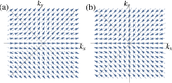
Figure 3: Pseudospin texture in true phosphorene: (a) conduction band, (b) valence band. The region in $k$-space shown has dimensions $1\,\mathring{\mathrm{A}}^{-1}\times 1\,\mathring{\mathrm{A}}^{-1}$. Our Hamiltonian (1) emulates this texture near the band edges ($\epsilon\ll 1$).

Appendix C Solution of the Boltzmann equation

Here we show that our Ansatz (8) solves equation (7). To begin with, the matrix element for a delta-shaped scattering potential is given by:

$$|U_{EE^{\prime}\phi\phi^{\prime}}|^{2}=\frac{u_{0}^{2}}{2}\left[1+\cos\theta\cos\theta^{\prime}+\sin\theta\sin\theta^{\prime}\cos\left(\gamma-\gamma^{\prime}\right)\right].$$ (31)

We first transform equation (31) using equations (3,4) as

$$|U_{EE^{\prime}\phi\phi^{\prime}}|^{2}=u_{0}^{2}\left[1-\frac{1}{2}\left(\cos\theta+\cos\theta^{\prime}\right)+\cos\theta\cos\theta^{\prime}\right.$$

$$\left.+\epsilon\sin\phi\sin\phi^{\prime}\sqrt{1-\cos\theta}\sqrt{1-\cos\theta^{\prime}}\right]$$ (32)

$$=u_{0}^{2}\left[1-\frac{\epsilon}{2}\left(\sin^{2}\phi+\sin^{2}\phi^{\prime}\right)+\epsilon^{2}\sin^{2}\phi\sin^{2}\phi^{\prime}\right.$$

$$\left.+\epsilon\sin\phi\sin\phi^{\prime}\sqrt{1-\epsilon\sin^{2}\phi^{\prime}}\sqrt{1-\epsilon\sin^{2}\phi}\right].$$ (33)

Equation (33) suggests that $|U_{EE^{\prime}0\pi}|^{2}=u_{0}^{2}$ for $\phi=0$ and $\phi^{\prime}=\pi$, i.e. backscattering is very efficient along $x$-axis. In contrast, $|U_{EE^{\prime}\frac{\pi}{2}\frac{3\pi}{2}}|^{2}=u_{0}^{2}(1-2\epsilon+2\epsilon^{2})$ for $\phi=\pi/2$ and $\phi^{\prime}=3\pi/2$, i.e. the backscattering probability is strongly reduced along $y$-axis, and the strongest reduction occurs at $\epsilon=1/2$. Fig. 4 illustrates the angular dependence of $|U_{EE^{\prime}\phi\phi^{\prime}}|^{2}$ for $\phi^{\prime}=0$, $\phi^{\prime}=\pi/4$ and $\phi^{\prime}=\pi/2$. The dependence is especially interesting at $\phi^{\prime}=\pi/4$ in the limit $\epsilon=1$, when it transforms into a strongly asymmetric cardioid-shaped pattern.

If electric field is along $x$-axis, then the Boltzmann equation reads

$$e{\cal E}_{x}\cos\phi\sqrt{\frac{2E}{m}\epsilon}\frac{\partial f^{0}_{E}}{\partial E}=\int\limits_{0}^{2\pi}d\phi^{\prime}\int\limits_{\Delta/2}^{\infty}\frac{dE^{\prime}m}{(2\pi\hbar)^{2}}w_{EE^{\prime}\phi\phi^{\prime}}\left(f^{x}_{E^{\prime}\phi^{\prime}}-f^{x}_{E\phi}\right).$$ (34)

Making use of the delta-function in the scattering probability $w_{EE^{\prime}\phi\phi^{\prime}}$ we have

$$-\cos\phi=\int\limits_{0}^{2\pi}\frac{d\phi^{\prime}m}{(2\pi\hbar)^{2}}w_{EE^{\prime}\phi\phi^{\prime}}\left[\cos\phi^{\prime}\tau_{xx}(\phi^{\prime})-\cos\phi\tau_{xx}(\phi)\right],$$ (35)

The first term on the r.h.s. vanishes after integration over $\phi^{\prime}$. The second term contains the following integral

$$\int\limits_{0}^{2\pi}\frac{d\phi^{\prime}}{2\pi}\left[1-\frac{\epsilon}{2}\left(\sin^{2}\phi+\sin^{2}\phi^{\prime}\right)+\epsilon^{2}\sin^{2}\phi\sin^{2}\phi^{\prime}\right.$$

$$\left.+\epsilon\sin\phi\sin\phi^{\prime}\sqrt{1-\epsilon\sin^{2}\phi^{\prime}}\sqrt{1-\epsilon\sin^{2}\phi}\right]$$

$$=1-\frac{\epsilon}{4}-\frac{1-\epsilon}{2}\epsilon\sin^{2}\phi.$$ (36)

Introducing $\tau_{0}^{-1}=n_{i}mu_{0}^{2}/\hbar^{3}$ we find $\tau_{xx}$ is given by equation (9a), i.e. our solution is correct.

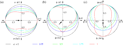
Figure 4: Scattering matrix element squared (33) in units of $u_{0}^{2}$ as a function of scattering angle $\phi$ for different incident angles shown by thick arrows: (a) $\phi^{\prime}=0$, (b) $\phi^{\prime}=\pi/4$, and (c) $\phi^{\prime}=\pi/2$.

If electric field is along $y$-axis, then the Boltzmann equation reads

$$e{\cal E}_{y}\sin\phi\sqrt{\frac{2E}{m}\epsilon}\frac{\partial f^{0}_{E}}{\partial E}=\int\limits_{0}^{2\pi}d\phi^{\prime}\int\limits_{\Delta/2}^{\infty}\frac{dE^{\prime}m}{(2\pi\hbar)^{2}}w_{EE^{\prime}\phi\phi^{\prime}}\left(f^{y}_{E^{\prime}\phi^{\prime}}-f^{y}_{E\phi}\right),$$ (37)

that can again be simplified utilizing the delta-function in the scattering probability as

$$-\sin\phi=\int\limits_{0}^{2\pi}\frac{d\phi^{\prime}m}{(2\pi\hbar)^{2}}w_{EE^{\prime}\phi\phi^{\prime}}\left[\sin\phi^{\prime}\tau_{yy}(\phi^{\prime})-\sin\phi\tau_{yy}(\phi)\right],$$ (38)

Using equations (9b) and (36) the r.h.s. of equation (38) can be rewritten as

$$-\sin\phi=\sin\phi\left[\sqrt{1-\epsilon\sin^{2}\phi}\left(I_{1}+a_{\epsilon}I_{2}\right)-\left(1+a_{\epsilon}\sqrt{1-\epsilon\sin^{2}\phi}\right)\right],$$ (39)

where

$$I_{1}=\epsilon\int\limits_{0}^{2\pi}\frac{d\phi^{\prime}}{2\pi}\frac{\sin^{2}\phi^{\prime}\sqrt{1-\epsilon\sin^{2}\phi^{\prime}}}{1-\epsilon\left(\frac{1}{4}+\frac{1-\epsilon}{2}\sin^{2}\phi^{\prime}\right)},$$ (40)

and

$$I_{2}=\epsilon\int\limits_{0}^{2\pi}\frac{d\phi^{\prime}}{2\pi}\frac{\sin^{2}\phi^{\prime}\left[1-\epsilon\sin^{2}\phi^{\prime}\right]}{1-\epsilon\left(\frac{1}{4}+\frac{1-\epsilon}{2}\sin^{2}\phi^{\prime}\right)}.$$ (41)

Equation (39) is algebraic with respect to $a_{\epsilon}$ and the latter can be determined in terms of $I_{1}$ and $I_{2}$ as

$$a_{\epsilon}=\frac{I_{1}}{1-I_{2}}.$$ (42)

Hence, we have solved the Boltzmann equation using our Ansatz with $a_{\epsilon}$ given by equation (42) and shown in Figure 5.

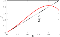
Figure 5: The anomaly parameter $a_{\epsilon}$ (red solid curve) and its low-energy approximation (dashed line).

Appendix D Conductivity integrals

The conductivity is calculated straightforwardly in terms of the following integrals

$$I_{xx} = \int\limits_{0}^{2\pi}\frac{d\phi^{\prime}}{\pi}\frac{\cos^{2}\phi}{1-\epsilon\left(\frac{1}{4}+\frac{1-\epsilon}{2}\sin^{2}\phi^{\prime}\right)}$$ (43)

$$= \frac{8}{4-\epsilon+\sqrt{(\epsilon-4)[4+\epsilon(2\epsilon-3)]}},$$

$$I_{yy} = \int\limits_{0}^{2\pi}\frac{d\phi^{\prime}}{\pi}\frac{\sin^{2}\phi}{1-\epsilon\left(\frac{1}{4}+\frac{1-\epsilon}{2}\sin^{2}\phi^{\prime}\right)}$$ (44)

$$= \frac{8}{4-\epsilon(2\epsilon-3)+\sqrt{(\epsilon-4)[4+\epsilon(2\epsilon-3)]}},$$

and

$$I_{yy}^{a} = \int\limits_{0}^{2\pi}\frac{d\phi^{\prime}}{\pi}\frac{\sin^{2}\phi\sqrt{1-\epsilon\sin^{2}\phi}}{1-\epsilon\left(\frac{1}{4}+\frac{1-\epsilon}{2}\sin^{2}\phi^{\prime}\right)}$$

with an obvious relation

$$I_{1}=\frac{\epsilon}{2}I_{yy}^{a}.$$ (45)

The low-temperature conductivity ratio characterizing the anisotropy is given by

$$\frac{\sigma_{xx}}{\sigma_{yy}}=\left.\frac{I_{xx}}{I_{yy}+a_{\epsilon}I_{yy}^{a}}\right|_{E=E_{F}}$$ (46)

and plotted in figure 6.

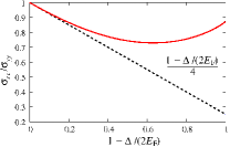
Figure 6: Conductivity ratio $\sigma_{xx}/\sigma_{yy}$ (red solid curve) and its linear approximation (dashed line) in the metallic regime ($E_{F}>\Delta/2$, $T=0$). Note the non-monotonic dependence.

The conductivity can be expressed in units of the Drude conductivity $\sigma_{0}=e^{2}\tau_{0}n/m$, where the electron concentration is given by

$$n=\left\{\begin{array}[]{ll}\frac{m}{\pi\hbar^{2}}\left(E_{F}-\frac{\Delta}{2}\right),&\mathrm{metallic};\\ \frac{m}{\pi\hbar^{2}}\left[T\ln\left(1+e^{\frac{\Delta}{2T}}\right)-\frac{\Delta}{2}\right],&\mathrm{semiconducting}.\end{array}\right.$$ (47)

Appendix E Berry curvature calculation

The Berry curvature vanishes for Hamiltonian (1). Here, we show that it is indeed so by direct calculation. In general, Berry curvature is a vector given by a cross-product of two vectors $\vec{\Omega}=i\langle\nabla_{\mathbf{k}}\psi_{k}\rvert\times\lvert\nabla_{\mathbf{k}}\psi_{k}\rvert\rangle$. In our case, it has only $z$-component given by

$$\Omega=-\frac{1}{2}\sin\theta\left(\partial_{k_{x}}\theta\partial_{k_{y}}\gamma-\partial_{k_{x}}\gamma\partial_{k_{y}}\theta\right),$$ (48)

where

$$\tan\gamma=\sqrt{\frac{2\hbar^{2}}{m\Delta_{k_{x}}}}k_{y},\quad\tan\theta=\frac{\sqrt{\frac{\Delta_{k_{x}}^{2}}{4}+\frac{\hbar^{2}k_{y}^{2}}{2m}\Delta_{k_{x}}}}{\frac{\hbar^{2}k_{y}^{2}}{2m}},\quad\Delta_{k_{x}}=\Delta+\frac{\hbar^{2}k_{x}^{2}}{m}.$$ (49)

Taking derivatives we have

$$\frac{\partial\gamma}{\partial k_{x}}=-\frac{\hbar^{2}k_{x}k_{y}}{m\Delta_{k_{x}}}\frac{\partial\gamma}{\partial k_{y}},\quad\frac{\partial\gamma}{\partial k_{y}}=\frac{\sqrt{\frac{2\hbar^{2}}{m\Delta_{k_{x}}}}}{1+\frac{2\hbar^{2}k_{y}^{2}}{m\Delta_{k_{x}}}},$$ (50)

$$\frac{\partial\theta}{\partial k_{x}}=\frac{E}{\sqrt{\frac{\Delta_{k_{x}}^{2}}{4}+\frac{\hbar^{2}k_{y}^{2}}{2m}\Delta_{k_{x}}}}\frac{1}{1+\frac{\frac{\Delta_{k_{x}}^{2}}{4}+\frac{\hbar^{2}k_{y}^{2}}{2m}\Delta_{k_{x}}}{\left(\frac{\hbar^{2}k_{y}^{2}}{2m}\right)^{2}}}\frac{\frac{\hbar^{2}k_{x}}{m}}{\frac{\hbar^{2}k_{y}^{2}}{2m}},$$ (51)

$$\frac{\partial\theta}{\partial k_{y}}=-\frac{E}{\sqrt{\frac{\Delta_{k_{x}}^{2}}{4}+\frac{\hbar^{2}k_{y}^{2}}{2m}\Delta_{k_{x}}}}\frac{1}{1+\frac{\frac{\Delta_{k_{x}}^{2}}{4}+\frac{\hbar^{2}k_{y}^{2}}{2m}\Delta_{k_{x}}}{\left(\frac{\hbar^{2}k_{y}^{2}}{2m}\right)^{2}}}\frac{\frac{\Delta_{k_{x}}}{2}\frac{\hbar^{2}k_{y}}{m}}{\left(\frac{\hbar^{2}k_{y}^{2}}{2m}\right)^{2}}.$$ (52)

Finally, we sum up all the terms and obtain

$$\Omega=-\frac{1}{2}\sin\theta\frac{E}{\sqrt{\frac{\Delta_{k_{x}}^{2}}{4}+\frac{\hbar^{2}k_{y}^{2}}{2m}\Delta_{k_{x}}}}\frac{1}{1+\frac{\frac{\Delta_{k_{x}}^{2}}{4}+\frac{\hbar^{2}k_{y}^{2}}{2m}\Delta_{k_{x}}}{\left(\frac{\hbar^{2}k_{y}^{2}}{2m}\right)^{2}}}\frac{\sqrt{\frac{2\hbar^{2}}{m\Delta_{k_{x}}}}}{1+\frac{2\hbar^{2}k_{y}^{2}}{m\Delta_{k_{x}}}}\left[\frac{\frac{\hbar^{2}k_{x}}{m}}{\frac{\hbar^{2}k_{y}^{2}}{2m}}-\frac{\hbar^{2}k_{x}k_{y}}{m\Delta_{k_{x}}}\frac{\frac{\Delta_{k_{x}}}{2}\frac{\hbar^{2}k_{y}}{m}}{\left(\frac{\hbar^{2}k_{y}^{2}}{2m}\right)^{2}}\right].$$ (53)

The expression in the square brackets is zero. Hence, $\Omega=0$.

References

Bhimanapati et al. (2015)
G. R. Bhimanapati,
Z. Lin,
V. Meunier,
Y. Jung,
J. Cha,
S. Das,
D. Xiao,
Y. Son,
M. S. Strano,
V. R. Cooper,
et al., ACS Nano
9, 11509 (2015).
Novoselov et al. (2016)
K. Novoselov,
A. Mishchenko,
A. Carvalho, and
A. Castro Neto,
Science 353,
aac9439 (2016).
Castro Neto et al. (2009)
A. H. Castro Neto,
F. Guinea,
N. M. R. Peres,
K. S. Novoselov,
and A. K. Geim,
Reviews of Modern Physics 81,
109 (2009).
DasSarma et al. (2011)
S. DasSarma,
S. Adam,
E. H. Hwang, and
E. Rossi,
Reviews of Modern Physics 83,
407 (2011).
Adam et al. (2007)
S. Adam,
E. Hwang,
V. Galitski, and
S. D. Sarma,
Proceedings of the National Academy of Sciences
104, 18392
(2007).
Trushin et al. (2010)
M. Trushin,
J. Kailasvuori,
J. Schliemann,
and A. H.
MacDonald, Phys. Rev. B
82, 155308
(2010).
Dean et al. (2010)
C. R. Dean,
A. F. Young,
I. Meric,
C. Lee,
L. Wang,
S. Sorgenfrei,
K. Watanabe,
T. Taniguchi,
P. Kim,
K. L. Shepard,
et al., Nature Nanotechnology
5, 722 (2010).
Cao et al. (2018)
Y. Cao,
V. Fatemi,
S. Fang,
K. Watanabe,
T. Taniguchi,
E. Kaxiras, and
P. Jarillo-Herrero,
Nature 556, 43
(2018).
Kane and Mele (2005)
C. L. Kane and
E. J. Mele,
Phys. Rev. Lett. 95,
146802 (2005).
Hasan and Kane (2010)
M. Z. Hasan and
C. L. Kane,
Reviews of Modern Physics 82,
3045 (2010).
Fu and Kane (2008)
L. Fu and
C. L. Kane,
Phys. Rev. Lett. 100,
096407 (2008).
Mak et al. (2014)
K. F. Mak,
K. L. McGill,
J. Park, and
P. L. McEuen,
Science 344,
1489 (2014).
Dai et al. (2017)
X. Dai,
Z. Z. Du, and
H. Z. Lu,
Phys. Rev. Lett. 119,
166601 (2017).
Breunig et al. (2017)
O. Breunig,
Z. Wang,
A. A. Taskin,
J. Lux,
A. Rosch, and
Y. Ando,
Nature Communications 8,
15545 (2017).
Yasuda et al. (2016)
K. Yasuda,
A. Tsukazaki,
R. Yoshimi,
K. S. Takahashi,
M. Kawasaki, and
Y. Tokura,
Phys. Rev. Lett. 117,
127202 (2016).
He et al. (2018)
P. He,
S. Zhang,
D. Zhu,
Y. Liu,
Y. Wang,
J. Yu,
G. Vignale, and
H. Yang,
Nature Physics 14,
495 (2018).
Ando et al. (1982)
T. Ando,
A. B. Fowler,
and F. Stern,
Reviews of Modern Physics 54,
437 (1982).
Sundaram and Niu (1999)
G. Sundaram and
Q. Niu,
Phys. Rev. B 59,
14915 (1999).
McCann and Fal’ko (2006)
E. McCann and
V. I. Fal’ko,
Phys. Rev. Lett. 96,
086805 (2006).
Ribeiro and Peres (2011)
R. M. Ribeiro and
N. M. R. Peres,
Phys. Rev. B 83,
235312 (2011).
Xiao et al. (2012)
D. Xiao,
G.-B. Liu,
W. Feng,
X. Xu, and
W. Yao,
Phys. Rev. Lett. 108,
196802 (2012).
Pereira and Katsnelson (2015)
J. M. Pereira and
M. I. Katsnelson,
Phys. Rev. B 92,
075437 (2015).
Trushin and Schliemann (2011)
M. Trushin and
J. Schliemann,
Phys. Rev. Lett. 107,
156801 (2011).
Liu et al. (2014)
H. Liu,
A. T. Neal,
Z. Zhu,
Z. Luo,
X. Xu,
D. Tom nek,
and P. D. Ye,
ACS Nano 8,
4033 (2014).
Lu et al. (2016)
J. Lu,
J. Yang,
A. Carvalho,
H. Liu,
Y. Lu, and
C. H. Sow,
Accounts of Chemical Research
49, 1806 (2016).
Carvalho et al. (2016)
A. Carvalho,
M. Wang,
X. Zhu,
A. S. Rodin,
H. Su, and
A. H. Castro Neto,
Nature Reviews Materials 1,
16061 (2016).
Rodin et al. (2014)
A. S. Rodin,
A. Carvalho, and
A. H. Castro Neto,
Phys. Rev. Lett. 112,
176801 (2014).
Fukuoka et al. (2015)
S. Fukuoka,
T. Taen, and
T. Osada,
Journal of the Physical Society of Japan
84, 121004
(2015).
Ezawa (2015)
M. Ezawa, in
Journal of Physics: Conference Series
(IOP Publishing, 2015), vol.
603, p. 012006.
Zare et al. (2017)
M. Zare,
B. Z. Rameshti,
F. G. Ghamsari,
and R. Asgari,
Phys. Rev. B 95,
045422 (2017).
Rudenko and Katsnelson (2014)
A. N. Rudenko and
M. I. Katsnelson,
Phys. Rev. B 89,
201408(R) (2014).
Gomes and Carvalho (2015)
L. C. Gomes and
A. Carvalho,
Phys. Rev. B 92,
085406 (2015).
Wang et al. (2015)
L. Wang,
A. Kutana,
X. Zou, and
B. I. Yakobson,
Nanoscale 7,
9746 (2015).
Kim et al. (2015)
J. Kim,
S. S. Baik,
S. H. Ryu,
Y. Sohn,
S. Park,
B.-G. Park,
J. Denlinger,
Y. Yi,
H. J. Choi, and
K. S. Kim,
Science 349,
723 (2015).
Guo et al. (2016)
C. Guo,
C. Xia,
L. Fang,
T. Wang, and
Y. Liu,
Physical Chemistry Chemical Physics
18, 25869 (2016).
Bychkov and Rashba (1984)
Y. A. Bychkov and
E. I. Rashba,
JETP Lett. 39,
78 (1984).
Dresselhaus (1955)
G. Dresselhaus,
Phys. Rev. 100,
580 (1955).
Trushin and Schliemann (2007)
M. Trushin and
J. Schliemann,
Phys. Rev. B 75,
155323 (2007).
Trushin et al. (2009)
M. Trushin,
K. Výborný,
P. Moraczewski,
A. A. Kovalev,
J. Schliemann,
and
T. Jungwirth,
Phys. Rev. B 80,
134405 (2009).