Two- and three-pion finite-volume spectra at maximal isospin from lattice QCD

Abstract

We present the three-pion spectrum with maximal isospin in a finite volume determined from lattice QCD, including excited states in addition to the ground states across various irreducible representations at zero and nonzero total momentum. The required correlation functions, from which the spectrum is extracted, are computed using a newly implemented algorithm which speeds up the computation by more than an order of magnitude. On a subset of the data we extract a nonzero value of the three-pion threshold scattering amplitude using the $1/L$ expansion of the three-particle quantization condition, which consistently describes all states at zero total momentum. The finite-volume spectrum is publicly available to facilitate further explorations within the available three-particle finite-volume approaches.

I Introduction

Lattice QCD calculations of scattering amplitudes have matured significantly over the last decade owing to marked increases in available computational capacity and improved algorithms. A widely used approach for constraining scattering observables from simulations relies on precise measurements of the interacting energy levels of QCD in a finite volume, which encode hadron interactions via the shifts from their noninteracting values Luscher (1986a, b); Lüscher (1991); Luscher and Wolff (1990); Rummukainen and Gottlieb (1995) (see Briceño et al. (2017a) for a survey of extensions of the formalism and numerical results).

So far, practical calculations in lattice QCD have been mostly confined to the two-hadron sector. Though a large abundance of lattice data is currently available for scattering of two hadrons (e.g. $\pi\pi$ scattering in all three isospin channels Beane et al. (2006, 2008a); Feng et al. (2010, 2011); Beane et al. (2012); Lang et al. (2011); Aoki et al. (2011); Pelissier and Alexandru (2013); Dudek et al. (2012, 2013); Sasaki et al. (2014); Fu (2013); Wilson et al. (2015); Helmes et al. (2015); Bali et al. (2016); Bulava et al. (2016); Guo et al. (2016); Fu and Wang (2016); Briceño et al. (2017b); Liu et al. (2017); Alexandrou et al. (2017); Briceno et al. (2018); Andersen et al. (2019); Guo et al. (2018); Culver et al. (2019), see also Kurth et al. (2013); Akahoshi et al. (2019) for results using a potential-based approach), these calculations are formally restricted to energies below thresholds involving three or more hadrons due to the use of a formalism for relating finite-volume spectra to scattering amplitudes that is limited to two-hadron scattering. This limitation has precluded a proper lattice QCD study of systems involving three or more stable hadrons at light pion masses, e.g. the Roper resonance which decays to both two- and three-particle channels, the $\omega(782)$ decaying to three pions, many of the $X$, $Y$ and $Z$ resonances, and three-nucleon interactions relevant for nuclear physics.

Following the demonstration that the finite-volume spectrum is determined by the infinite-volume $S$ matrix, even in the presence of three-particle intermediate states Polejaeva and Rusetsky (2012), significant progress has been made in developing the necessary formalism to interpret the three-particle finite-volume spectrum, both by extending the two-particle derivation to include three-hadron states Hansen and Sharpe (2014, 2015); Briceño et al. (2017c, 2019), as well as through alternative approaches Agadjanov et al. (2016); Hammer et al. (2017a, b); Mai and Döring (2017); Döring et al. (2018) (for a review see Hansen and Sharpe (2019)). Thus, although the three-particle formalism is quite mature—including numerical explorations of the corresponding quantization conditions Briceño et al. (2018); Romero-López et al. (2018); Mai and Doring (2019)—data for three-particle finite-volume QCD spectra is lacking, since previous lattice QCD calculations have been restricted to the extraction of multi-meson ground states at rest Beane et al. (2008b); Detmold et al. (2008a, b). Recently a first calculation of finite-volume spectra including three-particle energies was carried out in the $b_{1}$ system, whose results are however not yet amenable to an interpretation in the present three-particle formalisms Woss et al. (2019). Hence no comprehensive data exists to apply the available finite-volume formalisms.

We fill this gap by providing the two-pion and three-pion spectra with maximum isospin in various irreducible representations (irreps) at zero and nonzero total momentum in the elastic region, i.e. for center-of-mass energies $E_{\mathrm{cm}}/m_{\pi}$ below 4 and 5 for isospin $I=2$ and $I=3$ respectively. Our analysis of a subset of the data indicates sensitivity to the three-pion interaction at the current level of precision. In order to facilitate a more detailed exploration, possibly including the effect of higher partial waves Blanton et al. (2019); Hansen and Sharpe (2014, 2015); Döring et al. (2018), the spectrum data is made public including all correlations.

A technical challenge concerns the growing number of Wick contractions required to compute correlation functions of suitable interpolating operators—from which the spectrum is extracted—as the number of valence quark fields increases. The continued need for improved algorithms to perform these contractions was pointed out recently Detmold et al. (2019) and indeed was a limiting factor in a recent study of meson-baryon scattering in the $\Delta$ channel Andersen et al. (2018). While Refs. Yamazaki et al. (2010); Detmold and Savage (2010); Doi and Endres (2013); Detmold and Orginos (2013); Günther et al. (2013); Nemura (2016) investigated efficient contraction algorithms at the quark level, we employ the stochastic variant Morningstar et al. (2011) of distillation Peardon et al. (2009) to treat quark propagation. In this framework, it is useful to view the correlation function construction in terms of contractions of tensors associated with the involved hadrons. Then, to reduce the operation count required to evaluate all contractions, we use a method which is well-known in quantum chemistry Hartono et al. (2005, 2006, 2009) and has attracted renewed interest in the context of tensor networks Pfeifer et al. (2014). The proposed optimization achieves a speedup by more than an order of magnitude, can be readily used for general physical systems (e.g. three-meson systems at nonmaximal isospin and two-baryon systems), and its implementation is publicly available .

This letter is organized as follows: We first discuss the interpolating operators employed and construction of their correlation functions, followed by a description of the ensemble used in this work. Subsequently the finite-volume spectra and extraction of two- and three-pion scattering parameters from a subset of the data are presented.

II Lattice QCD methods

Interpolating operators: Lattice simulations of QCD in a cubic box break the infinite-volume $SO(3)$ rotational symmetry. The spectrum in finite volume is customarily extracted employing interpolating operators which transform irreducibly under the symmetries of a cubic spatial lattice, i.e. the octahedral group $O_{h}$ for zero total momentum $\textbf{P}=\textbf{0}$ and the corresponding little groups for $\textbf{P}\neq\textbf{0}$ Dudek et al. (2012); Morningstar et al. (2013). Correlation functions of such interpolators access only the sub-block of the finite-volume Hamiltonian corresponding to the same irrep, thus greatly simplifying the determination of the spectrum and the subsequent scattering-amplitude analysis.

We employ the simplest single-pion operator destroying a three-momentum p given by

$$\pi_{\textbf{p}}(t)=\sum_{\textbf{x}}\mathrm{e}^{-i\textbf{p}\cdot\textbf{x}}\bar{d}(\textbf{x},t)\gamma_{5}u(\textbf{x},t).$$ (1)

This operator transforms in the $A_{1u}^{-}$ and $A_{2}^{-}$ irrep for zero and nonzero momentum respectively, where the superscript specifies the $G$-parity.

Two-pion interpolators which transform according to the irrep $\Lambda$ of the little group of total momentum P are obtained by forming appropriate linear combinations of two single-pion interpolators with momenta $\textbf{p}_{1}+\textbf{p}_{2}=\textbf{P}$,

$$\pi\pi^{(\textbf{P},\Lambda)}(t)=c^{(\textbf{P},\Lambda)}_{\textbf{p}_{1},\textbf{p}_{2}}\pi_{\textbf{p}_{1}}(t)\pi_{\textbf{p}_{2}}(t).$$ (2)

The relevant Clebsch-Gordan coefficients $c^{(\textbf{P},\Lambda)}_{\textbf{p}_{1},\textbf{p}_{2}}$ were worked out in Morningstar et al. (2013) (see also Dudek et al. (2012)) and used previously to study $\pi\pi$ scattering Bulava et al. (2016); Andersen et al. (2019).

Three-pion interpolators are obtained by iterating this process, i.e. by first coupling two of the pions into an intermediate irrep, then using the Clebsch-Gordan coefficients again to obtain operators transforming according to one of the total irreps of interest,

$$\pi\pi\pi^{(\textbf{P},\Lambda)}(t)=c^{(\textbf{P},\Lambda)}_{\textbf{p}_{1},\textbf{p}_{2},\textbf{p}_{3}}\pi_{\textbf{p}_{1}}(t)\pi_{\textbf{p}_{2}}(t)\pi_{\textbf{p}_{3}}(t).$$ (3)

Due to the weak interaction in $I=2$ $\pi\pi$ scattering, which is the only relevant subprocess for this work, the more elaborate operator construction discussed in Woss et al. (2019) is not required. The interpolators we use in this work are listed in the supplemental material.

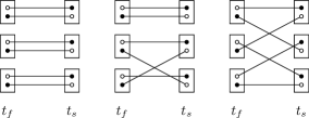
Figure 1: Different topologies of Wick contractions required to evaluate $I=3$ three-pion correlation functions. Circles indicate quark and antiquark fields tied into meson functions shown as boxes, which are subsequently contracted. Two-pion $I=2$ Wick contractions appear as subexpressions.

Correlation function construction: Quark propagation is treated using the stochastic LapH method Morningstar et al. (2011) by first obtaining smeared solutions of the Dirac equation,

$$\varphi^{[r,d]}=\mathcal{S}D^{-1}\varrho^{[r,d]},$$ (4)

for stochastic quark-field sources $\varrho^{[r,d]}$ with noise index $r=1,\dots,N_{\eta}$, dilution Wilcox (1999); Foley et al. (2005) index $d=1,\dots,N_{\mathrm{dil}}$, and where $\mathcal{S}$ is the LapH smearing kernel, formed from the $N_{\mathrm{ev}}$ lowest eigenvectors of the three-dimensional covariant Laplacian. Next, useful intermediate quantities are the pion source and sink functions Morningstar et al. (2011)

$$\mathcal{M}_{\textbf{p}}^{[r_{1},r_{2},d_{1},d_{2}]}(t) =-\sum_{\textbf{x}}\mathrm{e}^{-i\textbf{p}\cdot\textbf{x}}\varrho^{[r_{1},d_{1}]*}_{a\alpha\textbf{x}t}\varrho^{[r_{2},d_{2}]}_{a\alpha\textbf{x}t},$$ (5)

$$\bar{\mathcal{M}}_{\textbf{p}}^{[r_{1},r_{2},d_{1},d_{2}]}(t) =\phantom{-}\sum_{\textbf{x}}\mathrm{e}^{-i\textbf{p}\cdot\textbf{x}}\varphi^{[r_{1},d_{1}]*}_{a\alpha\textbf{x}t}\varphi^{[r_{2},d_{2}]}_{a\alpha\textbf{x}t},$$

with summed color index $a$ and spin index $\alpha$, and two open noise and dilution indices. In terms of these meson functions, the single-pion correlation function on a single gauge configuration is obtained by the average over noise combinations $\{r_{1},r_{2}\}$ Morningstar et al. (2011)

$$C_{\pi_{\textbf{p}}}(t_{f} -t_{s})\propto$$

$$-\sum_{\{r_{1},r_{2}\}}\bar{\mathcal{M}}_{\textbf{p}}^{[r_{1},r_{2},d_{1},d_{2}]}(t_{f})\mathcal{M}_{\textbf{p}}^{[r_{1},r_{2},d_{1},d_{2}]*}(t_{s}),$$ (6)

with proper normalization given by the number of noise combinations used to perform the average.

For a given momentum, pair of source and sink time $t_{s}$ and $t_{f}$, and noise combination, Eq. (6) is a tensor contraction over dilution indices of two rank-2 tensors with index range $N_{\mathrm{dil}}$. Two- and three-pion correlation functions with maximal isospin can be computed using the same building blocks Morningstar et al. (2011) and involve tensor contractions governed by all possible Wick contractions of four and six rank-2 tensors respectively.

The number of Wick contractions grows factorially as more pions are included Beane et al. (2008b), and the different topologies of diagrams for three-pion correlation functions in the sector of maximal isospin are shown in Fig. 1. However, across the relevant diagrams there is a lot of redundancy which can be exploited systematically to reduce the number of arithmetic operations required for their evaluation. In particular, all diagrams required for the computation of $I=2$ two-pion correlation functions appear as subdiagrams of $I=3$ three-pion correlation functions.

The algorithm to automatically perform the operation-count minimization is described in the supplemental material together with a detailed example. For the evaluation of the correlation functions required in this work we achieve a speed-up by roughly a factor of 15.

Table 1: Ensemble and measurement setup used in this work. Measurements are performed on $N_{\mathrm{cfg}}$ configurations with spatial volume $L^{3}$ separated by $4\,\mathrm{MDU}$. Correlation functions are estimated starting from a single source time $t_{s}/a=35$ using $N_{\eta}$ diluted noise sources to estimate quark propagators (see Morningstar et al. (2011) for unexplained notation). Other parameters, e.g. for stout smearing Morningstar and Peardon (2004), are the same as in Andersen et al. (2019).

$am_{\pi}$	$L/a$	$N_{\mathrm{ev}}$	dilution	$N_{\eta}$	$N_{\mathrm{cfg}}$
0.06504(33)	64	448	(TF,SF,LI16)	6	1100

Ensemble details: The results in this work are based on the D200 ensemble generated through the CLS effort Bruno et al. (2015) with $N_{\mathrm{f}}=2+1$ quark flavors at a pion mass $m_{\pi}\approx 200\,\mathrm{MeV}$ and lattice spacing $a\approx 0.064\,\mathrm{fm}$ Bruno et al. (2017). The ensemble and measurement setup is detailed in Table 1. In order to ensure a Hermitian matrix of correlation functions despite the use of open boundary conditions in the temporal direction Lüscher and Schaefer (2011), our interpolating operators are always separated from the temporal boundaries by at least $t_{s}$, where $m_{\pi}t_{s}=2.2$.

Pion-pion scattering in the isovector channel has been investigated on this ensemble previously Andersen et al. (2019), and statistics subsequently improved considerably to provide spectroscopic information for the determination of the hadronic vacuum polarization on the same ensemble Gérardin et al. (2019). The pion functions are re-used from that work, and hence no additional meson functions or solutions of the Dirac equation have to be computed.

III Results

Analysis strategy: The procedure to extract the finite-volume spectrum from a matrix of correlation functions $C_{ij}(t)$ in a given irrep is discussed in detail in Bulava et al. (2016) and we use the analysis suite developed in Andersen et al. (2019).

We solve a generalized eigenvalue problem Michael and Teasdale (1983); Luscher and Wolff (1990); Blossier et al. (2009) for a fixed reference time and diagonalization time $(t_{0}=5a,t_{*}=10a)$, corresponding to roughly $0.32\,\mathrm{fm}$ and $0.64\,\mathrm{fm}$ in physical units Bruno et al. (2017), in order to extract not only the ground state but also excited states in most irreps. Results from different $(t_{0},t_{*})$ are indistinguishable, presumably due to the weak interaction in $I=2$ and $I=3$ pion scattering which results in little mixing of our interpolating operators, in which each hadron has been projected to definite momentum and is hence expected to overlap predominantly with a single state.

For two-pion states the difference $\Delta\!E$ between interacting and noninteracting energies is determined from single-exponential fits at sufficiently large time separations to the ratios

$$R_{i}(t)=\frac{\hat{C}_{ii}(t)}{C_{\pi_{\textbf{p}_{1}}}\!(t)\,C_{\pi_{\textbf{p}_{2}}}\!(t)}\xrightarrow{\mathrm{large}\;t}A\mathrm{e}^{-\Delta\!E_{i}t}$$ (7)

of diagonal elements of the ‘optimized’ correlation matrix $\hat{C}$ Bulava et al. (2016) and two single-pion correlation functions, and similarly for the three-pion states Beane et al. (2008b). Absolute energies are reconstructed from those energy differences using the single-pion dispersion relation. The attainable precision is generally at the few-permille level for the energies measured in units of the single-pion mass.

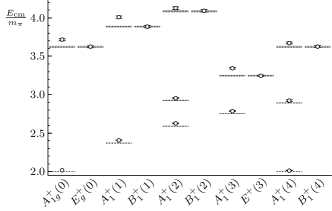
Figure 2: $I=2$ two-pion spectrum in various irreps $\Lambda(\textbf{d}^{2})$ with total momentum $\textbf{P}=\frac{2\pi}{L}\textbf{d}$. Open symbols denote the measured interacting energies which are shifted from their noninteracting values shown as dashed lines.

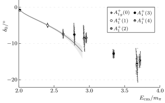
Figure 3: Energy dependence of the $I=2$ $\pi\pi$ s-wave scattering amplitude extracted from the two-pion spectrum. The gray band shows the result of the fit to the five leftmost points using the effective range expansion given in Eq. (8).

Two-pion spectrum and scattering amplitude: The two-pion spectrum with maximal isospin is shown in Fig. 2 together with the noninteracting energies. The respective differences encode the two-pion scattering amplitude for $\ell=0$ shown in Fig. 3 neglecting the effect of higher even partial waves. Its energy dependence for scattering momentum $q^{2}/m_{\pi}^{2}<1$ is described using the effective-range expansion

$$q\cot\delta_{0}=-\frac{1}{a_{0}}+\frac{r_{0}}{2}q^{2},$$ (8)

and the scattering length $a_{0}$ and effective range $r_{0}$ are determined from a fit using the determinant-residual method Morningstar et al. (2017) with $\mu=64$, which yields

$$m_{\pi}a_{0}=0.1019(88),\quad m_{\pi}r_{0}=9.0(2.4),$$ (9)

$$\chi^{2}/\mathrm{dof}=1.33.$$

A comparison of our scattering length with previous lattice QCD determinations Fu (2013); Sasaki et al. (2014); Beane et al. (2006); Feng et al. (2010); Beane et al. (2008a); Dudek et al. (2012); Bulava et al. (2016), together with the experimental value from Ananthanarayan et al. (2001), is shown in the supplemental material .

Three-pion spectrum and $1/L$ expansion: The three-pion spectrum with maximal isospin is shown in Fig. 4, displaying significant energy shifts in all irreps. In particular, interacting energy levels from different irreps that contain some degeneracy of the noninteracting spectra (e.g. $A_{1u}^{-}$ and $E_{u}^{-}$ at zero total momentum) differ substantially, which may suggest sensitivity to different combinations of low-energy scattering parameters.

At leading order in the $1/L$ expansion of the three-particle quantization condition Beane et al. (2007); Detmold and Savage (2008); Hansen and Sharpe (2016); Sharpe (2017); Pang et al. (2019) ,

$$\Delta\!E_{\rm 3}=\frac{12\pi a_{0}}{m_{\pi}L^{3}}\Bigg{\{}1-\Big{(}\frac{a_{0}}{\pi L}\Big{)}\mathcal{I}+\Big{(}\frac{a_{0}}{\pi L}\Big{)}^{2}(\mathcal{I}^{2}+\mathcal{J})+\frac{3\pi a_{0}}{m_{\pi}^{2}L^{3}}\\ +\frac{64\pi^{2}a_{0}^{2}\mathcal{C}_{3}}{m_{\pi}L^{3}}+\frac{6\pi r_{0}a_{0}^{2}}{L^{3}}+\Big{(}\frac{a_{0}}{\pi L}\Big{)}^{3}[c_{L}\log(N_{\rm cut})-\mathcal{I}^{3}+\mathcal{I}\mathcal{J}\\ +15\mathcal{K}+\mathcal{C}_{F}+\mathcal{C}_{4}+\mathcal{C}_{5}]\Bigg{\}}-\frac{\mathcal{M}_{\rm 3,th}}{48m_{\pi}^{3}L^{6}}+O(L^{-7})\,,$$ (10)

the ground-state energy shift $\Delta\!E_{\mathrm{3}}$ is three times larger than the corresponding two-particle shift $\Delta\!E_{2}$ Beane et al. (2008b). The deviation of our numerical result

$$\Delta\!E_{3}/\Delta\!E_{2}=2.78(21),$$ (11)

is due to two-particle effects at higher orders in $1/L$ and the three-pion interaction.

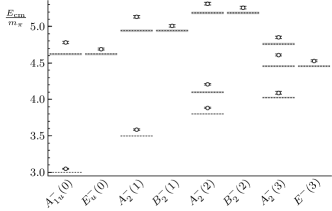
Figure 4: Same as Fig. 2 but for the $I=3$ three-pion spectrum.

Using the two-particle scattering length and effective range determined before, the three-particle threshold scattering amplitude entering at $L^{-6}$ can be isolated and we obtain

$$\frac{m_{\pi}^{2}\mathcal{M}_{\rm 3,th}}{48\,(m_{\pi}L)^{6}}=0.0113(43).$$ (12)

While this quantity depends on how two- and three-particle effects are separated Hansen and Sharpe (2016); Romero-López et al. (2018), within the scheme discussed in those references our result indicates sensitivity to three-particle physics.

Using the nonrelativistic threshold expansion from Ref. Pang et al. (2019) yields a result with similar significance. From that reference, the energy of the excited states at rest are predicted to be

$$A_{1u}^{-}:\quad E_{3}^{\prime}/m_{\pi} =4.76(8),$$ (13)

$$E_{u}^{-}:\quad E_{3}^{\prime}/m_{\pi} =4.72(2),$$

in good agreement with our measured values. Further, the formalism employed in Mai and Doring (2019) with the scattering parameters determined there predicts the first excited state in the at-rest $A_{1u}^{-}$ irrep to be

$$E_{3}^{\prime}/m_{\pi}=4.75$$ (14)

at our pion mass and spatial volume, which is also in agreement with the measured value.

More work along the lines of Döring et al. (2018); Blanton et al. (2019) is required to apply the quantization condition to the energies in all irreps presented here. In order to facilitate further investigations in that direction, the two-pion and three-pion spectra are made publicly available including all correlations. The values and covariance matrix of all extracted energies, as well as the single-pion mass, are given in the supplemental material, and the bootstrap samples from this analysis are available as ancillary files with the arXiv submission.

IV Conclusions and outlook

We have presented the $I=3$ three-pion spectrum in finite volume from lattice QCD in which, for the first time, the excited states in various irreps at zero and nonzero total momentum have been extracted. The nonrelativistic three-particle $1/L$ expansion consistently describes the levels in the irreps at zero total momentum. However, the entire spectrum should be interpreted in the framework of a full three-particle finite-volume formalism in order to corroborate and extend our extraction of the three-pion interaction. In the interest of facilitating those investigations, which will require generalizations of the formulae currently available in the literature, all spectra are made public, including their correlations.

We also described a method to reduce the computational cost of constructing correlation functions in the stochastic variant of distillation, achieving a speedup of more than an order of magnitude for the set of observables considered here. This algorithmic improvement paves the way to study more complicated systems such as the Roper resonance, which has a sizable branching ratio for decays to $N\pi\pi$ as well as $N\pi$, and also reduces the computational cost associated with correlation function construction for baryon-baryon systems, which will facilitate the lattice QCD investigation of nucleon-nucleon as well as nucleon-hyperon interactions relevant for nuclear physics.

Appendix A Three-pion interpolating operators

The interpolators used in this work are given in Tables 2 to 5 for zero and nonzero total momenta. In practice, the normalization of an interpolator along each row of the tables is arbitrary. Correlation functions for equivalent total momenta are averaged, and the corresponding interpolators can be obtained using the reference rotations given in Ref. Morningstar et al. (2013) of the main text.

Table 2: Interpolating operators in the form of Eq. (3) with total momentum $\textbf{d}=[000]$ transforming according to row $\mu$ of irrep $\Lambda$. Each row corresponds to one interpolator in terms of the elementals in the column heading with coefficient given in the table. Empty entries indicate a vanishing coefficient.

$\Lambda$	$\mu$	[000][-00][+00]	[000][0-0][0+0]	[000][00-][00+]	[000][000][000]	[000][00+][00-]	[000][0+0][0-0]	[000][+00][-00]
$A_{1u}^{-}$	$1$	$1$	$1$	$1$		$1$	$1$	$1$
					$1$
$E_{u}^{-}$	$1$	$-\sqrt{3}$	$\sqrt{3}$				$\sqrt{3}$	$-\sqrt{3}$
	$2$	$1$	$1$	$-2$		$-2$	$1$	$1$

Table 3: Same as Table 2 but for $\textbf{d}=[001]$.

$\Lambda$	$\mu$	[-00][+0+][000]	[0-0][0++][000]	[000][000][00+]	[0+0][0-+][000]	[+00][-0+][000]
$A_{2}^{-}$	$1$			$1$
		$1$	$1$		$1$	$1$
$B_{2}^{-}$	$1$	$1$	$-1$		$-1$	$1$

Table 4: Same as Table 2 but for $\textbf{d}=[011]$.

$\Lambda$	$\mu$	[000][-00][+++]	[000][000][0++]	[000][00+][0+0]	[000][0+0][00+]	[000][+00][-++]
$A_{2}^{-}$	$1$	$1$				$1$
				$1$	$1$
			$1$
$B_{2}^{-}$	$1$	$1$				$-1$

Table 5: Same as Table 2 but for $\textbf{d}=[111]$.

$\Lambda$	$\mu$	[000][000][+++]	[000][0+0][+0+]	[000][0++][+00]	[000][+00][0++]	[000][+0+][0+0]	[000][++0][00+]	[00+][0+0][+00]	[00+][+00][0+0]	[00+][++0][000]	[0+0][00+][+00]	[0+0][+00][00+]	[0+0][+0+][000]	[+00][00+][0+0]	[+00][0+0][00+]	[+00][0++][000]
$A_{2}^{-}$	$1$									$1$			$1$			$1$
								$1$	$1$		$1$	$1$		$1$	$1$
		$1$
$E^{-}$	$1$			$1$		$1$	$-2$
	$2$		$\sqrt{3}$		$-\sqrt{3}$

Appendix B Algorithm for operation-count minimization

The relevant correlation functions are evaluated through tensor contractions of the rank-2 meson functions defined in Eq. (5) as shown in Eq. (6) of the main text for the single-pion correlation function. For multi-pion correlation functions, linear combinations of products of these meson functions with various momenta, but the same total momentum, are required to compute correlation functions in a definite irrep according to the Clebsch-Gordan coefficients discussed in the main text. In the following we refer to an expression in terms of tensor contractions for a given pair of source and sink times, and each meson function with a single noise combination and momentum, as a diagram.

The method we use to reduce the operation count required for the evaluation of tensor contractions was proposed in the context of quantum chemistry (Refs. Hartono et al. (2005, 2006, 2009) in the main text) and consists of two parts.

In the first part, for a given diagram, using pairwise contraction of two tensors over all joint indices as the elemental computational kernel, the list of possible locally optimal next computational steps is determined by requiring that the proposed step remove as many contractions as possible at the lowest cost. This step is irrelevant for multi-meson correlation functions as all contractions have complexity of either $N_{\mathrm{dil}}^{2}$ if both indices are contracted over or $N_{\mathrm{dil}}^{3}$ if only one index is contracted with two spectator indices; this step is however useful in meson-baryon and baryon-baryon correlation function construction where the arithmetic operation count is reduced by powers of $N_{\mathrm{dil}}$ through judicious choice of the order of elemental contractions. This in-diagram optimization is for instance implemented in the einsum function which ships with numpy (https://github.com/dgasmith/opt_einsum).

In the second part, each of the locally optimal proposed steps is ranked against all diagrams to identify the step which appears most frequently as a subexpression globally. The best-ranking contraction is performed and the resulting intermediary object substituted in all relevant diagrams, thereby reducing the number of contractions required to compute the whole set of correlation functions compared to computing diagrams individually. This procedure is referred to as common subexpression elimination (CSE) for instance in compiler design.

As a simple example, consider the list of two diagrams to compute shown below.

They involve five baryon functions, i.e. rank-3 tensors, each with a definite momentum, irrep and noise combination labeled one to five. The most straightforward way to evaluate those two diagrams is to combine tensors on the source and sink times into outer products and perform the resulting contractions in both diagrams at a cost of $2N_{\mathrm{dil}}^{6}$.

According to the first step of the algorithm discussed above, a better way to evaluate the single diagram (a) proceeds as follows. Viewing pairwise contraction of two tensors over all common indices as the computational kernel, there are four possible steps:

contraction step removed indices step complexity [2] – [3] 2 $N_{\mathrm{dil}}^{4}$ [1] – [4] 2 $N_{\mathrm{dil}}^{4}$ [1] – [3] 1 $N_{\mathrm{dil}}^{5}$ [2] – [4] 1 $N_{\mathrm{dil}}^{5}$

The step complexity is given by the number of summed indices plus the number of spectator indices. The first and second line are the locally good choices in this greedy algorithm, as they reduce the number of remaining contractions the most and at the smallest cost. Labeling the resulting rank-2 tensor from either of those as a new intermediary [6] transforms diagram (a) into a diagram with contractions between two rank-3 tensors and one rank-2 tensor remaining. Iterating this process shows that each of the two diagrams can be evaluated with complexity $2N_{\mathrm{dil}}^{4}+N_{\mathrm{dil}}^{2}$.

The second step of the algorithm exploits the freedom to choose between the two locally good steps in order to reduce the global operation count. In this example, the contraction [2] – [3] can be re-used in diagram (b), whereas [1] – [4] cannot. Therefore the first step is more beneficial, and the corresponding subexpression, which only has to be computed once, is replaced with the intermediary [6] in both diagrams.

The two diagrams can thus be computed with complexity $3N_{\mathrm{dil}}^{4}+2N_{\mathrm{dil}}^{2}$, saving one of the computationally dominant contractions.

Table 6: Number of elemental contractions with given complexity in $N_{\mathrm{dil}}$ required to compute all correlation functions used in this work for a fixed time separation on a single gauge configuration with and without common subexpression elimination (CSE) and diagram consolidation (DC). Diagram consolidation does not reduce the number of required contractions when CSE is used, but speeds up the optimization process.

	$N_{\mathrm{dil}}^{2}$	$N_{\mathrm{dil}}^{3}$
w/o CSE, w/o DC	36,860,400	44,042,400
w/o CSE, w/o DC	10,035,600	11,810,400
w/o CSE	12,789,370	11,761,093

In order to speed up this optimization process for the large number of diagrams required in this work, duplicate diagrams are eliminated in a preprocessing step, which we refer to as diagram consolidation (DC). Duplicate diagrams are produced when a given momentum combination appears in the Clebsch-Gordan coefficients for more than one irrep (e.g. for the $\pi(0)\pi(1)\pi(1)$ operators in the irreps $A_{1u}^{-}$ and $E_{u}^{-}$ with zero total momentum), or in the course of noise averaging (e.g. for the ground-state interpolator in $A_{1u}^{-}$).

The number of elemental contractions required to compute all the correlation functions used in this work are given in Table 6. In total, 20,679,840 diagrams had to be evaluated, of which 15,013,440 were consolidated before optimizing the computation of the remaining diagrams. After consolidation of diagrams, employing CSE reduces the operation count by roughly a factor of 15 for the computationally dominant contractions which scale like $N_{\mathrm{dil}}^{3}$.

Table 7: Comparison of the effective range obtained in this work to other lattice calculations. For convenience, the scattering length is shown as well. References are given in the main text.

$m_{\pi}\,\mathrm{[MeV]}$	$m_{\pi}a_{0}$	$m_{\pi}r_{0}$	Ref.	Notes
200	0.1019(88)	9.0(2.4)	this work
396	0.230(19)	12.9(3.3)	Beane et al. (2012)	Fit A
396	0.226(19)	18.1(5.3)	Beane et al. (2012)	Fit B
396	0.307(13)	-0.26(13)	Dudek et al. (2012)
282	0.149(10)	21(6)	Helmes et al. (2015)	$L/a=32,24,20$
282	0.154(15)	8(15)	Helmes et al. (2015)	$L/a=32,24$
233	0.064(12)	18.1(8.4)	Bulava et al. (2016)

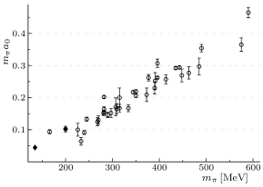
Figure 5: Comparison of the scattering lengths extracted here (filled circle) with various lattice calculations. The filled diamond corresponds to the experimental value determined via Roy equations. The references are given in the main text.

Appendix C Summary of $I=2$ $\pi\pi$ scattering results from lattice QCD

A comparison of the scattering length $a_{0}$ and effective range $r_{0}$ obtained in this work to previous determinations from lattice QCD is shown in Figure 5 and Table 7, respectively. These results do not account for the discretization effects inherent to the different actions used by the various groups. The references are given in the main text.

Appendix D Covariance matrix

All energies and their uncertainties, as well as their normalized covariances, for the single-pion mass, the $I=2$ two-pion spectrum and the $I=3$ three-pion spectrum are given in Table 8. The single-pion mass in the first row is given in lattice units. The scale setting for the D200 ensemble employed here is discussed in Ref. Bruno et al. (2017) of the main text. All other energies are quoted in units of the single-pion mass.

Table 8: Complete spectrum and normalized covariances. Different isospin sectors are separated by large row spacing into $I=1$ (a single pion at rest), $I=2$ and $I=3$. The central values and uncertainties of center-of-mass energies $E_{\mathrm{cm}}/m_{\pi}$ in the second column are measured in units of the pion mass except for the single-pion energy in the first row, which is given in lattice units. The irrep labels are formatted as in Fig. 4.

$A_{1u}^{-}(0)$	.06504(33)	$1$
$A_{1g}^{+}(0)$	2.0172(17)	$-.156$	$1$
	3.715(14)	$-.944$	$.146$	$1$
	4.897(23)	$-.920$	$.179$	$.873$	$1$
$E_{g}^{+}(0)$	3.624(13)	$-.974$	$.194$	$.922$	$.902$	$1$
	4.720(21)	$-.992$	$.147$	$.935$	$.915$	$.962$	$1$
$A_{1}^{+}(1)$	2.4082(41)	$-.796$	$.398$	$.765$	$.741$	$.785$	$.784$	$1$
	4.010(16)	$-.969$	$.190$	$.929$	$.916$	$.947$	$.962$	$.776$	$1$
	4.780(19)	$-.982$	$.167$	$.923$	$.906$	$.958$	$.975$	$.777$	$.951$	$1$
$B_{1}^{+}(1)$	3.889(15)	$-.968$	$.181$	$.919$	$.905$	$.960$	$.959$	$.782$	$.943$	$.957$	$1$
$A_{1}^{+}(2)$	2.6280(49)	$-.837$	$.336$	$.805$	$.780$	$.831$	$.830$	$.725$	$.834$	$.833$	$.831$	$1$
	2.9549(85)	$-.952$	$.191$	$.932$	$.873$	$.934$	$.940$	$.829$	$.926$	$.928$	$.928$	$.828$	$1$
	4.125(16)	$-.991$	$.156$	$.940$	$.916$	$.966$	$.984$	$.791$	$.959$	$.974$	$.961$	$.829$	$.942$	$1$
$A_{2}^{+}(2)$	4.208(16)	$-.993$	$.164$	$.939$	$.914$	$.970$	$.986$	$.793$	$.965$	$.979$	$.967$	$.837$	$.947$	$.985$	$1$
$B_{1}^{+}(2)$	4.091(16)	$-.994$	$.161$	$.940$	$.919$	$.964$	$.988$	$.788$	$.963$	$.978$	$.964$	$.831$	$.945$	$.987$	$.990$	$1$
$A_{1}^{+}(3)$	2.7868(80)	$-.664$	$.276$	$.628$	$.604$	$.661$	$.657$	$.556$	$.678$	$.660$	$.652$	$.635$	$.672$	$.657$	$.671$	$.665$	$1$
	3.344(12)	$-.915$	$.172$	$.896$	$.857$	$.893$	$.905$	$.769$	$.910$	$.904$	$.899$	$.808$	$.913$	$.909$	$.912$	$.906$	$.664$	$1$
$E^{+}(3)$	3.246(10)	$-.971$	$.201$	$.916$	$.896$	$.953$	$.963$	$.774$	$.947$	$.956$	$.948$	$.846$	$.937$	$.965$	$.968$	$.967$	$.687$	$.902$	$1$
$A_{1}^{+}(4)$	2.0133(29)	$-.011$	$.310$	$.048$	$.059$	$.048$	$-.003$	$.144$	$.035$	$.036$	$.076$	$.190$	$.108$	$.027$	$.034$	$.023$	$.104$	$.085$	$.128$	$1$
	2.924(10)	$-.557$	$.215$	$.546$	$.586$	$.570$	$.548$	$.471$	$.565$	$.582$	$.592$	$.524$	$.540$	$.570$	$.567$	$.566$	$.427$	$.539$	$.565$	$.240$	$1$
	3.674(15)	$-.898$	$.164$	$.878$	$.849$	$.887$	$.879$	$.722$	$.890$	$.883$	$.886$	$.796$	$.876$	$.896$	$.895$	$.890$	$.605$	$.859$	$.889$	$.105$	$.547$	$1$
$B_{1}^{+}(4)$	3.628(13)	$-.986$	$.143$	$.932$	$.914$	$.955$	$.988$	$.768$	$.956$	$.972$	$.957$	$.831$	$.933$	$.982$	$.982$	$.985$	$.649$	$.899$	$.961$	$.020$	$.564$	$.883$	$1$
$A_{1u}^{-}(0)$	3.0478(60)	$-.164$	$.813$	$.164$	$.164$	$.182$	$.159$	$.462$	$.180$	$.155$	$.158$	$.268$	$.197$	$.160$	$.162$	$.168$	$.184$	$.172$	$.153$	$.102$	$.083$	$.149$	$.142$	$1$
	4.780(17)	$-.841$	$.130$	$.901$	$.772$	$.829$	$.828$	$.749$	$.831$	$.817$	$.832$	$.717$	$.877$	$.839$	$.843$	$.836$	$.561$	$.818$	$.815$	$.114$	$.516$	$.786$	$.826$	$.157$	$1$
$E_{u}^{-}(0)$	4.691(15)	$-.926$	$.305$	$.887$	$.854$	$.947$	$.915$	$.877$	$.898$	$.908$	$.911$	$.822$	$.930$	$.918$	$.921$	$.917$	$.640$	$.873$	$.909$	$.111$	$.540$	$.848$	$.905$	$.317$	$.846$	$1$
$A_{2}^{-}(1)$	3.5838(85)	$-.606$	$.525$	$.591$	$.571$	$.603$	$.596$	$.907$	$.602$	$.592$	$.602$	$.587$	$.638$	$.600$	$.609$	$.600$	$.385$	$.595$	$.571$	$.135$	$.365$	$.542$	$.576$	$.653$	$.578$	$.717$	$1$
	5.131(18)	$-.916$	$.258$	$.900$	$.853$	$.906$	$.904$	$.825$	$.929$	$.900$	$.902$	$.858$	$.921$	$.903$	$.911$	$.910$	$.677$	$.885$	$.894$	$.111$	$.553$	$.859$	$.897$	$.268$	$.848$	$.911$	$.662$	$1$
$B_{2}^{-}(1)$	5.008(17)	$-.901$	$.271$	$.860$	$.831$	$.900$	$.888$	$.834$	$.877$	$.888$	$.929$	$.849$	$.905$	$.890$	$.897$	$.894$	$.631$	$.857$	$.883$	$.098$	$.548$	$.819$	$.885$	$.285$	$.820$	$.922$	$.691$	$.895$	$1$
$A_{2}^{-}(2)$	3.8840(96)	$-.661$	$.475$	$.654$	$.590$	$.672$	$.647$	$.684$	$.666$	$.649$	$.658$	$.871$	$.702$	$.650$	$.658$	$.656$	$.592$	$.661$	$.678$	$.229$	$.406$	$.620$	$.645$	$.443$	$.602$	$.721$	$.610$	$.751$	$.771$	$1$
	4.206(11)	$-.874$	$.298$	$.861$	$.807$	$.867$	$.860$	$.910$	$.856$	$.849$	$.852$	$.794$	$.937$	$.869$	$.872$	$.868$	$.611$	$.852$	$.861$	$.159$	$.507$	$.817$	$.850$	$.332$	$.852$	$.923$	$.764$	$.899$	$.878$	$.721$	$1$
	5.313(19)	$-.886$	$.233$	$.863$	$.814$	$.887$	$.872$	$.741$	$.878$	$.875$	$.872$	$.812$	$.892$	$.885$	$.886$	$.880$	$.815$	$.883$	$.899$	$.157$	$.530$	$.836$	$.866$	$.174$	$.799$	$.866$	$.540$	$.874$	$.832$	$.694$	$.827$	$1$
$B_{2}^{-}(2)$	5.258(19)	$-.895$	$.233$	$.844$	$.820$	$.887$	$.886$	$.759$	$.888$	$.887$	$.888$	$.810$	$.892$	$.885$	$.894$	$.899$	$.817$	$.874$	$.900$	$.128$	$.549$	$.823$	$.879$	$.191$	$.786$	$.876$	$.562$	$.874$	$.865$	$.703$	$.841$	$.915$	$1$
$A_{2}^{-}(3)$	4.088(18)	$-.416$	$.348$	$.376$	$.365$	$.420$	$.406$	$.445$	$.415$	$.415$	$.427$	$.430$	$.413$	$.398$	$.421$	$.417$	$.624$	$.399$	$.413$	$.121$	$.252$	$.356$	$.393$	$.351$	$.369$	$.453$	$.398$	$.475$	$.476$	$.457$	$.389$	$.492$	$.518$	$1$
	4.608(14)	$-.840$	$.253$	$.827$	$.769$	$.830$	$.826$	$.775$	$.818$	$.829$	$.831$	$.822$	$.881$	$.827$	$.833$	$.830$	$.646$	$.904$	$.834$	$.139$	$.519$	$.796$	$.819$	$.262$	$.790$	$.861$	$.628$	$.877$	$.870$	$.766$	$.845$	$.840$	$.834$	$.475$	$1$
	4.850(17)	$-.914$	$.176$	$.905$	$.840$	$.898$	$.903$	$.817$	$.891$	$.893$	$.892$	$.810$	$.967$	$.906$	$.913$	$.908$	$.639$	$.902$	$.900$	$.144$	$.533$	$.843$	$.895$	$.181$	$.867$	$.903$	$.626$	$.903$	$.879$	$.693$	$.927$	$.866$	$.862$	$.396$	$.870$	$1$
$E^{-}(3)$	4.528(14)	$-.826$	$.281$	$.794$	$.742$	$.814$	$.807$	$.817$	$.798$	$.805$	$.809$	$.797$	$.841$	$.814$	$.817$	$.824$	$.631$	$.792$	$.836$	$.125$	$.455$	$.760$	$.800$	$.330$	$.750$	$.853$	$.686$	$.832$	$.863$	$.777$	$.835$	$.788$	$.806$	$.481$	$.844$	$.825$	$1$