Revealing mass-degenerate states in Higgs boson signals

Abstract

The observed Higgs boson signals to-date could be due to having two quasi-degenerate $125\>\text{GeV}$ scalar states in Nature. This kind of scenario tallies well with the predictions from the Next-to-Minimal Supersymmetric Standard Model (NMSSM). We have analysed the phenomenological NMSSM Higgs boson couplings and derived a parameterization of the signal strengths within the two quasi-degenerate framework. With essentially two parameters, it is shown that the combined strengths of the two quasi-degenerate Higgs states in the leptonic (and b-quark) decay channels depart from the Standard Model values in the opposite direction to those in the vector boson channels. We identify experimental measurements for distinguishing a single from a double Higgs scenarios. The proposed parameterization can be used for benchmarking studies towards establishing the status of quasi-degenerate Higgs scenarios.

1 Introduction

Higgs boson discovery represents the beginning of a new epoch for fundamental physics. The precise measurements of its couplings is an important aim for particle physics which could possibly give hint to physics beyond the Standard Model. With current data, the Higgs properties are compatible with the prediction of the Standard Model [1, 2]. These same properties could also be due to the combination of effects arising from having two quasi-degenerate scalar states around $125\>\text{GeV}$. Such a tantalizing possibility have been predicted by new physics models such as the Next-to Minimal Supersymmetric Standard Model (NMSSM). The impact of the Higgs properties and precision measurements on the NMSSM scenarios with two quasi-degenerate scalars will contribute towards sharpening our understanding of the Higgs boson data and Nature – it could be that the data might have already contain some indications for new physics.

The current state of findings from the Large Hadron Collider (LHC), i.e. the absence of direct signals of physics beyond the Standard Model (BSM), has been forecasted for the case of supersymmetry (SUSY) by pre-LHC global fits of models to data. For instance, as pointed out in [3, 4, 5] the large mass of the Higgs was already an indication for heavy supersymmetric mass spectra. Within such models, phenomenological studies could be done via two main approaches, namely the simplified models approach [6, 7] and the phenomenological model parameterization [8, 9, 10, 5, 11]. In this article, the latter approach will be used.

Several groups have addressed mass-degenerate Higgs scenarios within the NMSSM. Refs. [12, 13, 14] have considered two quasi-degenerate Higgs states for the real and complex NMSSM, with a mass difference large enough to use the narrow width approximation. Ref. [15] has gone beyond the narrow width approximation and showed that interference effects can account for up to 40% of total cross sections. To be able to conclude that departures from SM prediction are a consequence of the existence of more than one resonance [16, 17] have proposed statistical test based on the analysis of a signal strength matrix, where all the channels are considered independent. A simplified version of their results agrees with what was proposed previously in [12]. In this article, we focus on the possibility of having two mass-degenerate states with different coupling structures that when combined mimic a single Higgs features. The main aim is to derive a set of NMSSM parameters most relevant for quasi-degenerate Higgs studies vis-á-vise collider data. For this, the NMSSM doublet-singlet mixings structure [18, 19, 15] of the Higgs sector will be used.

In section 2 we review the production and decay ratios of the two lightest NMSSM CP-even Higgs states. We focus on the couplings of these to vector bosons and heavy quarks. In section 3 we perform a scan of the parameters of the NMSSM while imposing that the the two lightest CP-even Higgs states reproduce the mass of the standard Higgs measured by the LHC. We describe the allowed parameter space regions and relevant parameter correlations. In section 4 the sample is then used together with analytical relations for the couplings and signal strengths to show that the the quasi-degenerate Higgs properties can be explained approximately by using just two free parameters. We also we show how the superposition of two quasi-degenerate Higgs around 125 GeV could be in agreement with current experimental results. Finally in section 5 we analyse the sample based on signal strength ratios that can discriminate between the single versus double resonance scenarios.

2 Higgs couplings to fermions and vector bosons

Right after the discovery of the Higgs the search for signals of physics beyond Standard Model in the production and decay of the Higgs became a priority. A possible excess in the $\gamma\gamma$ channel motivated a lot of work, some of them within the NMSSM framework [20, 21, 12, 19, 22]. In particular King et. al. [19] pointed out that the signal strengths of the $\gamma\gamma$ channels could be enhanced for large singlet-double mixing. We will take these as a starting point for analysing two quasi-degenerate CP-even Higgs states.

For the discussion of the following sections it is important to have a clear picture of how the widths and therefore the Higgs branching ratios depend on the singlet-doublet mixing. Let us start introducing some notation, we define $\psi=(H_{d},H_{u},s)$ and $\phi=(h_{0},H_{0},s)$ in such a way that $\langle h_{0}\rangle=v$ and $\langle H_{0}\rangle=0$:

$$\phi_{i}=N_{ij}\psi_{j}$$ (1)

where

$$N=\left(\begin{array}[h]{ccc}\cos\beta&\sin\beta&0\\ \sin\beta&-\cos\beta&0\\ 0&0&1\end{array}\right).$$ (5)

The Higgs states $h=(h_{1},h_{2},h_{3})$ are related to $\psi$ and $\phi$ in the following way,

$$h_{i}=U_{ij}\phi_{j}$$ (6)

where $U_{ij}$ are the elements of the mixing matrix, $U$. We consider it convenient to use the elements of $U$ to parameterise the couplings; for example $U_{i1}$ and $U_{i2}$ are respectively the $h_{0}$-component and $H_{0}$-component of $h_{i}$. In this way it is easier to make the comparison to the standard Higgs.

Using the above notation we write the tree-level Higgs couplings to vector bosons and heavy quarks as:

$$g_{h_{i}ZZ} = g_{\mu\nu}\frac{g_{1}^{2}+g_{2}^{2}}{\sqrt{2}}\,v^{2}\,U_{i1},$$

$$g_{h_{i}WW} = g_{\mu\nu}\frac{g_{2}^{2}}{\sqrt{2}}\,v^{2}\,U_{i1},$$

$$g_{h_{i}tt} = \frac{m_{t}}{\sqrt{2}v}[\,U_{i1}-\cot\beta\,U_{i2}\,],$$

$$g_{h_{i}bb} = \frac{m_{b}}{\sqrt{2}v}[\,U_{i1}+\tan\beta\,U_{i2}\,].$$ (7)

In the $H_{0}$ decoupling limit (i.e. $U_{12}=U_{22}=0$) all the couplings are proportional to $U_{11}$, the $h_{0}$-component of $h_{1}$. We are interested in the departure of the production and decay signals of $h_{1}$ in the $Z_{3}$-invariant NMSSM with respect to the one of the standard Higgs. To weight this we will use the signal strength,

$$\mu=\frac{\sigma(SM\rightarrow h_{i}\rightarrow SM)|_{NMSSM}}{\sigma(SM\rightarrow h_{SM}\rightarrow SM)|_{SM}}$$ (8)

Because of the small width of the Higgs states we assume they are produced on-shell, therefore the total cross sections are evaluated as the production cross section times the branching ratio.

Now, in order to obtain the required properties for the Higgs states to reproduce ATLAS and CMS measurements we consider two possibilities:

1. $h_{1}$ or $h_{2}$ is the Higgs state detected at the LHC, and

2. $h_{1}$ and $h_{2}$ are the Higgs states measured by the LHC, where $h_{1}$ and $h_{2}$ are mass degenerate.

We will show that these two possibilities correspond, respectively, to:

1. Small singlet-doublet mixing, and

2. Large singlet-doublet mixing.

Let us analyse the case with small singlet-doublet mixing where $h_{1}$ is mainly $h_{0}$, in other words $U_{11}\sim 1$. For this case it is a good approximation to consider that the width of $h_{1}$ is dominated by the decay rate of $h_{1}\rightarrow b\bar{b}$ and therefore the variation of the width is controlled by the square of the Higgs coupling to bottom quarks, $g_{h_{1}b\bar{b}}$. Using the couplings described in eq. (2) the signal strengths of the vector-boson fusion production of $h_{1}$ and further decay to $WW/ZZ$ and $b\bar{b}$ are approximately,

$$\mu_{\mathrm{VBF}\rightarrow h_{1}\rightarrow\mathrm{WW/ZZ}} \simeq \hat{g}_{h_{1}WW}^{2}\frac{\hat{g}_{h_{1}WW}^{2}}{\hat{g}_{h_{1}bb}^{2}}=[U_{11}]^{2}\ \frac{[U_{11}]^{2}}{[U_{11}+\tan\beta\,U_{12}]^{2}},$$ (9)

$$\mu_{\mathrm{VBF}\rightarrow h_{1}\rightarrow b\bar{b}} \simeq \hat{g}_{h_{1}WW}^{2}\frac{\hat{g}_{h_{1}bb}^{2}}{\hat{g}_{h_{1}bb}^{2}}=[U_{11}]^{2},$$ (10)

where $\hat{g}=g_{\mathrm{NMSSM}}/g_{\mathrm{SM}}$, the couplings $g_{\mathrm{NMSSM}}$ are those in eq. (2), and $g_{\mathrm{SM}}$ are the Standard Model (SM) couplings. The enhancement or suppression of the first signal strengths depends on $\tan\beta\,\,U_{12}/U_{11}$. As such, the absolute value and sign of this factor determines respectively the magnitude of the ratio between the signal strengths and whether there is an enhancement or suppression of $\mu_{\mathrm{VBF}\rightarrow h_{1}\rightarrow\mathrm{WW/ZZ}}$ with respect to $\mu_{\mathrm{VBF}\rightarrow h_{1}\rightarrow b\bar{b}}$. A similar analysis holds when $h_{2}$ is considered the Higgs state measured at the LHC.

Next, let us examine the case with large singlet-doublet mixing where $h_{1}$ has non-negligible S content. In this case, the approximation $U_{11}\sim 1$ is not valid any more. The assumption that the width of $h_{1}$ is almost totally controlled by $h_{1}\rightarrow b\bar{b}$ is no longer a good approximation. The size of $\tan\beta\,U_{12}/U_{11}$ may take very large values and therefore the branching ratio could significantly differ with respect to the standard Higgs. So, we would like to have a simple expression for the widths appropriate for all values of $U_{i1}$. In terms of the standard Higgs decay rates, one can write

$$\Gamma_{i} = \Gamma_{h_{i}\rightarrow bb/\tau\tau}+\Gamma_{h_{i}\rightarrow WW/ZZ}+\Gamma_{h_{i}\rightarrow SM_{\mathrm{rest}}}$$ (11)

$$= \hat{g}_{h_{i}bb/\tau\tau}^{2}\,\Gamma_{(h_{SM}\rightarrow bb/\tau\tau)}\,+\hat{g}_{h_{i}WW/ZZ}^{2}\,\Gamma_{(h_{SM}\rightarrow WW/ZZ)}\,+(U_{i1})^{2}\,\Gamma_{(h_{SM}\rightarrow SM_{\mathrm{rest}})}$$ (12)

where $h_{i}\rightarrow\mathrm{SM}_{\mathrm{rest}}$ represents the rest of the decay channels. The dominant contribution for the rest of decay channels is the decay to gluons through a top loop. For simplicity we are going to consider that the rest of the decay modes behave as the ones of the standard Higgs. For this reason we took the corresponding decay rate proportional to the square of $h_{i}$’s $h_{0}$ content, $U_{i1}$. By writing the decay rates in terms of the SM branching ratios we get

$$\Gamma_{i}/\Gamma_{\mathrm{SM}} \simeq \mathrm{BR}_{h_{SM}\rightarrow bb/\tau\tau}\,\hat{g}_{h_{i}bb/\tau\tau}^{2}+\mathrm{BR}_{h_{SM}\rightarrow WW/ZZ}\,\hat{g}_{h_{i}WW/ZZ}^{2}+\mathrm{BR}_{h_{SM}\rightarrow SM}\,(U_{i1})^{2}$$ (13)

$$\simeq \mathrm{BR}_{h_{SM}\rightarrow bb/\tau\tau}(U_{i1}+U_{i2}\tan\beta)^{2}+(1-\mathrm{BR}_{h_{SM}\rightarrow bb/\tau\tau})(U_{i1})^{2}.$$ (14)

For large singlet-doublet mixing the widths of $h_{1}$ and $h_{2}$ could be much smaller than $\Gamma_{\mathrm{SM}}$, producing large departures of the branching ratios with respect to the ones of the standard Higgs, unless the widths and the decay rates of each Higgs state change at the same proportion. From now on we will use eq. (13) as the enhancement(suppression) rate of the width with respect to the SM value.

The analytic expressions for the signal strengths for vector-boson fusion production and decay to $WW/ZZ$ and $b\bar{b}$ can be written as,

$$\mu_{VBF\rightarrow h_{1}\rightarrow WW/ZZ}^{\mathrm{an}} \simeq \frac{(U_{11})^{4}}{(1-\mathrm{BR}_{h_{SM}\rightarrow bb/\tau\tau})(U_{11})^{2}+\mathrm{BR}_{h_{SM}\rightarrow bb/\tau\tau}(U_{11}+U_{12}\tan\beta)^{2}},$$ (15)

$$\mu_{VBF\rightarrow h_{2}\rightarrow WW/ZZ}^{\mathrm{an}} \simeq \frac{(U_{21})^{4}}{(1-\mathrm{BR}_{h_{SM}\rightarrow bb/\tau\tau})(U_{21})^{2}+\mathrm{BR}_{h_{SM}\rightarrow bb/\tau\tau}(U_{21}+U_{22}\tan\beta)^{2}},$$ (16)

$$\mu_{VBF\rightarrow h_{1}\rightarrow bb}^{\mathrm{an}} \simeq \frac{(U_{11})^{2}(U_{11}+\tan\beta U_{12})^{2}}{(1-\mathrm{BR}_{h_{SM}\rightarrow bb/\tau\tau})(U_{11})^{2}+\mathrm{BR}_{h_{SM}\rightarrow bb/\tau\tau}(U_{11}+U_{12}\tan\beta)^{2}},$$ (17)

$$\text{ and }\mu_{VBF\rightarrow h_{2}\rightarrow bb}^{\mathrm{an}} \simeq \frac{(U_{21})^{2}(U_{21}+\tan\beta U_{22})^{2}}{(1-\mathrm{BR}_{h_{SM}\rightarrow bb/\tau\tau})(U_{21})^{2}+\mathrm{BR}_{h_{SM}\rightarrow bb/\tau\tau}(U_{21}+U_{22}\tan\beta)^{2}}.$$ (18)

Note that for a large singlet-doublet mixing the relative size of $\tan\beta\,U_{12}/U_{11}$ has a larger range of variation than in the case of small singlet-doublet mixing, as consequence there might be larger enhancement(suppression) to the signals. Moreover, since the $H_{0}$-component of the Higgs states is the one responsible for large variations of the branching ratios, it is interesting to see that in the $H_{0}$ decoupling limit ($U_{12}\simeq 0$ and $U_{22}\simeq 0$),

$$\lim_{m_{H_{0}}\gg\,m_{h_{0}},m_{S}}\mu_{VBF\rightarrow h_{i}\rightarrow WW/ZZ}^{\mathrm{an}}\simeq(U_{i1})^{2}\ \ ,\textrm{ and }\qquad\lim_{m_{H_{0}}\gg\,m_{h_{0}},m_{S}}\mu_{VBF\rightarrow h_{i}\rightarrow bb}^{\mathrm{an}}\simeq(U_{i1})^{2}.$$

Hence for large singlet-doublet mixing it is not possible to reproduce the experimental data with a single Higgs state. But, if $h_{1}$ and $h_{2}$ are mass quasi-degenerate, assumed to be unresolved away from each other by experiments, the superposition of the two states could show up in signals as single standard Higgs with,

$$\lim_{m_{H_{0}}\gg m_{h_{0}},m_{S}}\mu_{VBF\rightarrow h_{1}\rightarrow WW/ZZ}^{\mathrm{an}}+\mu_{VBF\rightarrow h_{2}\rightarrow WW/ZZ}^{\mathrm{an}}\simeq(U_{11})^{2}+(U_{21})^{2}\sim 1\textrm{ and }$$ (19)

$$\lim_{m_{H_{0}}\gg m_{h_{0}},m_{S}}\mu_{VBF\rightarrow h_{1}\rightarrow bb}^{\mathrm{an}}+\mu_{VBF\rightarrow h_{2}\rightarrow bb}^{\mathrm{an}}\simeq(U_{11})^{2}+(U_{21})^{2}\sim 1.$$ (20)

Notice that the last (approximate)equalities require $U_{31}\simeq 0$ to fulfill the unitarity condition for U.

It is interesting to compare the departure of the signal strengths for different channels of the same Higgs state. As described earlier, the ratio between signal strengths depends on $\tan\beta\,U_{12}/U_{11}$ for $h_{1}$ and on $\tan\beta\,U_{22}/U_{21}$ for $h_{2}$. As such, the departure of the global signal strength will depend on the relation between $U_{12}$ and $U_{22}$.

In the following sections we analyse the scenario with large singlet-doublet mixing. We will assume that the Higgs signal measured by ATLAS and CMS is a superposition of the production and decay of two Higgs states. To get the global enhancement(suppression) we will sum the contribution of the two Higgs states. Notice that for this approximation to be valid the widths should be much smaller that the mass difference between $h_{2}$ and $h_{1}$.

3 The phenomenological NMSSM Parameters scan

Let us consider the case where the Higgs signal measured by ATLAS and CMS is a superposition of the production and decay of $h_{1}$ and $h_{2}$, meaning that the Higgs states are close enough not to be resolved by the experiments, but with large enough separation to have negligible interference effects. To study the region of the parameter space of the NMSSM where this condition is fulfilled we perform a parameter scan as done in [23].

3.1 The phenomenological NMSSM (pNMSSM)

We shall consider an R-parity conserving NMSSM with superpotential,

$$W_{NMSSM}=W_{MSSM^{\prime}}-\epsilon_{ab}\lambda{S}{H}^{a}_{1}{H}^{b}_{2}+\frac{1}{3}\kappa{S}^{3}\ ,$$ (21)

where

$$W_{MSSM^{\prime}} = \epsilon_{ab}\left[(Y_{E})_{ij}H_{1}^{a}L_{i}^{b}{\bar{E}}_{j}+(Y_{D})_{ij}H_{1}^{a}Q_{i}^{b}{\bar{D}}_{j}+(Y_{U})_{ij}H_{2}^{b}Q_{i}^{a}{\bar{U}}_{j}\right].$$ (22)

The chiral superfields have the following $SU(3)_{C}\otimes SU(2)_{L}\otimes U(1)_{Y}$ quantum numbers,

$$L:(1,2,-\frac{1}{2}),\quad{\bar{E}}:(1,1,1),$$ (23)

$$Q:\,(3,2,\frac{1}{6}),\quad{\bar{U}}:\,(\bar{3},1,-\frac{2}{3}),\quad{\bar{D}}:(\bar{3},1,\frac{1}{3}),$$ (24)

$$H_{1}:(1,2,-\frac{1}{2}),\quad H_{2}:\,(1,2,\frac{1}{2}).$$ (25)

The corresponding soft SUSY-breaking terms are

$$V_{\mathrm{soft}}=V_{2}+V_{3}+m_{\mathrm{S}}^{2}|S|^{2}+(-\epsilon_{ab}\lambda A_{\lambda}{S}{H}^{a}_{1}{H}^{b}_{2}+\frac{1}{3}\kappa A_{\kappa}{S}^{3}+\mathrm{H.c.}),$$ (26)

with

$$V_{2} = m_{H_{1}}^{2}{{H^{*}_{1}}_{a}}{H_{1}^{a}}+m_{H_{2}}^{2}{{H^{*}_{2}}_{a}}{H_{2}^{a}}+{\tilde{Q}^{*}}_{i_{L}a}(m_{\tilde{Q}}^{2})_{ij}\tilde{Q}_{j_{L}}^{a}+{\tilde{L}^{*}}_{i_{L}a}(m_{\tilde{L}}^{2})_{ij}\tilde{L}_{j_{L}}^{a}+$$ (27)

$$\tilde{u}_{i_{R}}(m_{\tilde{u}}^{2})_{ij}{\tilde{u}^{*}}_{j_{R}}+\tilde{d}_{i_{R}}(m_{\tilde{d}}^{2})_{ij}{\tilde{d}^{*}}_{j_{R}}+\tilde{e}_{i_{R}}(m_{\tilde{e}}^{2})_{ij}{\tilde{e}^{*}}_{j_{R}},$$

$$V_{3} = \epsilon_{ab}\sum_{ij}\left[(T_{E})_{ij}H_{1}^{a}\tilde{L}_{i_{L}}^{b}\tilde{e}_{j_{R}}^{*}+(T_{D})_{ij}H_{1}^{a}\tilde{Q}_{i_{L}}^{b}\tilde{d}_{j_{R}}^{*}+(T_{U})_{ij}H_{2}^{b}\tilde{Q}_{i_{L}}^{a}\tilde{u}_{j_{R}}^{*}\right]+\mathrm{H.c.}.$$ (28)

A tilde-sign over the superfield symbol represents the scalar component. However, an asterisk over the superfields as in, for example, $\tilde{u}_{R}^{*}$ represents the scalar component of $\bar{U}$. The $SU(2)_{L}$ fundamental representation indices are donated by $a,b=1,2$ while the generation indices by $i,j=1,2,3$. $\epsilon_{12}=\epsilon^{12}=1$ is a totally antisymmetric tensor.

In an approach similar to that of the pMSSM [8, 9, 10, 5], the pNMSSM parameters are defined at the weak scale with the non-Higgs sector set,

$$M_{1,2,3};\;\;m^{3rd\,gen}_{\tilde{f}_{Q,U,D,L,E}},\;\;m^{1st/2nd\,gen}_{\tilde{f}_{Q,U,D,L,E}};\;\;A_{t,b,\tau}.$$ (29)

Here, $M_{1,2,3}$ and $m_{\tilde{f}}$ are respectively the gaugino and the sfermion mass parameters. $A_{t,b,\tau}$ represent the trilinear scalar couplings. With electroweak symmetry breaking,an effective $\mu$-term, $\mu_{\mathrm{eff}}=\lambda\,v_{s}$ is developed. The $\mu$-term, the ratio of the MSSM-like Higgs doublets’ vevs $\tan\beta=\left<H_{2}\right>/\left<H_{1}\right>$ and the Z-boson mass, $m_{Z}$ lead to the tree-level Higgs sector parameters

$$\tan\beta,\lambda,\kappa,A_{\lambda},A_{\kappa},\lambda\,v_{s}.$$ (30)

Next, including four SM nuisance parameters, namely, the top and bottom quarks $m_{t,b}$, $m_{Z}$ and the strong coupling constant, $\alpha_{s}$, makes the pNMSSM parameters:

$$\theta=\{M_{1,2,3};\;\;m^{3rd\,gen}_{\tilde{f}_{Q,U,D,L,E}},\;\;m^{1st/2nd\,gen}_{\tilde{f}_{Q,U,D,L,E}};\;\;A_{t,b,\tau,\lambda,\kappa};\;\;\tan\beta,\lambda,\kappa,\mu_{\mathrm{eff}};\;\;m_{t,Z,b},\alpha_{s}\}.$$ (31)

3.2 The scanning procedure

$M_{1,2}$ affects the gaugino masses for which a wide range, $\mathcal{O}(\mathrm{GeV})$ to $\mathcal{O}(\mathrm{TeV})$, is possible. We let $M_{1}\in[-4,4]\>\text{TeV}$ and same for $M_{2}>0$. With the LHC in mind, we let the gluino and squark mass parameters be within $[100\>\text{GeV},4\>\text{TeV}]$, and the trilinear scalar couplings allowed in $[-8\>\text{TeV},8\>\text{TeV}]$. $\tan\beta$ is allowed between 2 and 60. For minimising fine-tuning, we subjectively let $\mu_{\mathrm{eff}}=\lambda\,v_{s}$ to vary within 100 to 400 GeV not too far away from the Z-boson mass. The remaining Higgs-sector parameters were set within the ranges shown in Table 1.

Parameter	Range	Posterior range
$M_{1}$	[$-4$ TeV, $4$ TeV]
$M_{2}$	[$0$ TeV, $4$ TeV]
$M_{3},\,\,m^{3rd\,gen,\,\,1st/2nd\,gen}_{\tilde{f}_{Q,U,D,L,E}}$	[$100$ GeV, $4$ TeV]
$A_{t,b,\tau}$	[-$8$ TeV, $8$ TeV]
$\tan\beta$	[$2$, $60$]	[$8.8$, $28.3$]
$\lambda$	[$10^{-4}$, $0.75$]	[$0.17$, $0.52$]
$\kappa$	[$-0.75$, $0.75$]	[$-0.50$, $0.75$]
$\mu_{\mathrm{eff}}$	[$100$, $400$] GeV	[$111$, $308$] GeV
$A_{\lambda}$	[$50$ GeV, $4$ TeV]	[$1.34$, $4$] TeV
$A_{\kappa}$	[$-2$ TeV, $2$ TeV]	[$-1646$, $846$] GeV
$m_{t}$	172.6 $\pm$ 1.4 GeV
$m_{Z}$	91.1876 $\pm$ 0.0021 GeV
$m_{b}(m_{b})^{\overline{MS}}$	4.20 $\pm$ 0.07 GeV
$\alpha_{s}(m_{Z})^{\overline{MS}}$	0.1172 $\pm$ 0.002

Table 1: The 26 pNMSSM parameters and their corresponding flat prior probability density distribution ranges. The SM parameters were varied according to Gaussian distributions with the shown central values and standard deviations. The third column (to be addressed in section. 4) shows the 95% Bayesian confidence regions for the posterior sample used in Figure. 4. For this posterior sample, $m_{h_{2}}-m_{h_{1}}<3$ GeV with both $m_{h_{1}}$ and $m_{h_{2}}$ allowed within [$122$, $128$] GeV.

The selected pNMSSM points were required pass all the constraints summarised in Tab.2. These are: the Higgs boson mass $m_{h}$, the neutralino cold dark matter (CDM) relic density $\Omega_{CDM}h^{2}$, anomalous magnetic moment of the muon $\delta a_{\mu}$, and the B-physics related limits summarised in the upper part of Table 2. The experimental constraints used were those implemented in NMSSMTools [24, 25, 26, 27, 28, 29], Lilith [30], MicrOMEGAs [31, 32, 33, 34, 35, 36, 37, 38, 39, 40], SModelS’[41, 42, 43, 44, 45, 46, 47, 48, 49, 50, 51] implementation of ATLAS and CMS limits[52, 53, 54, 55, 56, 57, 58, 59, 60, 61, 62], and HiggsBounds [63, 64, 65, 66, 67, 68, 69, 70, 71, 72, 73, 74, 75, 76, 77]. The Higgs boson signal strength measurements from Tevatron [78], ATLAS [2, 79, 80, 81, 82, 83, 84, 85, 69, 86, 67] and CMS [74, 75, 76, 87, 88, 89, 90, 91, 92, 93, 68] as implemented in Lilith v1.1 (with data version 15.09) [30] were also included.

Observable	Constraint	References
$m_{h}$	$125.09\pm 3.0$ GeV	[94]
$Br(B\rightarrow X_{s}\gamma)$	$(3.32\pm 0.16)\times 10^{4}$	[95, 96, 97]
$Br(B_{s}\rightarrow\mu^{+}\mu^{-})$	$(3.0\pm 0.6)\times 10^{-9}$	[98, 99, 100]
$\Delta M_{B_{s}}$	$17.757\pm 0.021$	[100, 101]
$\Delta M_{B_{d}}$	$0.5064\pm 0.0019$	[100, 101]
$Br(B_{u}\rightarrow\tau\nu)$	$1.06\pm 0.19$	[102, 103, 104, 105]
$\delta a_{\mu}$	$(30.2\pm 8.80)\times 10^{-10}$	[106, 28, 29]
$\Omega_{CDM}h^{2}$	$0.12\pm 0.02$	[107]
Higgs signal strengths		[78, 2, 79, 80, 81, 82, 83, 84, 85, 69, 86, 67, 74, 75, 76, 87, 88, 89, 90, 91, 92, 93, 68]
CDM direct detection limits		[108, 109, 110, 111, 112, 113, 114]
Constraints in HiggsBounds		[63, 64, 65, 66, 67, 68, 69, 70, 71, 72, 73, 74, 75, 76, 77]
Constraints in SModelS		[41, 42, 43, 44, 45, 46, 47, 48, 49, 50, 51, 52, 53, 54, 55, 56, 57, 58, 59, 60, 61, 62]

Table 2: Summary of the central values and errors for the observables. Theoretical uncertainties have been added in quadrature to the experimental uncertainties quoted.

3.3 Constraints on the parameters of the Higgs sector

From the pNMSSM parameter scan, we use a sample with two quasi-degenerate lightest CP-even Higgs bosons. It was required that $h_{1}$ and $h_{2}$ have mass equal to $125\pm 3$ GeV, where the $\pm 3$ GeV accounts to the theoretical errors associated to the values of the masses computed by NMSSMtools. In addition it was required that the mass difference, $m_{h_{2}}-m_{h_{1}}<3$ GeV . We focus on the regions of the Higgs sector parameters for studying the correlations within those parameters and for relating them to other parameters which are directly connected with the signals measured at the LHC such as the CP-even Higgs mixing matrices.

It is useful to have an explicit form for the Higgs mixing matrix $U$. We parameterise this using three angles $\theta_{13}$, $\theta_{12}$, and $\theta_{23}$ such that

$$U = \left(\begin{array}[h]{ccc}c_{13}&0&s_{13}\\ -s_{13}&0&c_{13}\\ 0&1&0\end{array}\right)\left(\begin{array}[h]{ccc}1&0&0\\ 0&c_{23}&s_{23}\\ 0&-s_{23}&c_{23}\end{array}\right)\left(\begin{array}[h]{ccc}c_{12}&s_{12}&0\\ -s_{12}&c_{12}&0\\ 0&0&1\end{array}\right)$$ (41)

$$= \left(\begin{array}[h]{ccc}c_{13}c_{12}+s_{13}s_{23}s_{12}&c_{13}s_{12}-s_{13}s_{23}c_{12}&s_{13}c_{23}\\ -s_{13}c_{12}+c_{13}s_{23}s_{12}&-s_{13}s_{12}-c_{13}s_{23}c_{12}&c_{13}c_{23}\\ -c_{23}s_{12}&c_{23}c_{12}&s_{23}\end{array}\right).$$ (45)

Here $c_{ij}=\cos\theta_{ij}$ and $s_{ij}=\sin\theta_{ij}$. Given the mixing matrix, obtained numerically by the SUSY spectra calculator NMSSMtools, then the mixing angles can be extracted as:

$$s_{23}=U_{33},\quad \quad s_{13}=\frac{U_{13}}{c_{23}},$$ (46)

$$s_{12}=-\frac{U_{31}}{c_{23}},\quad \quad c_{13}=\frac{U_{23}}{c_{23}}.$$ (47)

Now, considering that we want to reproduce a standard Higgs signal, we determine the expected ranges for the mixing angles. In order to get the ratio between $\mu_{VBF\rightarrow h_{1,2}\rightarrow WW/ZZ}$ and $\mu_{VBF\rightarrow h_{1,2}\rightarrow bb}$ close to one, either the value of $\mu_{VBF\rightarrow h_{i}\rightarrow WW/ZZ}/\mu_{VBF\rightarrow h_{i}\rightarrow bb}$ for each Higgs state has to be close to one, or a fine cancellation should take place. In this work we focus on the first case. From eqs. (15)-(18) one can see that this condition is possible when $U_{12}$ and $U_{22}$ are very small and as a result $s_{12}$ and $s_{23}$ should also be very small according to eq. (41). On an other hand, eq. (19) implies that the superposition of $h_{1}$ and $h_{2}$ can reproduce the standard Higgs signal for $U_{31}\sim 0$ (i.e. large values of $m_{H_{0}}$). For this to happen either $\theta_{12}$ has to be very small or $\theta_{23}$ has to be close to $\pm\pi/2$. In summary, $\theta_{12}\sim 0$ and $\theta_{23}\sim 0$ will guarantee that we are working in the regime where the superposition of the two Higgs states agrees with experimental measurements.

In the limit of small $\theta_{12}$ and $\theta_{23}$,

$$s_{12}\simeq\theta_{12},\quad s_{23}\simeq\theta_{23},\quad c_{12}\simeq 1,\quad c_{23}\simeq 1$$

and the mixing matrix eq. (41) reduces to

$$U \simeq \left(\begin{array}[h]{ccc}c_{13}&c_{13}\theta_{12}-s_{13}\theta_{23}&s_{13}\\ -s_{13}&-s_{13}\theta_{12}-c_{13}\theta_{23}&c_{13}\\ -\theta_{12}&1&\theta_{23}\end{array}\right)$$ (51)

where we have neglected $\mathcal{O}(\theta^{2})$ terms. For the results of our scan this approximation works with a $0.5\%$ error.

We have been able to constrain the parameters of the mixing matrix requiring conditions that will give us a standard-like Higgs signal. This conditions will affect the masses or couplings of the heaviest and pseudoscalar Higgs bosons. To see this, it will be useful to relate the mixing angles $\theta_{13}$, $\theta_{23}$ and $\theta_{12}$ to the fundamental parameters of the Higgs sector. Using eq. (41) we relate the terms of the mass matrix with the physical masses by introducing two new parameters: $m_{h}^{2}$, the central value of the two lightest CP-even Higgs states, and $\delta m_{h}^{2}$, half of the squared mass difference,

$$U^{T}\,\mathcal{M}\,U=\mathrm{diag}\{m_{h}^{2}-\delta m_{h}^{2},\ m_{h}^{2}+\delta m_{h}^{2},\ m_{h_{3}}^{2}\}.$$ (52)

To simplify the expressions obtained from eq. (52) we factorise $c_{12}$ and $c_{23}$ to write U in terms of $t_{kl}\equiv\tan\theta_{kl}$ and use the approximations:

$$c_{12}\simeq 1,\qquad c_{23}\simeq 1,\qquad\frac{1}{2}\pm\tan\theta_{kl}\tan\theta_{mn}\simeq\frac{1}{2},$$ (53)

where $kl=12,23$ and $mn=12,23$. Finally, we will focus on the relations in terms of the mass matrix elements $\mathcal{M}_{22}$ and $\mathcal{M}_{23}$ since $\mathcal{M}_{22}^{\mathrm{tree}}$ and $\mathcal{M}_{23}^{\mathrm{tree}}$ reproduce pretty well the values computed by NMSSMtools, and because we wish to get simple relations between the Higgs sector parameters, masses and mixing angles. We have checked numerically that for the rest of mass matrix elements the tree level expression are not precise enough.

$$\mathcal{M}_{22}-m_{h_{3}}^{2} = m_{h}^{2}\left(t_{23}^{2}+t_{12}^{2}\right)+\cos(2\theta_{13})\,\delta m_{h}^{2}\left(t_{23}^{2}-t_{12}^{2}\right)+2\sin(2\theta_{13})\,\delta m_{h}^{2}t_{12}\,t_{23}$$ (54)

$$\mathcal{M}_{13}+\mathcal{M}_{23}\,t_{12} = -\sin(2\theta_{13})\,\delta m_{h}^{2}$$ (55)

$$\mathcal{M}_{22}\,t_{23}-\mathcal{M}_{23} = m_{h}^{2}t_{23}+\delta m_{h}^{2}\left[\,t_{12}\sin(2\theta_{13})+t_{23}\cos(2\theta_{13})\,\right].$$ (56)

We can further simplify eq. (54) taking into account that $\delta m_{h}^{2}$ and $m_{h}^{2}$ are smaller than $m_{h_{3}}$ and $\mathcal{M}_{22}$. Using the last approximation of eq. (53) we get that terms proportional to $t_{12}^{2}$, $t_{23}^{2}$ and $t_{12}t_{23}$ in the right hand of eq. (54) are negligible. Regarding eq. (56), using the approximation eq. (53) and eq. (55) one gets $\mathcal{M}_{23}+\delta m_{h}^{2}\,t_{12}\sin(2\theta_{13})\simeq\mathcal{M}_{23}$, allowing us to neglect the term proportional to $t_{12}$ in eq. (56) (besides that, for the sample of pNMSSM points described in section 3 the values of $\theta_{12}$ are much smaller than the values of $\theta_{23}$). Hence eqs. (54)-(56) can be rearranged to get,

$$m_{h_{3}}^{2} = \mathcal{M}_{22},$$ (57)

$$t_{12} = -\frac{\sin(2\theta_{13})\,\delta m_{h}^{2}+\mathcal{M}_{13}}{\mathcal{M}_{23}},$$ (58)

$$t_{23} = \frac{\mathcal{M}_{23}}{m_{h_{3}}^{2}-m_{h}^{2}-\delta m_{h}^{2}\cos(2\theta_{13})}\simeq\frac{\mathcal{M}_{23}}{m_{h_{3}}^{2}-m_{h}^{2}},$$ (59)

where in the last equation we have further considered that $\delta m_{h}^{2}\cos(2\theta)\ll m_{h}^{2}$.

Using the approximation of large $\tan\beta$ and large $M_{A}$ from reference [115]:

$$m_{h_{3}}^{2}\approx M_{A}^{2}(1+\frac{1}{4}\frac{\lambda v}{\mu}\sin^{2}{2\beta}).$$

We have checked numerically that $m_{h_{3}}\approx M_{A}$ is a good approximation for the pNMSSM points considered. Now, let us take $\mathcal{M}_{23}$ from reference [115]

$$\mathcal{M}_{23}=\frac{1}{2}\frac{v}{v_{s}}\cos{2\beta}\left(M_{A}^{2}\sin{2\beta}+\lambda\kappa v_{s}^{2}\right)$$

and replace it in eq. (59), considering that $M_{A}$ is much heavy than $m_{h}^{2}$ one can write $t_{23}$ as,

$$t_{23}\simeq\frac{\lambda}{2}\cos{2\beta}\,\sin{2\beta}\left(\frac{v}{\sqrt{2}\,\mu}\right)\left(1+2\,\frac{\kappa}{\lambda}\,\frac{\xi^{2}}{\sin{2\beta}}\right)$$ (64)

where $v_{s}=\sqrt{2}\,\mu/\lambda$ and $\xi=\mu/M_{A}$.

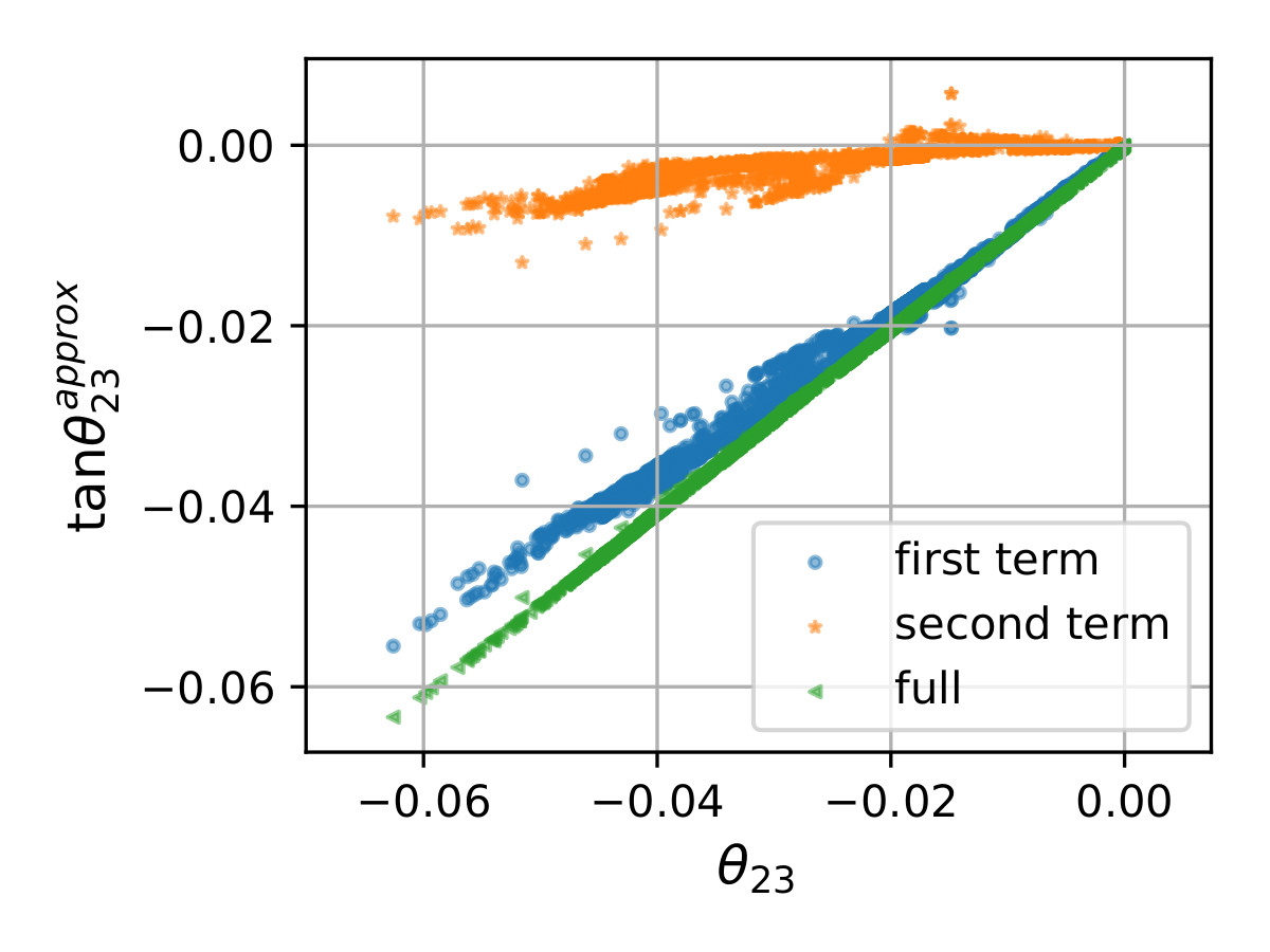
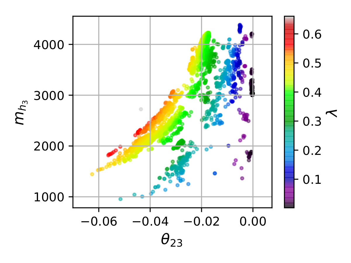
Figure 1: Left panel: $\tan\theta_{23}$ approximation showed in equation (64). Right panel: The mass of the heaviest CP-even Higgs as function of $\theta_{13}$ and $\lambda$.

Left panel of Figure 1 shows in the x-axes the value of $\theta_{23}$ computed by NMSSMtools and in the y-axes the analytical approximation described in eq. (64), as one can see in the Figure there is a good agreement between the analytical expression and the numerical value (green points), and it is clear that the main contribution to $\theta_{23}$ comes from the first term of eq. (64) (blue points). Right panel of Figure 1 shows the relation between $\theta_{23}$ and $m_{h_{3}}$ for constant values of $\lambda$. There is a trend: larger values of $|\theta_{23}|$ correspond to smaller values of $m_{h_{3}}$, except for very small values of $|\theta_{23}|$ where the two parameters seem to be uncorrelated. Still, eq. (64) shows that the value of $\tan{\theta_{23}}$ is not directly related to the scale of the heaviest Higgs, but instead it is related to the value of $\lambda$, $\mu$ and $\tan\beta$ .

Although the Higgs boson masses get important contributions from loop corrections, it is possible to get some information from the tree level expressions for $m_{h_{1}}$ and $m_{h_{2}}$. For large values of $\tan\beta$ and $M_{A}^{2}$,

$$[m_{h_{2/1}}^{2}]^{\mathrm{tree}} = \frac{1}{2}\left\{M_{Z}^{2}+\frac{1}{2}\kappa v_{s}(4\kappa v_{s}+\sqrt{2}A_{\kappa})\right.$$ (65)

$$\qquad\left.\pm\sqrt{\left[M_{Z}^{2}-\frac{1}{2}\kappa v_{s}(4\kappa v_{s}+\sqrt{2}A_{\kappa})\right]^{2}+\frac{v^{2}}{v_{s}^{2}}\left[2\lambda^{2}v_{s}^{2}-M_{A}^{2}{\sin{2\beta}}^{2}\right]^{2}}\right\}$$

where $v_{S}=\sqrt{2}\mu/\lambda$ (see Eq. (32) of [115]). In order to get a constrain for the initial parameters from the condition of small mass difference between the two lightest Higgs states, we require a small mass difference between the tree level masses showed in eq. (65). But, since the tree level expression do not precisely reproduce the masses of the Higgs states we request the mass square difference at tree level to be smaller than $M_{Z}^{2}$, meaning that both terms inside the square root should be smaller than $M_{Z}^{4}$.
Let us focus on the first term, for $A_{\kappa}\gg M_{Z}$ there should be a correlation between $A_{\kappa}$ and $\kappa v_{s}$ such that there is a cancellation that leads to an order $M_{Z}^{2}$ value. Note that the average of the tree-level squared masses also requires this cancellation to occur in order to get the masses of the Higgs states in the desired range.
For $|A_{\kappa}|\gg M_{Z}$ we expect,

$$A_{\kappa}\simeq-2\sqrt{2}\kappa v_{s}.$$ (66)

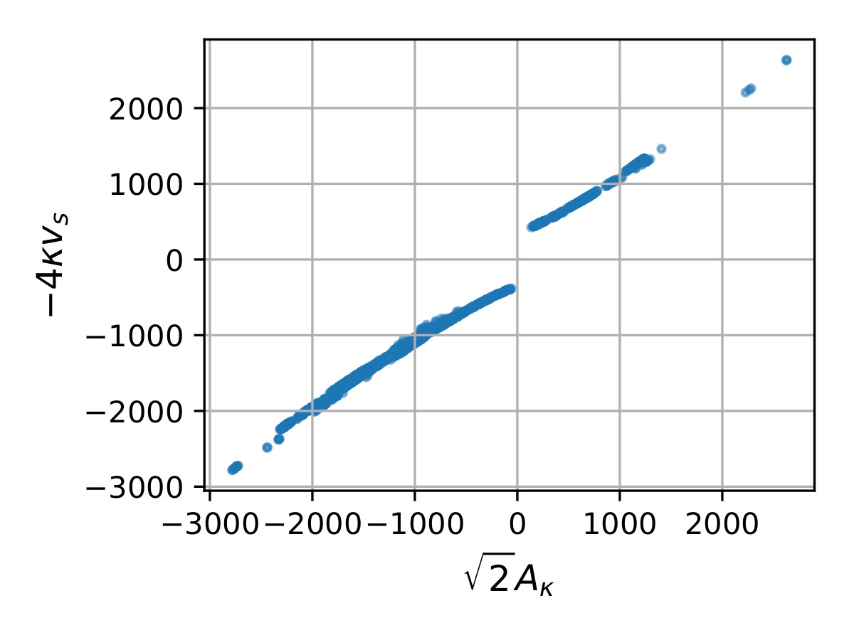
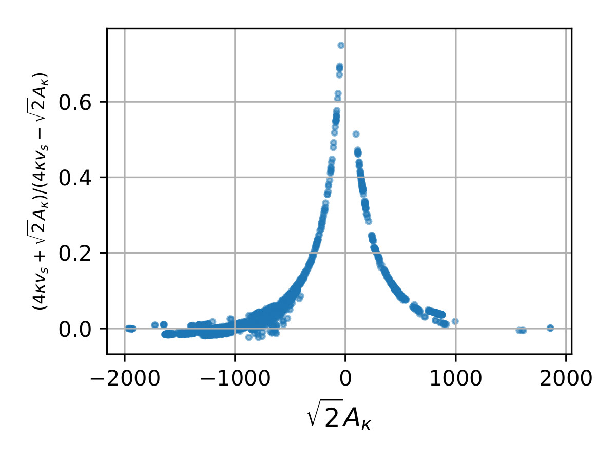
Figure 2: Left panel shows the relation between $A_{\kappa}$ and $\kappa v_{s}$. Right panel shows the relation between $A_{\kappa}$ and the degree of cancellation of $4\kappa v_{s}+\sqrt{2}A_{\kappa}$ for the sample of pNMSSM points considered.

Figure 2 shows the relation between $A_{\kappa}$ and $\kappa v_{s}$, as manifested in the figure for $|A_{\kappa}|\gtrsim 600$ GeV the approximation of eq. (66) works within an error smaller than $5\%$.

Furthermore, using eq. (66) it is possible to simplify other parameters relevant in the Higgs sector, eq. (30) of [115] gives a simplified expression for the mass of the light pseudoscalar,

$$m_{A_{1}}^{2} \simeq -\frac{3}{\sqrt{2}}\kappa v_{s}A_{\kappa}.$$ (67)

Putting eq. (66) into eq. (67) we write the mass of the lightest pseudoscalar in terms of $\kappa$ and $v_{s}$,

$$m_{A_{1}}^{2} \simeq 6\,\kappa^{2}\,v_{s}^{2}.$$ (68)

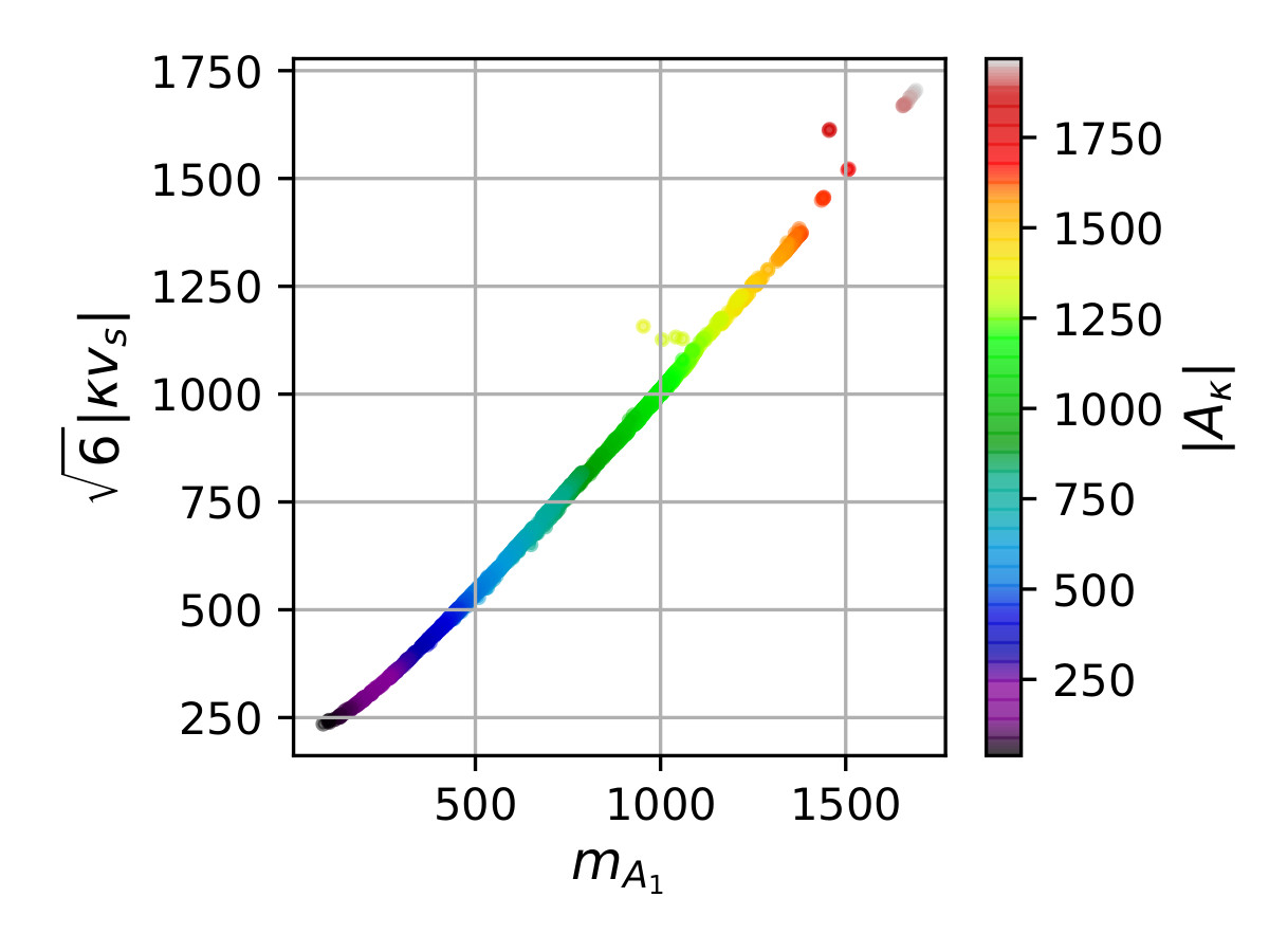
Figure 3: Comparison between the mass of the lightest pseudoscalar computed by NMSSMtools and the approximate analytical value described in eq. (68). The colour code shows the value of $A_{\kappa}$, which as described in eq. (66) it is related with the value of $\kappa v_{s}$.

Figure 3 shows the comparison between eq. (68) and the value computed by NMSSMtools. It can be seen that for $m_{A_{1}}>500$ GeV eq. (68) is a pretty good representation for the light pseudoscalar mass.

For completeness, it is worth mentioning that the second term inside the squared root of eq. (65) is suppressed by a factor $v_{s}^{\,-2}$, as such we do not expect to get any good correlation of parameters from there.

All the information, presented above, are useful for determining an optimal range of parameters in order to perform a specialised parameters scan dedicated for studying mass-degenerate Higgs region(s).

4 The two lightest CP-even Higgses at the LHC

In this section we will use the results of the scan and the analytical relations for the couplings and signal strengths to study the parameter space where the two lightest CP-even Higgs states mimic the SM-Higgs signals.

First, we have to verify the validity of the analytic expressions for the signal strengths comparing these expressions with the numerical values computed by NMSSMtools.

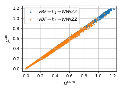
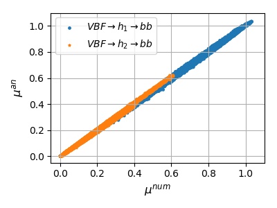
Figure 4: Shows the $\mu$ factor for VBF$\rightarrow h_{i}\rightarrow WW/ZZ$ (left panel), and VBF$\rightarrow h_{i}\rightarrow bb$ (right panel) for the pNMSSM posterior sample considered which has $m_{h_{2}}-m_{h_{1}}<3$ GeV with both $m_{h_{1}}$ and $m_{h_{2}}$ allowed within [$122$, $128$] GeV.

Figure 4 shows the comparison between the signal strengths computed by NMSSMtools, $\mu^{\mathrm{num}}$, and the analytic approximations showed in eqs. (15)-(18), $\mu^{\mathrm{an}}$, for VBF$\rightarrow h_{i}\rightarrow WW/ZZ$ (left panel) and VBF$\rightarrow h_{i}\rightarrow bb$ (right panel). From the figure we see that there is a good agreement between the analytical approximation and the numerical computation.

Now, let us identify the relevant parameters that produce deviation from experimental measurement. Writing the couplings, widths and signal strengths in terms of the mixing angles, for small values of $\theta_{12}$ and $\theta_{23}$, see eqs. (2) and (51),

$$g_{h_{i}b_{L}b_{R}^{c}}\simeq\frac{m_{b}}{\sqrt{2}v}\left\{\begin{array}[h]{cc}c_{13}+(c_{13}\theta_{12}-s_{13}\theta_{23})\tan\beta,&i=1\\ -s_{13}-(s_{13}\theta_{12}+c_{13}\theta_{23})\tan\beta,&i=2\end{array}\right.$$ (77)

$$g_{h_{i}Z_{\mu}Z_{\nu}}\simeq g_{\mu\nu}\frac{g_{1}^{2}+g_{2}^{2}}{\sqrt{2}}v\left\{\begin{array}[h]{cc}c_{13},&i=1\\ -s_{13},&i=2\end{array}\right.$$

$$g_{h_{i}W_{\mu}^{+}W_{\nu}^{-}}\simeq g_{\mu\nu}\frac{g_{2}^{2}}{\sqrt{2}}v\left\{\begin{array}[h]{cc}c_{13},&i=1\\ -s_{13},&i=2\end{array}\right..$$

Using eq. (77) and eq. (13) we get,

$$\Gamma_{1}/\Gamma_{SM} = (1-\mathrm{BR}_{bb})(c_{13})^{2}+\mathrm{BR}_{bb}[c_{13}+c_{13}\theta_{12}\tan\beta-s_{13}\theta_{23}\tan\beta]^{2}$$ (78)

$$\textrm{ and }\Gamma_{2}/\Gamma_{SM} = (1-\mathrm{BR}_{bb})(s_{13})^{2}+\mathrm{BR}_{bb}[s_{13}+s_{13}\theta_{12}\tan\beta+c_{13}\theta_{23}\tan\beta]^{2}.$$ (79)

Finally, eq. (15)-(16) can be written in terms of the mixing angles as

$$\mu_{VBF\rightarrow h_{1}\rightarrow WW/ZZ}^{\mathrm{an}} \simeq \frac{(c_{13})^{4}}{(1-\mathrm{BR}_{bb})(c_{13})^{2}+\mathrm{BR}_{bb}(c_{13}+c_{13}\theta_{12}\tan\beta-s_{13}\theta_{23}\tan\beta)^{2}},$$ (80)

$$\mu_{VBF\rightarrow h_{2}\rightarrow WW/ZZ}^{\mathrm{an}} \simeq \frac{(s_{13})^{4}}{(1-\mathrm{BR}_{bb})(s_{13})^{2}+\mathrm{BR}_{bb}(s_{13}+s_{13}\theta_{12}\tan\beta+c_{13}\theta_{23}\tan\beta)^{2}},$$ (81)

$$\mu_{VBF\rightarrow h_{1}\rightarrow bb}^{\mathrm{an}} \simeq \frac{(c_{13})^{2}(c_{13}+c_{13}\theta_{12}\tan\beta+s_{13}\theta_{23}\tan\beta)^{2}}{(1-\mathrm{BR}_{bb})(c_{13})^{2}+\mathrm{BR}_{bb}(c_{13}+c_{13}\theta_{12}\tan\beta-s_{13}\theta_{23}\tan\beta)^{2}},\textrm{ and }$$ (82)

$$\mu_{VBF\rightarrow h_{2}\rightarrow bb}^{\mathrm{an}} \simeq \frac{(s_{13})^{2}(s_{13}+s_{13}\theta_{12}\tan\beta+c_{13}\theta_{23}\tan\beta)^{2}}{(1-\mathrm{BR}_{bb})(s_{13})^{2}+\mathrm{BR}_{bb}(s_{13}+s_{13}\theta_{12}\tan\beta+c_{13}\theta_{23}\tan\beta)^{2}}.$$ (83)

From eqs.(80)-(83) we see that the signal strengths depend on four parameters: $\theta_{13}$, $\theta_{23}$, $\theta_{12}$ and $\tan\beta$. However, in the limit where $\theta_{12}\tan\beta\ll\theta_{13}$, which is the case for the pNMSSM posterior sample analysed, the number of parameters reduces to two:

$$\theta_{13}\ ,\qquad\theta_{23}\tan\beta.$$

From eqs. (80)-(83), one can see that the dependence on $\theta_{12}$ always appears as a factor in the expression $\cos{\theta_{13}}(1+\theta_{12}\tan\beta)$ or $\sin{\theta_{13}}(1+\theta_{12}\tan\beta)$. Therefore for $\theta_{12}\tan\beta\ll 1$ the contribution of $\theta_{12}$ is negligible.

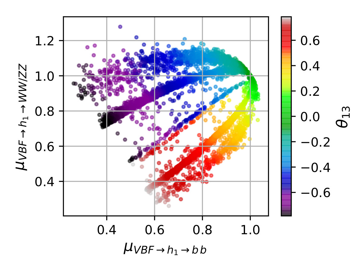
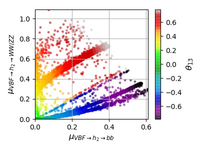
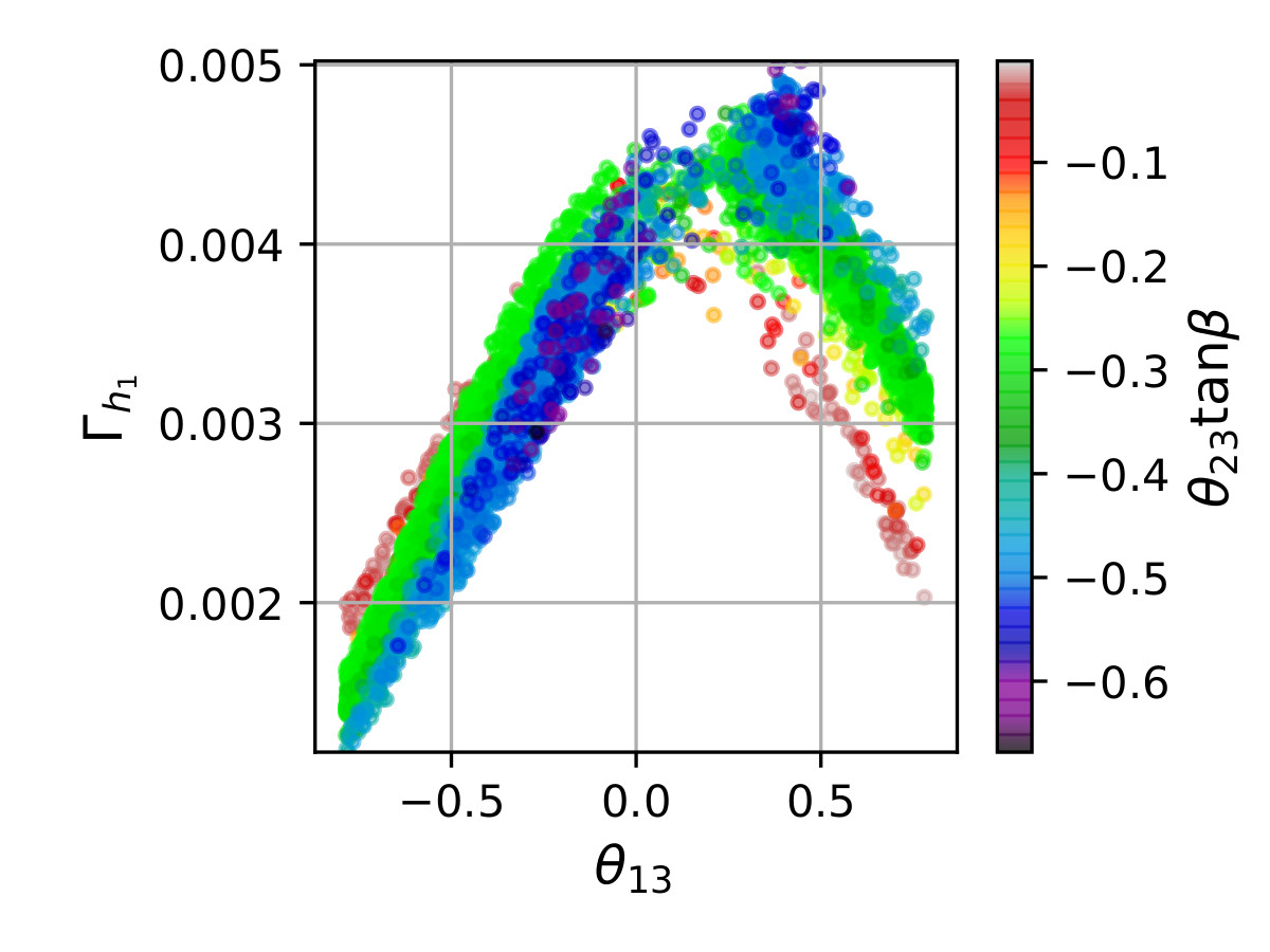
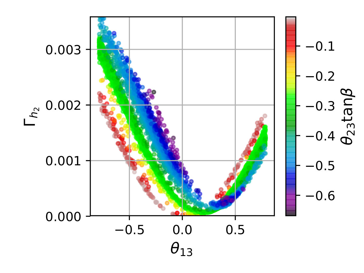
Figure 5: Top panels show the relation between both $\mu$ factors in terms of $\theta_{13}$ for $h_{1}$ (top left) and $h_{2}$(top right), the colour code shows the dependence on $\theta_{13}$. Bottom row of plots show the width of $h_{1}$ (bottom left) and $h_{2}$ (bottom right) as function of $\theta_{13}$. The colour code shows the dependence with respect to $\theta_{23}\tan\beta$.

To understand the dependence of the signal strengths with respect to $\theta_{13}$ and $\theta_{23}\tan\beta$ let us start analysing the relation between the signal strengths for a given Higgs state. The top row of Figure 5 shows the correlations between $\mu_{VBF\rightarrow h_{i}\rightarrow WW/ZZ}$ and $\mu_{VBF\rightarrow h_{i}\rightarrow bb}$ for $h_{1}$ (top left) and $h_{2}$ (top right); for $h_{1}$ we can see that the difference between the $b\bar{b}$ and $WW/ZZ$ channel signal strengths is not small. In fact, this could be taken to imply that it is not possible to reproduce the experimental results with such differences. However, looking at the right panel of the Figure and using the colour code to select regions with constant values of $\theta_{13}$, it is possible to compare the rates of the signal strengths for both Higgs bosons. The plots show that the enhancement(suppression) of one channels of $h_{1}$ is more or less compensated with a suppression(enhancement) in the same channel of $h_{2}$.

The analytic expressions for the widths of the Higgs states, eqs. (78) and (79), show that the term proportional to $\theta_{23}\tan\beta$ has a minus sign in the width of $h_{1}$ and plus sign in the width of $h_{2}$, decreasing(increasing) the decay rate of $h_{1}\rightarrow bb$ while increasing(decreasing) the decay rate of $h_{2}\rightarrow bb$ as $|\theta_{23}|$ increases its value.
The bottom row of Figure 5 shows the width of $h_{1}$ and $h_{2}$ as function of $\theta_{13}$ and $\theta_{23}\tan\beta$. The figure agrees with what we expected from the approximate expressions, eqs.(78) and (79), a function dominated by $\cos^{2}{\theta_{13}}$ for $h_{1}$ and $\sin^{2}{\theta_{13}}$ for $h_{2}$, the phase of the distributions varies with the values of $|\theta_{23}\tan\beta|$.

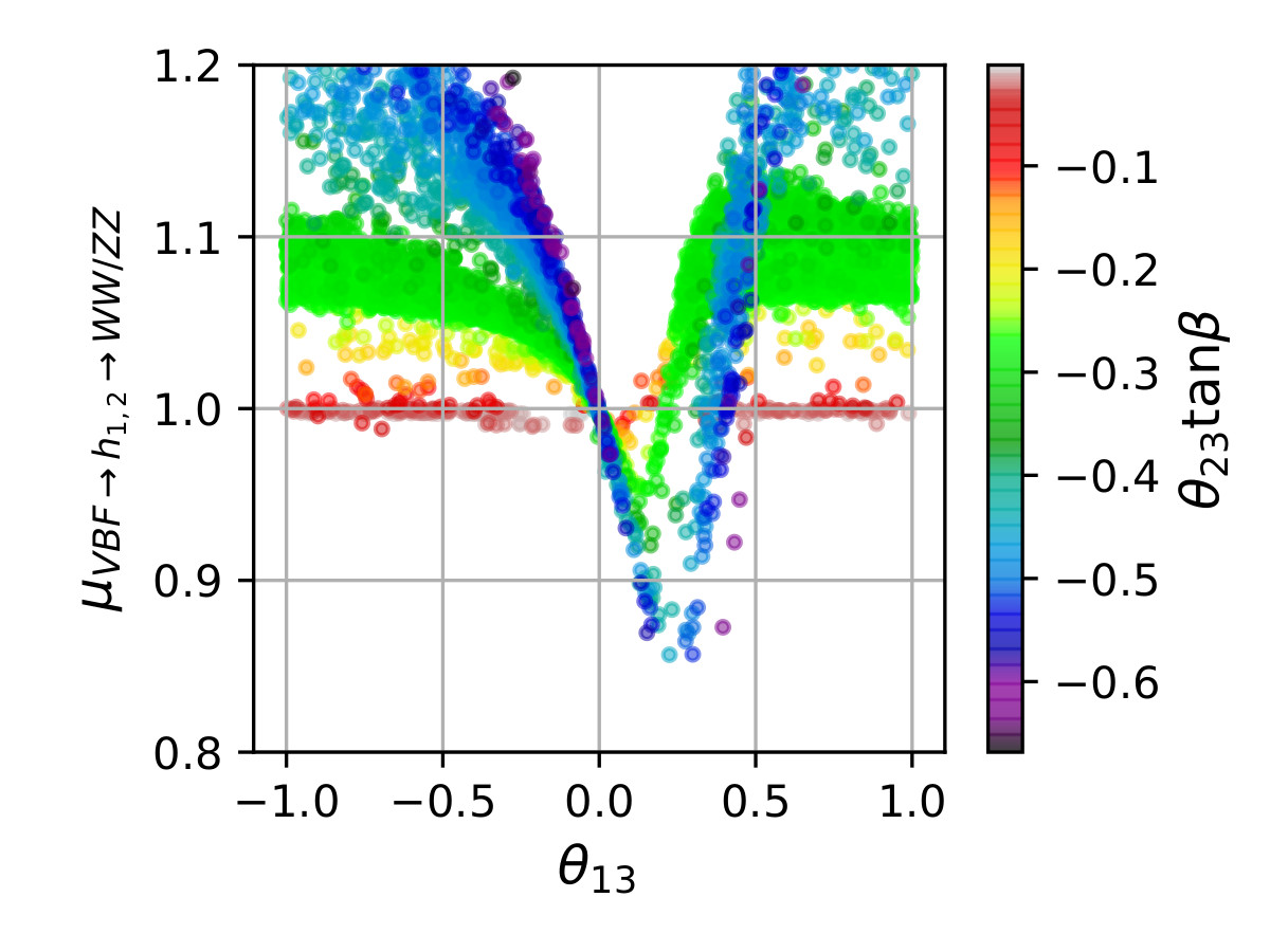
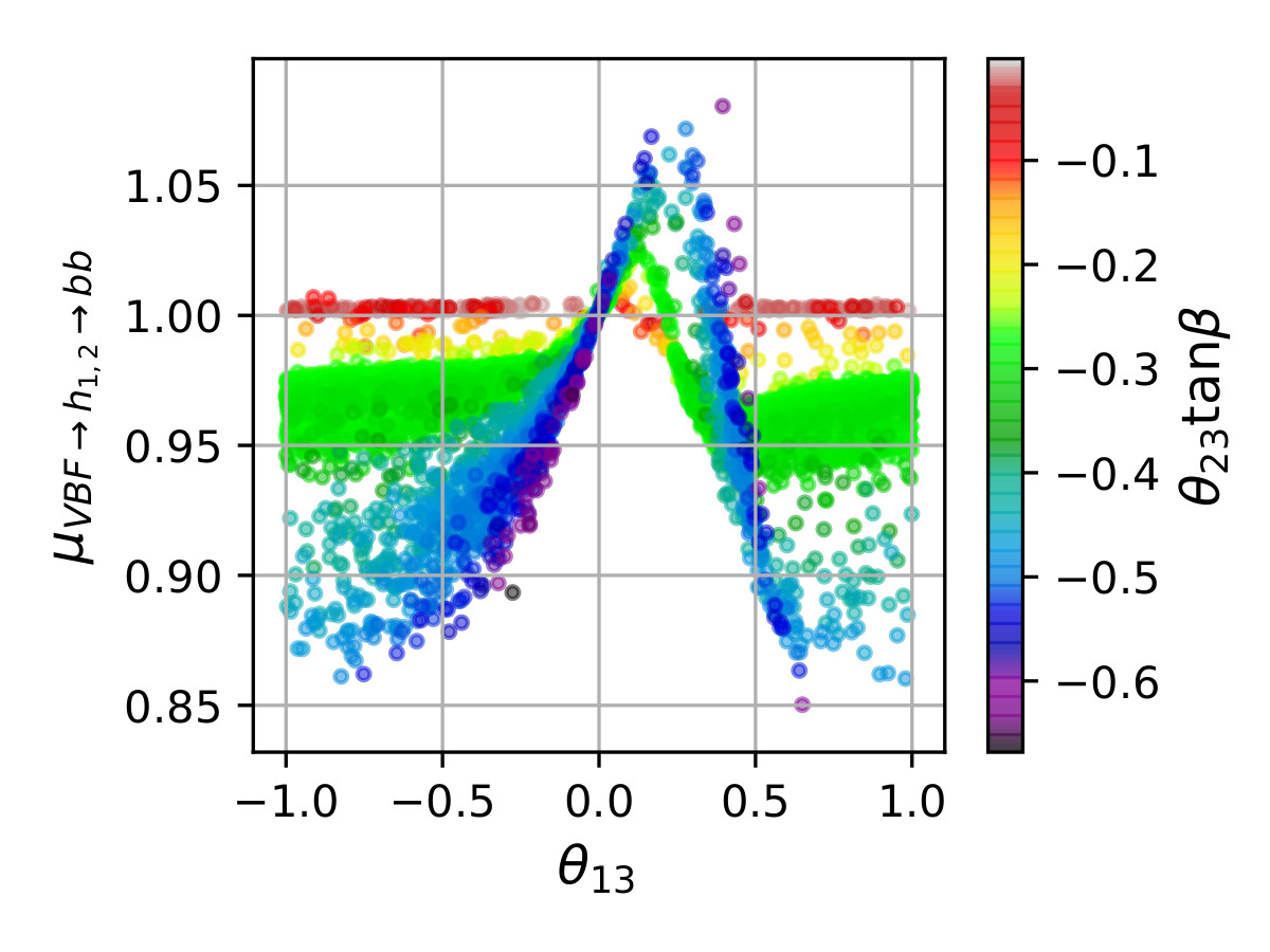
Figure 6: Shows the signal strength of the superposition of the two Higgs states for vector-boson fusion production and WW/ZZ decay (left panel), and $bb$ decay (right panel). For both plots we show the dependence of the signal strength respect to $\theta_{13}$ and $\theta_{23}\tan\beta$.

Let us analyse the global signal strengths. Figure 6 shows the sum of the signal strengths of vector-boson fusion production and decay to $WW/ZZ$ (left panel) and to $bb$ (right panel), these factors represent the global enhancement or suppression of the superposition of the two signals respect to the signal of the standard Higgs. It is important to keep in mind that to get the global signal strengths we sum the contributions of the individual signal strengths, which is allowed since we require the mass difference of the two lightest CP-even Higgs states to be small enough not to be resolved by current experiments, but much larger than the width of the particles to neglect interference effects.

There are several points we would like to comment from Figure 6, the departure of the signal strength increases with the size of $\theta_{23}\tan\beta$ as in the case of the individual signal strengths. The modification of the signal strengths for $h_{1}$ is “compensated” by the modifications of the signal strengths for $h_{2}$ and therefore the total effect is smaller than the one for the individual rates but still not negligible. Regarding the relation between the two global signals strengths it is clear from Figure 6 that $\mu_{VBF\rightarrow h_{1,2}\rightarrow WW/ZZ}$ has opposite behaviour and larger range with respect to $\mu_{VBF\rightarrow h_{1,2}bb}$.

There are two regions that seem to be in full agreement with the SM (the signal strength is $\simeq 1$): the region where $\theta_{23}\simeq 0$ and the region where $\theta_{13}\simeq 0$, as we expected. There is a third region where $\theta_{13}$ is between 0.2 and 0.4, where for a very precise value of $\theta_{23}$ the signal strength is very close to one. On the other hand, for small values of $\theta_{23}$, let’s say $\theta_{23}\tan\beta\gtrsim-0.25$, the deviation from one of the signal strength is very small, very precise measurements will be necessary to resolve it.

There is one last comment about Figures 5 and 6. We are able to fully describe the rates and the widths of $h_{1}$ and $h_{2}$ in terms of two parameters: $\theta_{13}$ and $\theta_{23}\tan\beta$, instead of three, indicating that $\theta_{12}\tan\beta\ll 1$ for the set of successful scanned points.

So far we have focused our study to two channels: VBF$\rightarrow h_{i}\rightarrow WW/ZZ$ and VBF$\rightarrow h_{i}\rightarrow bb$, but the current measurements of the Higgs couplings constrain several more channels. Let us comment about the most relevant production and decays:

1. Production processes like gluon-gluon fusion (GGF) and Higgs production associated to top quarks (ttH) are very important. To analyse these let us go back to eqs.(2), which describe the couplings of the Higgs states to top quarks,

   $$\hat{g}_{h_{i}tt}=U_{i1}-U_{i2}\cot\beta\simeq\left\{\begin{array}[h]{l r}c_{13}-(c_{13}\theta_{12}-s_{13}\theta_{23})\cot\beta,&i=1\\ -s_{13}+(s_{13}\theta_{12}+c_{13}\theta_{23})\cot\beta,&i=2\end{array}\right..$$

   Comparing $\hat{g}_{g_{i}tt}$ with $\hat{g}_{g_{i}bb}$ we see that the contribution from $\theta_{23}$ is $\cot^{2}\beta$ times smaller for $\hat{g}_{h_{i}tt}$ than for $\hat{g}_{h_{i}bb}$, therefore we expect the contribution of $\theta_{23}$ to be very tiny and the production processes of GGF and ttH to behave as vector-boson fusion for given values of $\theta_{13}$ and $\theta_{23}\tan\beta$.
   

2. The Higgs decay to photons was one of the most important channels for the discovery of a new particle, where the main contribution to the decay of the standard Higgs to photons is through a loop of W bosons. We expect that the decay of the Higgs states to photons with respect to the value of the standard Higgs scale as the decay to WW/ZZ.

3. The decay of the Higgs states to taus with respect to the value of the standard Higgs will scale as the decay of the Higgs states to bottom quarks.

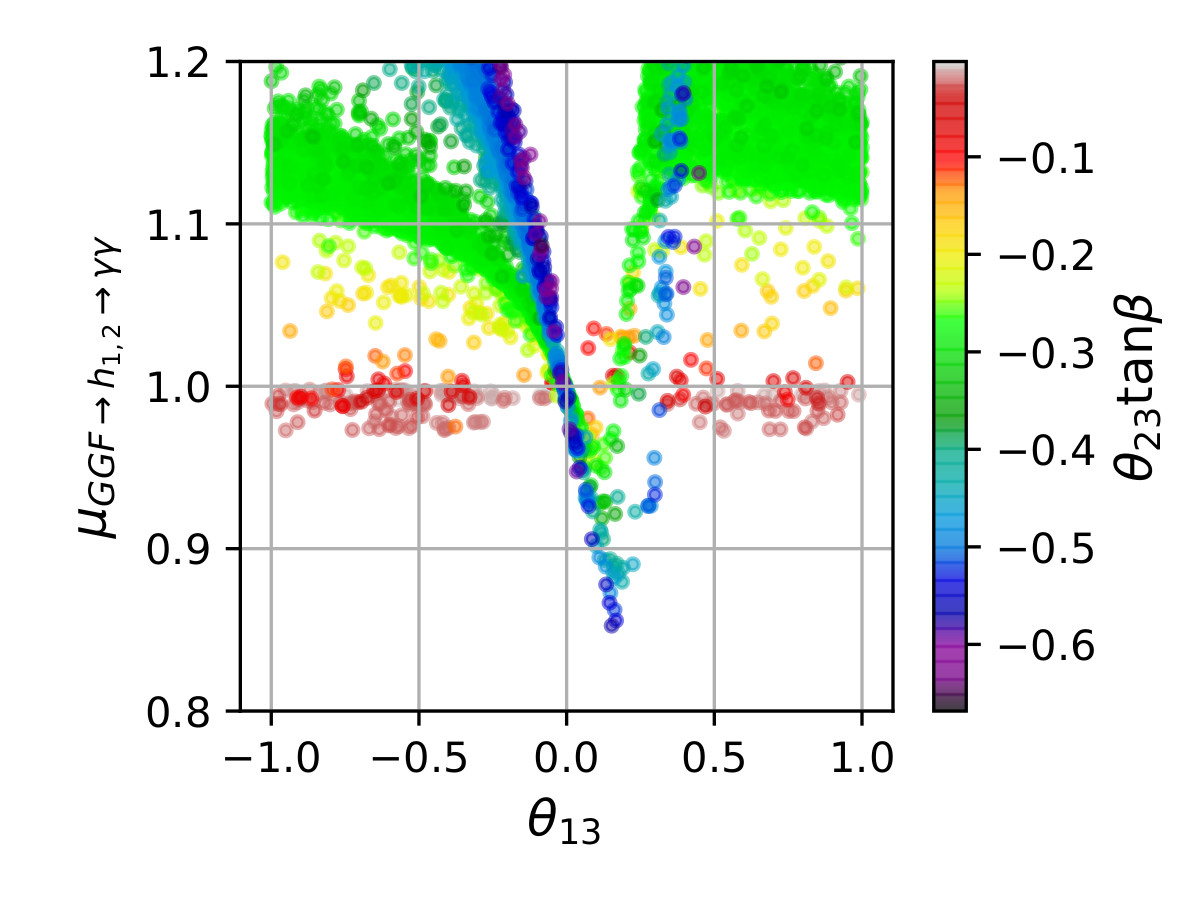
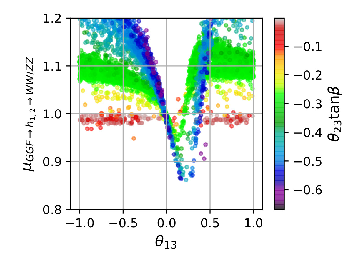
Figure 7: Signal strengths for gluon-gluon fusion production processes and $\gamma\gamma$ decay (left panel), and $WW/ZZ$ decay (right panel).

To complete the description of the signals of the two lightest CP-even Higgs states, in Figure 7 we show the signal strengths for GGF$\rightarrow h_{1,2}\rightarrow WW/ZZ$ (left panel) and GGF$\rightarrow h_{1,2}\rightarrow\gamma\gamma$ (right panel). As we expected, the gluon-gluon fusion production of the Higgses and decay to WW/ZZ is pretty similar to the vector-boson fusion production, on the other hand, the decay to photons shows a larger departure.

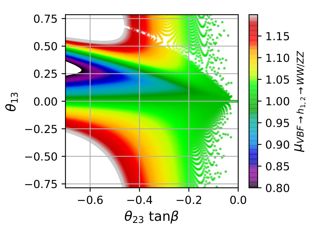
Figure 8: Left panel shows the values of $\theta_{13}$ and $\theta_{23}\tan\beta$ for the successful scanned points, the colours indicate the value of the signal strength. Right panel show the analytic solution for $\theta_{13}$ as a function of $\theta_{23}\tan\beta$ and the signal strength described in eq. (85).

So far we have seen that the leading behaviour of the signal strengths is given by $\theta_{13}$ and $\theta_{23}\tan\beta$. In the limit where $\theta_{12}\simeq 0$, we write a biunivocal function to determine one (of these parameters) in terms of the other. An approximate relation between $\theta_{13}$ and $\theta_{23}\tan\beta$ might be useful to study the region around $0.2\lesssim\theta_{13}\lesssim 0.4$ where it seems possible to mimic the signal of the standard Higgs and make it indistinguishable even for very precise experimental measurements. To determine the relation between the parameters we choose the to solve the equation:

$$\mu_{VBF\rightarrow h_{1}\rightarrow WW/ZZ}+\mu_{VBF\rightarrow h_{2}\rightarrow WW/ZZ}=1+\delta.$$ (84)

By taking $\mu_{VBF\rightarrow h_{1}\rightarrow WW/ZZ}$ and $\mu_{VBF\rightarrow h_{2}\rightarrow WW/ZZ}$ from eqs. (80) and (81), neglecting the terms proportional $\theta_{12}$, and rewriting the $\sin\theta_{13}$ and $\cos(\theta_{13})$ in terms of $\sin(2\,\theta_{13})$ and $\cos(2\,\theta_{13})$ we can simplify eq. (84) to get a quadratic equation in $\cot(2\,\theta_{13})$. So, there are two solutions for $\theta_{13}$:

$$\cot 2\theta_{13} = \frac{\mathrm{BR}_{bb}(1+\delta)\tan^{2}\beta\,\theta_{23}^{2}-\delta}{2\,\delta\,\tan\beta\,\theta_{23}}$$ (85)

$$\pm\frac{\sqrt{[\delta+\mathrm{BR}_{bb}(1+\delta)\theta_{23}^{2}\tan^{2}\beta][\mathrm{BR}_{bb}(\mathrm{BR}_{bb}-\overline{\mathrm{BR}}_{bb}\delta)\theta_{23}^{2}\tan^{2}\beta-\overline{\mathrm{BR}}_{bb}\delta]}}{2\sqrt{\mathrm{BR}_{bb}}\,\delta\,|\tan\beta\,\theta_{23}|}$$

where $\overline{\mathrm{BR}}_{bb}=1-\mathrm{BR}_{bb}$. For $\delta=0$ the solution simplifies to

$$\cot 2\theta_{13}=\frac{1+\mathrm{BR}_{bb}(-4+\theta_{23}^{2}\,\tan^{2}\beta)}{4\mathrm{BR}_{bb}\,\theta_{23}\,\tan\beta}$$ (86)

With eq. (85) we are able to determine $\theta_{13}$ in terms of $\theta_{23}\tan\beta$ and $\delta$. Figure 8 shows the comparison between the semi-analytical relation in eq. (85) and the numerical results from our scans. Although it is not a precise relation, eq. (85) gives a very good approximation to the correlation between $\theta_{13}$ and $\theta_{23}$ for a fixed value of $\delta$.

5 Searching for mass-degenerate Higgses

As commented in references [12] and [16] there are ways to test the existence of mass-degenerate states. The determinant of a signal strengths square matrix could give information about the number of resonances. If the determinant of the square matrix is equal to zero then the existence of a single Higgs resonance will be enough to reproduce the signal strengths.
For simplicity we will use a compact notation: $\mu_{ij}=\mu_{i\rightarrow j}$, where $i$ represents the production mode and $j$ the decay channel. Considering two square matrices,

$$R^{A}=\left(\begin{array}[h]{cc}\mu_{GGF,\gamma\gamma}&\mu_{GGF,\tau\tau}\\ \mu_{VBF,\gamma\gamma}&\mu_{VBF,\tau\tau}\end{array}\right),\ \ R^{B}=\left(\begin{array}[h]{cc}\mu_{GGF,\gamma\gamma}&\mu_{GGF,WW}\\ \mu_{VBF,\gamma\gamma}&\mu_{VBF,WW}\end{array}\right)$$ (91)

the condition for the determinant to be non-zero can be written in terms of the ratios

$$\frac{\mu_{VBF,WW}}{\mu_{VBF,\gamma\gamma}}\neq\frac{\mu_{GGF,WW}}{\mu_{GGF,\gamma\gamma}}\ \ \ \mathrm{and}\ \ \ \frac{\mu_{VBF,\tau\tau}}{\mu_{VBF,\gamma\gamma}}\neq\frac{\mu_{GGF,\tau\tau}}{\mu_{GGF,\gamma\gamma}}.$$ (92)

Parameter	ATLAS + CMS
$\mu_{V,\gamma\gamma}$	$1.05^{+0.44}_{-0.41}$
$\mu_{V,ZZ}$	$0.47^{+1.37}_{-0.92}$
$\mu_{V,WW}$	$1.38^{+0.41}_{-0.37}$
$\mu_{V,\tau\tau}$	$1.12^{+0.37}_{-0.35}$
$\mu_{V,bb}$	$0.65^{+0.31}_{-0.29}$
$\mu_{F,\gamma\gamma}$	$1.16^{+0.27}_{-0.24}$
$\mu_{F,ZZ}$	$1.42^{+0.37}_{-0.33}$
$\mu_{F,WW}$	$0.98^{+0.22}_{-0.20}$
$\mu_{F,\tau\tau}$	$1.06^{+0.60}_{-0.56}$
$\mu_{F,bb}$	$1.15^{+0.99}_{-0.94}$

Table 3: Ten parameter fit of $\mu_{F}^{f}$ and $\mu_{V}^{f}$. Table 15 of reference [1]

To check if it is possible to establish the existence of two resonances in the NMSSM we consider the set of pNMSSM posterior sample described in section 3 and check for points which are within one and three sigma of the particular signal strengths listed in Table 3.

Figure 9 shows the comparison between the ratios of the signal strengths in eq. (92). The upper (lower) panel shows all the points that are within three (one) sigma of the values of the individual rates. The points are ordered in such a way that smaller values of $|\theta_{23}\tan\beta|$ are on top. Notice that in the lower panel the one sigma region do not contain the point $\{1,1\}$, which is what we expect from a standard Higgs, this is because the experimental value of $\mu_{VBF,bb}$ is $0.65^{+0.31}_{-0.29}$ (see Table 3), it doesn’t include the SM value at one sigma. The left panel of Figure 9 shows that the ratios between $WW$ and $\gamma\gamma$ signal strength are basically the same, meaning that the determinant of $R_{A}$ is approximately zero and therefore in agreement with a single resonance hypothesis. On the other hand the ratios between $\tau\tau$ and $\gamma\gamma$ signal strength are slightly separated from the dotted line, the determinant of $R_{B}$ is different from zero. In general we would expect that if there is more than one Higgs state the ratio between two signal strengths with the same production process and different decay product is not going to be equal to one. However, we get that this ratio is almost the same for the rate between gluon-gluon fusion and for vector-boson fusion production processes, which indicates that both production cross-sections are very similar for a given Higgs state. Therefore, it doesn’t seem possible to distinguish between single and double resonances from those measurements for this set of scanned points.

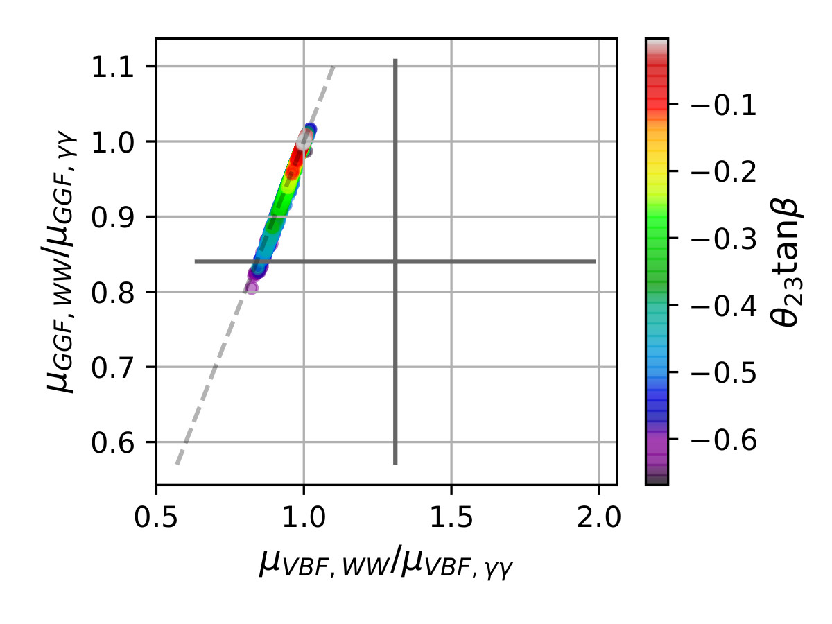
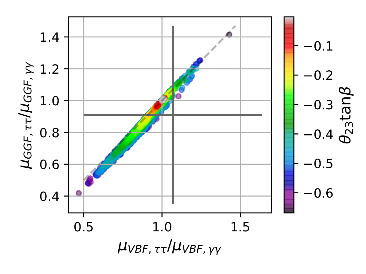
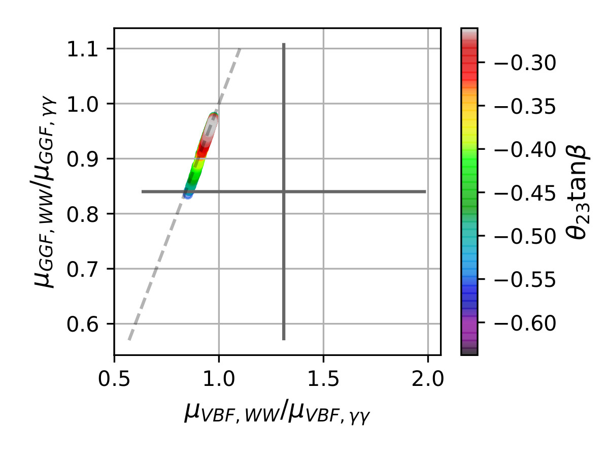
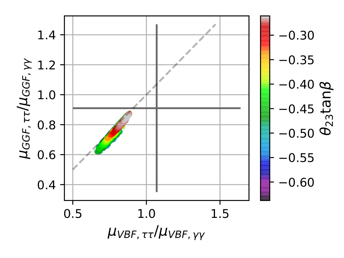
Figure 9: Comparison between ratios of the signal strengths from the pNMSSM sample considered. The Upper (lower) row shows points with individual signal strength within three (one) sigma with respect to the experimental values. The large dark gray lines represent the error bars of the experimental value for each of the rates. The dotted line indicates det($R$)=0.

Is there any observable that could be used to distinguish between single and double resonance signals? From the discussion of the previous sections we have learned that $\mu_{VBF,bb}$ have an opposite behaviour with respect to the other signal strength we have considered, therefore we may suspect that the production of Higgs states associated to bottom quarks compared to the production associated to vector bosons would give a larger departure from the SM signal than the comparison between vector-boson fusion and gluon-gluon fusion.
Let us consider the matrices,

$$R^{C}=\left(\begin{array}[h]{cc}\mu_{BBF,\gamma\gamma}&\mu_{BBF,\tau\tau}\\ \mu_{VBF,\gamma\gamma}&\mu_{VBF,\tau\tau}\end{array}\right),\ \ R^{D}=\left(\begin{array}[h]{cc}\mu_{BBF,\gamma\gamma}&\mu_{BBF,WW}\\ \mu_{VBF,\gamma\gamma}&\mu_{VBF,WW}\end{array}\right)$$ (97)

where BBF represents the Higgs productions associated to bottom quarks. To obtain a determinant different from zero requires that ratios of the signal strengths follow:

$$\frac{\mu_{VBF,WW}}{\mu_{VBF,\gamma\gamma}}\neq\frac{\mu_{BBH,WW}}{\mu_{BBH,\gamma\gamma}}\ \ \ \mathrm{and}\ \ \ \frac{\mu_{VBF,\tau\tau}}{\mu_{VBF,\gamma\gamma}}\neq\frac{\mu_{BBH,\tau\tau}}{\mu_{BBH,\gamma\gamma}}$$ (98)

To compute the signal strength of Higgs production associated to bottom quarks we use the reduced couplings to bottom quarks computed by NMSSMtools.

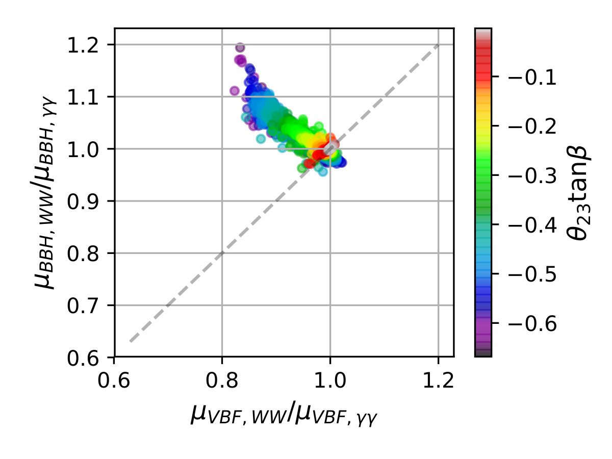
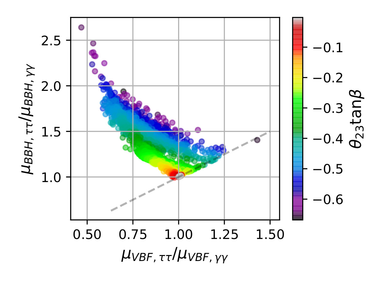
Figure 10: Comparison between vector-boson fusion and Higgs production associated to bottom quarks. Points are within three sigma of the measured individual signal strengths. The dotted line indicates det($R$)=0.

Figure 10 shows the comparison of the ratios described in eq. (10) for points that fulfill the experimental signal strength listed in Table 3 within three sigma. The figure shows that the determinant of the $R^{C}$ and $R^{D}$ is different from zero for a large part of the points, and therefore it gives a clear signature for the existence of more than one Higgs resonance.

It may be surprising to see such a large deviation from zero in the determinant of $R^{C}$ and $R^{D}$ and not in the determinant of $R^{A}$ and $R^{B}$, the main reason lies in the difference between the production processes. Although it does not seem straight forward from the analytic expressions of the full signal strength to single out this differences and directly relate them with the value of the determinants, one can always compare the production cross-sections for each Higgs state separately. If they are approximately the same, then the ratios shown in Figures 9 and 10 will be the same – and the determinant of the matrix $R$ will be approximately equal to zero.

For simplicity let us consider that the gluon-gluon fusion cross section is dominated by the coupling of the Higgs to top quarks, this consideration will allow us to have more insights of the source of discrepancy between the determinants. Eqs.(2) show that $\hat{g}_{tth_{i}}$ has an extra factor $-U_{i2}/\tan\beta$ with respect to the coupling to vector bosons, using the approximation of small $\theta_{23}$ and negligible $\theta_{12}$, the extra factor simplify to $\theta_{23}/\tan\beta$ times $\cos\theta_{13}$($\sin\theta_{13}$) for $h_{1}$($h_{2}$), a factor suppressed by $\tan\beta$. Therefore, unless $\tan\beta$ is close to one, or $\theta_{23}$ is large, we would expect very similar signal strengths for gluon-gluon fusion and vector-boson fusion for each Higgs state, in consequence the total signal strengths for the same final state will be also very similar, and the determinant of $R^{A}$ and $R^{B}$ will be close to zero.

On the contrary, if instead of gluon-gluon fusion production process we consider Higgs production associated to bottom quarks, eqs. (2) show that $\hat{g}_{bbh_{i}}$ has an extra factor $U_{i2}\tan\beta$ with respect to vector boson coupling, the factor is $\tan^{2}\beta$ larger than in the case of $\hat{g}_{tth_{i}}$. For non-negligible values of $\theta_{23}$ there will be a significant departure of signal strength of the Higgs production associated to bottom quarks with respect to the vector-boson fusion for the same final state. When computing the ratio of the total signal strength for different final states we would expect a larger deviation, in consequence the determinant of $R^{C}$ and $R^{D}$ will be different from zero.

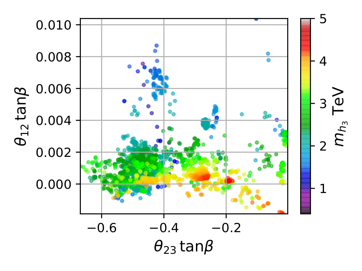
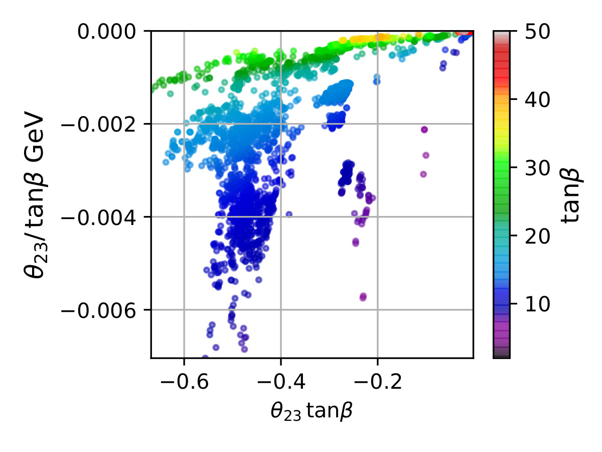
Figure 11: Left panel shows the values of $\theta_{12}$, $\theta_{23}$ and the mass of the heaviest CP-even Higgs in the colour bar. Right panel illustrate the $\theta_{23}$ dependence in the coupling of the Higgs for up-type quarks ($\theta_{23}/\tan\beta$) and down-type quarks and leptons ($\theta_{23}\tan\beta$).

These arguments describe very well a set of points with medium to large values of $\tan\beta$. For small values of $\tan\beta$ and large enough values of $\theta_{23}$ the determinant of $R^{A}$ and $R^{B}$ will also show a departure from unity. Figure 11 shows the values of $\theta_{12}$, $\theta_{23}$, $\tan\beta$ and $m_{h_{3}}$ for the pNMSSM posterior sample with $m_{h_{3}}$ larger that 1 TeV and values of $\tan\beta$ larger than 10. As we expected the value of $\theta_{23}/\tan\beta$ is tiny, which explains why the determinant of $R^{A}$ and $R^{B}$ is very close to zero. The large values of $\tan\beta$ also explain the large departure from one for the determinant of $R^{C}$ and $R^{D}$.

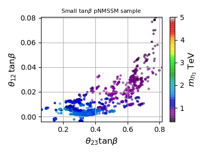
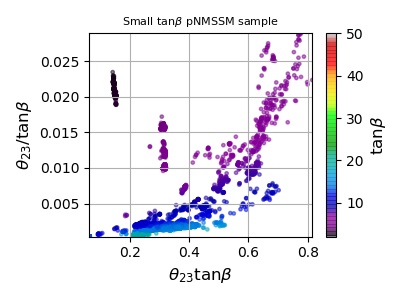
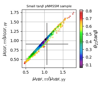
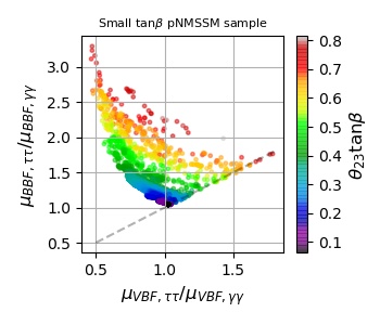
Figure 12: Top row shows the values of $\theta_{12}$ and $\theta_{23}$ with respect to $\tan\beta$ and $m_{h_{3}}$. Bottom panel show the comparison between the signal strengths of vector-boson fusion and gluon-gluon fusion (left), vector-boson fusion and Higgs production associated to bottom quarks (right), for $\tau\tau$ and $\gamma\gamma$ final states.

Our scan focused on the region of the parameter space with medium to large values of $\tan\beta$, to complete our analysis we analyse a new set of points with smaller values of $\tan\beta$ relative to the first sample set. We perform another small scan giving more preference to the region of small $\tan\beta$ and small $m_{h_{3}}$, covering $\tan\beta$ in the range of $[2.5,21]$ and $m_{h_{3}}$ in the range of [435 GeV to 2 TeV], the results are summarized in figure 12. The top row of the figure shows the values of $\theta_{12}$ and $\theta_{23}$ with respect to $m_{h_{3}}$ and $\tan\beta$. To analyse these two plots in comparison with Figure 11 we have used the same range for the variables plotted in the colour bar to make easier the comparison. First let us focus on the top-left plot of Figure 12. Note that the range of values for $|\theta_{23}\tan\beta|$ is almost the same for both samples suggesting that this parameter is directly constrained by the experimental measurements of the Higgs couplings. Smaller values of $m_{h_{3}}$ are correlated with larger values of $\theta_{12}$, still $|\theta_{23}|$ is one order of magnitude larger than $|\theta_{12}|$, meaning that the approximation of $\theta_{12}\sim 0$ is still valid. The top-right plot of Figures 11 and 12 compare the values of $\theta_{23}\tan\beta$ with $\theta_{23}/\tan\beta$ that illustrate the contribution of $\theta_{23}$ to the Higgs production associated to bottom quarks (x-axis) and gluon-gluon fusion production (y-axis).

The bottom row of Figure 12 show the values of $R^{B}$ and $R^{D}$ for the new set of scanned points. Here, points with $\theta_{23}\tan\beta\sim 0.7$ correspond to $|\theta_{23}/\tan\beta|$ up to 0.030, which is around fifty times larger than our first scan. This increment will be reflected in the value of $R^{B}$, which involves the rate plotted in the left panel of the figure. Previous studies, like [12, 13, 14] pointed out that the determinant of $R^{A}$ and $R^{B}$ will be useful to determine the existence of more than one resonance. Our analyses indicate that this is indeed the case but mostly for pNMSSM regions with relatively smaller $\tan\beta$ values and lighter $h_{3}$. The botton-right plot of Figure 12 shows the relevant ratios to compute the determinant of $R^{D}$. There is a discrepancy in the region with $|\theta_{23}\tan\beta|$ larger than $\sim 0.65$. According to the top-row plots of Figure 12, points with $|\theta_{23}\tan\beta|>0.7$ correspond to $m_{h_{3}}$ smaller that 1 TeV and $\tan\beta$ smaller than 10. Getting relatively larger values for $|\theta_{23}\tan\beta|$ in the new set of points scanned compared to the first pNMSSM posterior sample is in accord with the fact that $|\theta_{23}|$ increases as $m_{h_{3}}$ decreases for a fixed value of $\lambda$ (as discussed in section 3.3). So in the new scan by exploring $m_{h_{3}}<$ 1 TeV, we expand the range of exploration for $|\theta_{23}\tan\beta|$.

6 Conclusions

We studied the phenomenology of the two mass degenerate CP-even Higgs bosons in the NMSSM using a sample set from the parameter scan of the pNMSSM. In this scenario it is possible to reproduce the experimental signal measured by ATLAS and CMS. We parameterised the Higgs boson signal strengths using three angles and found that it is possible to write approximate expressions in terms of two parameters $\theta_{23}\tan\beta$ and $\theta_{13}$, where $\theta_{23}$ is the mixing between the singlet and the heaviest neutral Higgs of the Higgs doublet $H_{0}$ and $\theta_{13}$ the mixing between the lightest neutral scalar of the Higgs doublet and the singlet. We have focused our analysis into observables that could help to determine the existence of more that one Higgs state, leading to the following conclusions.

• To obtain two mass degenerate CP-even Higgs bosons there is required tuning associated to large values of $A_{\kappa}$, $\lambda$, $\kappa$ and $\mu$. An approximate relation between those parameters could be obtained from the tree level mass relations, although this relation simplifies the expression for the mass of the lightest pseudoscalar it does not point out to specific mass relations.

• An approximate expression for $\theta_{23}$ can be written in terms of $\mu/\lambda$ and $\tan\beta$. The allowed range for $|\theta_{23}\tan\beta|$ is between 0.0 and 0.7. Greater values can be obtained if $m_{h_{s}}\lesssim 1$ TeV and $\tan\beta\lesssim 8$ are imposed. There are no direct constraints on the mass spectra from specific values of $\theta_{23}$ but it is possible to reproduce various values of $m_{h_{3}}$ for a fixed value of $\theta_{23}$ and different values of $\lambda$.

• Analysing the Higgs bosons couplings to fermions and vector bosons, and the signal strengths, we found that the signal of the superposition of the Higgs bosons decaying to leptons (and bottom quarks) depart from the SM signal in an opposite direction with respect to vector boson final states. This is proportional to $|\theta_{23}\tan\beta|$.

• With respect to expectations due to previous studies, it was surprising to find that for medium to large values of $\tan\beta$, it is rather difficult to distinguish the two degenerate Higgs from the single Higgs scenario when the matrix of signal strengths are for vector-boson and gluon-gluon fusion Higgs productions (with the Higgs decaying to vector boson).

• By including Higgs production in association with bottom quarks in the signal strengths square matrix we found that the matrix determinant departs significantly large from the single resonance value.Therefore the process $pp\rightarrow bbh$ can be an important channel in searches for multiple Higgs states degenerate around $125\>\text{GeV}$.

References

- [1] G. Aad et al., “Measurements of the Higgs boson production and decay rates and constraints on its couplings from a combined ATLAS and CMS analysis of the LHC pp collision data at and 8 TeV,” JHEP, vol. 08, p. 045, 2016, 1606.02266.
- [2] G. Aad et al., “Measurements of the Higgs boson production and decay rates and coupling strengths using pp collision data at and 8 TeV in the ATLAS experiment,” Eur. Phys. J., vol. C76, no. 1, p. 6, 2016, 1507.04548.
- [3] M. E. Cabrera, J. A. Casas, and R. Ruiz de Austri, “Bayesian approach and Naturalness in MSSM analyses for the LHC,” JHEP, vol. 03, p. 075, 2009, 0812.0536.
- [4] M. E. Cabrera, J. A. Casas, and R. Ruiz de Austri, “MSSM Forecast for the LHC,” JHEP, vol. 05, p. 043, 2010, 0911.4686.
- [5] S. S. AbdusSalam, B. C. Allanach, F. Quevedo, F. Feroz, and M. Hobson, “Fitting the Phenomenological MSSM,” Phys. Rev., vol. D81, p. 095012, 2010, 0904.2548.
- [6] J. Alwall, P. Schuster, and N. Toro, “Simplified Models for a First Characterization of New Physics at the LHC,” Phys. Rev., vol. D79, p. 075020, 2009, 0810.3921.
- [7] D. Alves, “Simplified Models for LHC New Physics Searches,” J. Phys., vol. G39, p. 105005, 2012, 1105.2838.
- [8] A. Djouadi et al., “The Minimal supersymmetric standard model: Group summary report,” in GDR (Groupement De Recherche) - Supersymetrie Montpellier, France, April 15-17, 1998, 1998, hep-ph/9901246.
- [9] S. S. AbdusSalam, “The Full 24-Parameter MSSM Exploration,” AIP Conf. Proc., vol. 1078, pp. 297–299, 2009, 0809.0284.
- [10] C. F. Berger, J. S. Gainer, J. L. Hewett, and T. G. Rizzo, “Supersymmetry Without Prejudice,” JHEP, vol. 02, p. 023, 2009, 0812.0980.
- [11] S. S. AbdusSalam, “LHC-7 supersymmetry search interpretation within the phenomenological MSSM,” Phys. Rev., vol. D87, no. 11, p. 115012, 2013, 1211.0999.
- [12] J. F. Gunion, Y. Jiang, and S. Kraml, “Diagnosing Degenerate Higgs Bosons at 125 GeV,” Phys. Rev. Lett., vol. 110, no. 5, p. 051801, 2013, 1208.1817.
- [13] S. Munir, L. Roszkowski, and S. Trojanowski, “Simultaneous enhancement in and rates in the NMSSM with nearly degenerate scalar and pseudoscalar Higgs bosons,” Phys. Rev., vol. D88, no. 5, p. 055017, 2013, 1305.0591.
- [14] S. Moretti and S. Munir, “Two Higgs Bosons near 125 GeV in the Complex NMSSM and the LHC Run I Data,” Adv. High Energy Phys., vol. 2015, p. 509847, 2015, 1505.00545.
- [15] B. Das, S. Moretti, S. Munir, and P. Poulose, “Two Higgs bosons near 125 GeV in the NMSSM: beyond the narrow width approximation,” Eur. Phys. J., vol. C77, no. 8, p. 544, 2017, 1704.02941.
- [16] Y. Grossman, Z. Surujon, and J. Zupan, “How to test for mass degenerate Higgs resonances,” JHEP, vol. 03, p. 176, 2013, 1301.0328.
- [17] A. David, J. Heikkilä, and G. Petrucciani, “Searching for degenerate Higgs bosons,” Eur. Phys. J., vol. C75, no. 2, p. 49, 2015, 1409.6132.
- [18] M. Carena, H. E. Haber, I. Low, N. R. Shah, and C. E. M. Wagner, “Alignment limit of the NMSSM Higgs sector,” Phys. Rev., vol. D93, no. 3, p. 035013, 2016, 1510.09137.
- [19] S. F. King, M. Mühlleitner, R. Nevzorov, and K. Walz, “Natural NMSSM Higgs Bosons,” Nucl. Phys., vol. B870, pp. 323–352, 2013, 1211.5074.
- [20] U. Ellwanger, “A Higgs boson near 125 GeV with enhanced di-photon signal in the NMSSM,” JHEP, vol. 03, p. 044, 2012, 1112.3548.
- [21] J. F. Gunion, Y. Jiang, and S. Kraml, “Could two NMSSM Higgs bosons be present near 125 GeV?,” Phys. Rev., vol. D86, p. 071702, 2012, 1207.1545.
- [22] T. Gherghetta, B. von Harling, A. D. Medina, and M. A. Schmidt, “The Scale-Invariant NMSSM and the 126 GeV Higgs Boson,” JHEP, vol. 02, p. 032, 2013, 1212.5243.
- [23] S. S. AbdusSalam, “Testing Higgs boson scenarios in the phenomenological NMSSM,” 2017, 1710.10785.
- [24] U. Ellwanger and C. Hugonie, “NMSPEC: A Fortran code for the sparticle and Higgs masses in the NMSSM with GUT scale boundary conditions,” Comput. Phys. Commun., vol. 177, pp. 399–407, 2007, hep-ph/0612134.
- [25] U. Ellwanger and C. Hugonie, “NMHDECAY 2.0: An Updated program for sparticle masses, Higgs masses, couplings and decay widths in the NMSSM,” Comput. Phys. Commun., vol. 175, pp. 290–303, 2006, hep-ph/0508022.
- [26] A. Djouadi, J. Kalinowski, and M. Spira, “HDECAY: A Program for Higgs boson decays in the standard model and its supersymmetric extension,” Comput. Phys. Commun., vol. 108, pp. 56–74, 1998, hep-ph/9704448.
- [27] G. Degrassi and P. Slavich, “On the radiative corrections to the neutral Higgs boson masses in the NMSSM,” Nucl. Phys., vol. B825, pp. 119–150, 2010, 0907.4682.
- [28] F. Domingo and U. Ellwanger, “Updated Constraints from Physics on the MSSM and the NMSSM,” JHEP, vol. 12, p. 090, 2007, 0710.3714.
- [29] F. Domingo, “Update of the flavour-physics constraints in the NMSSM,” Eur. Phys. J., vol. C76, no. 8, p. 452, 2016, 1512.02091.
- [30] J. Bernon and B. Dumont, “Lilith: a tool for constraining new physics from Higgs measurements,” Eur. Phys. J., vol. C75, no. 9, p. 440, 2015, 1502.04138.
- [31] E. Boos, V. Bunichev, M. Dubinin, L. Dudko, V. Ilyin, A. Kryukov, V. Edneral, V. Savrin, A. Semenov, and A. Sherstnev, “CompHEP 4.4: Automatic computations from Lagrangians to events,” Nucl. Instrum. Meth., vol. A534, pp. 250–259, 2004, hep-ph/0403113.
- [32] A. Semenov, “LanHEP: A Package for the automatic generation of Feynman rules in field theory. Version 3.0,” Comput. Phys. Commun., vol. 180, pp. 431–454, 2009, 0805.0555.
- [33] G. Belanger, N. D. Christensen, A. Pukhov, and A. Semenov, “SLHAplus: a library for implementing extensions of the standard model,” Comput. Phys. Commun., vol. 182, pp. 763–774, 2011, 1008.0181.
- [34] A. Pukhov, E. Boos, M. Dubinin, V. Edneral, V. Ilyin, D. Kovalenko, A. Kryukov, V. Savrin, S. Shichanin, and A. Semenov, “CompHEP: A Package for evaluation of Feynman diagrams and integration over multiparticle phase space,” 1999, hep-ph/9908288.
- [35] A. Belyaev, N. D. Christensen, and A. Pukhov, “CalcHEP 3.4 for collider physics within and beyond the Standard Model,” Comput. Phys. Commun., vol. 184, pp. 1729–1769, 2013, 1207.6082.
- [36] G. Belanger, F. Boudjema, A. Pukhov, and A. Semenov, “micrOMEGAs_3: A program for calculating dark matter observables,” Comput. Phys. Commun., vol. 185, pp. 960–985, 2014, 1305.0237.
- [37] G. Belanger, F. Boudjema, A. Pukhov, and A. Semenov, “micrOMEGAs: A Tool for dark matter studies,” Nuovo Cim., vol. C033N2, pp. 111–116, 2010, 1005.4133.
- [38] G. Belanger, F. Boudjema, A. Pukhov, and A. Semenov, “Dark matter direct detection rate in a generic model with micrOMEGAs 2.2,” Comput. Phys. Commun., vol. 180, pp. 747–767, 2009, 0803.2360.
- [39] G. Belanger, F. Boudjema, A. Pukhov, and A. Semenov, “MicrOMEGAs 2.0: A Program to calculate the relic density of dark matter in a generic model,” Comput. Phys. Commun., vol. 176, pp. 367–382, 2007, hep-ph/0607059.
- [40] D. Barducci, G. Belanger, J. Bernon, F. Boudjema, J. Da Silva, S. Kraml, U. Laa, and A. Pukhov, “Collider limits on new physics within micrOMEGAs_4.3,” Comput. Phys. Commun., vol. 222, pp. 327–338, 2018, 1606.03834.
- [41] F. Ambrogi, S. Kraml, S. Kulkarni, U. Laa, A. Lessa, V. Magerl, J. Sonneveld, M. Traub, and W. Waltenberger, “SModelS v1.1 user manual: Improving simplified model constraints with efficiency maps,” Comput. Phys. Commun., vol. 227, pp. 72–98, 2018, 1701.06586.
- [42] S. Kraml, S. Kulkarni, U. Laa, A. Lessa, W. Magerl, D. Proschofsky-Spindler, and W. Waltenberger, “SModelS: a tool for interpreting simplified-model results from the LHC and its application to supersymmetry,” Eur. Phys. J., vol. C74, p. 2868, 2014, 1312.4175.
- [43] A. Buckley, “PySLHA: a Pythonic interface to SUSY Les Houches Accord data,” Eur. Phys. J., vol. C75, no. 10, p. 467, 2015, 1305.4194.
- [44] T. Sjostrand, S. Mrenna, and P. Z. Skands, “PYTHIA 6.4 Physics and Manual,” JHEP, vol. 05, p. 026, 2006, hep-ph/0603175.
- [45] W. Beenakker, R. Hopker, M. Spira, and P. M. Zerwas, “Squark and gluino production at hadron colliders,” Nucl. Phys., vol. B492, pp. 51–103, 1997, hep-ph/9610490.
- [46] W. Beenakker, M. Kramer, T. Plehn, M. Spira, and P. M. Zerwas, “Stop production at hadron colliders,” Nucl. Phys., vol. B515, pp. 3–14, 1998, hep-ph/9710451.
- [47] A. Kulesza and L. Motyka, “Threshold resummation for squark-antisquark and gluino-pair production at the LHC,” Phys. Rev. Lett., vol. 102, p. 111802, 2009, 0807.2405.
- [48] A. Kulesza and L. Motyka, “Soft gluon resummation for the production of gluino-gluino and squark-antisquark pairs at the LHC,” Phys. Rev., vol. D80, p. 095004, 2009, 0905.4749.
- [49] W. Beenakker, S. Brensing, M. Kramer, A. Kulesza, E. Laenen, and I. Niessen, “Soft-gluon resummation for squark and gluino hadroproduction,” JHEP, vol. 12, p. 041, 2009, 0909.4418.
- [50] W. Beenakker, S. Brensing, M. Kramer, A. Kulesza, E. Laenen, and I. Niessen, “Supersymmetric top and bottom squark production at hadron colliders,” JHEP, vol. 08, p. 098, 2010, 1006.4771.
- [51] W. Beenakker, S. Brensing, M. n. Kramer, A. Kulesza, E. Laenen, L. Motyka, and I. Niessen, “Squark and Gluino Hadroproduction,” Int. J. Mod. Phys., vol. A26, pp. 2637–2664, 2011, 1105.1110.
- [52] “Search for direct production of the top squark in the all-hadronic ttbar + etmiss final state in 21 fb-1 of p-pcollisions at sqrt(s)=8 TeV with the ATLAS detector,” 2013.
- [53] T. A. collaboration, “Search for squarks and gluinos with the ATLAS detector in final states with jets and missing transverse momentum and 20.3 fb-1 of TeV proton-proton collision data,” 2013.
- [54] T. A. collaboration, “Search for direct third generation squark pair production in final states with missing transverse momentum and two -jets in = 8 TeV collisions with the ATLAS detector.,” 2013.
- [55] T. A. collaboration, “Search for strong production of supersymmetric particles in final states with missing transverse momentum and at least three b-jets using 20.1 of pp collisions at = 8 TeV with the ATLAS Detector.,” 2013.
- [56] C. Collaboration, “Search for direct production of bottom squark pairs,” 2014.
- [57] C. Collaboration, “A Search for Scalar Top Quark Production and Decay to All Hadronic Final States in pp Collisions at = 8 TeV,” 2015.
- [58] S. Chatrchyan et al., “Search for supersymmetry in hadronic final states with missing transverse energy using the variables and b-quark multiplicity in pp collisions at TeV,” Eur. Phys. J., vol. C73, no. 9, p. 2568, 2013, 1303.2985.
- [59] V. Khachatryan et al., “Searches for electroweak production of charginos, neutralinos, and sleptons decaying to leptons and W, Z, and Higgs bosons in pp collisions at 8 TeV,” Eur. Phys. J., vol. C74, no. 9, p. 3036, 2014, 1405.7570.
- [60] S. Chatrchyan et al., “Search for new physics in the multijet and missing transverse momentum final state in proton-proton collisions at = 8 TeV,” JHEP, vol. 06, p. 055, 2014, 1402.4770.
- [61] V. Khachatryan et al., “Searches for Supersymmetry using the MT2 Variable in Hadronic Events Produced in pp Collisions at 8 TeV,” JHEP, vol. 05, p. 078, 2015, 1502.04358.
- [62] S. Chatrchyan et al., “Search for top-squark pair production in the single-lepton final state in pp collisions at = 8 TeV,” Eur. Phys. J., vol. C73, no. 12, p. 2677, 2013, 1308.1586.
- [63] P. Bechtle, O. Brein, S. Heinemeyer, G. Weiglein, and K. E. Williams, “HiggsBounds 2.0.0: Confronting Neutral and Charged Higgs Sector Predictions with Exclusion Bounds from LEP and the Tevatron,” Comput. Phys. Commun., vol. 182, pp. 2605–2631, 2011, 1102.1898.
- [64] P. Bechtle, O. Brein, S. Heinemeyer, O. Stål, T. Stefaniak, G. Weiglein, and K. E. Williams, “: Improved Tests of Extended Higgs Sectors against Exclusion Bounds from LEP, the Tevatron and the LHC,” Eur. Phys. J., vol. C74, no. 3, p. 2693, 2014, 1311.0055.
- [65] G. Aad et al., “Search for Higgs boson decays to a photon and a Z boson in pp collisions at =7 and 8 TeV with the ATLAS detector,” Phys. Lett., vol. B732, pp. 8–27, 2014, 1402.3051.
- [66] G. Aad et al., “Searches for Higgs boson pair production in the channels with the ATLAS detector,” Phys. Rev., vol. D92, p. 092004, 2015, 1509.04670.
- [67] G. Aad et al., “Search for Invisible Decays of a Higgs Boson Produced in Association with a Z Boson in ATLAS,” Phys. Rev. Lett., vol. 112, p. 201802, 2014, 1402.3244.
- [68] S. Chatrchyan et al., “Search for invisible decays of Higgs bosons in the vector boson fusion and associated ZH production modes,” Eur. Phys. J., vol. C74, p. 2980, 2014, 1404.1344.
- [69] G. Aad et al., “Search for the Standard Model Higgs boson decay to with the ATLAS detector,” Phys. Lett., vol. B738, pp. 68–86, 2014, 1406.7663.
- [70] V. Khachatryan et al., “Search for a Higgs boson in the mass range from 145 to 1000 GeV decaying to a pair of W or Z bosons,” JHEP, vol. 10, p. 144, 2015, 1504.00936.
- [71] G. Aad et al., “Search for neutral Higgs bosons of the minimal supersymmetric standard model in pp collisions at = 8 TeV with the ATLAS detector,” JHEP, vol. 11, p. 056, 2014, 1409.6064.
- [72] G. Aad et al., “Search for an additional, heavy Higgs boson in the decay channel at in collision data with the ATLAS detector,” Eur. Phys. J., vol. C76, no. 1, p. 45, 2016, 1507.05930.
- [73] G. Aad et al., “Search For Higgs Boson Pair Production in the Final State using Collision Data at TeV from the ATLAS Detector,” Phys. Rev. Lett., vol. 114, no. 8, p. 081802, 2015, 1406.5053.
- [74] V. Khachatryan et al., “Precise determination of the mass of the Higgs boson and tests of compatibility of its couplings with the standard model predictions using proton collisions at 7 and 8 TeV,” Eur. Phys. J., vol. C75, no. 5, p. 212, 2015, 1412.8662.
- [75] A. M. Sirunyan et al., “Measurements of properties of the Higgs boson decaying into the four-lepton final state in pp collisions at TeV,” JHEP, vol. 11, p. 047, 2017, 1706.09936.
- [76] V. Khachatryan et al., “Observation of the diphoton decay of the Higgs boson and measurement of its properties,” Eur. Phys. J., vol. C74, no. 10, p. 3076, 2014, 1407.0558.
- [77] G. Aad et al., “Search for a high-mass Higgs boson decaying to a boson pair in collisions at TeV with the ATLAS detector,” JHEP, vol. 01, p. 032, 2016, 1509.00389.
- [78] T. Aaltonen et al., “Higgs Boson Studies at the Tevatron,” Phys. Rev., vol. D88, no. 5, p. 052014, 2013, 1303.6346.
- [79] G. Aad et al., “Measurement of Higgs boson production in the diphoton decay channel in pp collisions at center-of-mass energies of 7 and 8 TeV with the ATLAS detector,” Phys. Rev., vol. D90, no. 11, p. 112015, 2014, 1408.7084.
- [80] G. Aad et al., “Study of (W/Z)H production and Higgs boson couplings using decays with the ATLAS detector,” JHEP, vol. 08, p. 137, 2015, 1506.06641.
- [81] G. Aad et al., “Measurements of Higgs boson production and couplings in the four-lepton channel in pp collisions at center-of-mass energies of 7 and 8 TeV with the ATLAS detector,” Phys. Rev., vol. D91, no. 1, p. 012006, 2015, 1408.5191.
- [82] G. Aad et al., “Evidence for the Higgs-boson Yukawa coupling to tau leptons with the ATLAS detector,” JHEP, vol. 04, p. 117, 2015, 1501.04943.
- [83] G. Aad et al., “Search for the associated production of the Higgs boson with a top quark pair in multilepton final states with the ATLAS detector,” Phys. Lett., vol. B749, pp. 519–541, 2015, 1506.05988.
- [84] G. Aad et al., “Search for the Standard Model Higgs boson produced in association with top quarks and decaying into in pp collisions at = 8 TeV with the ATLAS detector,” Eur. Phys. J., vol. C75, no. 7, p. 349, 2015, 1503.05066.
- [85] G. Aad et al., “Search for the decay of the Standard Model Higgs boson in associated production with the ATLAS detector,” JHEP, vol. 01, p. 069, 2015, 1409.6212.
- [86] T. A. collaboration, “Search for an Invisibly Decaying Higgs Boson Produced via Vector Boson Fusion in Collisions at TeV using the ATLAS Detector at the LHC,” 2015.
- [87] S. Chatrchyan et al., “Measurement of Higgs boson production and properties in the WW decay channel with leptonic final states,” JHEP, vol. 01, p. 096, 2014, 1312.1129.
- [88] S. Chatrchyan et al., “Measurement of the properties of a Higgs boson in the four-lepton final state,” Phys. Rev., vol. D89, no. 9, p. 092007, 2014, 1312.5353.
- [89] S. Chatrchyan et al., “Evidence for the 125 GeV Higgs boson decaying to a pair of leptons,” JHEP, vol. 05, p. 104, 2014, 1401.5041.
- [90] S. Chatrchyan et al., “Search for the standard model Higgs boson produced in association with a W or a Z boson and decaying to bottom quarks,” Phys. Rev., vol. D89, no. 1, p. 012003, 2014, 1310.3687.
- [91] V. Khachatryan et al., “Search for the associated production of the Higgs boson with a top-quark pair,” JHEP, vol. 09, p. 087, 2014, 1408.1682. [Erratum: JHEP10,106(2014)].
- [92] V. Khachatryan et al., “Search for a Standard Model Higgs Boson Produced in Association with a Top-Quark Pair and Decaying to Bottom Quarks Using a Matrix Element Method,” Eur. Phys. J., vol. C75, no. 6, p. 251, 2015, 1502.02485.
- [93] V. Khachatryan et al., “Search for the standard model Higgs boson produced through vector boson fusion and decaying to ,” Phys. Rev., vol. D92, no. 3, p. 032008, 2015, 1506.01010.
- [94] G. Aad et al., “Combined Measurement of the Higgs Boson Mass in Collisions at and 8 TeV with the ATLAS and CMS Experiments,” Phys. Rev. Lett., vol. 114, p. 191803, 2015, 1503.07589.
- [95] C. Bobeth, M. Misiak, and J. Urban, “Matching conditions for and in extensions of the standard model,” Nucl. Phys., vol. B567, pp. 153–185, 2000, hep-ph/9904413.
- [96] A. J. Buras, A. Czarnecki, M. Misiak, and J. Urban, “Completing the NLO QCD calculation of anti-B —> X(s gamma),” Nucl. Phys., vol. B631, pp. 219–238, 2002, hep-ph/0203135.
- [97] Y. Amhis et al., “Averages of -hadron, -hadron, and -lepton properties as of summer 2014,” 2014, 1412.7515.
- [98] R. Aaij et al., “Measurement of the branching fraction and effective lifetime and search for decays,” Phys. Rev. Lett., vol. 118, no. 19, p. 191801, 2017, 1703.05747.
- [99] C. Bobeth, M. Gorbahn, T. Hermann, M. Misiak, E. Stamou, and M. Steinhauser, “ in the Standard Model with Reduced Theoretical Uncertainty,” Phys. Rev. Lett., vol. 112, p. 101801, 2014, 1311.0903.
- [100] A. J. Buras, P. H. Chankowski, J. Rosiek, and L. Slawianowska, “ and in supersymmetry at large ,” Nucl. Phys., vol. B659, p. 3, 2003, hep-ph/0210145.
- [101] P. Ball and R. Fleischer, “Probing new physics through mixing: Status, benchmarks and prospects,” Eur. Phys. J., vol. C48, pp. 413–426, 2006, hep-ph/0604249.
- [102] R. Barate et al., “Measurements of BR (b —> tau- anti-nu(tau) X) and BR (b —> tau- anti-nu(tau) D*+- X) and upper limits on BR (B- —> tau- anti-nu(tau)) and BR (b—> s nu anti-nu),” Eur. Phys. J., vol. C19, pp. 213–227, 2001, hep-ex/0010022.
- [103] B. Aubert et al., “Search for the rare leptonic decay ,” Phys. Rev. Lett., vol. 95, p. 041804, 2005, hep-ex/0407038.
- [104] A. Gray, M. Wingate, C. T. H. Davies, E. Dalgic, G. P. Lepage, Q. Mason, M. Nobes, and J. Shigemitsu, “The B meson decay constant from unquenched lattice QCD,” Phys. Rev. Lett., vol. 95, p. 212001, 2005, hep-lat/0507015.
- [105] A. G. Akeroyd and S. Recksiegel, “The Effect of H+- on B+- —> tau+- nu(tau) and B+- —> mu+- muon neutrino,” J. Phys., vol. G29, pp. 2311–2317, 2003, hep-ph/0306037.
- [106] G. W. Bennett et al., “Final Report of the Muon E821 Anomalous Magnetic Moment Measurement at BNL,” Phys. Rev., vol. D73, p. 072003, 2006, hep-ex/0602035.
- [107] P. A. R. Ade et al., “Planck 2015 results. XIII. Cosmological parameters,” Astron. Astrophys., vol. 594, p. A13, 2016, 1502.01589.
- [108] D. S. Akerib et al., “Results from a search for dark matter in the complete LUX exposure,” Phys. Rev. Lett., vol. 118, no. 2, p. 021303, 2017, 1608.07648.
- [109] E. Aprile et al., “First Dark Matter Search Results from the XENON1T Experiment,” Phys. Rev. Lett., vol. 119, no. 18, p. 181301, 2017, 1705.06655.
- [110] A. Tan et al., “Dark Matter Results from First 98.7 Days of Data from the PandaX-II Experiment,” Phys. Rev. Lett., vol. 117, no. 12, p. 121303, 2016, 1607.07400.
- [111] C. Amole et al., “Dark matter search results from the PICO-60 CF3I bubble chamber,” Phys. Rev., vol. D93, no. 5, p. 052014, 2016, 1510.07754.
- [112] C. Amole et al., “Improved dark matter search results from PICO-2L Run 2,” Phys. Rev., vol. D93, no. 6, p. 061101, 2016, 1601.03729.
- [113] D. S. Akerib et al., “Results on the Spin-Dependent Scattering of Weakly Interacting Massive Particles on Nucleons from the Run 3 Data of the LUX Experiment,” Phys. Rev. Lett., vol. 116, no. 16, p. 161302, 2016, 1602.03489.
- [114] C. Fu et al., “Spin-Dependent Weakly-Interacting-Massive-Particle–Nucleon Cross Section Limits from First Data of PandaX-II Experiment,” Phys. Rev. Lett., vol. 118, no. 7, p. 071301, 2017, 1611.06553. [Erratum: Phys. Rev. Lett.120,no.4,049902(2018)].
- [115] D. J. Miller, R. Nevzorov, and P. M. Zerwas, “The Higgs sector of the next-to-minimal supersymmetric standard model,” Nucl. Phys., vol. B681, pp. 3–30, 2004, hep-ph/0304049.