Percolation of Fortuin-Kasteleyn clusters for the random-bond Ising model

Abstract

We apply generalisations of the Swendson-Wang and Wolff cluster algorithms, which are based on the construction of Fortuin-Kasteleyn clusters, to the three-dimensional $\pm 1$ random-bond Ising model. The behaviour of the model is determined by the temperature $T$ and the concentration $p$ of negative (anti-ferromagnetic) bonds. The ground state is ferromagnetic for $0\leq p<p_{c}$, and a spin glass for $p_{c}<p\leq 0.5$ where $p_{c}\simeq 0.222$. We investigate the percolation transition of the Fortuin-Kasteleyn clusters as function of temperature. Except for $p=0$ the Fortuin-Kasteleyn percolation transition occurs at a higher temperature than the magnetic ordering temperature. This was known before for $p=1/2$ but here we provide evidence for a difference in transition temperatures even for $p$ arbitrarily small. Furthermore, for all values of $p>0$, our data suggest that the percolation transition is universal, irrespective of whether the ground state exhibits ferromagnetic or spin-glass order, and is in the universality class of standard percolation. This shows that correlations in the bond occupancy of the Fortuin-Kasteleyn clusters are irrelevant, except for $p=0$ where the clusters are tied to Ising correlations so the percolation transition is in the Ising universality class.

I Introduction

Magnetic systems with quenched disorder, such as spin glasses (SGs) Binder and Young (1986); Mézard et al. (1987); Young (1998); Nishimori (2001) and random field systems, exhibit phase transitions between low-temperature ordered and high-temperature disordered (paramagnetic) phases in high enough dimensions. This is similar to the case of pure systems like ferromagnets Ising (1925) but spin glasses in particular exhibit a much richer behaviour and many aspects of the low-temperature phase are still not well understood. Since most disordered models cannot be solved analytically, one has to resort to computer simulations.Hartmann (2015) For the special case of zero temperature, there are often efficient algorithmsHartmann and Rieger (2001). However, for systems coupled to a heat bath at finite temperature, Monte Carlo simulations Landau and Binder (2000); Newman and Barkema (1999) are generally used. For the pure Ising model, efficient cluster Monte Carlo (MC) approaches exist,Swendsen and Wang (1987); Wolff (1989) which are based on the construction of Fortuin-Kasteleyn (FK) Fortuin and Kasteleyn (1972) clusters of spins. This gives fast equilibration even close to the phase transition point. The reason is that the FK clusters percolate Stauffer and Aharony (1994) precisely at the phase transition.Coniglio and Klein (1980)

It is also possible to implement cluster MC algorithms like the Wolff algorithm for spin glasses, but unfortunately these are not efficient because, in the vicinity of the spin glass phase transition, each update flips almost all the spins.Kessler and Bretz (1990) The reason is that percolation of the FT clusters happens at much higher temperatures than the magnetic-ordering phase transition temperature.de Arcangelis et al. (1991) Other approaches for cluster algorithms for spin glasses have been tried, Niedermayer (1988); Liang (1992); Houdayer (2001); Jörg (2005); Zhu et al. (2015) but in the end none turned out to be efficient for three-dimensional spin glasses and related models. Thus, single-spin flip algorithms are still used for studying spin glasses numerically. Some improvement is obtained by using parallel tempering,Geyer (1991); Hukushima and Nemoto (1996) and by running parallel tempering on a special-purpose high-performance computer “JANUS” Belletti et al. (2009) it has been possible to simulate an $N=48^{3}$ spin glass model near the transition temperature.

To obtain a better understanding of the nature of FK clusters and their percolation transitions, as well as algorithmic efficiency, we study here the $\pm 1$ random-bond Ising model,Kirkpatrick (1977) which is a generalisation of the standard spin glass. It consist of $N$ Ising spins $\sigma_{i}=\pm 1$ placed on a $d$-dimensional hyper-cubic lattice of linear size $L$, i.e. $N=L^{d}$. The Hamiltonian is given by

$$H=-\sum_{\langle i,j\rangle}J_{ij}\sigma_{i}\sigma_{j}\,.$$ (1)

Each spin $i$ interacts with its nearest neighbours $j$ via an interaction which is a quenched random variable $J_{ij}$. Here we use a bimodal distribution so each bond is anti-ferromagnetic ($J_{ij}=-1$) with probability $p$ and ferromagnetic ($J_{ij}=+1$) with probability $1-p$. As usual for quenched disorder, the result of any measurement will depend on the realisation of the disorder, so one has to perform an average over many realizations of disorder in addition to doing the thermal average.

We consider here the case of a simple cubic lattice for which the low temperature phase is ferromagnetic for a small concentration ($p$) of anti-ferromagnetic bonds and a spin glass for a larger concentration. We denote the paramagnet to ferromagnet transition temperature by $T_{c}(p)$ and the paramagnet to spin glass transition by $T_{\rm SG}(p)$. The phase diagram in the $p$–$T$ plane has been determined by Monte Carlo simulations, Reger and Zippelius (1986); Hasenbusch et al. (2007) see Fig. 1. For $T=0$ the transition point between the ferromagnetic and spin-glass phases was found Hartmann (1999) to be approximately $p_{c}=0.222(5)$.

Figure 1: Phase diagram showing the line of percolation transitions of the FK clusters, and the lines of phase transitions between ferromagnetic (FM), paramagnetic (PM) and spin glass (SG) phases. Lines are guides for the eyes only. The data for the ferromagnetic transition temperature $T_{c}(p)$ is from Ref. [Hasenbusch et al., 2007], the data for the spin glass transition temperature $T_{\rm SG}$ is from Ref. [Reger and Zippelius, 1986], and the value of $p$ where the spin glass and ferromagnetic phases meet at $T=0$, $p_{\rm c}$, is from Ref. [Hartmann, 1999]. The data for the percolation transition temperature $T_{FK}(p)$ is from this work.

In the present study, we investigate the behaviour of FK clusters and, related to this, the performance of the Wolff algorithm, in the $p$-$T$ plane. We know that for the pure ($p=0$) ferromagnet the FK percolation transition coincides with the ferromagnet-paramagnet, and here we investigate whether this is true for any other values of $p$. Results of some test simulations performed previously Hasenbusch et al. (2007) suggest this is not the case at least for some values of $p$. Also, close to the ferromagnetic-spin glass boundary, where frustration is lower than for the standard spin glass model which has $p=1/2$, we investigate whether the Wolff algorithm performs better than for the standard spin glass model. If this were the case, one might be able to study low-temperature spin-glass behaviour for larger samples, by working in this range of $p$.

We present an extensive study of the FK percolation transition in the full range of interest $0\leq p\leq 1/2$, which indicates that this transition happens above the phase transition line for all $p>0$. Only for the pure ferromagnet, $p=0$, does it coincides with the FM-PM transition. In addition, the critical exponents seem to be those of the (uncorrelated) percolation problem everywhere along the FK transition percolation transition line, including both the ferromagnetic and spin-glass regions, see Fig. 1. The only exception is for $p$ precisely equal to 0, the pure ferromagnet, for which the critical exponents are those of the Ising model. Finally, our result indicate that in the spin glass region close to $p_{c}$ the Wolff algorithm does not perform notably better than for the standard ($p=1/2$) spin-glass case.

Our paper is organised as follows. In Sec. II, we review the algorithms we have used. Next, in Sec. III, we present our results, and finally in Sec. IV we give a summary and discussion.

II Methods

To study the FK percolation transition and to investigate the efficiency of the Wolff algorithm we construct FK clusters at each step as follows:

• Bonds where $J_{i,j}\sigma_{i}\sigma_{j}>0$ are said to be satisfied, and we activate them with probability $p_{\mathrm{act}}=1-e^{-2\beta|J_{ij}|}$. Unsatisfied bonds are never activated.

• We determine all clusters of spins connected by activated bonds, as in bond percolation.

A cluster is said to be wrapping or percolating if it spans the lattice across between the periodic boundaries and so is connected back to itself. For each step, we record whether a cluster is wrapping (this is typically the largest one), and we also monitor the sizes of all clusters to investigate the distribution of cluster sizes. Finally, we generate the next configuration according the Wolff algorithm by selecting a spin at random and flipping the the spins (i.e. with “acceptance probability” one) in the cluster which contains it.

Averages are done both over the spin configurations for a given realization and a disorder average over a large number of different realizations. The quantities that we measure are:

• The average wrapping probability, $p_{\rm wrap}$.

• The fraction of sites in the largest cluster, $P$.

• The number $n_{s}$ of clusters of size $s$.

• The average size $S$ of the clusters excluding the largest one (this would be the percolating cluster in the percolating phase). The average is done with respect to all sites, i.e. $S=\sum_{s}s^{2}n_{s}/\sum_{s}sn_{s}$.

• The average size of the flipped clusters, $n_{\rm Wolff}$.

For high temperatures the activation probability $p_{\mathrm{act}}$ is small, leading to many small clusters which do not wrap. On the other hand, for low temperatures, $p_{\mathrm{act}}$ will be large leading to few clusters and typically one big wrapping cluster. Thus, in between, there exists a percolation transition of the FK clusters at some temperature $T_{\rm FK}$, such that, in the thermodynamic limit, $N\to\infty$, one finds $p_{\rm wrap}\to 0$ for $T>T_{\rm FK}$ and $p_{\rm wrap}\to 1$ for $T<T_{\rm FK}$.

We analyse our data using finite-size scaling (FSS), as is standard in percolation transitions.Stauffer and Aharony (1994) According to FSS, at a second order percolation transition near the critical point, the wrapping probability should exhibit a scaling behaviour

$$p_{\rm wrap}(L,T)=f_{\rm wrap}((T-T_{\rm FK})L^{1/\nu})\,,$$ (2)

where $\nu$ is the critical exponent which describes the divergence of the correlation length of the FK clusters. Thus, the parameters $T_{\rm FK}$ and $\nu$ can be determined by varying them until the data for different system sizes collapse on to the same universal curve $f_{\rm wrap}(\tilde{x})$.

Furthermore, in the percolating phase, the fraction of sites in the largest (i.e. percolating) cluster in an infinite system goes to zero like $P\sim(T_{\rm FK}-T)^{\beta}$ as $T$ approaches $T_{\rm FK}$ from below. For a finite system, this becomes, according to FSS,

$$P(L,T)=L^{-\beta/\nu}f_{P}((T-T_{\rm FK})L^{1/\nu})\,,$$ (3)

allowing us to obtain the critical exponent $\beta$. The average cluster size behaves in a similar way, as described by the finite-size scaling relation

$$S(L,T)=L^{\gamma/\nu}f_{S}((T-T_{\rm FK})L^{1/\nu})\,.$$ (4)

Note that in computing $S$ we neglect the largest cluster, so $S$ has a maximum near the percolation transition, because in the non-percolating phase there are only many small clusters, while in the percolating phase most sites belong to the percolating cluster which is neglected. Thus, the scaling function $f_{\rm S}$ exhibits a peak at some value $x_{\rm peak}$, corresponding to a temperature $T_{\rm peak}=T_{\rm FK}+x_{\rm peak}L^{-1/\nu}$, which means that the height of $S^{\star}$ at the peak scales with a power-law

$$S^{\star}\sim L^{\gamma/\nu}\,,$$ (5)

allowing us to obtain the critical exponent $\gamma$. Finally, at the critical point $T_{\rm FK}$, the distribution $n_{s}$ of cluster sizes for an infinite system is expected to follow a power-law

$$n_{s}(T_{\rm FK})\sim s^{-\tau}\,,$$ (6)

defining another critical exponent $\tau$.

The critical exponents are not independent of each other. Instead, they are connected through scaling relations, such that there are only two independent exponents. The scaling relations for the standard percolation problem are often expressed Stauffer and Aharony (1994) as functions of exponents describing the shape of $n_{s}$, i.e. for an infinite system

$$n_{s}=s^{-\tau}f_{n}\left(s^{\sigma}\,(T-T_{\rm FK})\right)\,,$$ (7)

which defines another exponent $\sigma$. In terms of $\tau$ and $\sigma$ the standard scaling relations are Stauffer and Aharony (1994)

$$\nu=\frac{\tau-1}{\sigma d}\,,\;\gamma=\frac{3-\tau}{\sigma}\,,\;\beta=\frac{\tau-2}{\sigma}\,.$$ (8)

We don’t measure $\sigma$, since this would require additional numerical effort, but we can remove $\sigma$ from the equations by solving the first equation with respect to $\sigma$ and inserting the solution into the other two, resulting in:

$$\gamma=\frac{3-\tau}{\tau-1}\nu d\,,\;\beta=\frac{\tau-2}{\tau-1}\nu d\,.$$ (9)

We will verify that our computed values for $\nu,\tau,\gamma$ and $\beta$ obey these relations.

III Results

We perform simulations for various values of $p\in[0,0.5]$. For each value of $p$ we treated different system sizes $L\in[10,100]$,, and for a few values of $p$ we also did simulations for $L=200$, see below. All results are disorder averages over typically 1000 realisations. For each realisation we perform Monte Carlo simulations using the Wolff algorithm for 72 temperatures equally spaced in $[3.615,4.68]$, i.e. with spacing $\Delta T=0.015$. For the selected cases of $p=0.1$, $0.3$ and $0.5$ (and also for $p=0$ as a comparison with other work and a check on our code), we studied 20 additional temperatures spaced by $\Delta T=0.003$ very close to $T_{\rm FK}$, in order to determine the critical properties precisely.

To check for equilibration we average over intervals $[t/2,t]$ for a logarithmically increasing set of times $t$, and require that there is no systematic trend for the last several values of $t$. Typically, due to the high temperatures, equilibration is achieved within a few steps. For small systems, $L\leq 30$, we perform 2$\times 10^{5}$ Wolff steps per realisation, while for the larger systems, which run slower but still need only a few steps to equilibrate, we do $5\times 10^{3}$ steps.

To determine the position of the FK percolation transitions, we monitor the wrapping probability of the FK clusters. An example is shown for $p=0.1$ in the inset of Fig. 2. A clear decrease of the wrapping probability beyond $T\approx 4$ is visible. We performed a data collapse according to Eq. (2), see main plot of Fig. 2, to determine $T_{\rm FK}$ and the critical exponent $\nu$ of the percolation length, resulting in $T_{\rm FK}=4.059(3)$ and $\nu=0.89(8)$. The best fit parameters were determined from the method discussed in the appendix of Ref. [Houdayer and Hartmann, 2004] and in Ref. [Melchert, 2009].

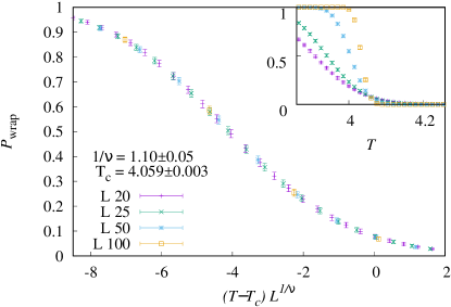
Figure 2: Wrapping probability as function of temperature $T$ for $p=0.1$, for various system sizes $L$. The inset shows the raw data, while in the main plot a data collapse to determine $T_{\rm FK}$ and $\nu$ gives $1/\nu=1.10(5)$ and $T_{\rm FK}=4.059(3)$.

In a similar way, we analysed the data for other values of $p$. The resulting values of $T_{\rm FK}$ as a function of $p$ are shown in the phase diagram in Fig. 1, along with the values for the FM-PM and SG-PM phase transitions obtained from the literature Reger and Zippelius (1986); Hasenbusch et al. (2007), and the critical concentration $p_{c}$ for the zero-temperature FM-SG transition.Hartmann (1999) Interestingly, the FK percolation transition seems to coincide with magnetic-ordering transition only for the pure ferromagnetic system ($p=0$). For all other values of $p$, $T_{c}<T_{\rm FK}$ even close to the pure ferromagnet. Hence, even if the ground state is ferromagnetic, i.e. for $0<p<p_{\rm c}$, the FM-PM phase transition cannot be understood as a percolation transition of the FK clusters.

The resulting values of $\nu$ as a function of $p$ are shown in Fig. 3. For $p=0$, we recover the literature value for the pure Ising ferromagnet,Baillie et al. (1992) but with larger error bars (which is natural, because our main numerical effort goes into the necessary disorder average and considering several values of $p$). For all other values of $p$, including both ferromagnetic and spin glass regions, we find that $\nu$ is compatible with the previously foundde Arcangelis et al. (1991) value of $\nu=0.88(5)$. This is also compatible with the valueWang et al. (2013) for the standard percolation problem, in which there are no correlations between the occupancies of the bonds. By contrast, in FT clusters there are correlations for all $p$ but interestingly they do not seem to affect the critical behavior, except for $p=0$ where the bond occupancies are rigorously constrained to follow Ising correlations.

Figure 3: The critical exponent $\nu$ as a function of $p$. The value of $\nu$ for $p=0$ is from Ref. [Baillie et al., 1992] and the value for $p=0.5$ indicated by a triangle is from Ref. [de Arcangelis et al., 1991].

To investigate universality more carefully we have evaluated the other critical exponents with additional data near $T_{\rm FK}$ for the values $p=0$ (for a consistency check), $p=0.1$ (a ferromagnetic case), $p=0.3$ and $p=0.5$ (SG cases; for the latter value the critical behavior is already partially knownde Arcangelis et al. (1991)).

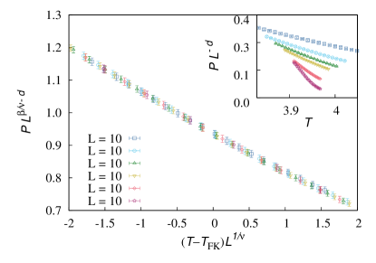
Figure 4: (color online) The fraction of sites in the infinite cluster, $P$, as a function of the temperature $T$ in the vicinity of $T_{\rm FK}$, for $p=0.3$ and various system sizes $L$. The inset shows the raw data, while the main plot shows the data rescaled according to Eq. (3), with best fitting values $\beta=0.48(4)$, $\nu=0.87(8)$, and $T_{\rm FK}=3.939(3)$.

For the fraction of sites in the infinite cluster (the order parameter), we show data for $p=0.3$ in Fig. 4. From a finite-size scaling collapse of the data we obtain the best fitting parameters $\beta=0.48(4)$, $\nu=0.87(8)$ and $T_{\rm FK}=3.939(3)$. The result for the other intensively studied cases are shown in Table 1. Note that for $T_{\rm FK}$ and $\nu$, we usually have several independent estimates available and the stated values and their error bars are chosen such that they are compatible with all results.

Table 1: Best estimates for the critical temperatures $T_{\rm FK}$ and critical exponents $\nu$, $\tau$, $\gamma$ and $\beta$. The number in brackets denote the error bars in the last digit. Also shown are the values for $\gamma$ and $\beta$ obtained by inserting the values for $\nu$ and $\gamma$ into the scaling relations in Eq. (9). They agree with the values for $\gamma$ and $\beta$ obtained directly within the error bars.

$p$	$T_{\rm FK}$	$\nu$	$\tau$	$\gamma$	$\beta$	$\gamma=\frac{3-\tau}{\tau-1}\nu d$	$\beta=\frac{\tau-2}{\tau-1}\nu d$
0.0	4.5116(5)	0.65(4)	2.27(3)	1.18(6)	0.31(4)	1.1(2)	0.4(1)
0.1	4.059(3)	0.89(8)	2.196(8)	1.82(8)	0.48(4)	1.79(12)	0.44(4)
0.3	3.941(3)	0.89(8)	2.23(5)	1.84(6)	0.41(4)	1.7(2)	0.49(16)
0.5	3.934(3)	0.88(9)	2.26(1)	1.8(1)	0.41(5)	1.6(2)	0.54(9)

In addition to the order parameter, we have also analysed the data for the average cluster size $S$. As example, we show the result for $p=0.1$ and size $L=50$ as a function of temperature $T$ in Fig. 5. The data exhibits a peak at some point ($T^{\star},S^{\star}$). One can read off the critical exponent $\gamma$ from the $L^{\gamma/\nu}$ scaling, see Eq. (5), of the peak height as a function of $L$. The data is shown in the inset of Fig. 5. For different values of $p$, the resulting values of $\gamma$ are also shown in Table 1. Again, we observe that for $p>0$ the results seem to agree with each other.

Figure 5: Mean cluster size $S$ at $L=50$ and $p=0.1$ as a function of temperature $T$, near the FK percolation transition $T_{\rm FK}$. The data exhibits a peak with peak height $S^{\star}$. The inset shows the peak height as function of $L$.

To obtain the critical exponent $\tau$, we analyse the distribution of cluster sizes, excluding the largest cluster, at the critical point for a rather large system size, $L=200$. As an example, we present our results for $p=0.3$ in Fig. 6. The data exhibits a high quality which allows us to observe a power law over about 10 decades in probability. A fit resulted in a value $\tau=2.23(5)$. This value, and the results for the three other selected cases, are also shown in Table 1. The values we have found for all values of $p>0$ are compatible with the values for standard percolation in three dimensions.

Figure 6: Cluster size distribution at $p=0.3$ with a system size of $N=200^{3}$.

The exponents should obey the scaling relations in Eqs. (9). The values obtained when inserting the measured values for $\nu$ and $\tau$ from Table 1 to estimate $\gamma$ and $\beta$ from the scaling relations are shown in the last two columns in Table 1. All these values are compatible with the directly measured values within error bars. Note that the error bars from the scaling relations are larger than the error bars of the directly measured exponents due to error propagation.

Finally we consider the question of whether the Wolff algorithm might be more efficient in the spin-glass phase near the FM-SG transition, i.e. for $p$ just slightly greater than $p_{c}$, rather than for $p=1/2$. In Fig. 7 we show the average effective size of the flipped cluster (which is not always the largest one), as a function of the temperature $T$ for $p=0.25\,(>p_{\rm c})$. By “effective” we mean that if the cluster of flipped spins is larger than half of the system size, then the spins which are not flipped are counted. We see that the clusters which are flipped near the SG phase transition are very small. One could already expect this from the phase diagram in Fig. 1, which shows that for $p=0.25$ the FK percolation transition is considerably above the critical temperature $T_{\rm SG}$. Thus, applying the Wolff algorithm in the spin glass phase but near the spin glass-ferromagnet phase boundary, does not lead to any benefit relative to studying the standard spin glass model which has $p=1/2$.

Figure 7: Average size of the clusters flipped (or not flipped if this is smaller) by the Wolff algorithm as a function of temperature $T$ for $L=10$ and $p=0.25$.

IV Summary

We have studied the percolation transitions of Fortuin-Kasteleyn clusters for the three-dimensional random-bond Ising model. Near the cluster percolation transition the Wolff algorithm can be used to efficiently sample equilibrium configurations. However, except for the pure Ising case ($p=0$), the temperature of the percolation transition is higher that of the ferromagnet-paramagnet and spin glass-paramagnet transitions, and for most values of $p$ it is much higher, see Fig. 1. This renders the Wolff algorithm inefficient for the magnetic transitions except for $p=0$. Indications of this behaviour were already found in some test simulations of a previous study,Hasenbusch et al. (2007) where, for the FM-PM phase boundary at one value of $p>0$, cluster algorithms were tried but turned out to be inefficient.

We have determined the critical exponents at the FK cluster percolation transition. For $p=0$, the pure Ising case, we obtain the known values, which are those of the Ising model since the FK clusters are controlled by Ising correlations in this limit. For all other values, $0<p\leq 1/2$, our results are compatible with the universal behaviour of standard percolation, irrespective of whether the ground state exhibits ferromagnetic or spin-glass order. Since standard percolation has no correlations between the occupancy of the bonds, whereas bonds in the FK clusters are correlated, this implies that the correlations are irrelevant for universal properties, and so presumably are of short range for $p>0$.

For future studies, it would be interesting to investigate other types of cluster algorithms Niedermayer (1988); Jörg (2005); Zhu et al. (2015) for the three-dimensional random-bond Ising model. So far, from the literature studies known to us, none of them turned out to be efficient enough to study the pure spin-glass case ($p=1/2$) for large enough systems, but it could be that some will work well close to the FM-SG phase boundary or perhaps at least for ferromagnetic ordering of the random ($p>0$) case.

V Acknowledgements

APY thanks the Alexander von Humboldt Foundation for financial support through a Research Award. The simulations were performed at the HPC facilities GWDG Göttingen, HERO and CARL. HERO and CARL are both located at the University of Oldenburg (Germany) and funded by the DFG through its Major Research Instrumentation Programme (INST 184/108-1 FUGG and INST 184/157-1 FUGG) and the Ministry of Science and Culture (MWK) of the Lower Saxony State.

References

- Binder and Young (1986) K. Binder and A. Young, Rev. Mod. Phys. 58, 801 (1986).
- Mézard et al. (1987) M. Mézard, G. Parisi, and M. Virasoro, Spin glass theory and beyond (World Scientific, Singapore, 1987).
- Young (1998) A. P. Young, ed., Spin glasses and random fields (World Scientific, Singapore, 1998).
- Nishimori (2001) H. Nishimori, Statistical Physics of Spin Glasses and Information Processing: An Introduction (Oxford University Press, Oxford, 2001).
- Ising (1925) E. Ising, Z. f. Physik 31, 253 (1925), ISSN 0044-3328, URL https://doi.org/10.1007/BF02980577.
- Hartmann (2015) A. K. Hartmann, Big Practical Guide to Computer Simulations (World Scientific, Singapore, 2015).
- Hartmann and Rieger (2001) A. K. Hartmann and H. Rieger, Optimization Algorithms in Physics (Wiley-VCH, Weinheim, 2001).
- Landau and Binder (2000) D. P. Landau and K. Binder, Monte Carlo Simulations in Statistical Physics (Cambridge University Press, Cambridge, 2000).
- Newman and Barkema (1999) M. E. J. Newman and G. T. Barkema, Monte Carlo Methods in Statistical Physics (Clarendon Press, Oxford, 1999).
- Swendsen and Wang (1987) R. H. Swendsen and J.-S. Wang, Phys. Rev. Lett. 58, 86 (1987).
- Wolff (1989) U. Wolff, Phys. Rev. Lett. 62, 361 (1989).
- Fortuin and Kasteleyn (1972) C. M. Fortuin and P. W. Kasteleyn, Physica 57, 536 (1972).
- Stauffer and Aharony (1994) D. Stauffer and A. Aharony, Introduction To Percolation Theory (Taylor & Francis, 1994), ISBN 9781420074796, URL https://books.google.de/books?id=v66plleij5QC.
- Coniglio and Klein (1980) A. Coniglio and W. Klein, J. Phys. A 13, 2775 (1980), URL https://doi.org/10.1088%2F0305-4470%2F13%2F8%2F025.
- Kessler and Bretz (1990) D. Kessler and M. Bretz, Phys. Rev. B 41, 4778 (1990).
- de Arcangelis et al. (1991) L. de Arcangelis, A. Coniglio, and F. Peruggi, EPL (Europhysics Letters) 14, 515 (1991), URL http://stacks.iop.org/0295-5075/14/i=6/a=003.
- Niedermayer (1988) F. Niedermayer, Phys. Rev. Lett. 61, 2026 (1988), URL https://link.aps.org/doi/10.1103/PhysRevLett.61.2026.
- Liang (1992) S. Liang, Phys. Rev. Lett. 69, 2145 (1992).
- Houdayer (2001) J. Houdayer, Eur. Phys. J. B 22, 479 (2001).
- Jörg (2005) T. Jörg, Progr. Theor. Phys. Suppl. 157, 349 (2005).
- Zhu et al. (2015) Z. Zhu, A. J. Ochoa, and H. G. Katzgraber, Phys. Rev. Lett. 115, 077201 (2015), URL https://link.aps.org/doi/10.1103/PhysRevLett.115.077201.
- Geyer (1991) C. Geyer, in 23rd Symposium on the Interface between Computing Science and Statistics (Interface Foundation North America, Fairfax, 1991), p. 156.
- Hukushima and Nemoto (1996) K. Hukushima and K. Nemoto, J. Phys. Soc. Jpn. 65, 1604 (1996).
- Belletti et al. (2009) F. Belletti, M. Cotallo, A. Cruz, L. A. Fernandez, A. Gordillo-Guerrero, M. Guidetti, A. Maiorano, F. Mantovani, E. Marinari, V. Martin-Mayor, et al., Comput. Sci. Eng. 11, 48 (2009).
- Kirkpatrick (1977) S. Kirkpatrick, Phys. Rev. B 16, 4630 (1977), URL https://link.aps.org/doi/10.1103/PhysRevB.16.4630.
- Reger and Zippelius (1986) J. D. Reger and A. Zippelius, Phys. Rev. Lett. 57, 3225 (1986), URL http://link.aps.org/doi/10.1103/PhysRevLett.57.3225.
- Hasenbusch et al. (2007) M. Hasenbusch, F. P. Toldin, A. Pelissetto, and E. Vicari, Phys. Rev. B 76, 094402 (2007), URL https://link.aps.org/doi/10.1103/PhysRevB.76.094402.
- Hartmann (1999) A. K. Hartmann, Phys. Rev. B 59, 3617 (1999).
- Houdayer and Hartmann (2004) J. Houdayer and A. K. Hartmann, Phys. Rev. B 70, 014418 (2004), URL https://link.aps.org/doi/10.1103/PhysRevB.70.014418.
- Melchert (2009) O. Melchert (2009), (arXiv:0910.5403v1).
- Baillie et al. (1992) C. F. Baillie, R. Gupta, K. A. Hawick, and G. S. Pawley, Phys. Rev. B 45, 10438 (1992), URL https://link.aps.org/doi/10.1103/PhysRevB.45.10438.
- Wang et al. (2013) J. Wang, Z. Zhou, W. Zhang, T. M. Garoni, and Y. Deng, Phys. Rev. E 87, 052107 (2013), URL https://link.aps.org/doi/10.1103/PhysRevE.87.052107.