Effective Coefficient Asymptotics of Multivariate Rational Functions via Semi-Numerical Algorithms for Polynomial Systems

Abstract

The coefficient sequences of multivariate rational functions appear in many areas of combinatorics. Their diagonal coefficient sequences enjoy nice arithmetic and asymptotic properties, and the field of analytic combinatorics in several variables (ACSV) makes it possible to compute asymptotic expansions. We consider these methods from the point of view of effectivity. In particular, given a rational function, ACSV requires one to determine a (generically) finite collection of points that are called critical and minimal. Criticality is an algebraic condition, meaning it is well treated by classical methods in computer algebra, while minimality is a semi-algebraic condition describing points on the boundary of the domain of convergence of a multivariate power series. We show how to obtain dominant asymptotics for the diagonal coefficient sequence of multivariate rational functions under some genericity assumptions using symbolic-numeric techniques. To our knowledge, this is the first completely automatic treatment and complexity analysis for the asymptotic enumeration of rational functions in an arbitrary number of variables.

Keywords: Analytic Combinatorics in Several Variables, Asymptotic Enumeration, Kronecker Representation, Symbolic-Numeric Algorithms

1 Introduction

1.1 Analytic Combinatorics

Analytic combinatorics is a powerful technique to compute the asymptotic behaviour of univariate sequences of complex numbers $(f_{k})_{k\geq 0}$ when the generating function of the sequence, $F(z):=\sum_{k\geq 0}f_{k}z^{k}$, is analytic in a neighbourhood of the origin. The sequence is recovered by a Cauchy integral

$$f_{k}=\frac{1}{2\pi i}\int_{C}\frac{F(z)}{z^{k}}\cdot\frac{dz}{z},$$ (1)

where $C$ is any counter-clockwise circle sufficiently close to the origin. The asymptotic analysis of this integral as $k$ tends to $\infty$ is then obtained by deforming the contour of integration so that it gets closer to the singularities of minimal modulus (called dominant singularities). This process relates the asymptotic behaviour of the sequence $(f_{k})$ to the local behaviour of its generating function $F(z)$ near these singularities. In particular, in the very frequent case where the generating function has finitely many singularities in the complex plane and at each dominant singularity $\rho$ the function admits a local expansion as a sum of monomials of the form

$$C(1-z/\rho)^{\alpha}\log^{r}\frac{1}{1-z/\rho},\quad z\rightarrow\rho,$$

with $r\in\mathbb{N}$, then each such monomial with $\alpha\in\mathbb{C}\setminus\mathbb{N}$ contributes

$$\frac{C}{\Gamma(-\alpha)}\rho^{-k}k^{-\alpha-1}\log^{r}k\,(1+\dotsb),\quad k\rightarrow\infty$$ (2)

to the asymptotic behaviour of the coefficients (the ellipsis ‘$\dotsb$’ above corresponds to a full asymptotic expansion given by Jungen [34]). When $\alpha\in\mathbb{N}$ and $r\neq 0$, a simpler formula is available; the terms with $r=0,\alpha\in\mathbb{N}$ do not contribute. Summing these contributions over all dominant singularities gives arbitrarily many terms of the asymptotic expansion of $f_{k}$ as $k\rightarrow\infty$.

In many cases, the combinatorial or probabilistic origin of the sequence translates into simple equations for $F(z)$, from where location of singularities and local behaviour can be computed. This is the heart of analytic combinatorics, for which we refer to the now standard book of Flajolet and Sedgewick [23], where the theory is introduced in detail, with proper handling of singular behaviour more general than (2), along with many illuminating examples.

1.2 Analytic Combinatorics in Several Variables (ACSV)

Over a series of recent papers culminating in a textbook compiling their results, Pemantle and Wilson [54, 55, 56, 57] and their collaborators have developed a theory of analytic combinatorics in several variables. Our aim in this work is to automate some of this theory and analyze the complexity of this approach.

To a multivariate sequence $(f_{i_{1},\dots,i_{n}})_{(i_{1},\dots,i_{n})\in\mathbb{N}^{n}}$ is associated a multivariate generating function

$$F(\mathbf{z})=F(z_{1},\dots,z_{n})=\sum_{(i_{1},\dots,i_{n})\in\mathbb{N}^{n}}f_{i_{1},\dots,i_{n}}z_{1}^{i_{1}}\cdots z_{n}^{i_{n}}=\sum_{\mathbf{i}\in\mathbb{N}^{n}}f_{\mathbf{i}}\mathbf{z}^{\mathbf{i}}.$$

As in the univariate case, when this function is analytic in the neighbourhood of the origin, now in $\mathbb{C}^{n}$, the coefficient sequence is recovered by a Cauchy integral,

$$f_{i_{1},\dots,i_{n}}=\frac{1}{(2\pi i)^{n}}\int_{T}\frac{F(\mathbf{z})}{z_{1}^{i_{1}}\dotsm z_{n}^{i_{n}}}\cdot\frac{dz_{1}\cdots dz_{n}}{z_{1}\cdots z_{n}},$$

where the domain of integration $T$ is now a polytorus sufficiently close to the origin; i.e., a product of sufficiently small circles. The asymptotic analysis of the multivariate sequence of coefficients is turned into a problem of univariate asymptotics by selecting diagonal rays in the index space: the vector $(i_{1},\dots,i_{n})/(i_{1}+\dots+i_{n})$ varies in a neighbourhood of a fixed direction. In our work, we restrict further to the main diagonal where $i_{1}=\dots=i_{n}$, but it is important to note that the theory brings insight on the uniformity of these results with respect to the direction. Even under these restrictions, the asymptotic analysis is made significantly more delicate than in the univariate case by topological issues related to how the domain of integration can be deformed in $\mathbb{C}^{n}$ while avoiding the singularities of the integrand. Pemantle and Wilson show that an important part is played by those singularities of $F$ that are critical points of the map

$$\operatorname{Abs}:(z_{1},\dots,z_{n})\mapsto|z_{1}\dotsm z_{n}|,$$

on the set of singularities of $F$ (precise definitions are given in Section 2). Among those critical points, one has to determine the minimal ones, which lie on the boundary of the domain of convergence of the generating function. The determination of these minimal critical points is the main focus of the present work.

1.3 Rational Functions and their Diagonals

In order to automate this approach in computer algebra, we first restrict the class of functions and sequences under consideration and study only multivariate rational generating functions: $F(\mathbf{z})=G(\mathbf{z})/H(\mathbf{z})$ with $G$ and $H$ polynomials in $\mathbb{Z}[z_{1},\dots,z_{n}]$ and $H(\mathbf{0})\neq 0$. One motivation is that all the tools of computer algebra related to polynomial systems become available to us. Another motivation comes from structural properties. The generating function of the diagonal coefficients is a classical object called the diagonal of $F$, denoted $\Delta F$ and defined by:

$$\Delta F(t):=\sum_{k\geq 0}{f_{k,\dots,k}t^{k}}.$$

Diagonals of rational functions in $\mathbb{Q}(\mathbf{z})$ form an important class of power series that contains the algebraic power series [24] and is contained in the set of differentially finite power series [17]; these are the power series solutions of linear differential equations with polynomial coefficients. Among differentially finite power series, diagonals of rational power series enjoy special properties: all their singularities are regular with rational exponents [35, 18, 1]. This implies that the asymptotic expansion of their coefficients is a linear combination of expressions of the form $C^{k}k^{\alpha}\log^{p}k$, with $C$ an algebraic number, $\alpha$ a rational number and $p$ a non-negative integer. Despite these special properties, a conjecture of Christol [16, Conjecture 4] asserts that the generating functions of univariate integer sequences having a finite nonzero radius of convergence and satisfying a linear differential equation with polynomial coefficients are all diagonals of rational functions. Thus, diagonals of rational functions form an important class from the point of view of applications.

For generic rational functions, the critical points mentioned above are obtained as solutions of a system of polynomial equations

$$H=z_{1}\frac{\partial H}{\partial z_{1}}=z_{2}\frac{\partial H}{\partial z_{2}}=\dots=z_{n}\frac{\partial H}{\partial z_{n}}.$$ (3)

In the most common situations considered in this article, we can avoid the use of amoebas and Morse theory that are developed by Pemantle and Wilson in their most recent works. Instead, the computations are reduced to problems of complex roots of polynomial systems such as (3) for the determination of critical points, and real roots of polynomial systems with inequalities for the selection of the minimal ones.

1.4 Combinatorial Case

We start with a special case that often arises in practice, and where determining the minimal critical points is greatly simplified. A rational function $F(\mathbf{z})$ is called combinatorial if every coefficient of its power series expansion is non-negative. This usually occurs when the rational function has been obtained by a combinatorial process. In general, it cannot be detected automatically a priori. Indeed, even in the univariate case, the question of nonnegativity of the sequence of Taylor coefficients of a rational function is only conjectured to be decidable in general [52, 53].

Informally, our first main result is the following, which is stated precisely in Theorem 56 below and which we gave earlier without the genericity analysis [46].

Result 1.

Let $G(\mathbf{z})$ and $H(\mathbf{z})$ be polynomials in $\mathbb{Z}[z_{1},\dots,z_{n}]$ of degrees at most $d$, with coefficients of absolute value at most $2^{h}$ and assume that $H(\mathbf{0})\neq 0$. Assume that $F(\mathbf{z})=G(\mathbf{z})/H(\mathbf{z})$ is combinatorial, has a minimal critical point, and satisfies certain verifiable assumptions stated in Section 3.1, that hold generically. Then there exists a probabilistic algorithm computing dominant asymptotics of the diagonal sequence in $\tilde{O}(hd^{4n+1}+h^{3}d^{3n+3})$ bit operations. The algorithm returns three rational functions $A,B,C\in\mathbb{Z}(u)$, a square-free polynomial $P\in\mathbb{Z}[u]$ and a list $U$ of roots of $P(u)$, specified by isolating regions, such that

$$f_{k,\dots,k}=(2\pi)^{(1-n)/2}\left(\sum_{u\in U}A(u)\sqrt{B(u)}\cdot C(u)^{k}\right)k^{(1-n)/2}\left(1+O\left(\frac{1}{k}\right)\right).$$ (4)

The values of $A(u),B(u),$ and $C(u)$ can be determined to precision $2^{-\kappa}$ at all elements of $U$ in $\tilde{O}(d^{n}\kappa+h^{3}d^{3n+3})$ bit operations.

Example 1.

The sequence of Apéry numbers $A_{k}=\sum_{i=0}^{k}{\binom{k}{i}^{2}\binom{k+i}{i}^{2}}$, appearing in Apéry’s proof of the irrationality of $\zeta(3)$, is, like all multiple binomial sums, the diagonal of a rational function that can be determined algorithmically by the methods of Bostan et al. [10]. In this example, they are given for instance as the diagonal of a rational function in 4 variables:

$$\sum_{k\geq 0}A_{k}t^{k}=\Delta\left(\frac{1}{1-z(1+a)(1+b)(1+c)(1+b+c+bc+abc)}\right).$$

From there, our Maple implementation gives

> F:=1/(1-z*(1+a)*(1+b)*(1+c)*(1+b+c+b*c+a*b*c)):> A, U := DiagonalAsymptotics(numer(F),denom(F),[a,b,c,z],u,k):> evala(allvalues(subs(u=U[1],A)));

$${\color[rgb]{0,0,1}\frac{\sqrt{2}\sqrt{24+17\sqrt{2}}\,\left(17+12\sqrt{2}\right)^{k}}{8\pi^{3/2}k^{3/2}}}$$

In general, it is not possible to provide such an explicit closed form for the quantities involved in the asymptotic behaviour. The output will then be a combination of an exact symbolic representation and a precise numerical estimate.

Example 2.

In Pemantle and Wilson [56, Section 4.9], the authors study sequence alignment problems with application to molecular biology. The authors give asymptotics for a family of sequences parametrized by natural numbers $k$ and $b$; for any fixed $k$ and $b$ we can automatically recover their results. For instance, when $k=b=2$ one wants to derive asymptotics of

$$\Delta\left(\frac{x^{2}y^{2}-xy+1}{1-(x+y+xy-xy^{2}-x^{2}y+x^{2}y^{3}+x^{3}y^{2})}\right),$$

which can be shown to be combinatorial through generating function manipulations. Let $F(x,y)$ be this bivariate rational function. Running

> A, U := DiagonalAsymptotics(numer(F),denom(F),[x,y],u,k, u-x-t,t):which specifies the optional linear form $u=x+t$ to be used in the algorithm (see below for details) and simplifies the output, returns $A$ equal to

$${\color[rgb]{0,0,1}\,{\frac{\left(4\,{u}^{4}-14\,{u}^{3}+14\,{u}^{2}-2\,u+2\right)}{\sqrt{n}\sqrt{2\pi}\left(10\,{u}^{4}-40\,{u}^{3}+54\,{u}^{2}-26\,u+4\right)}\left({\frac{10\,{u}^{4}-40\,{u}^{3}+54\,{u}^{2}-26\,u+4}{4\,{u}^{4}-19\,{u}^{3}+25\,{u}^{2}-4\,u-6}}\right)^{n}\sqrt{{\frac{10\,{u}^{4}-40\,{u}^{3}+54\,{u}^{2}-26\,u+4}{4\,{u}^{4}-16\,{u}^{3}+20\,{u}^{2}-8\,u+4}}}}}$$

and $U$ equal to

$${\color[rgb]{0,0,1}[\text{RootOf}(2\_Z^{5}-10\_Z^{4}+18\_Z^{3}-13\_Z^{2}+4\_Z-2,\,1.4704170\dots)]}$$

where 366 decimal places are recorded: this is an upper bound on the accuracy needed by the algorithm to rigorously decide numerical equalities and inequalities. Asymptotics are given by evaluating $A$ at the degree 5 algebraic number defined by the single element of $U$ (which is not expressible in radicals).

1.5 Non-Combinatorial Case

We also propose an algorithm finding minimal critical points in many cases, even when combinatoriality is not assumed, at the price of an increase in complexity. Our result in that case is the following, which is stated precisely in Theorem 56 below.

Result 2.

Let $F(\mathbf{z})\in\mathbb{Z}(z_{1},\dots,z_{n})$ be a rational function with numerator and denominator of degrees at most $d$ and coefficients of absolute value at most $2^{h}$. Assuming that $F$ satisfies certain verifiable assumptions stated in Section 3.3, then $F$ admits a finite number of minimal critical points that can be determined in $\tilde{O}\left(hd^{9n+5}2^{3n}\right)$ bit operations. From there, the asymptotics of the diagonal coefficients follow with the same complexity as in Result 1.

Aside from the existence of minimal critical points, we conjecture that the assumptions on $F$ required to apply Theorem 56 in the non-combinatorial case hold generically.

1.6 Previous work

A very useful introduction to the asymptotics of sequences is given in the extensive survey by Odlyzko [50]. Here, we focus on the case of coefficients of rational functions and on effective methods.

Univariate case

Finding the asymptotic behaviour of the coefficients of a univariate rational function is equivalent to finding that of a linear recurrence with constant coefficients. Decision procedures rely on the ability to determine whether two complex algebraic numbers have the same modulus. This can be done purely algebraically, and a semi-numerical algorithm has been given by Gourdon and Salvy [29]. Some of the ingredients are common with the current work, in particular a semi-numerical approach to those types of decision problems for algebraic numbers.

Probabilistic approach

Many combinatorial sequences are given as sums of non-negative terms and several techniques are available in that case, surveyed in the classic book by de Bruijn [21]. For instance, completely explicit formulas can be derived for sums of products of binomial coefficients [44].

Given the combinatorial generating function $F(\mathbf{z})$, the normalized sequence $f_{i_{1},\dots,i_{n}}/\sum_{j_{1}+\dots+j_{n}=k}{f_{j_{1},\dots,j_{n}}}$, where $k=i_{1}+\dots+i_{n}$, is a discrete probability for which central and local limit theorems for large $k$ have been derived in the bivariate case by Bender [6] and later extended by Bender, Richmond, and Gao [7, 8, 25]. The local limit theorems are the most relevant to our discussion. Let $x_{1},\dots,x_{n}$ be real positive numbers and consider the univariate generating function $f_{\mathbf{x}}(z)=F(zx_{1},\dots,zx_{n})$. Assume that in a neighbourhood of $\mathbf{x}$, there exists an analytic root $\lambda(\mathbf{x})$ of the denominator of $f_{\mathbf{x}}$ such that the other roots have strictly larger modulus. Then, if the numerator of $F$ does not vanish in a neighbourhood of $\lambda(\mathbf{x})$ and the matrix $(x_{1}x_{j}\partial^{2}\lambda/\partial x_{i}\partial x_{j})$ is not singular, the monomials $f_{\mathbf{i}}\mathbf{x}^{\mathbf{i}}$ satisfy a local limit theorem with mean $k(x_{1}\partial\lambda/\partial x_{1},\dots,x_{n}\partial\lambda/\partial x_{n})$. Shifting the mean by choosing $\mathbf{x}$ so that this mean is on the diagonal then gives the desired asymptotic behaviour, provided that $\lambda(\mathbf{x})$ still satisfies the required assumptions. The derivatives of $\lambda$ are related to those of the denominator $H(\mathbf{z})$ of the rational function $F(\mathbf{z})$, and the equality of the coordinates above then amounts to

$$z_{1}\frac{\partial H}{\partial z_{1}}=\dots=z_{n}\frac{\partial H}{\partial z_{n}}\qquad\text{at}\quad\mathbf{z}=\mathbf{x}.$$

These are the same critical point equations as Equation (3), to which we devote most of this work. (See the precise version given by Gao and Richmond [25] in their Theorem 4, where the result is expressed in terms of a $\boldsymbol{t}$, which is what we compute and for which we give complexity estimates.) As in the case of ACSV, by restricting to the case of rational functions, we can bring in tools for computer algebra and design complete algorithms, along with a complexity analysis.

Bivariate ACSV

Similarly, Pemantle and Wilson’s analytic combinatorics in several variables apply much more generally than for combinatorial rational generating functions. In terms of algorithms, the situation is much harder. Only the case of bivariate rational functions $F(x,y)$ that are not required to be combinatorial and under a smoothness hypothesis do we have an algorithm, due to de Vries et al. [22]. It is not immediately clear how to generalize this technique beyond the bivariate case and keep it effective. While our algorithms apply in higher dimension, they work under stronger minimality assumptions on critical points.

Previous implementations

A Sage package of Raichev [58] determines asymptotic contributions of non-degenerate critical points where the zero set of $H$ is smooth or locally the transverse intersection of smooth algebraic varieties. It relies on the assumption that minimality of these points has been proved beforehand, the most difficult step of the analysis.

Creative telescoping

Another approach to the computation of these asymptotic behaviours exploits the fact that diagonals of rational functions are differentially finite. A possible starting point is to use an integral representation for the diagonal as a multidimensional residue:

$$\Delta F(t)=\frac{1}{(2\pi i)^{n-1}}\oint{F\!\left(z_{1},\dots,z_{n-1},\frac{t}{z_{1}\dotsm z_{n-1}}\right)\frac{dz_{1}\dotsm dz_{n-1}}{z_{1}\dotsm z_{n-1}}}.$$

Next, a technique called the Griffiths-Dwork method performs a succession of computations modulo a polynomial ideal. For our case of a rational function $F=G/H$, this is the ideal generated by the critical point equations (3) again. The result of this method is a linear differential equation satisfied by $\Delta F$. An efficient algorithm with arithmetic complexity in $d^{O(n)}$ has been given by Bostan et al. [9] and improved by Lairez [42].

From this differential equation, univariate singularity analysis applies, following Flajolet and Sedgewick [23, §VII.9.1]. First, the possible locations of singularities are the zeros of the leading coefficient of the equation. Next, at such a point $\rho$, since the equation is Fuchsian with rational exponents, there exists a basis of local expansions of the form

$$(z-\rho)^{\alpha}\left(\phi_{r}(z)\log^{r}\frac{1}{1-z/\rho}+\dots+\phi_{0}(z)\right),$$

where $r\in\mathbb{N}$, $\alpha\in\mathbb{Q}$ and the $\phi_{k}$ are convergent power series in powers of $(z-\rho)$ that can be computed to arbitrary order. The generating function $\Delta F$, known at the origin to arbitrary order can be analytically continued numerically to $\rho$ and its coefficients $c_{\alpha,r}$ in that basis can be computed numerically efficiently with arbitrary precision [47, 48]. From there, as outlined in §1.1, a contribution to the asymptotic expansion of $f_{k,\dots,k}$ follows for all $\alpha,r$ not in $\mathbb{N}\times\{0\}$ such that $c_{\alpha,r}\neq 0$. In the common case when the coefficient $c_{\alpha,r}$ corresponding to the dominant part of the asymptotic behaviour is nonzero, then it can be recognized to be so from a certified numerical approximation and the asymptotic behaviour follows. It has the same shape as in Equation (4), with three main differences: the constant in front is given only numerically, approximated rigorously to any fixed accuracy; the exponent is not restricted to being a half-integer; a full asymptotic expansion is easily produced. This last point in particular shows that when both methods apply, they are complementary: ACSV yields a closed-form expression for the relevant scalar factor $c_{\alpha,0}$ and from there, a full asymptotic expansion is easily computed from the differential equation derived by creative telescoping. The methods of ACSV are also capable of deriving higher order terms in the asymptotic expansion, however at a higher computational cost.

Polynomial systems

There is an extensive literature in computer algebra on the complexity of analyzing the roots of a polynomial system such as the one provided by the critical point equations (3). Our work on this system relies on ideas by a variety of authors [27, 28, 63, 40] on the use of the Kronecker representation in complex or real geometry, which go far beyond the simple systems we consider here. More precisely, we make use of the recent work of Safey El Din and Schost [61], who take into account multi-homogeneity and provide estimates on the height of the representations and the bit complexities of their algorithms. Note that as this work reached completion, a new preprint by van der Hoeven and Lecerf [66] appeared that points to the possibility of improving further the exponent of $d^{n}$ in our results, while retaining the same approach. The Kronecker representation, and similar constructions, have also appeared in the literature under the name ‘rational univariate representation’ [60, 5]. To the best of our knowledge, the connection between the good properties of the Kronecker representation in terms of bit size and the fast and precise algorithms operating on univariate polynomials had not been explored before Melczer and Salvy [46], except in the case of bivariate systems [11, 38].

1.7 Outline

This article is structured as follows. In Section 2, we give an almost self-contained introduction to Analytic Combinatorics in Several Variables at a more elementary level than in the book of Pemantle and Wilson [57]. This can serve as an introduction to the subject for combinatorialists already acquainted with analytic combinatorics in one variable. It can also be skipped by those readers who are only interested in the algorithms. They will find in Section 3 an overview of the operations that need be performed in order to compute the asymptotic behaviour. Next, in Section 4, we introduce the Kronecker representation. The results of Safey El Din and Schost [61] that we need are recalled. They are used to analyze the cost of several other operations on solutions of polynomial systems. These results are illustrated on the polynomial systems arising in ACSV. Section 5 turns to the semi-numerical part of the computation. A numerical Kronecker representation is defined and the precision required for several decision problems is analyzed. Again, these are illustrated by families of examples from ACSV. We then turn back to ACSV in Section 6, where the algorithms outlined in Section 3 can finally be specified more precisely thanks to our semi-numerical tools. Section 7 gives a few more examples and Section 8 addresses the genericity of our assumptions in the combinatorial case.

2 Analytic Combinatorics in Several Variables for Rational Functions

We give an almost self-contained introduction to the part of the theory of analytic combinatorics in several variables that we need, introducing the definitions and notation for the rest of the article. Since our algorithms only address situations where the geometry is sufficiently simple, we stick to the “surgery method” of the early works of Pemantle and Wilson [54] and avoid any mention of Morse theory so that the text is more accessible to combinatorialists already familiar with the univariate situation. We also avoid amoebas; while they give a simple understanding of some properties of domains of convergence, they introduce logarithms that we want to avoid in the computations.

2.1 Domains of convergence and minimal points

For basic properties of analytic functions in several variables, we refer to Krantz [39] and Hormander [32]. We consider a multivariate rational function $F(\mathbf{z})={G(\mathbf{z})}/{H(\mathbf{z})}$ with $G$ and $H$ co-prime polynomials and $H(\mathbf{0})\neq 0$. (A large part of the analysis holds more generally for meromorphic functions, $G$ and $H$ being co-prime analytic functions.) The Taylor expansion at the origin

$$F(\mathbf{z})=\sum_{\mathbf{i}\in\mathbb{N}^{n}}f_{\mathbf{i}}\mathbf{z}^{\mathbf{i}}$$ (5)

has a nonempty open domain of convergence $\mathcal{D}\subset\mathbb{C}^{n}$.

The main properties of the multivariate case that we use are:

• a point $\mathbf{z}:=(z_{1},\dots,z_{n})$ is in the closure $\overline{\mathcal{D}}$ of $\mathcal{D}$ if and only if the open polydisk $D(\mathbf{z}):=\{\mathbf{w}\in\mathbb{C}^{n}\mid|w_{i}|<|z_{i}|,i=1,\dots,n\}$ is a subset of $\mathcal{D}$;

• the domain $\mathcal{D}$ is logarithmically convex: if the points $\mathbf{z}=(z_{1},\dots,z_{n})$ and $\boldsymbol{\zeta}=(\zeta_{1},\dots,\zeta_{n})$ are in $\mathcal{D}$, then so are the points $(|z_{1}|^{t}|\zeta_{1}|^{1-t},\dots,|z_{n}|^{t}|\zeta_{n}|^{1-t})$ for $t\in[0,1]$.

The boundary $\partial\mathcal{D}=\overline{\mathcal{D}}\setminus\mathcal{D}$ of the domain of convergence plays an important role in the analysis. At its points, the series (5) is not absolutely convergent. The following result summarizes the relation between this boundary and the algebraic set $\mathcal{V}:=\{\mathbf{z}\in\mathbb{C}^{n}\mid H(\mathbf{z})=0\}$, which Pemantle and Wilson call the singular variety of $F$.

Lemma 3.

(i) If $\mathbf{w}\in\partial\mathcal{D}$, then there exists $\mathbf{z}\in\mathcal{V}$ in its polytorus $T(\mathbf{w}):=\{(w_{1}e^{i\theta_{1}},\dots,w_{n}e^{i\theta_{n}})\mid(\theta_{1},\dots,\theta_{n})\in\mathbb{R}^{n}\}$.

(ii) The intersection $\mathcal{V}\cap\mathcal{D}$ is empty. (iii) If $\mathbf{w}$ is in $\mathcal{V}$ and $\mathcal{V}\cap D(\mathbf{w})$ is empty, then $\mathbf{w}$ belongs to $\partial\mathcal{D}$.

Proof.

(i). If no point of $T(\mathbf{w})$ belongs to $\mathcal{V}$, then the function $F$ admits a convergent power series expansion at each of these points. As $T(\mathbf{w})$ is compact, there is a $\rho>0$ such that all these power series converge in a polydisk of radius $\rho$. These allow for an analytic continuation of $F$ in a polydisk $D((|w_{1}|(1+\rho/2),\dots|w_{n}|(1+\rho/2)))$, which implies that the power series (5) is absolutely convergent at $\mathbf{w}$, contradicting the fact that $\mathbf{w}\in\partial\mathcal{D}$.

(ii). If $\mathbf{w}\in\mathcal{V}$, then $H(\mathbf{w})=0$. If $G(\mathbf{w})\neq 0$ then $F$ is infinite at $\mathbf{w}$ and thus its Taylor series does not converge in its neighbourhood. Otherwise, up to renumbering the variables we can assume that $\partial H/\partial z_{n}\neq 0$ and then, since $H$ and $G$ are coprime, their gcd when viewed as polynomials in $\mathbb{C}(z_{1},\dots,z_{n-1})[z_{n}]$ is 1 and there exist polynomials $U$, $V$ in $\mathbb{C}[\mathbf{z}]$ and $W$ nonzero in $\mathbb{C}[z_{1},\dots,z_{n-1}]$ such that $W=UG+VH$. If there was a neighborhood of $\mathbf{w}$ where $G=H=0$ then the nonzero polynomial $W$ would be 0 in a neighborhood of $(w_{1},\dots,w_{n-1})$, but this is impossible. Thus there exists $\mathbf{w}^{\prime}$ arbitrarily close to $\mathbf{w}$, where $H(\mathbf{w}^{\prime})=0$ and $G(\mathbf{w}^{\prime})\neq 0$ and therefore $\mathbf{w}\not\in\mathcal{D}$.

(iii). The proof is similar to that of (i). At any point $\mathbf{z}$ of $D(\mathbf{w})$, the function $F$ admits an analytic continuation, which implies that the power series (5) is absolutely convergent at $\mathbf{z}$ and thus that $D(\mathbf{w})\subset\mathcal{D}$. Thus $\mathbf{w}$ is in $\overline{}\mathcal{D}$. By (ii), it is not in $\mathcal{D}$ so that it belongs to $\partial\mathcal{D}$. ∎

Thus a special role is played by points in $\partial\mathcal{D}\cap\mathcal{V}$.

Definition 4.

The elements of $\partial\mathcal{D}\cap\mathcal{V}$ are called minimal points. A minimal point $\mathbf{z}$ is called finitely minimal when its polytorus $T(\mathbf{z})$ intersects $\mathcal{V}$ in finitely many points. It is called strictly minimal when this intersection is reduced to $\{\mathbf{z}\}$. It is called smooth when the gradient $\nabla H$ does not vanish at $\mathbf{z}$.

     

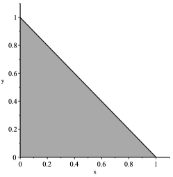
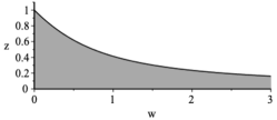
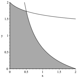
Figure 1: The gray areas give the intersections of the domains of convergence with $\mathbb{R}_{+}^{2}$ in three examples. Left: $1/(1-x-y)$; middle: $1/(1-2wz-z^{2})$; right: $1/(2+y-x(1+y)^{2})$.

Example 5.

If $F(x,y)=1/(1-x-y)$, the singular variety $\mathcal{V}$ is parameterized by $(x,1-x)$ for $x\in\mathbb{C}$. All its points are smooth: the gradient is the constant vector $(-1,-1)$. A point of $\mathcal{V}$ is minimal when there does not exist another point $(x^{\prime},y^{\prime})$ in $\mathcal{V}$ with $|x^{\prime}|<|x|$ and $|y^{\prime}|<|1-x|$. By continuity of $1/F$, it is sufficient to check that there does not exist a minimal point where one of these inequalities becomes an equality.

No point of $\mathcal{V}$ with $|x|>1$ is minimal, since for such a point, $(1,0)\in\mathcal{V}$ has smaller modulus coordinate-wise. If $|x|\leq 1$ and $x$ is not real or is negative, then $0\leq 1-|x|<|1-x|$, so that the existence of the point $(|x|,1-|x|)\in\mathcal{V}$ prevents $(x,1-x)$ from being minimal.

The conclusion is that the only possible minimal points are of the form $(x,1-x)$ with $x$ real in $[0,1]$. These are indeed minimal since any point $(x^{\prime},y^{\prime})$ with $|x^{\prime}|<x$ and $|y^{\prime}|<1-x$ satisfies $|x^{\prime}+y^{\prime}|<1$ and thus lies inside the domain of convergence. (See Figure 1, left.)

Example 6.

Consider the rational function $F(w,z)=1/(1-2wz-z^{2})$. Its singular variety $\mathcal{V}$ is parameterized by $(w(z),z)$ with $w(z)=(1-z^{2})/(2z)$ and $z\in\mathbb{C}\setminus\{0\}$. All its points are smooth: the gradient $(-2z,-2w-2z)$ does not vanish on $\mathcal{V}$.

None of those points with $|z|>1$ can be minimal: for the same value of $w$ the denominator of $F$ has another root of smaller modulus $1/|z|$. Similarly, if $|z|<1$ and $z$ it not real, then $z^{\prime}=|z|$ is such that $|1-z^{\prime 2}|<|1-z^{2}|$ so that again there is another point of $\mathcal{V}$ with smaller modulus. Finally, minimal points with $|z|=1$ must also be real: if $z=\exp(i\theta)$, then $|w(z)|=\left|\sin\theta\right|$ which is minimal when $\theta=0\bmod\pi$.

In summary, the only possible minimal points are of the form $(-u/2+1/(2u),u)$ for $u\in[-1,1]\setminus\{0\}$. These are indeed minimal as a consequence of $u\mapsto-u/2+1/(2u)$ being decreasing for positive $u$. Each of them is finitely minimal, its opposite also being in $\mathcal{V}$. (See Figure 1, middle.)

Smooth minimal points play an important part in this theory. Their role is explained by the following result.

Proposition 7 (PemantleWilson [54, Lemma 2.1] and Pemantle and Wilson [56, Prop. 3.12]).

Let $\mathbf{w}$ be a smooth minimal point. Then there exist non-negative real numbers $\lambda_{1},\dots,\lambda_{n}$, not all zero, such that:

1. $\left(w_{1}\frac{\partial H}{\partial z_{1}}(\mathbf{w}),\dots,w_{n}\frac{\partial H}{\partial z_{n}}(\mathbf{w})\right)$ and $(\lambda_{1},\dots,\lambda_{n})$ are colinear;

2. the point $\mathbf{w}$ is a local maximizer of the map $\mathbf{z}\mapsto\left|z_{1}^{\lambda_{1}}\dotsm z_{n}^{\lambda_{n}}\right|$ on $\partial\mathcal{D}$.

Proof.

Since $\mathbf{w}$ is a minimal point, the open polydisk $D(\mathbf{w})$ is included in $\mathcal{D}$ and by Lemma 3 (ii), it does not contain any element of $\mathcal{V}$. Thus the tangent lines to the torus $T(\mathbf{w})$ at $\mathbf{w}$ must belong to the tangent space to $\mathcal{V}$ at $\mathbf{w}$. Since $\nabla H$ does not vanish at $\mathbf{w}$, this leads to relations between the partial derivatives of $H$, obtained as follows.

Without loss of generality, we assume that $(\partial H/\partial z_{n})(\mathbf{w})\neq 0$. By the implicit function theorem, there exists an analytic function $g(\hat{\mathbf{z}})$ where $\hat{\mathbf{z}}:=(z_{1},\dots,z_{n-1})$, such that $(z_{1},\dots,z_{n-1},g(\hat{\mathbf{z}}))$ is a parameterization of $\mathcal{V}$ in a neighbourhood of $\mathbf{w}$: $w_{n}=g(\hat{}\mathbf{w})$, $H(\hat{\mathbf{z}},g(\hat{\mathbf{z}}))=0$ and $g$ is locally one-to-one. For any $j\in\{1,\dots,n-1\}$, differentiating $H(\hat{\mathbf{z}},g(\hat{\mathbf{z}}))=0$ with respect to $z_{j}$ yields

$$\frac{\partial H}{\partial z_{j}}(\mathbf{z})+\frac{\partial H}{\partial z_{n}}(\mathbf{z})\frac{\partial g}{\partial z_{j}}(\hat{\mathbf{z}})=0,$$

so that the vector $(\mathbf{0},1,\mathbf{0},\partial g/\partial z_{j}(\hat{}\mathbf{w}))$ with $1$ in the $j$th position lies in the tangent space to $\mathcal{V}$ at $\mathbf{w}$. In a neighbourhood of $\theta=0$, the image of $\left(\hat{}\mathbf{w},g(\hat{}\mathbf{w})\right)$ when $w_{j}$ is replaced by $w_{j}e^{i\theta}$ moves along $iw_{j}(\mathbf{0},1,\mathbf{0},\partial g/\partial z_{j}(\hat{}\mathbf{w}))$, and minimality of $|w_{n}|$ implies that this vector should be tangent to the torus; i.e., there exists a real $\lambda_{j}$ such that this vector equals $(\mathbf{0},iw_{j},\mathbf{0},-i\lambda_{j}w_{n})$. Moreover, the presence of $(\mathbf{0},w_{j},\mathbf{0},-\lambda_{j}w_{n})$ in the tangent plane to $\mathcal{V}$ at $\mathbf{w}$ implies $\lambda_{j}\geq 0$, since otherwise $\mathcal{D}$ would intersect $\mathcal{V}$. In summary, we have obtained the existence of $\lambda_{1},\dots,\lambda_{n-1},\lambda_{n}$, with $\lambda_{n}=1$, all real and non-negative, such that

$$\lambda_{n}w_{j}\frac{\partial H}{\partial z_{j}}(\mathbf{w})=\lambda_{j}w_{n}\frac{\partial H}{\partial z_{n}}(\mathbf{w}),\qquad j\in\{1,\dots,n-1\}.$$

Linear combinations give

$$\lambda_{k}w_{j}\frac{\partial H}{\partial z_{j}}(\mathbf{w})=\lambda_{k}\lambda_{j}w_{n}\frac{\partial H}{\partial z_{n}}(\mathbf{w})=\lambda_{j}w_{k}\frac{\partial H}{\partial z_{i}}(\mathbf{w}),$$

which concludes the proof of the first part of the proposition.

That each of the vectors $(\mathbf{0},i\lambda_{n}w_{j},\mathbf{0},i\lambda_{j}w_{n})$ is tangent to the torus $T(\mathbf{w})$ at $\mathbf{w}$ is equivalent to the product of $w_{j}e^{i\lambda_{j}\theta_{j}}$ for $j=1,\dots,n$ being multiplied by complex numbers of modulus 1 locally; i.e., its modulus is locally constant. It then has to be a local maximum by minimality of $\mathbf{w}$ and nonnegativity of the $\lambda_{j}$s. ∎

Example 8.

By a reasoning similar to that of the previous examples, the minimal points of the rational function $F=1/(2+y-x(1+y)^{2})$ are all smooth and of the form $((2+y)/(1+y)^{2},y)$ for $y\in[-2,-\sqrt{3}]\cup[0,\sqrt{3}]$ (See Figure 1, right.). At these points, $(x\partial H/\partial x,y\partial H/\partial y)$ is colinear to the real vector $(\lambda_{1},\lambda_{2})=(2+y,2+y-2/(1+y))$. This is never colinear to $(1,1)$, which puts this function outside of the scope of our methods, as shown in Example 14 below.

2.2 Exponential Growth

The starting point in the asymptotic analysis is a Cauchy integral representation of the diagonal coefficients: for any $k\in\mathbb{N}$,

$$f_{k,\dots,k}=\frac{1}{(2\pi i)^{n}}\int_{T}\frac{F(\mathbf{z})}{(z_{1}\cdots z_{n})^{k}}\frac{dz_{1}\cdots dz_{n}}{z_{1}\cdots z_{n}},$$ (6)

where $T$ is a polytorus sufficiently close to the origin.

The first step is to determine the exponential growth of the diagonal sequence,

$$\rho:=\limsup_{k\rightarrow\infty}|f_{k,\dots,k}|^{1/k}.$$

A consequence of the integral representation (6) is Cauchy’s inequality on the coefficients of an analytic function, implying $\rho\leq|z_{1}\cdots z_{n}|^{-1}$ for any $\mathbf{z}\in\mathcal{D}$. Then, by the maximum principle, it follows that

$$\rho\leq|z_{1}\dotsm z_{n}|^{-1},\quad\text{for any~{}$\mathbf{z}\in\partial\mathcal{D}$}$$

while by Lemma 3 (i),

$$\inf_{\mathbf{z}\in\partial D}|z_{1}\dotsm z_{n}|^{-1}=\inf_{\mathbf{z}\in\partial D\cap\mathcal{V}}|z_{1}\dotsm z_{n}|^{-1}.$$

Minimal points are those to which the cycle of integration $T$ in the Cauchy integral representation (6) may be taken arbitrarily close without changing the value of the integral. In the neighbourhood of a finitely minimal point where $|z_{1}\dotsm z_{n}|$ is maximal, the contour can be further deformed so as to capture the contribution of that point to the asymptotic behaviour of the integral. This is done in §2.4.

2.3 Critical Points

Instead of computing the set of minimal points first and then looking for those that maximize $|z_{1}\dotsm z_{n}|$, it turns out to be easier to compute a somewhat related set formed by the extrema of $|z_{1}\dotsm z_{n}|$ on subsets of $\mathcal{V}$ and then select its elements that are minimal. In many cases, those points are sufficient to complete the asymptotic analysis.

Thus the next step is to focus on the map

$$\operatorname{Abs}:\mathbf{z}\mapsto|z_{1}\dotsm z_{n}|,$$

and study its extrema on $\mathcal{V}$. These extrema can be obtained as solutions of an optimization problem for the map $\operatorname{Abs}$ from $\mathbb{R}^{2n}$ to $\mathbb{R}$, restricted to the set $\mathcal{V}$, viewed as a subset of $\mathbb{R}^{2n}$. A real-valued Lagrangian associated to this optimization problem is $L(\mathbf{z},\lambda):=\mathbf{z}\overline{\mathbf{z}}+2\Re(\lambda H(\mathbf{z}))$, where $\mathbf{z}\overline{\mathbf{z}}=z_{1}\overline{z_{1}}+\cdots+z_{n}\overline{z_{n}}$ and $\Re(w)$ denotes the real part of $w\in\mathbb{R}$. Standard arguments make it possible to work with complex derivatives only (see [64, App.2], [59, ch.1,§4], [12]): for a real valued function $f$ of $z=x+iy$ and $\overline{z}=x-iy$ that is differentiable as a function of $(x,y)$, the simultaneous vanishing of $\partial f/\partial x$ and $\partial f/\partial y$ is equivalent to the vanishing of $\partial f/\partial z=(\partial f/\partial x-i\partial f/\partial y)/2$, or equivalently to the vanishing of $\partial f/\partial\overline{z}=(\partial f/\partial x+i\partial f/\partial y)/2$.

The extrema can only be reached in three situations: either at points of $\mathcal{V}$ where one of the coordinates $z_{i}$ is 0, where $\operatorname{Abs}$ is not differentiable, or at critical points of $\operatorname{Abs}$, where either the gradient with respect to the complex coordinates $\nabla H:=(\partial H/\partial z_{1},\dots,\partial H/\partial z_{n})$ is 0 or where the optimality condition $\nabla L=0$ holds. (In this last case, the gradients $\nabla|\mathbf{z}|^{2}$ and $\nabla H$ are colinear, so that the level surface of $\operatorname{Abs}(\mathbf{z})$ is tangent to $\mathcal{V}$.)

Lemma 9.

The critical points of the map $\operatorname{Abs}:\mathbf{z}\mapsto|z_{1}\dotsm z_{n}|$ on $\mathcal{V}$ are located at solutions of the equations

$$H(\mathbf{z})=0,\qquad z_{1}\frac{\partial H}{\partial z_{1}}=\dots=z_{n}\frac{\partial H}{\partial z_{n}}.$$ (7)

Proof.

Clearly the equations hold when the gradient of $H$ is 0. The remaining case is obtained by writing out the equations for the coordinates of $\nabla L=0$. From

$$L=\mathbf{z}\overline{\mathbf{z}}+\lambda H(\mathbf{z})+\overline{\lambda H(\mathbf{z})},$$

it follows that for $i\in\{1,\dots,n\}$,

$$\frac{\partial L}{\partial z_{i}}=\frac{\mathbf{z}\overline{\mathbf{z}}}{z_{i}}+\lambda\frac{\partial H(\mathbf{z})}{\partial z_{i}}.$$

The solutions with nonzero coordinates of $\partial L/\partial z_{i}=0$ for $i=1,\dots,n$ are precisely those of Equation (7). ∎

Definition 10.

The Equations (7) are called the critical-point equations. Their solutions are called critical points, the map $\operatorname{Abs}$ being implicit. Those that do not cancel the gradient $\nabla H$ are called smooth.

Example 11.

Consider again the polynomial $H=1-x-y$ from Example 5. The critical point equations (7) reduce to $\{1-x-y=0,x=y\}$, so that they have a unique solution $x=y=1/2$, where the level surface of $|xy|$ is tangent to $\mathcal{V}$ (see Figure 2, left). This point is also minimal, as shown in Example 5.

This critical point is neither a maximum nor a minimum of $\operatorname{Abs}:\mathbf{z}\mapsto|xy|$ on $\mathcal{V}$, but only a saddle point. This can be seen either by considering the principal minors of the bordered Hessian of $L$, or directly, by observing that for small real positive $t$, the points $(1/2+t,1/2-t)$ and $(1/2+it,1/2-it)$ lie on $\mathcal{V}$, while the map $\operatorname{Abs}$ takes values $1/4-t^{2}$ and $1/4+t^{2}$ on them.

It is however a maximum of $\operatorname{Abs}$ on $\partial\mathcal{D}$. Indeed, by Lemma 3 and Example 5, the elements $(x,y)$ of $\partial\mathcal{D}\cap\mathcal{V}$ satisfy $|y|=1-|x|$, so that the maximum of $|xy|$ is reached when $|x|=|y|=1/2$.

The last feature of this example is a reflection of a more general phenomenon relating minimal critical points and maximizers of $\operatorname{Abs}$.

Lemma 12 (Pemantle and Wilson [56, Prop. 3.12]).

If $\mathbf{w}$ is a smooth minimal critical point, then it is a local maximizer of the map $\operatorname{Abs}:\mathbf{z}\mapsto|z_{1}\dotsm z_{n}|$ on $\partial\mathcal{D}$.

Proof.

Since $\mathbf{w}$ is critical, the vectors $(z_{1}\partial H/\partial z_{1},\dots,z_{n}\partial H/\partial z_{n})$ and $(1,\dots,1)$ are colinear. The conclusion follows from Proposition 7. ∎

It is important to note that it can also happen that the critical-point equations do not have any solution.

Example 13.

The generating function of Example 6 leads to the critical-point equations

$$H=1-2wz-z^{2}=0,\quad-2wz-2z^{2}=-2wz.$$

The second equation forces $z=0$, which is incompatible with the first one. There is no critical point in that case. In Figure 1 (middle), this is reflected by the fact that no level curve of $|wz|$ is tangent to the boundary of the domain of convergence.

Example 14.

Example 8 is another example of a generating function that does not have any minimal critical point. Furthermore, it does not have critical points at all: the critical-point equations are

$$H=2+y-x(1+y)^{2}=0,\quad x+y-xy^{2}=0;$$

multiplying the first equation by $1-y$, the second one by $1+y$ and adding gives $2=0$, showing that this system does not have any solution. Note however that the point $(1/2,\sqrt{3})$ is a local maximizer of $|xy|$ on $\partial\mathcal{D}$ where the critical-point equations are not satisfied.

This is due to a phenomenon shown in Figure 1 (right). Suppose $\mbox{\boldmath$\rho$}_{1}=(1/2,\sqrt{3})$ and $\mbox{\boldmath$\rho$}_{2}=(1/2,-\sqrt{3})$ are the two points in $\mathcal{V}$ with coordinate-wise moduli $(1/2,\sqrt{3})$, and let $\mathcal{N}_{1}$ and $\mathcal{N}_{2}$ be two small neighbourhoods of $\mbox{\boldmath$\rho$}_{1}$ and $\mbox{\boldmath$\rho$}_{2}$ in $\mathcal{V}$. Then $(1/2,\sqrt{3})$ is not a local maximizer of $|xy|$ on the images of $\mathcal{N}_{1}$ and $\mathcal{N}_{2}$ under $(x,y)\mapsto(|x|,|y|)$, it only becomes a local maximizer on $\partial\mathcal{D}$ because the images of $\mathcal{N}_{1}$ and $\mathcal{N}_{2}$ intersect after taking coordinate-wise moduli (Baryshnikov and Pemantle call this a ‘ghost intersection’). In particular, the level surface of $\operatorname{Abs}(x,y)$ is not tangent to $\mathcal{V}$ at either of $\mbox{\boldmath$\rho$}_{1}$ and $\mbox{\boldmath$\rho$}_{2}$.s

The critical-point equations (7) form a system of $n$ equations in $n$ unknowns. They are our starting point in this work, where we focus on the case when they have finitely many solutions, among which the minimal points have to be found. Slightly more general cases can be handled by small variations. For instance, when $H$ is not square-free, its gradient vanishes, but one can recover the relevant set of critical points by replacing $H$ with its square-free part in Equations (7). More involved geometries of $\mathcal{V}$ become difficult to analyze by elementary means. This is what led Pemantle and Wilson [57] to develop their work in the language of Morse theory.

2.4 Asymptotic Analysis

We first illustrate the main steps of the derivation on a simple example.

Example 15.

The power series $F=1/(1-x-y)$ has for diagonal

$$\Delta\left(\frac{1}{1-x-y}\right)=\sum_{k\geq 0}{\binom{2k}{k}t^{k}}=\frac{1}{\sqrt{1-4t}}.$$

The asymptotic behavior of the diagonal coefficients is easily seen to be $4^{k}/\sqrt{k\pi}$, e.g., by Stirling’s formula. The derivation of this result by ACSV starts with the integral representation

$$a_{k}=\frac{1}{2\pi i}\int_{|x|=r}\left(\frac{1}{2\pi i}\int_{|y|=r}{\frac{1}{1-x-y}\frac{dy}{(xy)^{k+1}}}\right)dx$$

for any $0<r<1/2$. For a fixed $x$ on the circle $|x|=r$, the integrand admits a unique pole, at $y=1-x$, outside of the initial circle of integration. Deforming the contour as indicated in Figure 2 (middle) shows that the integral with respect to $y$ is the sum of an integral over a contour $|y|=1/(3r)>1/2$, and the opposite of the residue at $y=1-x$, namely $1/(x(1-x))^{k+1}$. As $k$ increases, the factor $(xy)^{-k-1}$ in the integral over the large circle makes it grow exponentially like $(|xy|)^{-k}=3^{k}$. The coefficient $a_{k}$ thus behaves asymptotically like

$$a_{k}=\frac{1}{2\pi i}\oint_{|x|=r}{\frac{dx}{(x(1-x))^{k+1}}}+O(c^{k}),\qquad c<4.$$

     

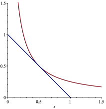
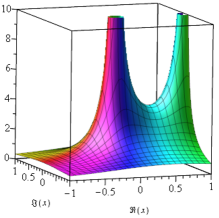
Figure 2: Example 15 in three steps: critical points where the level curve of $|xy|$ is tangent to the singular variety (left); contour of integration in the $y$-plane (middle); modulus of the integrand $1/(x(1-x))$ with a saddle point at $x=1/2$ (right).

This last integrand has a saddle point in the complex plane at $x=1/2$ (Figure 2, right), where the integral concentrates asymptotically. The classical saddle-point method (see Olver [51]) then consists in: deforming the contour so that it passes through the saddle point in the direction of the imaginary axis; changing the variable into $x=1/2+it$ and observing that the integrand behaves locally as

$$(x(1-x))^{-k-1}=4^{k+1}e^{-4(k+1)t^{2}}(1+O(t^{3})),\quad t\rightarrow 0;$$

reducing the asymptotic behaviour to that of a Gaussian integral, thus recovering the expected $4^{k}/\sqrt{k\pi}$.

The saddle-point integral in Example 15 arose because of a minimal critical point at $(1/2,1/2)$. One aspect of the computation that is missing from this simple example is the selection of those critical points that are minimal. In the context of this work, this is the most expensive step computationally. It is discussed in the next sections.

The techniques used in this example generalize. If $\boldsymbol{\zeta}\in\mathcal{V}$ is a smooth point, then as in the proof of Proposition 7, we assume without loss of generality that $(\partial H/\partial z_{n})(\boldsymbol{\zeta})\neq 0$ and introduce the implicit function $g(\hat{\mathbf{z}})$ such that $H(\hat{\mathbf{z}},g(\hat{\mathbf{z}}))=0$ and $g$ is locally one-to-one in the neighbourhood of $\boldsymbol{\zeta}$. Next, we consider

$$\psi(\hat{\mathbf{z}})=z_{1}\dotsm z_{n-1}g(\hat{\mathbf{z}}).$$

Lemma 16.

With these notations, the critical point equations are equivalent to $\nabla\psi(\hat{}\boldsymbol{\zeta})=0$.

Proof.

For $i\in\{1,\dots,n-1\}$, differentiating $H(\hat{}\mathbf{z},g(\hat{}\mathbf{z}))=0$ with respect to $z_{i}$ yields

$$\frac{\partial g}{\partial z_{i}}=-\frac{\partial H}{\partial z_{i}}\big{/}\frac{\partial H}{\partial z_{n}},$$

which can be injected into

$$\frac{1}{\psi}\frac{\partial\psi}{\partial z_{i}}=\frac{1}{z_{i}}+\frac{1}{g(\hat{}\mathbf{z})}\frac{\partial g}{\partial z_{i}},$$

and the conclusion follows from $\zeta_{n}=g(\hat{}\boldsymbol{\zeta})$. ∎

Thus locally on $\mathcal{V}$ in the neighbourhood of a smooth critical point $\boldsymbol{\zeta}$, the function $\psi$ behaves like

$$\psi(\hat{}\mathbf{z}):=\zeta_{1}\dotsm\zeta_{n}+\frac{1}{2}(\hat{}\mathbf{z}-\hat{}\boldsymbol{\zeta})^{t}\cdot\mathcal{H}(\boldsymbol{\zeta})\cdot(\hat{}\mathbf{z}-\hat{}\boldsymbol{\zeta})+O\left(\left|\hat{}\mathbf{z}-\hat{}\boldsymbol{\zeta}\right|^{3}\right),$$ (8)

where $\mathcal{H}$ is the Hessian matrix of $\psi$ (the $(n-1)\times(n-1)$ matrix whose entry $(i,j)$ is $\partial^{2}\psi/\partial z_{i}\partial z_{j}$).

Definition 17.

The critical point $\boldsymbol{\zeta}$ is called non-degenerate when the Hessian $\mathcal{H}$ of $\psi$ is non-singular at $\hat{\mathbf{z}}=\hat{\boldsymbol{\zeta}}$.

In this favourable situation, the main result of ACSV is the following.

Proposition 18.

Pemantle and Wilson [57, Theorem 9.2.7, Corollary 9.2.8] Suppose $F(\mathbf{z})$ has a smooth, strictly minimal, non-degenerate critical point with non-zero coordinates at $\boldsymbol{\zeta}$. Then the diagonal coefficients satisfy

$$f_{k,\dots,k}=\boldsymbol{\zeta}^{-k}k^{\frac{1-n}{2}}\left(\frac{(2\pi)^{(1-n)/2}}{\sqrt{(\boldsymbol{\zeta}^{3-n}/\zeta_{n}^{2})|\mathcal{H}(\boldsymbol{\zeta})|}}\cdot\frac{-G(\boldsymbol{\zeta})}{\zeta_{n}\frac{\partial H}{\partial_{z_{n}}}(\boldsymbol{\zeta})}+O\left(\frac{1}{k}\right)\right),\qquad k\rightarrow\infty,$$ (9)

where $|\mathcal{H}(\boldsymbol{\zeta})|$ is the determinant of the Hessian of $\psi$.

The branch of the square-root in Equation (9) is determined by the saddle-point integral arising in the proof of Proposition 18.

Sketch of the proof following [54].

The starting point is the Cauchy integral (6) and the idea is to first perform the integration with respect to $z_{n}$. Initially, the domain of integration is the product of the polytorus $T(\hat{}\boldsymbol{\zeta})$ and the circle $|z_{n}|=|\zeta_{n}|-\epsilon$ for a small positive $\epsilon$, so that for $\mathbf{z}$ on the contour, the open polydisk $D(\mathbf{z})$ is included in the domain of convergence of the power series (5). For $\hat{}\mathbf{z}\in T(\hat{}\boldsymbol{\zeta})$ bounded away from $\hat{}\boldsymbol{\zeta}$, the radius of convergence of $F(\hat{}\mathbf{z},z_{n})$ as a function of $z_{n}$ is larger than $|\zeta_{n}|$ as a consequence of the minimality of $\boldsymbol{\zeta}$ and thus the inner integral is bounded by $(|\zeta_{n}|+\delta)^{-k}$ for some uniform $\delta>0$, so that that part of the integral is asymptotically exponentially smaller than $|\zeta_{1}\dotsm\zeta_{n}|^{-k}$.

In the remaining part $T^{\prime}\ni\boldsymbol{\zeta}$ of the domain, since $\boldsymbol{\zeta}$ is smooth, one can use the implicit function $g$ defined above. In a sufficiently small neighbourhood of $\zeta$, the implicit function theorem even ensures that there exists a larger disk $D^{\prime}=D((1+\epsilon)\zeta_{n})$ such that the only singularity of the inner integrand inside $D^{\prime}$ with respect to the variable $z_{n}$ is the simple pole at $g(\hat{}\mathbf{z})$. There, its residue is

$$\operatorname{Res}\left(\left.\frac{G(\mathbf{z})}{H(\mathbf{z})(z_{1}\cdots z_{n})^{k+1}}\right|z_{n}=g(\hat{\mathbf{z}})\right)=\frac{G(\hat{\mathbf{z}},g(\hat{\mathbf{z}}))}{\frac{\partial H}{\partial z_{n}}(\hat{\mathbf{z}},g(\hat{\mathbf{z}}))}\frac{1}{\psi(\hat{\mathbf{z}})^{k+1}}.$$

By Cauchy’s residue theorem, the integral over $T^{\prime}\times D(|\zeta_{n}|-\epsilon)$ is thus equal to the integral over $T^{\prime}\times D(|\zeta_{n}|+\epsilon)$ minus this residue multiplied by $2\pi i$. The integral over $T^{\prime}\times D(|\zeta_{n}|+\epsilon)$ decreases asymptotically like $|\boldsymbol{\zeta}|^{-k}(1+\epsilon)^{-k}$ as $k\rightarrow\infty$, so that

$$f_{k,\dots,k}=\frac{1}{(2\pi i)^{n-1}}\int_{T^{\prime}}{\frac{-G(\hat{\mathbf{z}},g(\hat{\mathbf{z}}))}{\frac{\partial H}{\partial z_{n}}(\hat{\mathbf{z}},g(\hat{\mathbf{z}}))}\frac{dz_{1}\dotsm dz_{n-1}}{\psi(\hat{\mathbf{z}})^{k+1}}}+O\left((|\boldsymbol{\zeta}|(1+\epsilon))^{-k}\right).$$ (10)

Now, this integrand has a saddle point at $\hat{}\boldsymbol{\zeta}$, in the neighbourhood of which the integral concentrates asymptotically. There, the Taylor expansion of the integrand is

$$\frac{-G(\boldsymbol{\zeta})}{\frac{\partial H}{\partial z_{n}}(\boldsymbol{\zeta})\psi(\boldsymbol{\zeta})^{k+1}}\exp\left(-\frac{k+1}{2\psi(\boldsymbol{\zeta})}(\hat{}\mathbf{z}-\hat{}\boldsymbol{\zeta})^{t}\cdot\mathcal{H}(\boldsymbol{\zeta})\cdot(\hat{}\mathbf{z}-\hat{}\boldsymbol{\zeta})+O\left(\left|\hat{}\mathbf{z}-\hat{}\boldsymbol{\zeta}\right|^{3}\right)\right).$$

Since $\mathcal{H}$ is non-singular, the integrand behaves locally like a Gaussian integral and saddle-point methods can be applied to obtain asymptotics (see Wong [69]). ∎

All the proofs up to this point reduce to deformations of univariate integrals. A genuinely multivariate deformation of the contour makes it possible to avoid $\mathcal{V}$ while extending the domain of integration beyond the minimal points that are not critical, leading to the following.

Proposition 19 (Baryshnikov and Pemantle [3]).

If the point $\boldsymbol{\zeta}$ of the previous proposition is not necessarily strictly minimal but $T(\boldsymbol{\zeta})$ contains only a finite number of critical points, all of them being smooth and non-degenerate, then asymptotics of the diagonal coefficients of $F(\mathbf{z})$ are obtained by summing up the contributions (9) given by each of these points.

Note that one can apply Proposition 18 using any coordinate $z_{k}$ such that $(\partial H/\partial z_{k})(\boldsymbol{\zeta})\neq 0$, and in the context of Proposition 19, this coordinate may change depending on the minimal critical point under consideration.

When the numerator $G(\mathbf{z})$ is 0 at the strictly minimal critical point $\boldsymbol{\zeta}$ then Equation (9) gives only an order bound on the asymptotics of the diagonal sequence. Generically the numerator does not vanish at the critical points of $F$, however when this does happen one can typically determine dominant asymptotics by computing further terms of the Taylor expansion for $G(\mathbf{z})$ in a neighbourhood of $\boldsymbol{\zeta}$.

The Hessian $\mathcal{H}(\boldsymbol{\zeta})$ in Equation (9) can be expressed in terms of that of $H$ itself. For a critical point $\boldsymbol{\zeta}$, define $\lambda$ to be the common value of $\zeta_{k}(\partial H/\partial z_{k})(\boldsymbol{\zeta})$ ($1\leq k\leq n$) and for $1\leq k,\ell\leq n$, set

$$U_{k,\ell}:=\zeta_{k}\zeta_{\ell}\frac{\partial^{2}H}{\partial z_{k}\partial z_{\ell}}(\boldsymbol{\zeta}).$$ (11)

Basic multivariate calculus shows that the $(n-1)\times(n-1)$ Hessian matrix $\mathcal{H}$ at $\boldsymbol{\zeta}$ has $(i,j)^{\text{th}}$ entry

$$\mathcal{H}_{i,j}=\begin{cases}\frac{\zeta_{1}\cdots\zeta_{n}}{\lambda\zeta_{i}\zeta_{j}}(U_{i,n}+U_{j,n}-U_{i,j}-U_{n,n}-\lambda)&\text{if $i\neq j$,}\\[5.69054pt] \frac{\zeta_{1}\cdots\zeta_{n}}{\lambda\zeta_{i}^{2}}(2U_{i,n}-U_{i,i}-U_{n,n}-2\lambda)&\text{if $i=j$.}\end{cases}$$ (12)

This makes it simple to compute the asymptotic contribution (9) at a non-degenerate minimal critical point $\boldsymbol{\zeta}$.

2.5 Combinatorial Case

The determination of the minimal points among the critical points is significantly easier when further positivity conditions hold.

Definition 20.

A rational function $F(\mathbf{z})={G(\mathbf{z})}/{H(\mathbf{z})}$ with $H(\mathbf{0})\neq 0$ is called combinatorial when the coefficients of its Taylor expansion at the origin are all non-negative.

In these conditions, the following result is a multivariate variant, that actually extends to meromorphic functions, of a classical theorem in the univariate case usually attributed to one of Pringsheim, Borel or Vivanti, see [30, 67]. (Pemantle and Wilson [57, Prop. 8.4.3] give a stronger statement.)

Lemma 21.

If $F(\mathbf{z})$ is combinatorial and $\mathbf{w}$ belongs to the boundary $\partial\mathcal{D}$ of its domain of convergence, then the point $|(\mathbf{w})|=(|w_{1}|,\dots,|w_{n}|)$ is minimal. If moreover $\mathbf{w}$ is smooth and critical, then $|(\mathbf{w})|$ is critical too.

Note that the hypothesis can be weakened to allow a finite number of negative coefficients in the Taylor series of $F(\mathbf{z})$, by subtracting the corresponding polynomial.

Proof.

Since $\mathbf{w}$ belongs to the boundary of the domain of convergence, the Taylor expansion of $F$ does not converge absolutely as $\mathbf{z}$ tends to $\mathbf{w}$ inside $D(\mathbf{w})$. Non-negativity of the coefficients then implies that the Taylor expansion of $F$ does not converge as $\mathbf{z}$ tends to $(|w_{1}|,\dots,|w_{n}|)$ inside $D(\mathbf{w})$. Since the function is meromorphic, this implies that it tends to $\infty$ and that that point is a zero of $H$. It is therefore both on the boundary of the domain of convergence and on $\mathcal{V}$, as was to be proved.

If $|(\mathbf{w})|$ is not smooth, then it is critical. Otherwise, by Proposition 7, there exists $\boldsymbol{\lambda}=(\lambda_{1},\dots,\lambda_{n})$ with non-negative real coordinates such that $(|w_{1}|\partial H/\partial z_{1}(|(\mathbf{w})|),\dots,|w_{n}|\partial H/\partial z_{n}(|(\mathbf{w})|))$ and $\boldsymbol{\lambda}$ are colinear and $|(\mathbf{w})|$ is a local maximizer of the map $\operatorname{Abs}_{\boldsymbol{\lambda}}:\mathbf{z}\mapsto|z_{1}^{\lambda_{1}}\dotsm z_{n}^{\lambda_{n}}|$ on $\partial\mathcal{D}$. It remains to show that $\boldsymbol{\lambda}=(1,\dots,1)$. If not, there exists $\mathbf{v}\in\mathbb{R}^{n}$ such that $\mathbf{v}\cdot(1,\dots,1)=0$ and $\mathbf{v}\cdot\boldsymbol{\lambda}>0$. Since $\mathbf{w}$ is smooth and critical, by Lemma 12 it is a local maximizer of $\operatorname{Abs}$ on $\partial\mathcal{D}$. Note that for small enough $\epsilon>0$, the point $(w_{1}e^{\epsilon v_{1}},\dots,w_{n}e^{\epsilon v_{n}})$ belongs to $\overline{\mathcal{D}}$. Then so does $(|w_{1}|e^{\epsilon v_{1}},\dots,|w_{n}|e^{\epsilon v_{n}}),$ but this contradicts the local maximality of $(|\mathbf{w}|)$ for $\operatorname{Abs}_{\boldsymbol{\lambda}}$. ∎

The first part of this result is the basis of the following test leading to an efficient algorithm in the next section.

Proposition 22.

If $F$ is combinatorial and $\mathbf{w}$ is in $\mathcal{V}$, then $\mathbf{w}$ is a minimal point if and only if the line segment $\{(t|w_{1}|,\dots,t|w_{n}|):0<t<1\}$ does not intersect $\mathcal{V}$.

Proof.

One direction is straightforward and does not depend on $F$ being combinatorial: if $\mathbf{w}$ is minimal, its polydisk $D(\mathbf{w})$ is a subset of the domain of convergence, so that it cannot contain any point $(t|w_{1}|,\dots,t|w_{n}|)\in\mathcal{V}$ with $t\in(0,1)$ by Lemma 3 (ii).

Conversely, let $\mathbf{w}$ be in $\mathcal{V}$, assume that the line segment of the proposition does not intersect $\mathcal{V}$ and let

$$\mathcal{S}:=\{t\geq 0\mid(t|w_{1}|,\dots,t|w_{n}|)\in\mathcal{D}\}.$$

Since $H(\mathbf{0})\neq 0$ the set $\mathcal{S}$ is not empty. It is also included in $(0,1)$ since $\mathbf{w}$ is a singularity of $F$. Thus $\theta:=\sup\mathcal{S}$ is well defined and finite. The point $\theta|\mathbf{w}|:=(\theta|w_{1}|,\dots,\theta|w_{n}|)$ belongs to $\partial D$. This means that its torus intersects $\mathcal{V}$, by Lemma 3 and by the previous lemma that $\theta|\mathbf{w}|$ itself belongs to $\mathcal{V}$. The hypothesis then implies $\theta=1$ and thus that $\mathbf{w}$ is minimal. ∎

Example 23.

The generating function of Example 1, whose diagonal coefficients are the Apery numbers, is combinatorial. The critical-point equations are

$$H(a,b,c,z)=1-z(1+a)(1+b)(1+c)(1+b+c+bc+abc)=0,$$

$$\begin{aligned} z(1+a)(1+b)(1+c)(1+b+c+bc+abc)&=az(1+b)(1+c)(1+b+c+2bc+2abc)\\ &=bz(1+a)(1+c)(2+2b+2c+ac+2bc+2abc)\\ &=cz(1+a)(1+b)(2+2b+2c+ab+2bc+2abc).\end{aligned}$$

They have only two solutions with $abc\neq 0$: $a=1\pm\sqrt{2},b=\pm{\sqrt{2}}/2,c=\pm{\sqrt{2}}/{2},z=-82\pm 58\sqrt{2}$. Only the solution with $+\sqrt{2}$ has non-negative coordinates so that it is the only one that is possibly minimal. Adding the equation $H(ta,tb,tc,tz)=0$, eliminating the variables $a,b,c,z$ and discarding the point $t=1$ produces the polynomial

$$t^{12}-2t^{11}+t^{10}+4t^{9}-24t^{8}-8t^{7}+20t^{6}-20t^{5}+212t^{4}-400t^{3}+820t^{2}-664t-4$$

with no root in the interval $(0,1)$. This proves the minimality of that solution.

Proposition 24.

If $F$ is combinatorial and $\mathbf{w}$ is a smooth minimal point with positive coordinates, then every point in a neighbourhood of $\mathbf{w}$ in $\mathcal{V}\cap\mathbb{R}^{n}$ is minimal.

Proof.

By Proposition 7, there exists non-negative real $(\lambda_{1},\dots,\lambda_{n})$, not all zero, such that $(\lambda_{1},\dots,\lambda_{n})$ is colinear with $(w_{1}\partial H/\partial z_{1}(\mathbf{w}),\dots,w_{n}\partial H/\partial z_{n}(\mathbf{w}))$.

Assume, towards a contradiction, that there exists a sequence of non-minimal points $(\mathbf{x}^{(k)})$ converging to $\mathbf{w}$ in $\mathcal{V}\cap{\mathbb{R}}^{n}$. Then, by a generalization of Proposition 22, with the same proof, there exists a sequence $(t_{k})$ in $(0,1)$ such that $(t_{k}^{\lambda_{1}}x^{(k)}_{1},\dots,t_{k}^{\lambda_{n}}x^{(k)}_{n})$ belongs to $\mathcal{V}\cap\partial\mathcal{D}$ and, since $\mathbf{w}$ is minimal, $t_{k}$ tends to 1.

Now, consider the system

$$H(\mathbf{z})=H(t^{\lambda_{1}}z_{1},\dots,t^{\lambda_{n}}z_{n})=0$$

in the neighbourhood of its solution $(\mathbf{w},1)$. Since $\mathbf{w}$ is smooth, $\partial H/\partial z(\mathbf{w})\neq 0$ and without loss of generality we can assume that $(\partial H/\partial z_{n})(\mathbf{w})\neq 0$. Thus there exists an analytic function $g(\hat{}\mathbf{z})$ such that $(z_{1},\dots,z_{n-1},g(\hat{}\mathbf{z}))$ is a parameterization of $\mathcal{V}$ in a neighbourhood of $\mathbf{w}$ and $g$ is locally one-to-one. Similarly, the derivative of the second equation with respect to $t$ at $(\mathbf{w},1)$, namely

$$\lambda_{1}w_{1}\partial H/\partial z_{1}(\mathbf{w})+\dots+\lambda_{n}w_{n}\partial H/\partial z_{n}(\mathbf{w}),$$

is a nonzero multiple of $\lambda_{1}^{2}+\dots+\lambda_{n}^{2}$ and therefore nonzero itself, which shows the existence of an analytic function $T(\hat{}\mathbf{z})$ such that $(\hat{}\mathbf{z},g(\hat{}\mathbf{z}),T(\hat{}\mathbf{z}))$ parameterizes a solution of the system in the neighbourhood of $(\mathbf{w},1)$ and $T$ is locally one-to-one.

Thus for $k$ large enough, the system cannot be satisfied by both $(\mathbf{x}^{(k)},1)$ and $(\mathbf{x}^{(k)},t_{k})$ with $t_{k}<1$, giving the desired contradiction. ∎

Corollary 25.

If $F$ is combinatorial and $\mathbf{w}$ is a smooth minimal point with real positive coordinates that is a local maximizer of $\operatorname{Abs}$ on $\partial\mathcal{D}$, then it is critical.

Proof.

The previous proposition shows that a neighbourhood of $\mathbf{w}$ in $\mathcal{V}\cap\mathbb{R}^{n}$ is included in $\partial\mathcal{D}$, so that $\mathbf{w}$ is a local maximizer of $\operatorname{Abs}$ in $\mathcal{V}$, i.e., a critical point. ∎

In some degenerate cases, there are several minimal critical points with positive coordinates, but these can be detected easily thanks to the following observation.

Lemma 26.

If $F(\mathbf{z})=G(\mathbf{z})/H(\mathbf{z})$ is combinatorial, if $\nabla H$ does not vanish on $\mathcal{V}\cap\partial\mathcal{D}$ and if $F$ admits two distinct minimal critical points with positive coordinates, then it admits an infinite number of them.

Proof.

This is a consequence of the logarithmic convexity of domains of convergence.

Let $\mathbf{a}$ and $\mathbf{b}$ be two such distinct points. By Lemma 12, they are local maxima of $\operatorname{Abs}$ on $\partial\mathcal{D}$. For any $r\in(0,1)$, the point $\mathbf{c}_{r}:=(a_{1}^{r}b_{1}^{1-r},\dots,a_{n}^{r}b_{n}^{1-r})$ belongs to $\overline{}\mathcal{D}$.

Necessarily, $\operatorname{Abs}(\mathbf{a})=\operatorname{Abs}(\mathbf{b})$. Indeed, if for instance $\operatorname{Abs}(\mathbf{b})>\operatorname{Abs}(\mathbf{a})$ then the points $\mathbf{c}_{r}$ in a neighbourhood of $\mathbf{a}$ would also satisfy $\operatorname{Abs}(\mathbf{c}_{r})>\operatorname{Abs}(\mathbf{a})$, which contradicts the fact that $\mathbf{a}$ is a local maximizer of $\operatorname{Abs}$. Thus all $\mathbf{c}_{r}$ for $r\in(0,1)$ satisfy $\operatorname{Abs}(\mathbf{c}_{r})=\operatorname{Abs}(\mathbf{a})=\operatorname{Abs}(\mathbf{b})$. If $\mathbf{c}_{r}$ lay inside $\mathcal{D}$, then so would a neighbourhood of $\mathbf{c}_{r}$. By the maximum principle, this neighbourhood would contain a point giving a larger value to $\operatorname{Abs}$, but this is again a contradiction. This proves that for all $r\in(0,1)$, $\mathbf{c}_{r}$ belongs to $\partial\mathcal{D}$. It is minimal by Lemma 21 and a local maximizer of $\operatorname{Abs}$ on $\partial\mathcal{D}$. The conclusion follows from the previous corollary. ∎

3 Overview of Algorithms for ACSV

We now give a high-level overview of the main algebraic calculations that must be performed, together with the assumptions that we make. These algorithms will be revisited in more detail in Section 6, after the tools that we use for the required decisions are introduced in Sections 4 and 5.

Algorithm (ACSV).

1. Determine the set $\mathcal{C}$ of critical points, given as zeros of the polynomial system $$\operatorname{Crit}=\left(H,z_{1}\frac{\partial H}{\partial z_{1}}-\lambda,\dots,z_{n}\frac{\partial H}{\partial z_{n}}-\lambda\right)$$ (13) in the variables $\mathbf{z},\lambda$. If $\mathcal{C}$ is not finite, FAIL. 2. Construct the subset $\mathcal{U}\subset\mathcal{C}$ of minimal critical points. 3. If $G$ vanishes at all the elements of $\mathcal{U}$ or if the matrix $\mathcal{H}$ defined by Equation (12) is singular at an element $\boldsymbol{\zeta}\in\mathcal{U}$, FAIL.
Otherwise, return the sum of the asymptotic contributions determined by Equation (9) at all the elements of $\mathcal{U}$.

3.1 Algorithm for Minimal Critical Points in the Combinatorial Case

The difficult part of the computation in Algorithm ACSV is Step 2, where the minimal critical points are computed. For that step, we start with the case when $F(\mathbf{z})$ is combinatorial, where minimality is easier to prove in light of Proposition 22.

Algorithm (Minimal Critical Points in the Combinatorial Case).

1. Determine the set $\mathcal{S}$ of zeros of the polynomial system $$\mathbf{f}=\left(H,z_{1}\frac{\partial H}{\partial z_{1}}-\lambda,\dots,z_{n}\frac{\partial H}{\partial z_{n}}-\lambda,H(tz_{1},\dots,tz_{n})\right)$$ (14) in the variables $\mathbf{z},\lambda,t$. If $\mathcal{S}$ is not finite, FAIL. 2. Find $\boldsymbol{\zeta}\in\mathbb{R}_{>0}^{n}$ such that there exists $(\boldsymbol{\zeta},\lambda,t)\in\mathcal{S}$ and for all such triples, $t\not\in(0,1)$. If the number of such $\boldsymbol{\zeta}$’s is not exactly 1 or if there are such points with $\lambda=0$, FAIL. 3. Identify $\boldsymbol{\zeta}$ among the elements of $\mathcal{C}$ from Equation (13). 4. Return $\displaystyle\mathcal{U}:=\left\{\mathbf{z}\in\mathbb{C}^{n}\mid\exists(\mathbf{z},\lambda)\in\mathcal{C},|z_{1}|=|\zeta_{1}|,\dots,|z_{n}|=|\zeta_{n}|\right\}$.

Section 6 reviews in more detail how these steps can be carried out effectively and efficiently.

Example 27.

Example 23 shows the result of Steps 1 and 2 in the combinatorial case algorithm for the rational function of Example 1 (Apéry numbers), and finds a minimal critical point. The only other critical point is the one with the choice $-\sqrt{2}$ and it does not belong to the polytorus of the first one, so that there is only one contribution in the asymptotics. The Hessian with respect to $a,b,c,z$ is computed by first evaluating the coefficients $U_{k,l}$ from Equation (11), giving $\lambda=-1$, $U_{1,4}=U_{2,4}=U_{3,4}=-1$, $U_{4,4}=0$ and

$$U_{1,1}=1-\sqrt{2},\quad U_{1,2}=U_{1,3}=1-\frac{3}{2}\sqrt{2},\quad U_{2,2}=U_{3,3}=2(4-3\sqrt{2}),\quad U_{2,3}=6-5\sqrt{2}.$$

The matrix $\mathcal{H}$ follows from Equation (12):

$$\mathcal{H}=(239-169\sqrt{2})\begin{pmatrix}1&1&1\\ 1&4(2+\sqrt{2})&2\\ 1&2&4(2+\sqrt{2})\end{pmatrix}.$$

Putting everything together, we have shown the asymptotic expansion stated in Example 1,

$$A_{k}=\left(17+12\sqrt{2}\right)^{k}\,k^{-3/2}\pi^{-3/2}\,\frac{\sqrt{48+34\sqrt{2}}}{8}\left(1+O\left(\frac{1}{k}\right)\right).$$

The following assumptions give sufficient conditions for this algorithm to work as expected:

• $F(\mathbf{z})=G(\mathbf{z})/H(\mathbf{z})$ admits at least one minimal critical point;

• $\nabla H$ does not vanish at the minimal critical points;

• $G(\mathbf{z})$ is non-zero at at least one minimal critical point;

• all minimal critical points of $F(\mathbf{z})$ are non-degenerate;

• the Jacobian matrix of the system $\mathbf{f}$ in Equation (14) of $n+2$ equations with respect to the $n+2$ variables $(\mathbf{z},\lambda,t)$ is non-singular at its solutions.

Proposition 28.

Let $F(\mathbf{z})=G(\mathbf{z})/H(\mathbf{z})$ be a combinatorial rational function. With $G$ and $H$ as input, Algorithm ACSV either fails or returns the asymptotic behaviour of the diagonal coefficients of $F$. The latter occurs when the assumptions (A0)–(A3) and (J1) are satisfied.

Proof.

The system $\mathbf{f}$ is obtained from the critical-point equations (7) by adding one equation and one unknown $t$. In particular, all points $(\boldsymbol{\zeta},\lambda,1)$ where $\boldsymbol{\zeta}$ is a critical point are solutions of $\mathbf{f}$. Thus, when $\mathcal{S}$ is finite, there are finitely many critical points.

The function $F$ being combinatorial, Lemma 21 and Proposition 22 imply that if an element $\boldsymbol{\zeta}$ is selected at Step 2, then it is a minimal critical point. Moreover, all minimal critical points are smooth since solutions with $\lambda=0$ are excluded.

Thus the set $\mathcal{U}$ constructed at Step 3 contains all the minimal critical points in the torus $T(\boldsymbol{\zeta})$ and they are all smooth. The final tests of Step 3 ensure that Proposition 19 applies. All contributions of the minimal critical points are of the form

$$(\zeta_{1}\dotsm\zeta_{n})^{-k}k^{\frac{1-n}{2}}(\alpha+O(1/k)),$$

with $\alpha$ a constant that depends on the actual critical point and is not zero if $G$ does not vanish at the critical point. This concludes the proof of the first part of the Proposition.

When Assumption (J1) holds, the Jacobian matrix of the system $\mathbf{f}$ is invertible at its solutions. By the inverse function theorem, this implies that these solutions are isolated. The system being formed of polynomials, this implies that there are finitely many of them and thus that the set $\mathcal{S}$ computed in Step 1 of the algorithm is finite.

Next, since the function $F$ is combinatorial and since (A0) implies the existence of a minimal critical point that is smooth by (A1), Lemma 21 applied to such a point implies the existence of a critical point in its torus that has real positive coordinates and will be selected in Step 2 of the algorithm. Uniqueness of the solution is a consequence of Lemma 26 and the fact that $\mathbf{f}$ has finitely many solutions.

Finally, since $\mathcal{S}$ is finite, there are finitely many critical points on the torus $T(\boldsymbol{\zeta})$. By assumptions (A1) and (A3), they are smooth and non-degenerate, so that Step 3 does not fail. ∎

3.2 Discussion of the Assumptions in the Combinatorial Case

Pemantle and Wilson [57] almost always assume (A0). They have results when there are no minimal critical points but no explicit asymptotic formulas for such cases. All their asymptotic results in dimension $n>2$ need (A3). They also require isolated critical points, which we obtain as a consequence of (J1). Assumption (A2) is not a strong requirement: as mentioned above, it is possible to obtain an expansion by computing further terms of the local behaviour of $G$ at the critical points.

Assumption (J1) is slightly stronger than needed for ACSV, even in the smooth cases. Our main motivation for it is that it lets us compute a Kronecker representation of $\mathbf{f}$ with explicit control over the bit complexity in Section 4. Moreover, it is not as restrictive as it might seem, as we now show.

Recall that there are $m_{d}:=\binom{d+n}{n}$ monic monomials in $\mathbb{C}[\mathbf{z}]$ of total degree at most $d$.

Definition 29.

A property $\mathcal{P}$ of polynomials in $\mathbb{C}[\mathbf{z}]$ is said to hold generically if for every positive integer $d$ there exists a proper algebraic subset $\mathcal{C}_{d}\subsetneq\mathbb{C}^{m_{d}}$ such that any polynomial of degree $d$ satisfies $\mathcal{P}$ unless its vector of coefficients lies in $\mathcal{C}_{d}$.

A property of rational functions holds generically if for every pair of positive integers $(d_{1},d_{2})$ there exists a proper algebraic subset $\mathcal{C}_{d_{1},d_{2}}\subsetneq\mathbb{C}^{m_{d_{1}}+m_{d_{2}}}$ such that any rational function with numerator and denominator of degrees $d_{1}$ and $d_{2}$ satisfies $\mathcal{P}$ unless the the vector defined by the coefficients of its numerator and denominator lies in $\mathcal{C}_{d_{1},d_{2}}$.

This definition implies that the conjunction of finitely many generic properties is generic. In Section 8 we prove the following result.

Proposition 30.

The assumptions (A1)–(A3) and (J1) hold generically. Assuming $F(\mathbf{z})$ is combinatorial then (A0) holds generically.

This result means that our algorithm is generically correct for combinatorial rational functions. This does not mean that it solves all problems arising in applications: many interesting combinatorial examples do exhibit a non-generic behaviour.

Combinatoriality of generating functions is a property of a different nature. Unfortunately, deciding it is still open even in the univariate case. The closest result that is known is recent: Ouaknine and Worrell [53] have shown the decidability of the ultimate positivity problem (determining whether the coefficients of a rational power series expansion are eventually all non-negative) for univariate rational functions with square-free denominators. In practice, then, one usually applies these results when $F(\mathbf{z})$ is the multivariate generating function of a combinatorial class with parameters, or when the form of $F(\mathbf{z})$ makes combinatoriality easy to prove (for instance, when $F(\mathbf{z})={G(\mathbf{z})}/({1-J(\mathbf{z})})$ with $J(\mathbf{z})$ a polynomial vanishing at the origin with non-negative coefficients).

3.3 Algorithm for Minimal Critical Points in the Non-Combinatorial Case

Determining minimal critical points in the general case is more involved, as we can no longer simply test the line segment between the origin and a finite set of points to determine minimality. We thus revert to Lemma 3 (iii) and set up a polynomial system that encodes the fact that a critical point is minimal if and only if its polydisk does not intersect $\mathcal{V}$. A direct use of algorithms on the emptiness of semi-algebraic sets would lead to too high a complexity. Instead, we exploit the geometry of the boundary of the domain of convergence to produce a system with as many equations as unknowns, which is dealt with efficiently in the next section.

Given a polynomial $f(\mathbf{z})\in\mathbb{C}[\mathbf{z}]$ we define $f(\mathbf{x}+i\mathbf{y}):=f(x_{1}+iy_{1},\dots,x_{n}+iy_{n})$, and note the unique decomposition

$$f(\mathbf{x}+i\mathbf{y})=f^{(R)}(\mathbf{x},\mathbf{y})+if^{(I)}(\mathbf{x},\mathbf{y}),$$

for polynomials $f^{(R)}(\mathbf{x},\mathbf{y}),f^{(I)}(\mathbf{x},\mathbf{y})$ in $\mathbb{R}[\mathbf{x},\mathbf{y}]$. The Cauchy-Riemann equations imply

$$\frac{\partial f}{\partial z_{j}}(\mathbf{x}+i\mathbf{y})=\frac{1}{2}\cdot\frac{\partial}{\partial x_{j}}\left(f^{(R)}(\mathbf{x},\mathbf{y})+if^{(I)}(\mathbf{x},\mathbf{y})\right)-\frac{i}{2}\cdot\frac{\partial}{\partial y_{j}}\left(f^{(R)}(\mathbf{x},\mathbf{y})+if^{(I)}(\mathbf{x},\mathbf{y})\right),$$

and it follows that the set of real solutions of the system

$$H^{(R)}(\mathbf{a},\mathbf{b})=H^{(I)}(\mathbf{a},\mathbf{b}) =0$$ (15)

$$a_{j}\left(\partial H^{(R)}/\partial x_{j}\right)(\mathbf{a},\mathbf{b})+b_{j}\left(\partial H^{(R)}/\partial y_{j}\right)(\mathbf{a},\mathbf{b})-\lambda_{R} =0,\qquad j=1,\dots,n$$ (16)

$$a_{j}\left(\partial H^{(I)}/\partial x_{j}\right)(\mathbf{a},\mathbf{b})+b_{j}\left(\partial H^{(I)}/\partial y_{j}\right)(\mathbf{a},\mathbf{b})-\lambda_{I} =0,\qquad j=1,\dots,n$$ (17)

in the variables $\mathbf{a},\mathbf{b},\lambda_{R},\lambda_{I}$ corresponds exactly to the real and imaginary parts of all complex solutions of the critical point equations with $\mathbf{z}=\mathbf{a}+i\mathbf{b}$ and $\lambda=\lambda_{R}+i\lambda_{I}$.

The minimality of $\mathbf{z}$ is then encoded using Lemma 3 (iii) by demanding that the equations

$$H^{(R)}(\mathbf{x},\mathbf{y})=H^{(I)}(\mathbf{x},\mathbf{y}) =0$$ (18)

$$x_{j}^{2}+y_{j}^{2}-t(a_{j}^{2}+b_{j}^{2}) =0,\qquad j=1,\dots,n$$ (19)

do not have a solution with $\mathbf{x},\mathbf{y},t$ real and $0<t<1$.

Critical points of the projection $\pi_{t}$

At this stage, the system of equations (15)–(19) consists of $3n+4$ equations in the $4n+3$ unknowns $\mathbf{a},\mathbf{b},\mathbf{x},\mathbf{y}$, $\lambda_{R},\lambda_{I},t$. We denote by $\mathcal{W}$ its complex solutions and our interest is in its real part $\mathcal{W}_{\mathbb{R}}:=\mathcal{W}\cap\mathbb{R}^{4n+3}$ and even in $\mathcal{W}_{\mathbb{R}^{*}}:=\mathcal{W}_{\mathbb{R}}\cap(a_{1}^{2}+b_{1}^{2}\neq 0)\cap\dots\cap(a_{n}^{2}+b_{n}^{2}\neq 0)$, the points in $\mathcal{W}_{\mathbb{R}}$ with non-zero coordinates, to which Proposition 18 applies. Testing whether $\mathcal{W}_{\mathbb{R}^{*}}\cap(\mathbb{R}^{4n+2}\times(0,1))$ is empty can be achieved by a direct use of algorithms from effective real algebraic geometry. However, these algorithms have a complexity that is generally higher than what can be achieved by exploiting the geometry of this particular system. Thus, instead of considering all the values of $t$ where (18)-(19) have a solution, we consider the extremal values that $t$ takes at these solutions. This is computed by finding the critical points of the projection map $\pi_{t}:\mathcal{W}_{\mathbb{R}}\rightarrow\mathbb{R}$ defined by $\pi_{t}(\mathbf{a},\mathbf{b},\mathbf{x},\mathbf{y},\lambda_{R},\lambda_{I},t)=t$. When $H(\mathbf{0})\neq 0$, we know that $0\not\in\pi_{t}(\mathcal{W}_{\mathbb{R}})$ while $1\in\pi_{t}(\mathcal{W}_{\mathbb{R}})$ so that minimality of $(\mathbf{a},\mathbf{b})$ is equivalent to the absence of a critical value of $\pi_{t}$ in $(0,1)$. These critical points are points of $\mathcal{W}_{\mathbb{R}}$ where the differential of $\pi_{t}$ is rank deficient. Since Equations (15)–(17) do not depend on $\mathbf{x},\mathbf{y},t$, the system has a block structure that can be exploited in the computation. We make the following simplifying assumption:

• the Jacobian matrix of the system (15)–(19) has full rank at its solutions.

As a consequence, it is sufficient to consider the points where the following matrix

$$J=\begin{pmatrix}\nabla H^{(R)}(\mathbf{x},\mathbf{y})\\ \nabla H^{(I)}(\mathbf{x},\mathbf{y})\\ \nabla(x_{1}^{2}+y_{1}^{2}-t(a_{1}^{2}+b_{1}^{2}))\\ \vdots\\ \nabla(x_{n}^{2}+y_{n}^{2}-t(a_{n}^{2}+b_{n}^{2}))\\ \nabla(t)\end{pmatrix}=\begin{pmatrix}\frac{\partial H^{(R)}}{\partial x_{1}}&\cdots&\frac{\partial H^{(R)}}{\partial x_{n}}&\frac{\partial H^{(R)}}{\partial y_{1}}&\cdots&\frac{\partial H^{(R)}}{\partial y_{n}}&0\\ \frac{\partial H^{(I)}}{\partial x_{1}}&\cdots&\frac{\partial H^{(I)}}{\partial x_{n}}&\frac{\partial H^{(I)}}{\partial y_{1}}&\cdots&\frac{\partial H^{(I)}}{\partial y_{n}}&0\\ 2x_{1}&\mathbf{0}&0&2y_{1}&\mathbf{0}&0&-(a_{1}^{2}+b_{1}^{2})\\ \mathbf{0}&\ddots&\mathbf{0}&\mathbf{0}&\ddots&\mathbf{0}&\vdots\\ 0&\mathbf{0}&2x_{n}&0&\mathbf{0}&2y_{n}&-(a_{n}^{2}+b_{n}^{2})\\ 0&\cdots&0&0&\cdots&0&1\end{pmatrix}$$

is rank deficient. This is equivalent to the existence of a non-zero vector $(\nu_{1},\nu_{2},\lambda_{1},\dots,\lambda_{n},\mu)$ in the left kernel of the matrix $J$.

Using the Cauchy-Riemann equations to write

$$\frac{\partial H^{(I)}}{\partial x_{j}}=-\frac{\partial H^{(R)}}{\partial y_{j}}\quad\text{and}\quad\frac{\partial H^{(I)}}{\partial y_{j}}=\frac{\partial H^{(R)}}{\partial x_{j}}$$

and extracting coordinates leads to the system

$$\nu_{1}\frac{\partial H^{(R)}}{\partial x_{j}}-\nu_{2}\frac{\partial H^{(R)}}{\partial y_{j}}+2\lambda_{j}x_{j}=0,\quad\nu_{1}\frac{\partial H^{(R)}}{\partial y_{j}}+\nu_{2}\frac{\partial H^{(R)}}{\partial x_{j}}+2\lambda_{j}y_{j}=0,\qquad j=1,\dots,n.$$

Eliminating $\lambda_{1},\dots,\lambda_{n}$ by linear combination, this implies

$$(\nu_{1}y_{j}-\nu_{2}x_{j})\frac{\partial H^{(R)}}{\partial x_{j}}-(\nu_{1}x_{j}+\nu_{2}y_{j})\frac{\partial H^{(R)}}{\partial y_{j}}=0.$$

Moreover, for each $j$ for which the $j$th coordinate of the critical point under consideration is non-zero, $\lambda_{j}$ is deduced from the previous set of equations.

Another consequence of Assumption (J2) is that $\nu_{1}\nu_{2}\neq 0$. Introducing $\nu=\nu_{2}/\nu_{1}$ then simplifies the system further and this discussion results in the following effective criterion for minimality.

Proposition 31.

Let $H\in\mathbb{Q}[\mathbf{z}]$ be a polynomial that does not vanish at the origin and $\mathcal{V}=\{\mathbf{z}\in\mathbb{C}^{n}\mid H(\mathbf{z})=0\}$. Under Assumption (J2), the point $\mathbf{z}=\mathbf{a}+i\mathbf{b}\in\left(\mathbb{C}^{*}\right)^{n}$ with $\mathbf{a},\mathbf{b}\in\mathbb{R}^{n}$ is a minimal critical point if and only if there exists $(\lambda_{R},\lambda_{I})\in\mathbb{R}^{2}$ such that $(\mathbf{a},\mathbf{b},\lambda_{R},\lambda_{I})$ satisfies Equations (15)–(17) and there does not exist $(\mathbf{x},\mathbf{y},\nu,t)\in\mathbb{R}^{2n+2}$ with $0<t<1$ satisfying Equations (18), (19) and

$$(y_{j}-\nu x_{j})\left(\partial H^{(R)}/\partial x_{j}\right)(\mathbf{x},\mathbf{y})-(x_{j}+\nu y_{j})\left(\partial H^{(R)}/\partial y_{j}\right)(\mathbf{x},\mathbf{y})=0,\quad j=1,\dots,n.$$ (20)

Equations (15)–(20) form a system of $4n+4$ equations in $4n+4$ unknowns, for which efficient algorithms are available under mild assumptions, as discussed in the next section.

We can now state our algorithm in the non-combinatorial case.

Algorithm (Minimal Critical Points in the Non-Combinatorial Case).

1. Determine the set $\mathcal{S}$ of zeros of the polynomial system (15)–(20) in the variables $\mathbf{a},\mathbf{b},\mathbf{x},\mathbf{y},\lambda_{R},\lambda_{I},\nu,t$. If $\mathcal{S}$ is not finite, FAIL. 2. Construct the set of minimal critical points $$\mathcal{U}:=\{\mathbf{a}+i\mathbf{b}\in(\mathbb{C^{*}})^{n}\mid\exists(\mathbf{a},\mathbf{b},\mathbf{x},\mathbf{y},\lambda_{R},\lambda_{I},\nu,t)\in\mathcal{S}\cap\mathbb{R}^{4n+4}\text{ and for all such tuples, }t\not\in(0,1)\}.$$ Return FAIL if either $\mathcal{U}$ is empty, or one of its elements has $\lambda_{R}=\lambda_{I}=0$, or if the elements of $\mathcal{U}$ do not all belong to the same torus. 3. Identify the elements of $\mathcal{U}$ within $\mathcal{C}$ from Equation (13) and return them.

Again, we defer to Section 6 the details of how these steps can be carried out effectively and efficiently.

Example 32.

The rational function

$$F=\frac{1}{1-x(1-y)(1-z)(1-yz)}$$

is not combinatorial. Its diagonal coefficients $(a_{k})$ equal 0 for odd $k=2m+1$ and $(-1)^{m}(3m)!/m!^{3}$ for $k=2m$. Thus asymptotics obtained by ACSV can be checked using Stirling’s formula.

The critical point equations admit two solutions:

$$\lambda=-1,y_{\pm}=z_{\pm},x_{\pm}=\frac{2+z_{\pm}}{9},1+z_{\pm}+z_{\pm}^{2}=0.$$

Correspondingly, the system formed with Equations (15)–(17) admits the real solutions corresponding to the real and imaginary parts of these two points, as well as two other solutions with non-real coordinates.

The ideal generated by the polynomials in Equations (15)–(20) contains a univariate polynomial in $t$, of degree 76, with only three real roots different from 1, all larger than 1. Thus both critical points are minimal.

The Hessian matrices at these minimal critical points are the matrix

$$-\left(1/9+i\sqrt{3}/27\right)\begin{pmatrix}1&1/2\\ 1/2&1\end{pmatrix}$$

and its conjugate, and adding the asymptotic contributions of each point gives the dominant asymptotic term as

$$\frac{\left(i3\sqrt{3}\right)^{k}\sqrt{3}}{2k\pi}+\frac{\left(-i3\sqrt{3}\right)^{k}\sqrt{3}}{2k\pi}=\begin{cases}\frac{(-27)^{m}\sqrt{3}}{2m\pi}&\text{if $k=2m$ is even,}\\ 0&\text{otherwise,}\end{cases}$$

which matches what Stirling’s formula provides.

Proposition 33.

If the rational function $F(\mathbf{z})=G(\mathbf{z})/H(\mathbf{z})$ is such that $H(\mathbf{0})\neq 0$, then with $G$ and $H$ as input Algorithm ACSV either fails or returns the asymptotic behaviour of the diagonal coefficients of $F$. The latter occurs when the assumptions (A0)-(A3) and (J2) are satisfied.

Proof.

The proof is similar to that of Proposition 28.

The system (15)–(17) has for real solutions the real and imaginary parts of the solutions of the critical-point equations. Thus, when $\mathcal{S}$ is finite, there are finitely many critical points. By Proposition 31, the set $\mathcal{U}$ computed in Step 2 contains exactly the minimal critical points with non-zero coordinates. Moreover, all these points are smooth since solutions with $\lambda=0$ are excluded. The final tests in Step 3 ensure that Proposition 19 applies. This finishes the proof of the first part of the Proposition.

When Assumption (J2) holds, the Jacobian matrix of the system (15)–(20) is invertible at its solutions, which implies that there are finitely many of them. Thus the set $\mathcal{S}$ computed in Step 1 is finite. By assumption (A0), the set $\mathcal{U}$ computed in Step 2 is not empty. Moreover, the previous proposition shows that it contains exactly the minimal critical points with non-zero coordinates. Then Assumptions (A1) and (A3) show that they are smooth and non-degenerate, so that Proposition 19 applies. ∎

At this stage, we leave the following to future work.

Conjecture 34.

Assumption (J2) holds generically.

4 Kronecker Representation

We now consider the algorithms presented in the previous section from the computer algebra perspective, making more explicit the statements involving the determination of the set of zeros of a polynomial system and the more delicate ones of selecting those zeros with specific properties among them. We produce an estimate for the bit complexity of these algorithms. First, we recall the complexity model.

4.1 Complexity Model

The bit complexity of an algorithm whose input is encoded by integers (for instance, a multivariate polynomial over the integers) is obtained by considering the binary representations of these integers and counting the number of additions, subtractions, and multiplications of bits performed by the algorithm. This is a complexity measure closer to the time complexity than the algebraic complexity, where the operations over coefficients are counted at unit cost. In particular, the sizes of the integers in intermediate computations have to be taken into account in the analysis. Our algorithms typically take as input polynomials in $\mathbb{Z}[z_{1},\dots,z_{n}]$, and the bit complexity of the algorithms is expressed in terms of the number of variables $n$, the degrees and the heights of these polynomials. Here, the height $h(P)$ of a polynomial $P\in\mathbb{Z}[\mathbf{z}]$ is the maximum of 0 and the base 2 logarithms of the absolute values of the coefficients of $P$. (Some care is needed with the literature in this area, as some authors define the height in terms of the maximum of the moduli of the coefficients rather than their logarithms.) Unless otherwise specified we assume that $d$ denotes an integer that is at least 2 (typically corresponding to polynomial degree) and define $D:=d^{n}$.

For two functions $f$ and $g$ defined and positive over $(\mathbb{N}^{*})^{m}$, the notation $f(a_{1},\dots,a_{m})=O(g(a_{1},\dots,a_{m}))$ states the existence of a constant $K$ such that $|f(a_{1},\dots,a_{m})|\leq Kg(a_{1},\dots,a_{m})$ over $(\mathbb{N}^{*})^{m}$. Furthermore, we write $f=\tilde{O}(g)$ when $f=O(g\log^{k}g)$ for some $k\geq 0$; for instance, $O(nD)=\tilde{O}(D)$ since $D=d^{n}$ and we assume $d\geqslant 2$. The dominant factor in the complexity of most operations we consider grows like $\tilde{O}(D^{c})$ for some constant $c$, and our goal is typically to bound the exponent $c$ as tightly as possible.

It is often convenient to consider a system of polynomials $\mathbf{f}=(f_{1},\dots,f_{n})$ of degree at most $d$ as given by a straight-line program (a program using only assignments, constants, $+,-,$ and $\times$) that evaluates the elements of $\mathbf{f}$ simultaneously at any point $\mathbf{z}$ using at most $L$ arithmetic operations (see Section 4.1 of the book by Burgisser et al. [14] for additional details on this complexity model). For instance, this can allow one to take advantage of sparsity in the polynomial system. The quantity $L$ is called the length of the straight-line program. An upper bound on $L$ is obtained by considering $n$ dense polynomials in $n$ variables, leading to $L=O\left(n\binom{n+d}{d}\right)=\tilde{O}(D)$.

Example 35.

Let $F(\mathbf{z})=G(\mathbf{z})/H(\mathbf{z})\in\mathbb{Q}(\mathbf{z})$ be a rational function with $\deg H=d$ and $L$ be the length of a straight-line program evaluating the polynomial $H$. By a classical result of Baur and Strassen (see Burgisser et al. [14, Section 7.2]), it is possible to construct a straight-line program evaluating not only $H$ but also all its partial derivatives $(\partial H/\partial z_{1},\dots,\partial H/\partial z_{n})$, of length less than $4L$. Then the system of Equations (14), consisting of $n+2$ polynomials of degree $d$ in $n+2$ variables can be evaluated in less than $5L+2n+1=O(L+n)$ operations.

Example 36.

Let $F(\mathbf{z})=G(\mathbf{z})/H(\mathbf{z})\in\mathbb{Q}(\mathbf{z})$ be a rational function with $\deg H=d$ and $L$ be the length of a straight-line program evaluating $H$. The system (15)–(20) of $4n+4$ equations in $4n+4$ unknowns can be evaluated by a straight-line program of length $O(L+n)$. Indeed, starting from the straight-line program evaluating $H$, one constructs a straight-line program evaluating the real and imaginary parts $H^{(R)}$ and $H^{(I)}$ in $O(L)$ operations, replacing each addition and multiplication by the corresponding operations on real and imaginary parts. From there, a program of length less than $O(L)$ computing simultaneously these polynomials and their gradients with respect to the variables $x_{j}$ and $y_{j}$ is again obtained by the result of Baur and Strassen. Thus the whole system is evaluated with $O(L+n)$ operations.

4.2 Kronecker Representation

Our complexity estimates rely on the use of a Kronecker representation for the solutions of zero-dimensional polynomial systems.

Definition 37.

Given a zero-dimensional (i.e., finite) algebraic set

$$\mathcal{V}(\mathbf{f})=\{\mathbf{z}\mid f_{1}(\mathbf{z})=\cdots=f_{n}(\mathbf{z})=0\}$$

defined by the polynomial system $\mathbf{f}=(f_{1},\dots,f_{n})\in\mathbb{Z}[z_{1},\dots,z_{n}]^{n}$, a Kronecker representation $\left[P(u),\mathbf{Q}\right]$ of this set consists of an integer linear form

$$u=\lambda_{1}z_{1}+\cdots+\lambda_{n}z_{n}\in\mathbb{Z}[\mathbf{z}]$$

that takes distinct values at the elements of $\mathcal{V}(\mathbf{f})$, a square-free polynomial $P\in\mathbb{Z}[u]$, and $Q_{1},\dots,Q_{n}\in\mathbb{Z}[u]$ of degrees smaller than the degree of $P$ such that the elements of $\mathcal{V}(\mathbf{f})$ are given by projecting the solutions of the system

$$P(u)=0,\qquad\left\{\begin{array}[]{ll}P^{\prime}(u)z_{1}-Q_{1}(u)&=0,\\ &\,\vdots\\ P^{\prime}(u)z_{n}-Q_{n}(u)&=0,\end{array}\right.$$ (21)

onto the coordinates $z_{1},\dots,z_{n}$.

The degree of a Kronecker representation is the degree of $P$, and its height is the maximum height of its polynomials $P,Q_{1},\dots,Q_{n}$. Kronecker representations of zero-dimensional systems date back to work of Kronecker [41] and Macaulay [43] on polynomial system solving. We refer to Castro et al. [15] for a detailed history and account of this approach to solving polynomial systems.

Example 38.

For the system of critical-point equations for the Apéry generating function from Example 23, the linear form $u=a$ takes distinct values on the roots and leads to the following Kronecker representation of them:

$$u^{2}-2u-1=0,\quad\lambda=-1,\quad a=\frac{u+1}{u-1},\quad b=c=\frac{1}{u-1},\quad z=-\frac{2(41u-99)}{u-1}.$$

An important observation is that $u$ being a linear form with integer coefficients in the coordinates $z_{j}$, since the polynomials in the Kronecker representation have integer coefficients, a root of $P(u)$ is real if and only if every coordinate $z_{j}$ in the corresponding solution is real.

4.3 Bounds and Complexity

A probabilistic algorithm computing a Kronecker representation of the solutions of $\mathbf{f}$ under mild regularity assumptions, and with a good complexity, was given by Giusti et al. [28]. In our context, however, it is possible to take advantage of the multi-homogeneous structure of the systems under study and obtain an algorithm with a better complexity estimate. This relies on precise bounds on the coefficient sizes of the polynomials $P$ and the $Q_{j}$ appearing in the Kronecker representation in this situation. Such bounds have been provided recently by Safey El Din and Schost [61], extending earlier results of Schost [63] thanks to new height bounds by D’Andrea et al. [20]. They allow us to determine the complexity of rigorously deciding several properties of the solutions to the original polynomial system needed in Steps 2 and 3 of the Algorithms Minimal Critical Points in the Combinatorial Case and Minimal Critical Points in the Non-Combinatorial Case.

Consider a polynomial $f(\mathbf{z})\in\mathbb{Z}[\mathbf{z}]$ and let $\mathbf{Z}_{1},\dots,\mathbf{Z}_{m}$ be a partition of the variables $\mathbf{z}$. The polynomial $f$ has multi-degree at most $(v_{1},\dots,v_{m})$ if the total degree $\deg_{\mathbf{Z}_{j}}(f)$ of $f$ considered as a polynomial only in the variables of $\mathbf{Z}_{j}$ is at most $v_{j}$, for each $j=1,\dots,m$.

When $\mathbf{f}=(f_{1},\dots,f_{n})$ is a polynomial system where $f_{j}$ has multi-degree at most $\mathbf{d}_{j}\in\mathbb{N}^{m}$, and the block of variables $\mathbf{Z}_{j}$ contains $n_{j}$ elements, Safey El Din and Schost [61] give an upper bound $\mathscr{C}_{\mathbf{n}}(\mathbf{d})$ on the degrees of the polynomials appearing in a Kronecker representation of the non-singular solutions of $\mathbf{f}$, where $\mathbf{d}=(\mathbf{d}_{1},\dots,\mathbf{d}_{n})$. Writing $\mathbf{d}_{j}=\left(d_{j1},\dots,d_{jm}\right)$, this upper bound is given by

$$\mathscr{C}_{\mathbf{n}}(\mathbf{d})=\text{sum of the non-zero coefficients of the truncated power series}\\ (d_{11}\theta_{1}+\dots+d_{1m}\theta_{m})\dotsm(d_{n1}\theta_{1}+\dots+d_{nm}\theta_{m})\mod\left(\theta_{1}^{n_{1}+1},\dots,\theta_{m}^{n_{m}+1}\right).$$ (22)

The heights of the polynomials in the Kronecker representation are controlled in terms of a similar quantity $\mathscr{H}_{\mathbf{n}}(\mbox{\boldmath$\eta$},\mathbf{d})$ defined as follows. If $h(f)$ denotes the height of a polynomial $f(\mathbf{z})\in\mathbb{Z}[\mathbf{z}]$, let

$$\eta(f):=h(f)+\sum_{j=1}^{m}\log(1+n_{j})\deg_{\mathbf{Z}_{j}}(f).$$ (23)

Given $\mbox{\boldmath$\eta$}\in\mathbb{R}^{n}$ such that $\eta(f_{j})\leq\eta_{j}$ for each $j=1,\dots,n$, then

$$\mathscr{H}_{\mathbf{n}}(\mbox{\boldmath$\eta$},\mathbf{d})=\text{sum of the non-zero coefficients of the truncated power series}\\ (\eta_{1}\zeta+d_{11}\theta_{1}+\dots+d_{1m}\theta_{m})\dotsm(\eta_{n}\zeta+d_{n1}\theta_{1}+\dots+d_{nm}\theta_{m})\mod\left(\zeta^{2},\theta_{1}^{n_{1}+1},\dots,\theta_{m}^{n_{m}+1}\right).$$ (24)

Example 39.

This notation simplifies a lot in the important special case when the variables are considered as a single block with $\mathbf{d}=(d,\dots,d)$ and $\eta_{j}=\eta:=h+d\log(1+n)$. Then $\mathscr{C}_{n}(\mathbf{d})=d^{n}=D$ as it is the sum of the coefficients in

$$(d\theta_{1})^{n}\mod\left(\theta_{1}^{n+1}\right).$$

Furthermore, $\mathscr{H}_{n}(\mbox{\boldmath$\eta$},\mathbf{d})=\tilde{O}(hd^{n-1}+D)$ as it is the sum of the coefficients in

$$(\eta\zeta+d\theta_{1})^{n}\mod\left(\zeta^{2},\theta_{1}^{n+1}\right).$$

Using these notations, Safey El Din and Schost [61] obtain the following.

Lemma 40 ([61, Lemma 23 and top of p. 205]).

Let $\mathbf{f}\in\mathbb{Z}[z_{1},\dots,z_{n}]^{n}$ be a polynomial system and let $Z(\mathbf{f})$ be the solutions of $\mathbf{f}$ where the Jacobian matrix of $\mathbf{f}$ is invertible. Then, fixing a partition $\mathbf{Z}$ of the variables such that $f_{j}$ has multi-degree at most $\mathbf{d}_{j}$ and height satisfying $\eta(f_{j})\leq\eta_{j}$ (with $\eta$ defined in Equation (23)), there exists a non-zero $a\in\mathbb{Z}$ such that the product

$$a\prod_{\mathbf{x}\in Z(\mathbf{f})}{(T_{0}-x_{1}T_{1}-\dots-x_{n}T_{n})}$$

is a polynomial in $\mathbb{Z}[T_{0},\dots,T_{n}]$ (a primitive Chow form of $Z(\mathbf{f})$), of height bounded by $\mathscr{H}_{n}(\mbox{\boldmath$\eta$},\mathbf{d})+2\log(n+2)\mathscr{C}_{\mathbf{n}}(\mathbf{d})$.

From there, they deduce the following result, which we state here in a less general form, sufficient for our needs.

Proposition 41.

Safey El Din and Schost [61, Theorem 1] Let $\mathbf{f}\in\mathbb{Z}[z_{1},\dots,z_{n}]^{n}$ be a polynomial system and let $Z(\mathbf{f})$ be the solutions of $\mathbf{f}$ where the Jacobian matrix of $\mathbf{f}$ is invertible. Given a partition $\mathbf{Z}_{1},\dots,\mathbf{Z}_{m}$ of the variables such that $f_{j}$ has multi-degree at most $\mathbf{d}_{j}$ and height satisfying $\eta(f_{j})\leq\eta_{j}$, the set $Z(\mathbf{f})$ admits a Kronecker representation of degree at most $\mathscr{C}_{\mathbf{n}}(\mathbf{d})$ and height $\tilde{O}\left(\mathscr{H}_{\mathbf{n}}(\mbox{\boldmath$\eta$},\mathbf{d})+n\mathscr{C}_{\mathbf{n}}(\mathbf{d})\right)$ (using the notation from Eqs. (22),(24)).

If $\mathbf{f}$ is given by a straight-line program $\Gamma$ of length $L$ that uses integer constants of height at most $h$, the algorithm NonSingularSolutionsOverZ of Safey El Din and Schost [61] takes $\Gamma$ and $(\mathbf{d}_{1},\dots,\mathbf{d}_{n})$ as input and produces either such a Kronecker representation of $Z(\mathbf{f})$, or a Kronecker representation of smaller degree, or FAIL. The first outcome occurs with probability at least 21/32. In any case, the algorithm has bit complexity

$$\tilde{O}\left(\mathscr{C}_{\mathbf{n}}(\mathbf{d})\mathscr{H}_{\mathbf{n}}(\mbox{\boldmath$\eta$},\mathbf{d})\left(L+n\mu+n^{2}\right)n\left(n+\log h\right)\right),\quad\text{where}\quad\mu=\max_{1\leq j\leq n}\left(\deg_{\mathbf{Z}_{1}}(f_{j})+\cdots+\deg_{\mathbf{Z}_{m}}(f_{j})\right).$$

In the case when the variables consist of a single block and $\mathbf{f}$ is formed of polynomials of degrees at most $d$ and heights at most $h$, this gives an algorithm with bit complexity $\tilde{O}(D^{3}+hD^{2}d^{n-1})\subset\tilde{O}(hD^{3})$, whose output consists of polynomials of degrees at most $D$ and heights in $\tilde{O}(D+hd^{n-1})\subset\tilde{O}(hD)$.

Note that when the Jacobian of $\mathbf{f}$ is invertible at each of its solutions then Proposition 41 gives a Kronecker representation of all solutions of $\mathbf{f}$.

Repeating the algorithm $k$ times, and taking the output with highest degree, allows one to obtain a Kronecker representation of $Z(\mathbf{f})$ with probability $1-\left({11}/{32}\right)^{k}$ which can be made as close to 1 as desired. The probabilistic aspects are mostly related to the choices of prime numbers and of the linear form $u$ with integer coefficients that should not be too large. In practice, these probabilistic aspects are minor and the bound on the probability given in the proposition is very pessimistic. We refer to Giusti et al. [28], Safey El Din and Schost [61] for a discussion of these questions.

Note on the quality of the bounds

The bounds provided by Proposition 41 are the best available to this day and the only ones known to take into account the multi-homogeneous structure of the input. Unfortunately, they are not always tight. In particular, if the input system is itself a Kronecker representation of degree $\mathcal{D}$ and height $\mathcal{H}$, the expansion of

$$(\mathcal{H}\zeta+\mathcal{D}\theta_{u}+\theta_{1:n})^{n}(\mathcal{H}\zeta+\mathcal{D}\theta_{u})\bmod(\zeta^{2},\theta_{1:n}^{n+1},\theta_{u}^{2})$$

gives a height bound of $O(n\mathcal{H}\mathcal{D})$, which is bigger than expected. Thus in our algorithms below, we do not take a Kronecker representation as input, but the original system, so as to take advantage of the better bounds of Proposition 41 and Lemma 40.

4.4 Applications to ACSV

Corollary 42.

Let $H(\mathbf{z})\in\mathbb{Z}[\mathbf{z}]$ of degree $d$ and height $h$ be evaluated by a straight-line program of length $L$ using integer constants of height at most $h$. Under Assumption (J1), the system of critical-point equations (13) admits a Kronecker representation of degree at most $nD$ and height $\tilde{O}(D(d+h))$ that can be computed by a probabilistic algorithm in $\tilde{O}(D^{3}(d+h))$ bit operations. Under the same assumptions, the extended system of critical-point equations (14) admits a Kronecker representation of degree at most $ndD$ and height $\tilde{O}(Dd(d+h))$, that can be computed by a probabilistic algorithm in $\tilde{O}(D^{3}d^{2}(d+h))$ bit operations.

Proof.

As shown in the proof of Proposition 28, Assumption (J1) implies that both systems are zero-dimensional.

We start with the extended system, noting that the other one is similar. This system has $n+2$ equations of degree at most $2d$ in $n+2$ variables. Example 35 shows that it is evaluated by a straight-line program of length $O(L+n)$. We partition the variables into three blocks $\mathbf{z},\lambda,t$.

The bound $\mathscr{C}_{\mathbf{n}}(\mathbf{d})$ is obtained as the sum of the non-zero coefficients of $\theta_{z},\theta_{\lambda},\theta_{t}$ in

$$d\theta_{z}(d\theta_{z}+\theta_{\lambda})^{n}(d\theta_{z}+d\theta_{t})\bmod(\theta_{z}^{n+1}\theta_{\lambda}^{2}\theta_{t}^{2})=d(d^{n}\theta_{z}^{n}+nd^{n-1}\theta_{z}^{n-1}\theta_{\lambda})(d\theta_{z}+d\theta_{t})\bmod\theta_{z}^{n}=nd^{n+1}\theta_{z}^{n-1}\theta_{\lambda}\theta_{t},$$

leading to $\mathscr{C}_{\mathbf{n}}(\mathbf{d})=nd^{n+1}.$ The computation for the height is similar. With

$$\eta_{1}=h+\log(n+1)d,\quad\eta_{2}=\dots=\eta_{n+1}=h+d+\log(n+1)d+1,\quad\eta_{n+2}=h+2\log(n+1)d$$

and

$$(\eta_{1}\zeta+d\theta_{z})(\eta_{2}\zeta+d\theta_{z}+\theta_{\lambda})^{n}(\eta_{n+2}\zeta+d\theta_{z}+d\theta_{t})\bmod(\zeta^{2}\theta_{z}^{n+1}\theta_{\lambda}^{2}\theta_{t}^{2})=\\ nd^{n}(\eta_{1}+(n-1)\eta_{2})\theta_{z}^{n-1}\zeta\theta_{t}\theta_{\lambda}+nd^{n+1}\theta_{t}\theta_{\lambda}\theta_{z}^{n}+d^{n}\left((d\theta_{t}+n\theta_{\lambda})\eta_{1}+n(d\theta_{t}+(n-1)\theta_{\lambda})\eta_{2}+n\eta_{n+2}\theta_{\lambda}\right)\zeta\theta_{z}^{n},$$

it follows that $\mathscr{H}_{n}(\mbox{\boldmath$\eta$},\mathbf{d})=O(Dn(d+n)(h+\log(n+1)d))=\tilde{O}(dD(h+d)).$ The complexity then follows from injecting these quantities in the previous proposition.

The bounds for the system formed by the critical point equations only are derived as above with simpler computations

$$d\theta_{z}(d\theta_{z}+\theta_{\lambda})^{n}\bmod(\theta_{z}^{n+1}\theta_{\lambda}^{2})=d(d^{n}\theta_{z}^{n}+nd^{n-1}\theta_{z}^{n-1}\theta_{\lambda})\bmod\theta_{z}^{n}=nd^{n}\theta_{z}^{n-1}\theta_{\lambda},$$

$$(\eta_{1}\zeta+d\theta_{z})(\eta_{2}\zeta+d\theta_{z}+\theta_{\lambda})^{n}\bmod(\zeta^{2}\theta_{z}^{n+1}\theta_{\lambda}^{2})=(\eta_{1}+(n-1)\eta_{2})d^{n-1}\zeta\theta_{\lambda}\theta_{z}^{n-1}+(\zeta\eta_{1}+n\theta_{\lambda}+n\zeta\eta_{2})d^{n}\theta_{z}^{n},$$

leading to $nD$ for the degree and $\tilde{O}(D(h+d))$ for the height. ∎

Example 43.

Our stated bounds reflect a perceptible growth of the sizes with the number of variables in computations.

Starting from the same system as in Example 38 and adding the variable $t$ and the extra equation for the extended system, using the linear form $u=a+t$ that takes distinct values on the roots leads to a Kronecker representation with

$$P(u)=u^{14}-18u^{13}+151u^{12}-788u^{11}+2878u^{10}-7796u^{9}+16006u^{8}-24756u^{7}+27929u^{6}\\ -21546u^{5}+9851u^{4}-1104u^{3}-1616u^{2}+1000u-196,$$

the other polynomials having a very similar size. This polynomial factors into two irreducible factors, one of which, $u^{2}-4u+2$, corresponds to the critical points and the solutions with $t=1$. (It can also be recovered as the gcd of $P$ and $P^{\prime}-Q_{t}$, where $t=Q_{t}(u)/P^{\prime}(u)$ parametrizes $t$ in the Kronecker representation.) Reducing the Kronecker representation modulo this factor recovers a Kronecker representation for the critical-point system of height similar to that of Example 38.

Corollary 44.

Let $H(\mathbf{z})\in\mathbb{Z}[\mathbf{z}]$ of degree $d$ and height $h$ be evaluated by a straight-line program of length $L$ using integer constants of height at most $h$. Under Assumption (J2), the system (15)–(20) admits a Kronecker representation of degree at most $2^{n-1}dn^{4}D^{3}$ and height $\tilde{O}(h2^{n}d^{3}D^{3})$, which can be computed by a probabilistic algorithm in $\tilde{O}(4^{n}hd^{4}D^{7})$ operations.

Proof.

By assumption (J2), the system is zero-dimensional. It has $4n+4$ equations of degree at most $d+1$ in $4n+4$ unknowns. By Example 36, it can be evaluated by a straight-line program of length $O(L+n)$. The variables are partitioned into 6 blocks $(\mathbf{a},\mathbf{b}),(\mathbf{x},\mathbf{y}),\lambda_{R},\lambda_{I},t,\nu$. A straightforward computation gives

$$(d\theta_{a,b})^{2}(d\theta_{a,b}+\theta_{\lambda_{R}})^{n}(d\theta_{a,b}+\theta_{\lambda_{I}})^{n}(d\theta_{x,y})^{2}(2\theta_{x,y}+2\theta_{a,b}+\theta_{t})^{n}(d\theta_{x,y}+\theta_{\nu})^{n}\bmod(\theta_{x,y}^{2n+1}\theta_{a,b}^{2n+1}\theta_{\lambda_{R}}^{2}\theta_{\lambda_{I}}^{2}\theta_{t}^{2}\theta_{\nu}^{2})=2^{n-1}dn^{4}D^{3}$$

leading to $\mathscr{C}_{\mathbf{n}}(\mathbf{d})=2^{n-1}dn^{4}D^{3}.$ The computation for the height is similar but more technical. It leads to $\mathscr{H}_{n}(\mbox{\boldmath$\eta$},\mathbf{d})=O((h+\log(n+1)d)n^{6}2^{n}d^{2}D^{3})=\tilde{O}(h2^{n}d^{3}D^{3})$. The complexity then follows from injecting these quantities in the previous proposition. ∎

4.5 Polynomial Values at Points of Kronecker Representations

There are several situations in our computations where we need to compute information concerning the values of another polynomial at the roots of a polynomial system, either to isolate intersections or to estimate signs. The following result gives useful bounds on degrees, heights and complexity for these operations.

Proposition 45.

Let $\mathbf{f}\in\mathbb{Z}[z_{1},\dots,z_{n}]^{n}$ be a polynomial system that satisfies the hypotheses of Proposition 41, and let $q\in\mathbb{Z}[\mathbf{z}]$ have height $\eta$ and degree $\delta_{i}$ in the block of variables $\mathbf{Z}_{i}$ for each $i\in\{1,\dots,m\}$ and be evaluated by a straight-line program of length $\ell$ using constants of height at most $\eta$. If $P(u)$ is the polynomial appearing in a Kronecker representation with bounds given in Proposition 41 then

1. there exists a parametrization $P^{\prime}(u)T-Q_{q}(u)$ of the values taken by $q$ on $Z(\mathbf{f})$ with $Q_{q}\in\mathbb{Z}[u]$ a polynomial of degree at most $\mathscr{C}_{\mathbf{n}}(\mathbf{d})$ and height $\tilde{O}(\mathscr{H}_{\mathbf{n}}(\mbox{\boldmath$\eta$},\mathbf{d})(\eta+\delta)+n\delta\mathscr{C}_{\mathbf{n}}(\mathbf{d}))$ where $\delta=\delta_{1}+\dots+\delta_{m}+1$. The polynomial $Q_{q}$ can be determined in

   $$\mathscr{L}:=\tilde{O}(\mathscr{C}_{\mathbf{n}}(\mathbf{d})\mathscr{H}_{\mathbf{n}}(\mbox{\boldmath$\eta$},\mathbf{d})\delta(\delta+\eta)(L+\ell+n(\eta+\delta)+n^{2})n(n+\log h+\log\eta))$$

   bit operations.

2. there exists a polynomial $\Phi_{q}\in\mathbb{Z}[T]$ which vanishes on the values taken by $q$ at the elements of $Z(\mathbf{f})$, of degree at most $\mathscr{C}_{\mathbf{n}}(\mathbf{d})$ and height $\tilde{O}(\mathscr{C}_{\mathbf{n}}(\mathbf{d})(\mathscr{H}_{\mathbf{n}}(\mbox{\boldmath$\eta$},\mathbf{d})(\eta+\delta)+n\delta\mathscr{C}_{\mathbf{n}}(\mathbf{d})))$. It can be computed in $\tilde{O}(\mathscr{C}_{\mathbf{n}}(\mathbf{d})^{2}(\mathscr{H}_{\mathbf{n}}(\mbox{\boldmath$\eta$},\mathbf{d})(\eta+\delta)+n\delta\mathscr{C}_{\mathbf{n}}(\mathbf{d})))$ bit operations.

3. when $q$ has degree 1, better bounds hold: the height of $\Phi_{q}$ is $O(\mathscr{H}_{\mathbf{n}}(\mbox{\boldmath$\eta$},\mathbf{d})+(2\log(n+2)+\eta)\mathscr{C}_{\mathbf{n}}(\mathbf{d}))$; it can be computed in $O(\mathscr{C}_{\mathbf{n}}(\mathbf{d})(\mathscr{H}_{\mathbf{n}}(\mbox{\boldmath$\eta$},\mathbf{d})+(2\log(n+2)+\eta)\mathscr{C}_{\mathbf{n}}(\mathbf{d})))$ bit operations.

In the case when the variables consist of a single block, and $q$ and the elements of $\mathbf{f}$ have degrees at most $d$ and heights at most $h$, then $Q_{q}$ has degree at most $D$ and height $\tilde{O}(D(h+d))$, and can be computed in $\tilde{O}(D^{2}(D+h+d)(h+d)^{2})$ bit operations; the polynomial $\Phi_{q}$ has degree at most $D$ and height $\tilde{O}(D^{2}(h+d))$ and can be computed in $\tilde{O}(D^{3}(h+d))$ bit operations.

In the same conditions, if moreover the degree of $q$ is 1, $\Phi_{q}$ has height $\tilde{O}(Dh)$ and can be computed in $\tilde{O}(D^{2}h)$ bit operations.

Our proof uses results of the Appendix, which collects properties and bounds of univariate polynomials and their roots.

Proof.

Adding the polynomial $T-q$ to a polynomial system $\mathbf{f}$ gives a new polynomial system $\mathbf{f}^{\prime}$ with the same number of solutions as $\mathbf{f}$, and any separating linear form $u$ for the solutions of $\mathbf{f}$ is a separating linear form for the solutions of $\mathbf{f}^{\prime}$. Thus, the degree of a Kronecker representation of $\mathbf{f}^{\prime}$ is at most the degree of a Kronecker representation of $\mathbf{f}$, which is bounded by $\mathscr{C}_{\mathbf{n}}(\mathbf{d})$. The variables can be partitioned as before, with one extra block $T$. The bounds of Proposition 41 lead us to consider the previous product multiplied by an extra factor, i.e.,

$$(\eta_{1}\zeta+d_{11}\theta_{1}+\dots+d_{1m}\theta_{m})\dotsm(\eta_{n}\zeta+d_{n1}\theta_{1}+\dots+d_{nm}\theta_{m})(\eta\zeta+\theta_{T}+\delta_{1}\theta_{1}+\dots+\delta_{m}\theta_{m})\mod\left(\zeta^{2},\theta_{1}^{n_{1}+1},\dots,\theta_{m}^{n_{m}+1},\theta_{T}^{2}\right).$$

Then the sum of coefficients is bounded by the product of the previous sum by the value of the last factor at $\mathbf{1}$. Thus the height of $Q_{q}$ is bounded as announced and the complexity follows from Proposition 41.

The minimal polynomial $\Phi_{q}$ divides the resultant of the polynomials $P^{\prime}(u)T-Q_{q}(u)$ and $P(u)$ with respect to $u$, so the stated height and degree bounds on $\Phi_{q}$ follow from classical bounds recalled in Lemma 65 and Lemma 62. From there, the computation can be obtained by modular methods, using the fact that $\Phi_{q}$ is the minimal polynomial of $Q_{q}/P^{\prime}\bmod P$ and the fast algorithm for this operation due to Kedlaya and Umans [36, §8.4].

When $q$ has degree 1, the height of $\Phi_{q}$ is obtained by evaluating the primitive Chow form from Lemma 40 at the coefficients of $q$, each monomial of degree at most $\mathscr{C}_{\mathbf{n}}(\mathbf{d})$ contributing an extra $O(\mathscr{C}_{\mathbf{n}}(\mathbf{d})\eta)$.

The case of a single block is obtained by specializing these estimates with the values $\mathscr{C}_{\mathbf{n}}(\mathbf{d})=D$ and $\mathscr{H}_{\mathbf{n}}(\mbox{\boldmath$\eta$},\mathbf{d})=\tilde{O}(hd^{n-1}+D)$. ∎

5 Numerical Kronecker Representation

In order to test minimality we must be able to isolate and argue about individual elements of a zero-dimensional set. The Kronecker representation allows us to reduce these questions to problems involving only univariate polynomials, whose degrees and heights are under control thanks to the results recalled in the previous section. Our approach is semi-numerical: we determine a precision such that questions about elements of the algebraic set can be answered exactly by determining the zeros of $P(u)$ numerically to such precision. Using standard results on univariate polynomial root solving and root bounds we obtain complexity estimates for basic operations on these numerical representations. Our estimates always relate to absolute rather than relative precision. This is motivated by the use of separation bounds from Lemma 63 (ii) to detect distinct roots and, when they are real, order them.

5.1 Definition and Complexity

Definition 46.

A numerical Kronecker representation $[P(u),\mathbf{Q},\mathbf{U}]$ of a zero-dimensional polynomial system is a Kronecker representation $[P(u),\mathbf{Q}]$ of the system together with a sequence $\mathbf{U}$ of isolating intervals for the real roots of the polynomial $P$ and/or isolating disks for the non-real roots of $P$.

The size of an interval is its length, while the size of a disk is its radius. In practice the elements of $\mathbf{U}$ are stored as approximate roots, whose accuracy is certified to a specified precision. Most statements below take exactly the same form for the case of disks or intervals. When a distinction is necessary, we qualify the numerical Kronecker representation as real in the case of intervals and complex otherwise.

Theorem 47.

Suppose the zero-dimensional system $\mathbf{f}\subset\mathbb{Z}[z_{1},\dots,z_{n}]$ is given by a Kronecker representation $[P(u),\mathbf{Q}]$ of degree $\mathcal{D}$ and height $\mathcal{H}$. Given $[P(u),\mathbf{Q}]$ and $\kappa>0$, a numerical Kronecker representation $[P(u),\mathbf{Q},\mathbf{U}]$ with isolating regions in $\mathbf{U}$ of size at most $2^{-\kappa}$ can be computed in $\tilde{O}(\mathcal{D}^{3}+\mathcal{D}^{2}\mathcal{H}+\mathcal{D}\kappa)$ bit operations. Furthermore, approximations to the elements of $Z(\mathbf{f})$ whose coordinates are accurate to precision $2^{-\kappa}$ can be determined in $\tilde{O}(\mathcal{D}^{3}+n(\mathcal{D}^{2}\mathcal{H}+\mathcal{D}\kappa))$ bit operations.

Proof.

The first part of the theorem follows from the complexity estimates of modern algorithms for finding numerical roots of polynomials, as recalled in Lemma 66.

The second statement of the theorem relies on Lemma 48 below. Part (i) of Lemma 48, applied to each of the $Q_{j}$, gives a larger complexity than announced in the theorem. The improved complexity comes from observing that the cost $\mathcal{D}^{3}$ is related to the high-precision computation of the roots of $P$, which is only performed once. ∎

Lemma 48.

Let $P$ be a square-free polynomial in $\mathbb{Z}[u]$ of degree at most $\mathcal{D}$ and height at most $\mathcal{H}$. Let also $Q\in\mathbb{Z}[u]$ have degree at most $\mathcal{D}$ and height at most $\mathcal{H}^{\prime}$ and let $\Phi_{q}=\operatorname{Res}_{u}(P^{\prime}(u)T-Q(u),P(u))$ have height $h(\Phi_{q})$ ($=\tilde{O}(\mathcal{D}(\mathcal{H}+\mathcal{H}^{\prime}))$). Then

1. the values of $R(u):=Q(u)/P^{\prime}(u)$ can be obtained to precision $2^{-\kappa}$ at all roots of $P$ in $\tilde{O}(\mathcal{D}^{3}+\mathcal{D}^{2}\mathcal{H}+\mathcal{D}(\kappa+\mathcal{H}^{\prime}))$ bit operations;

2. given $\tilde{O}(\mathcal{D}(\mathcal{H}+h(\Phi_{q}))+\mathcal{H}^{\prime})$ bits of the roots of $P$ after the binary point, these roots can be grouped according to the distinct values they give to $R(u)$ in $\tilde{O}(\mathcal{D}^{2}(\mathcal{H}+h(\Phi_{q}))+\mathcal{D}\mathcal{H}^{\prime})\subset\tilde{O}(\mathcal{D}^{3}(\mathcal{H}+\mathcal{H}^{\prime}))$ bit operations;

3. given $\tilde{O}(\mathcal{D}(\mathcal{H}+\mathcal{H}^{\prime}))$ bits of the roots of $P$ after the binary point, one can decide which of these roots make $R(u)=0$ and which of them correspond to real roots making $R(u)>0$ (or $R(u)<1$) in $\tilde{O}(\mathcal{D}^{2}(\mathcal{H}+\mathcal{H}^{\prime}))$ bit operations.

Note that although this lemma is stated with $\tilde{O}(\cdot)$ estimates on precision, explicit bounds follow from our proof, allowing for exact algorithms.

Proof.

The bound on $h(\Phi_{q})$ is a direct consequence of Lemma 65.

Fix a root $v\in\mathbb{C}$ of $P(u)=0$. Assume that we have computed approximations $q$ and $p$ to $Q(v)$ and $P^{\prime}(v)$ such that $|Q(v)-q|$ and $|P^{\prime}(v)-p|$ are both less than $2^{-a}$ for some natural number $a$. Then the error on $Q(v)/P^{\prime}(v)$ is bounded by

$$\left|\frac{Q(v)}{P^{\prime}(v)}-\frac{q}{p}\right|=\left|\frac{(Q(v)-q)p+q(p-P^{\prime}(v))}{P^{\prime}(v)p}\right|\leq\frac{2^{-a}}{|P^{\prime}(v)|}\left(1+\frac{|q|}{|p|}\right).$$

Lemma 63 gives the lower bound $|P^{\prime}(v)|\geq 2^{-2\mathcal{D}\mathcal{H}-(5/2)\mathcal{D}\log(\mathcal{D}+1)}$ and the upper bound $|v|\leq 2^{\mathcal{H}}+1$. It follows that for any $a>2\mathcal{D}\mathcal{H}+(5/2)\mathcal{D}\log(\mathcal{D}+1)$,

$$|p|\geq|P^{\prime}(v)|-2^{-a}\geq 2^{-2\mathcal{D}\mathcal{H}-(5/2)\mathcal{D}\log(\mathcal{D}+1)-1},\qquad|q|\leq|Q(v)|+2^{-a}\leq 2^{\mathcal{H}^{\prime}}(1+\cdots+|v|^{\mathcal{D}})+2^{-a}\leq 2^{\mathcal{H}^{\prime}}(2^{\mathcal{H}}+1)^{\mathcal{D}}(\mathcal{D}+2).$$

Thus,

$$\left|\frac{Q(v)}{P^{\prime}(v)}-\frac{q}{p}\right|\leq 2^{-a+2\mathcal{D}\mathcal{H}+(5/2)\mathcal{D}\log(\mathcal{D}+1)}\left(1+2^{2\mathcal{D}\mathcal{H}+(5/2)\mathcal{D}\log(\mathcal{D}+1)+1}2^{\mathcal{H}^{\prime}}(2^{\mathcal{H}}+1)^{\mathcal{D}}(\mathcal{D}+2)\right)=2^{-a+\mathcal{H}^{\prime}+\tilde{O}(\mathcal{D}\mathcal{H})}.$$

This implies that a value of $a=\kappa+\mathcal{H}^{\prime}+\tilde{O}(\mathcal{D}\mathcal{H})$ is sufficient to evaluate $R(v)$ to precision $2^{-\kappa}$. By Lemma 67, the simultaneous evaluation of the values of $Q$ and $P^{\prime}$ at this precision $a$ can be achieved in $\tilde{O}(\mathcal{D}(\kappa+\mathcal{H}^{\prime}+\mathcal{D}\mathcal{H}))$ bit operations, given $O(\kappa+\mathcal{H}^{\prime}+\mathcal{D}\mathcal{H})$ bits of the roots of $P(u)$ after the binary point, which can be computed in $\tilde{O}(\mathcal{D}^{3}+\mathcal{D}^{2}\mathcal{H}+\mathcal{D}(\kappa+\mathcal{H}^{\prime}))$ by Lemma 66. This proves part (i).

Lemma 63 (ii) shows that the distinct roots of $\Phi_{q}$ are at distance at least $2^{-a}$ with $a=\frac{1}{2}(\mathcal{D}+2)\log\mathcal{D}+\mathcal{D}(h(\Phi_{q})+\frac{1}{2}\log\mathcal{D})$. Thus precision $a+1$ is sufficient to separate the distinct values. Using part (i) with $\kappa=a+1$ then proves part (ii) of the lemma.

Finally, in order to evaluate the sign, it is sufficient to determine the sign of both $P^{\prime}$ and $Q$ at the roots of $P$. By Lemma 63(iii),(iv), this can be done by computing these values with $\tilde{O}(\mathcal{D}(\mathcal{H}+\mathcal{H}^{\prime}))$ bits after the binary point. Lemma 67 shows that is can be achieved in $\tilde{O}(\mathcal{D}^{2}(\mathcal{H}+\mathcal{H}^{\prime}))$ bit operations. The case $R(u)<1$ is obtained by computing the signs of $P^{\prime}$ and $Q-P^{\prime}$, which obey the same bounds, this last polynomial being computed in $O(\mathcal{D}\mathcal{H})$ bit operations. ∎

5.2 Polynomial Equalities and Inequalities from Numerical Kronecker Representations

We now give numerical analogues of the results in Proposition 45 concerning the values taken by a polynomial at points defined by a Kronecker representation.

Proposition 49.

With the same hypotheses and notation as in Proposition 45, let

$$\mathcal{D}=\mathscr{C}_{\mathbf{n}}(\mathbf{d}),\quad\mathcal{H}=\mathscr{H}_{\mathbf{n}}(\mbox{\boldmath$\eta$},\mathbf{d})+n\mathscr{C}_{\mathbf{n}}(\mathbf{d}),\quad\mathcal{H}^{\prime}=\mathscr{H}_{\mathbf{n}}(\mbox{\boldmath$\eta$},\mathbf{d})(\eta+\delta)+n\delta\mathscr{C}_{\mathbf{n}}(\mathbf{d}),$$

$$\mathcal{H}_{\Phi}=\begin{cases}O(\mathscr{H}_{\mathbf{n}}(\mbox{\boldmath$\eta$},\mathbf{d})+\mathscr{C}_{\mathbf{n}}(\mathbf{d})(\eta+\log n)),\quad&\text{if $\delta=1$,}\\ \tilde{O}(\mathscr{C}_{\mathbf{n}}(\mathbf{d})(\mathscr{H}_{\mathbf{n}}(\mbox{\boldmath$\eta$},\mathbf{d})(\eta+\delta)+n\delta\mathscr{C}_{\mathbf{n}}(\mathbf{d}))),&\text{otherwise.}\end{cases}$$

Then,

1. given $\tilde{O}(\mathcal{D}\mathcal{H}+\mathcal{H}^{\prime}+\kappa)$ bits of the roots of $P$ after the binary point, the values of $q(\mathbf{z})$ at the elements of $Z(\mathbf{f})$ can be obtained to precision $2^{-\kappa}$ in $\tilde{O}(\mathcal{D}(\mathcal{D}\mathcal{H}+\mathcal{H}^{\prime}+\kappa)+\mathscr{L})$ bit operations;

2. given $\tilde{O}(\mathcal{D}(\mathcal{H}+\mathcal{H}_{\Phi})+\mathcal{H}^{\prime})$ bits of the roots of $P$ after the binary point, these roots of $P$ can be grouped according to the distinct values they give to $\displaystyle R(u):=q\left(\frac{Q_{1}(u)}{P^{\prime}(u)},\dots,\frac{Q_{n}(u)}{P^{\prime}(u)}\right)$ in $\tilde{O}(\mathcal{D}^{2}(\mathcal{H}+\mathcal{H}_{\Phi})+\mathcal{D}\mathcal{H}^{\prime}+\mathscr{L})$ bit operations;

3. given $\tilde{O}(\mathcal{D}\mathcal{H}^{\prime})$ bits of the roots of $P$ after the binary point, one can decide which of these roots make $R(u)=0$ and which of them correspond to real roots making $R(u)>0$ (or $R(u)<1)$ in $\tilde{O}(\mathcal{D}^{2}\mathcal{H}^{\prime}+\mathscr{L})$ bit operations;

4. when $q$ is one of the coordinates, then the required number of bits of the roots of $P$ in the previous items can also be obtained within the stated bit complexities.

In the case when the variables consist of a single block, and $q$ and the elements of $\mathbf{f}$ have degrees at most $d$ and heights at most $h$, then these decisions all take $\tilde{O}(D^{2}(D+h+d)(d+h)^{2}+D\kappa)$ bit operations except for (ii) when $\delta>1$, where the cost increases to $\tilde{O}(D^{4}(h+d)^{2}+D\kappa)$ bit operations. (Here as before, $D$ is $d^{n}$.)

Proof.

Proposition 45 shows that there exists a polynomial $Q_{q}$ such that the values of $q(\mathbf{z})$ at the points of $Z(\mathbf{f})$ are given by the parametrization $P^{\prime}(u)T-Q_{q}(u)$, that this polynomial has degree at most $\mathcal{D}$ and height $\tilde{O}(\mathcal{H}^{\prime})$, and that it can be computed in $\mathscr{L}$ bit operations. When $q$ is a coordinate, then $Q_{q}$ is already part of the Kronecker representation and does not need recomputation. Combining these bounds with Lemma 48 gives the result. ∎

5.3 Applications to ACSV

Corollary 50.

For the extended system of critical-point equations (14), using a Kronecker representation $[P(u),\mathbf{Q}]$ from Corollary 42, in $\tilde{O}(D^{3}d^{3}(d+h))$ bit operations, one can: (i) select the roots of $P$ corresponding to real solutions with positive coordinates $(z_{1},\dots,z_{n})$; (ii) group these roots by the distinct values they give to each of the coordinates $z_{i},\lambda,t$; (iii) select those roots for which $t$ is exactly 1, or lies in the interval $(0,1)$.

Proof.

The values $\mathcal{D}=\mathscr{C}_{\mathbf{n}}(\mathbf{d})=ndD$ and $\mathcal{H}=\tilde{O}(Dd(d+h))$ are provided by Corollary 42. Proposition 49 is applied to each of the coordinates $z_{1},\dots,z_{n},\lambda,t$, i.e., in cases where $\delta=\eta=1$. This leads to $\mathcal{H}^{\prime}=\tilde{O}(Dd(d+h))$ and similarly for $\mathcal{H}_{\Phi}$. Using the value $L=\tilde{O}(D)$ coming from Example 35 leads to $\mathscr{L}=\tilde{O}(D^{3}d^{2}(d+h))$. The conclusion is then a direct application of the proposition. ∎

Corollary 51.

For the system (15)–(20), using a Kronecker representation $[P(u),\mathbf{Q}]$ from Corollary 44, in $\tilde{O}(2^{3n}D^{9}d^{5}h)$ bit operations, one can: (i) group the roots of $P$ corresponding to real solutions by the distinct values they give to each of the coordinates $a_{i}$ and $b_{i}$; (ii) select those roots for which $t$ is exactly 1, or lies in the interval $(0,1)$.

Proof.

The values $\mathscr{C}_{\mathbf{n}}(\mathbf{d})=2^{n-1}dn^{4}D^{3}$ and $\mathscr{H}_{\mathbf{n}}(\mbox{\boldmath$\eta$},\mathbf{d})=\tilde{O}(h2^{n}d^{3}D^{3})$ are provided by Corollary 44. Proposition 49 is applied to the coordinates $a_{1},\dots,b_{n}$ and $t$, i.e., in cases where $\delta=\eta=1$. This leads to $\mathcal{D}=2^{n-1}dn^{4}D^{3}$, $\mathcal{H}^{\prime}=\tilde{O}(h2^{n}d^{3}D^{3})$, $\mathscr{L}=\tilde{O}(2^{2n-1}D^{7}d^{4}h)$, whence a bit complexity of $\tilde{O}(2^{3n}D^{9}d^{5}h).$ ∎

5.4 Grouping Roots by Modulus

Grouping roots with the same modulus will turn out to be the most costly operation in the combinatorial case. Unlike the separation bound given in Lemma 63(ii) between distinct complex roots of a polynomial, which has order $2^{-\tilde{O}(hd)}$, the best separation bound for the moduli of roots that we know of has order $2^{-\tilde{O}(hd^{3})}$ [29, Theorem 1], and computing the coordinates of a Kronecker representation to this accuracy would be costly. Fortunately, for the cases in which we need to group roots of a polynomial by modulus it will always be the case that the modulus itself is a root of $P$. In this situation, we have a better bound.

Lemma 52.

For a polynomial $A\in\mathbb{Z}[T]$ of degree $d\geq 2$ and height $h$, if $A(\alpha)=0$ and $A(\pm|\alpha|)\neq 0$, then

$$\bigl{|}A(|\alpha|)A(-|\alpha|)\bigr{|}\geq(d+1)^{2(2h+\log(d+1))(1-d^{2})}\left(2^{hd+2\log((2d)!)}(d+1)\right)^{-d}=2^{-\tilde{O}(hd^{2})}.$$

Proof.

By Lemma 65, the resultant $R(u)=\operatorname{Res}_{T}(A(T),T^{d}A(u/T))$ has degree at most $d^{2}$ and height at most $2hd+2\log((2d)!)$. This resultant vanishes at the products $\alpha\beta$ of roots of $A$, and in particular at the square $|\alpha|^{2}=\alpha\overline{\alpha}$. By Lemma 62, the Graeffe polynomial $G(T):=A(\sqrt{T})A(-\sqrt{T})$ has degree $d$, height at most $2h+\log(d+1)$ and its positive real roots are the squares of the real roots of $A$. The conclusion follows from Lemma 63 (iii) applied to $Q=G$ and $A=R$. ∎

Corollary 53.

Given $A(T)$ satisfying the same hypotheses as in Lemma 52, the real positive roots $0<r_{1}\leq\dots\leq r_{k}$ of $A(T)$ and all roots of moduli exactly $r_{1},\dots,r_{k}$ can be computed, with isolating regions of size $2^{-\tilde{O}(hd^{2})}$, in $\tilde{O}(hd^{3})$ bit operations.

Proof.

Let $G(T)$ be the polynomial in the proof of Lemma 52, $b=\tilde{O}(hd^{2})$ be the negative of the logarithm of the bound in Lemma 52, and $\alpha$ be a root of $A$, so that if $\left|G(|\alpha|^{2})\right|<2^{-b}$ then actually $\left|G(|\alpha|^{2})\right|=0$ and at least one of $\pm|\alpha|$ is a root of $A$. If we know an approximation $a$ to $\alpha$ such that $|\alpha-a|<2^{-(b+h+3)}$, then $|\overline{\alpha}-\overline{a}|<2^{-(b+h+3)}$ and using the bound $|\alpha|\leq 2^{h}+1$ from Lemma 63(i) shows that

$$\left||\alpha|^{2}-a\overline{a}\right|=\left|\alpha\overline{\alpha}+\alpha\overline{a}-\alpha\overline{a}-a\overline{a}\right|\leq|\alpha|2^{-b-h-3}+|\overline{\alpha}|2^{-b-h-3}+2^{-2b-2h-6}\leq 2^{-b}.$$

The roots of $A(T)$ can be computed to precision $2^{-(b+h+2)}$ in $\tilde{O}(hd^{3})$ bit operations by Lemma 66. By Lemma 67, this accuracy is sufficient to evaluate $G(|\alpha|^{2})$ to accuracy $2^{-b}$ at all the roots in $\tilde{O}(hd^{3})$ bit operations.

Thus, knowing an approximation to $\alpha$ of accuracy $2^{-\tilde{O}(hd^{2})}$ is sufficient to decide whether or not at least one of $\pm|\alpha|$ is a root of $A$, and to decide which real $\alpha$ are positive. With these same roots and that same complexity, one can evaluate both $A(|\alpha|)$ and $A(-|\alpha|)$ separately, to an accuracy $2^{-\tilde{O}(hd^{2})}$. When only one of them is 0, Lemma 63 (iii) applied to $Q(T)=A(T)$ or $Q(T)=A(-T)$ shows that the other one is at least $2^{-\tilde{O}(hd)}$, which makes the decision possible. ∎

In practice, one would first compute roots only at precision $\tilde{O}(hd)$, in $\tilde{O}(hd^{2})$ bit operations, and then check whether any of the non-real roots has a modulus that could equal one of the real positive roots in view of its isolating interval. Only those roots need to be refined to higher precision before invoking Lemma 52.

Corollary 54.

With the hypotheses and notation of Proposition 49, finding for all real roots $u$ of $P$ all the elements $(z_{1},\dots,z_{n})$ of $Z(\mathbf{f})$ such that $|z_{i}|=|Q_{i}(u)|/|P^{\prime}(u)|$ for $i=1,\dots,n$ can be performed in $\tilde{O}(\mathcal{H}\mathcal{D}^{3})$ bit operations.

In the case when the variables consist of a single block, and the elements of $\mathbf{f}$ have degrees at most $d$ and heights at most $h$, then this decision takes $\tilde{O}(hD^{4})$ bit operations.

Proof.

This is obtained by computing the polynomials $\Phi_{q}$ with $q=z_{1},\dots,z_{n}$ from Proposition 45 and applying the previous corollary. ∎

Corollary 55.

For the system of critical-point equations (13), finding all solutions $\mathbf{r}_{1},\dots,\mathbf{r}_{k}$ with positive real coordinates and determining all solutions with the same coordinate-wise moduli as each $\mathbf{r}_{j}$ can be done in $\tilde{O}(D^{4}(d+h))$ bit operations.

Proof.

A direct use of the values provided by Corollary 42. ∎

6 Algorithms for Effective Asymptotics

The algebraic toolbox provided by the Kronecker representation and its numerical extension can now be applied to perform the decisions needed in our algorithms from Section 3, both in the combinatorial and non-combinatorial cases. The latter one has a higher complexity, with a difference of exponent only.

Theorem 56.

Let $F(\mathbf{z})=G(\mathbf{z})/H(\mathbf{z})$ be a rational function with numerator and denominator in $\mathbb{Z}[z_{1},\dots,z_{n}]$ of degrees at most $d$ and heights at most $h$. Let $D=d^{n}$ and $\mathscr{L}=D^{2}(D+h)(d+h)^{2}d=O(D^{3}d^{3}h^{3})$.

If $F$ is combinatorial and Assumptions (A0)–(A3) and (J1) hold, then Algorithm 2 is a probabilistic algorithm that computes the minimal critical points of $F$ in $\tilde{O}(D^{4}(d+h))$ bit operations.

When $F$ is not combinatorial but Assumptions (A0)–(A4) and (J2) hold, then Algorithm 3 is a probabilistic algorithm that computes the minimal critical points of $F$ in $\tilde{O}(2^{3n}D^{9}d^{5}h)$ bit operations.

In both cases, Algorithm 1 is a probabilistic algorithm that uses these results and $\tilde{O}(\mathscr{L})$ bit operations to compute three rational functions $A,B,C\in\mathbb{Z}(u)$, a square-free polynomial $P\in\mathbb{Z}[u]$ and a list $U$ of roots of $P(u)$ (specified by isolating regions) such that

$$f_{k,\dots,k}=(2\pi)^{(1-n)/2}\left(\sum_{u\in U}A(u)\sqrt{B(u)}\cdot C(u)^{k}\right)k^{(1-n)/2}\left(1+O\left(\frac{1}{k}\right)\right).$$ (25)

The values of $A(u),B(u)$ and $C(u)$ can be refined to precision $2^{-\kappa}$ at all elements of $U$ in $\tilde{O}(\mathscr{L}+D\kappa)$ bit operations.

Input: Rational function $F(\mathbf{z})=G(\mathbf{z})/H(\mathbf{z})$ which satisfies one of the sets of assumptions of Theorem 56

Output: Polynomials $A,B,C,P$ and a set $\mathbf{U}$ of roots of $P$ such that the coefficients $f_{k,\dots,k}$ of $F$ behave asymptotically as in Equation (25), or fail

/*    Step 1: determine the set $\mathcal{C}$ of critical points */

$\operatorname{Crit}\leftarrow\left\{H,z_{1}(\partial H/\partial z_{1})-\lambda,\dots,z_{n}(\partial H/\partial z_{n})-\lambda\right\}$

$[P,\mathbf{Q},u]\leftarrow{\sf KroneckerRep}(\operatorname{Crit},((z_{1},\dots,z_{n}),(\lambda)))$

/*   Step 2: Construct the subset $\mathbf{U}\subset\mathcal{C}$ of minimal critical points */

if $F$ is known to be combinatorial then call Algorithm 2 with $H,P,\mathbf{Q},u$

else call Algorithm 3 with $H,P,\mathbf{Q},u$

/*   Step 3: check $\mathcal{H}$ and $G$ at the elements of $\mathcal{U}$ and return */

$\tilde{\mathcal{H}}\leftarrow$ determinant of the matrix $\lambda\mathcal{H}$ with $\mathcal{H}_{i,j}$ defined by Equation (12)

$\operatorname{Sys}\leftarrow\operatorname{Crit}\cup\left\{h-\tilde{\mathcal{H}}(\lambda,\mathbf{z}),T-z_{1}\dotsm z_{n},g+G(\mathbf{z})\right\}$ with new variables $h,T,g$

$[P,(Q_{1},\dots,Q_{n},Q_{\lambda},Q_{\tilde{\mathcal{H}}},Q_{T},Q_{-G}),u]\leftarrow{\sf KroneckerRep}(\operatorname{Sys},((z_{1},\dots,z_{n}),(\lambda),(h),(T),(g)))$ using the linear form $u$ from Step 1; the polynomials $Q_{\tilde{\mathcal{H}}},Q_{T},Q_{-G}$ are described in Prop. 45

if $Q_{\tilde{\mathcal{H}}}(u)=0$ at any element of $\mathbf{U}$ or $Q_{-G}(u)=0$ at all of them then return fail

return $(Q_{-G}/Q_{\lambda},Q_{n}^{2}Q_{\lambda}^{n-1}Q_{T}^{n-3}/Q_{\tilde{\mathcal{H}}}\cdot(P^{\prime})^{3-2n},P^{\prime}/Q_{T},P,\mathbf{U})$

Algorithm 1 ACSV

Input: Polynomial $H(\mathbf{z})$ and Kronecker representation $P,\mathbf{Q},u$ of the set of critical points as in Eq. (21)

Output: Set $\mathbf{U}$ of roots of $P$ giving the minimal critical points assuming combinatoriality, or fail

/*    Step 1: determine the set $\mathcal{S}$ (using separating linear form $u$) */

$\mathbf{f}\leftarrow\left\{H,z_{1}(\partial H/\partial z_{1})-\lambda,\dots,z_{n}(\partial H/\partial z_{n})-\lambda,H(tz_{1},\dots,tz_{n})\right\}$

$[\tilde{P},\tilde{\mathbf{Q}}]\leftarrow{\sf KroneckerRep}(\mathbf{f},((z_{1},\dots,z_{n}),(\lambda),(t)))$

/*    Step 2: find $\boldsymbol{\zeta}$ a minimal critical point with real positive coords */

$[\tilde{P},\tilde{\mathbf{Q}},\tilde{\mathbf{U}}]\leftarrow{\sf NumericalKroneckerRep}(\tilde{P},\tilde{\mathbf{Q}},\kappa)$ with $\kappa=\tilde{O}(D^{2}d(d+h))$ given by Corollary 50

Use this to group the roots of $\tilde{P}$ according to the distinct values they give to each $\tilde{Q}_{i}/\tilde{P}^{\prime}$ at the real roots of $\tilde{P}$ and to compute the corresponding signs

$S\leftarrow\{\{v\in\tilde{\mathbf{U}}\cap\mathbb{R}\mid\tilde{Q}_{1}(v)/\tilde{P}^{\prime}(v)>0\wedge\dots\wedge\tilde{Q}_{n}(v)/\tilde{P}^{\prime}(v)>0\}\}$

foreach coordinate $v\in\{1,\dots,n\}$ do

       refine the partition $S$ according to the distinct values taken by $\tilde{Q}_{v}/\tilde{P}^{\prime}$ on its elements

end foreach

foreach set $s\in S$ do  if one of the values taken by $t$ on the elements of $s$ is in $(0,1)$ then $S\leftarrow S\setminus\{s\}$

if the partition $S$ is not of the form $\{\{u_{\zeta}\}\}$ or if $Q_{\lambda}(u_{\zeta})=0$ then return fail

/*   Step 3: identify $\boldsymbol{\zeta}$ among the elements of $\mathcal{C}$ */

$[{P},{\mathbf{Q}},{\mathbf{U}}]\leftarrow{\sf NumericalKroneckerRep}({P},{\mathbf{Q}},\kappa)$ with $\kappa=\tilde{O}(D^{2}(d+h))$ given by Corollary 50

Use this to group the roots of $P$ by the distinct values they give to each coordinate

Identify the value $u_{\zeta}$ of $u$ corresponding to $\boldsymbol{\zeta}$ from its numerical coordinates obtained in Step 2

/*   Step 4: construct the set $\mathcal{U}$ of minimal critical points and return */

Refine $\mathbf{U}$ to isolating regions for the complex roots of size at most $2^{-\kappa}$ with $\kappa=\tilde{O}(D^{3}(d+h))$ given by Corollary 53.

return subset of $\mathbf{U}$ such that $|z_{1}|=\zeta_{1},\dots,|z_{n}|=\zeta_{n}$, where $\zeta_{1},\dots,\zeta_{n}$ are given by $u_{\zeta}$.

Algorithm 2 Minimal Critical Points in the Combinatorial Case

Input: Polynomial $H$ and Kronecker representation $P,\mathbf{Q},u$ of the set of critical points, as in Eq. (21)

Output: Set $\mathbf{U}$ of roots of $P$ corresponding to the minimal critical points, or fail

/*   Step 1: determine the set $\mathcal{S}$ */

$\tilde{\mathbf{f}}\leftarrow$ Polynomials in Equations (15) – (20)

$[\tilde{P},\tilde{\mathbf{Q}}]\leftarrow{\sf KroneckerRep}(\tilde{\mathbf{f}},((\mathbf{a},\mathbf{b}),(\mathbf{x},\mathbf{y}),(\lambda_{R}),(\lambda_{I}),(t),(\nu))$ using a linear form in $(\mathbf{a},\mathbf{b},\lambda_{R},\lambda_{I})$ only

/*    Step 2: construct the set $\mathcal{U}$ of minimal critical points */

$[\tilde{P},\tilde{\mathbf{Q}},\tilde{\mathbf{U}}]\leftarrow{\sf NumericalKroneckerRep}(\tilde{P},\tilde{\mathbf{Q}},\kappa)$ with $\kappa=\tilde{O}(2^{2n}D^{6}d^{4}h)$ given by Corollary 51

Use this to group the roots of $\tilde{P}$ according to the distinct values they give to each $\tilde{Q}_{a_{i}}/\tilde{P}^{\prime}$ and $\tilde{Q}_{b_{i}}/\tilde{P}^{\prime}$

$S\leftarrow\{\tilde{\mathbf{U}}\}$

foreach coordinate $v\in\{a_{1},\dots,a_{n},b_{1},\dots,b_{n}\}$ do

       refine the partition $S$ according to the distinct values taken by $\tilde{Q}_{v}/\tilde{P}^{\prime}$ on its elements

end foreach

foreach set $s\in S$ do

       if $a_{i}=b_{i}=0$ on the elements of $s$ for some $i$ then return FAIL

       if one of the values taken by $t$ on the elements of $s$ is in $(0,1)$ then $S\leftarrow S\setminus\{s\}$

      

end foreach

$\mathcal{S}_{a,b}\leftarrow$ values of $(\tilde{Q}_{a_{i}}/\tilde{P}^{\prime},\tilde{Q}_{b_{i}}/\tilde{P}^{\prime})$ for $i=1,\dots,n$ at the elements of $\cup_{s\in S}s$

/*    Step 3: identify the elements of $\mathcal{U}$ within $\mathcal{C}$ and return */

$[P,\mathbf{Q},\mathbf{U}]\leftarrow{\sf NumericalKroneckerRep}(P,\mathbf{Q},\kappa)$ with $\kappa=\tilde{O}(D^{2}d(d+h))$ given by Corollary 50

return roots of $P$ giving $z_{1}=a_{1}+ib_{1},\dots,z_{n}=a_{n}+ib_{n}$ for some $(\mathbf{a},\mathbf{b})\in\mathcal{S}_{a,b}$

Algorithm 3 Minimal Critical Points in the Non-Combinatorial Case

Algorithm 1 implements the general strategy: first, a Kronecker representation of the solution set of the critical point equations is computed; next, the set of minimal critical points is extracted from that set using Algorithm 2 in the combinatorial case and Algorithm 3 otherwise; finally, the conditions of regularity of the Hessian and non-vanishing of the numerator are checked and the polynomials $A$, $B$ and $C$ are computed and returned.

The correctness of this algorithm follows from Propositions 28 and 33. We now turn to the complexity analysis of each of the steps.

6.1 Complexity of the Steps in Algorithm 1

Step 1

By Corollary 42, the Kronecker representation $[P,\mathbf{Q}]$ can be computed in $\tilde{O}(D^{3}(d+h))=\tilde{O}(\mathscr{L})$ bit operations.

Step 3

The entries of the $(n-1)\times(n-1)$ matrix $\lambda{\mathcal{H}}$ are polynomials of degrees at most $2d-2$ and heights at most $h+\log(d^{2})+2$. Thus its determinant, equal to the determinant of ${\mathcal{H}}$ multiplied by $\lambda^{n-1}$, has degree at most $2(n-1)(d-1)$ and height in $\tilde{O}(n(h+\log d))$. Proposition 45, together with Corollary 42, then implies that the polynomial $Q_{\tilde{\mathcal{H}}}$ has degree at most $nD$ and height in $\tilde{O}(D(d+h)^{2})$. The complexity of evaluation of the second derivatives is bounded by $O(nD)$ and a straight-line program of length only $O(n^{4})$ for the determinant is given by Berkowitz’s algorithm. The complexity for the computation of $Q_{\tilde{\mathcal{H}}}$ is therefore $\tilde{O}(\mathscr{L})$ bit operations, with $\mathscr{L}$ as in the theorem. The other polynomials, $Q_{T}$ and $Q_{-G}$ are obtained in a similar way. The polynomial $G(\mathbf{z})$ has degree at most $d$ and height at most $h$, and the polynomial $T=z_{1}\cdots z_{n}$ has degree $n$ and height 1. Thus, Proposition 45 shows that the bounds for $Q_{\tilde{\mathcal{H}}}$ also hold for them.

Testing that the Hessian is not singular is also achieved with a complexity bound of $O(\mathscr{L})$ bit operations, by Proposition 49, and similarly for the vanishing of $G$.

Finally, part (i) of Proposition 49 shows that

$$A(u)=\frac{Q_{-G}(u)}{Q_{\lambda}(u)},\qquad B(u)=\frac{Q_{n}(u)^{2}Q_{\lambda}(u)^{n-1}Q_{T}(u)^{n-3}}{Q_{\tilde{\mathcal{H}}}(u)}\cdot P^{\prime}(u)^{3-2n},\qquad C(u)=\frac{P^{\prime}(u)}{Q_{T}(u)}$$

can be computed at all roots of $P$ to $\kappa$ bits of precision in $\tilde{O}(\mathscr{L}+D\kappa)$ bit operations.

6.2 Complexity of Algorithm 2

Step 1

By Corollary 42, the Kronecker representation $[P,\mathbf{Q}]$ can be computed in $\tilde{O}(D^{3}d^{2}(d+h))$ bit operations.

Step 2

Corollary 50 then shows that all the necessary decisions in Step 2 can be performed in $\tilde{O}(D^{3}d^{2}(d+h))$ bit operations.

Steps 3 and 4

One must determine and refine the roots of $P$ to accuracy $\tilde{O}(D^{3}(d+h))$. Lemma 66 and Corollary 55 show that the necessary computations can be done in $\tilde{O}(D^{4}(d+h))$ bit operations.

6.3 Complexity of Algorithm 3

Step 1

The computation of the Kronecker representation has bit complexity $\tilde{O}(4^{n}D^{7}d^{4}h)$ by Corollary 44.

Step 2

This step starts by a numerical resolution and grouping of roots in $\tilde{O}(D^{6}(h+d))$ bit operations by Corollary 51. The refinement of the partition has negligible cost and the most expensive operation is the filtering by the values of $t$ in $(0,1)$, which is performed in $\tilde{O}(2^{3n}D^{9}d^{5}h)$ bit operations, by Corollary 51 again. This complexity dominates that of all the previous and subsequent steps: the next operation is a numerical Kronecker representation, whose complexity is much smaller.

7 Additional Examples

We now discuss additional examples highlighting the above techniques.

Example 57.

The generating function of Apéry’s sequence is the diagonal of the combinatorial rational function $F(w,x,y,z)=1/H(w,x,y,z)$, where

$$H(w,x,y,z)=1-w(1+x)(1+y)(1+z)(1+y+z+yz+xyz)$$

defines a smooth algebraic set $\mathcal{V}(H)$. Taking the system

$$H(w,x,y,z),\quad w(\partial H/\partial w)-\lambda,\quad\dots\quad,z(\partial H/\partial z)-\lambda,\quad H(tw,tx,ty,tz),$$

we try the linear form $u=w+x+y+z+t$ and find that it is separating and a Kronecker representation is given by

• a polynomial $P(u)$ of degree 14 and coefficients of absolute value less than $2^{65}$;

• polynomials $Q_{w},Q_{x},Q_{y},Q_{z},Q_{\lambda},Q_{t}$ of degrees at most 13 and coefficients of absolute value less than $2^{68}$.

The critical points of $F$ are determined by the roots of

$$\tilde{P}(u)=\gcd(P,P^{\prime}-Q_{t})=u^{2}+160u-800,$$

as these are the solutions of the polynomial system where $t=1$. Substituting the roots

$$u_{1}=-80+60\sqrt{2},\qquad u_{2}=-80-60\sqrt{2}$$

of $\tilde{P}$ (which can be solved exactly since $\tilde{P}$ is quadratic) into the Kronecker representation determines the two critical points

$$\mbox{\boldmath$\rho$}=\left(\frac{Q_{w}(u_{1})}{P^{\prime}(u_{1})},\frac{Q_{x}(u_{1})}{P^{\prime}(u_{1})},\frac{Q_{y}(u_{1})}{P^{\prime}(u_{1})},\frac{Q_{z}(u_{1})}{P^{\prime}(u_{1})}\right) =\left(-82+58\sqrt{2},1+\sqrt{2},\frac{\sqrt{2}}{2},\frac{\sqrt{2}}{2}\right)$$

$$\boldsymbol{\sigma}=\left(\frac{Q_{w}(u_{2})}{P^{\prime}(u_{2})},\frac{Q_{x}(u_{2})}{P^{\prime}(u_{2})},\frac{Q_{y}(u_{2})}{P^{\prime}(u_{2})},\frac{Q_{z}(u_{2})}{P^{\prime}(u_{2})}\right) =\left(-82-58\sqrt{2},1-\sqrt{2},\frac{-\sqrt{2}}{2},\frac{-\sqrt{2}}{2}\right)$$

of which only $\rho$ has non-negative coordinates and thus could be minimal. Determining the roots of $P(u)=0$ to sufficient precision shows that there are 6 real values of $t$, and none lie in $(0,1)$. Thus, $\rho$ is a smooth minimal critical point, and there are no other critical points with the same coordinate-wise modulus.

Once minimality has been determined, the Kronecker representation of this system can be reduced to a Kronecker representation which encodes only critical points. This is done using $\tilde{P}$ by determining the inverse $P^{\prime}(u)^{-1}$ of $P^{\prime}$ modulo $\tilde{P}$ (which exists as $\tilde{P}$ is a factor of $P$, and $P$ and $P^{\prime}$ are co-prime) and setting

$$\tilde{Q}_{v}(u):=Q_{v}(u)\tilde{P}^{\prime}(u)P^{\prime}(u)^{-1}\text{ mod }\tilde{P}(u)$$

for each variable $v\in\{w,x,y,z,\lambda\}$. In this case we obtain a Kronecker representation of the critical point equations given by

$$\tilde{P}(u)=u^{2}+160u-800=0$$

and

$$w=\frac{-164u+800}{2u+160},\quad x=\frac{2u+400}{2u+160},\quad y=z=\frac{120}{2u+160},\quad\lambda=\frac{-2u-160}{2u+160}.$$

Computing the determinant of the polynomial matrix $\tilde{\mathcal{H}}$ obtained from multiplying each row of the matrix in Equation (12) by $\lambda$ shows that the values of this determinant, together with the polynomial $T=wxyz$, can be represented at solutions of the Kronecker representation by

$$\frac{Q_{\tilde{\mathcal{H}}}}{\tilde{P}^{\prime}}=\frac{96u-480}{2u+160},\qquad\frac{Q_{T}}{\tilde{P}^{\prime}}=\frac{34u-160}{2u+160}.$$

Ultimately, noting that $-G=-1$ for this example, we obtain diagonal asymptotics

$$f_{k,k,k,k}=\left(\frac{u+80}{17u-80}\right)^{k}\cdot k^{-3/2}\cdot\frac{\sqrt{6u+480}}{48\pi^{3/2}\sqrt{5-u}}\left(1+O\left(\frac{1}{k}\right)\right),\quad u\in\mathbf{U}$$

where $\mathbf{U}=\{u_{1}\}=\{-80+60\sqrt{2}\}$. In general, when $\tilde{P}$ is not quadratic, $\mathbf{U}$ contains isolating intervals of roots of $\tilde{P}$. Since we have $u$ exactly here we can determine the leading asymptotic term exactly,

$$\frac{(17+12\sqrt{2})^{k}}{k^{3/2}}\cdot\frac{\sqrt{48+34\sqrt{2}}}{8\pi^{3/2}}\left(1+O\left(\frac{1}{k}\right)\right)=\frac{(33.97056\ldots)^{k}}{k^{3/2}}\left(0.22004\ldots+O\left(\frac{1}{k}\right)\right).$$

Example 58.

A second Apéry sequence $(c_{k})$, related to the irrationality of $\zeta(3)$, has for generating function $C(z)$ the diagonal of the combinatorial rational function

$$\frac{1}{1-x-y-z(1-x)(1-y)}=\frac{1}{1-x-y}\cdot\frac{1}{1-z}\cdot\frac{1}{1-\frac{xyz}{(1-x-y)(1-z)}}.$$

An argument analogous to the one in Example 57, detailed in the accompanying Maple worksheet, shows that there are two critical points

$$\mbox{\boldmath$\rho$}=\left(\frac{3-\sqrt{5}}{2},\frac{3-\sqrt{5}}{2},\frac{-1+\sqrt{5}}{2}\right)\quad\text{and}\quad\boldsymbol{\sigma}=\left(\frac{3+\sqrt{5}}{2},\frac{3+\sqrt{5}}{2},\frac{-1-\sqrt{5}}{2}\right),$$

of which $\rho$ is minimal. Ultimately, one obtains

$$c_{k}=\left(\frac{2(5-u)}{11u-30}\right)^{k}\cdot k^{-1}\cdot\frac{(10-2u)(2u-5)}{\pi(4u-10)\sqrt{10(5u-14)(u-5)}}\left(1+O\left(\frac{1}{k}\right)\right),$$

where $u=5-\sqrt{5}$ is a root of the polynomial $P(u)=u^{2}-7u+12$ which can be determined explicitly as $P$ is quadratic, so

$$c_{k}=\frac{\left(\frac{11}{2}+\frac{5\sqrt{5}}{2}\right)^{k}}{k}\cdot\frac{\sqrt{250+110\sqrt{5}}}{20\pi}\left(1+O\left(\frac{1}{k}\right)\right).$$

When combined with the BinomSums Maple package of Lairez, our preliminary implementation allows one to automatically go from the specification

$$c_{k}:=\sum_{j=0}^{k}\binom{k}{j}^{2}\binom{k+j}{j}$$

to asymptotics of $c_{k}$, proving the main result of Hirschhorn [31].

Example 59.

The rational function

$$F(x,y)=\frac{1}{(1-x-y)(20-x-40y)-1},$$

has a smooth denominator. It is combinatorial as can be seen by writing

$$F(x,y)=\frac{1}{1-x-y}\cdot\frac{1}{20-x-4y-\frac{1}{1-x-y}}.$$

A Kronecker representation of the system

$$H(x,y),\quad x(\partial H/\partial x)-\lambda,\quad y(\partial H/\partial y)-\lambda,\quad H(tx,ty),$$

using the linear form $u=x+y$ (which separates the solutions of the system) shows that the system has 8 solutions, of which 4 have $t=1$ and correspond to critical points. There are two critical points with positive coordinates:

$$(x_{1},y_{1})\approx(0.548,0.309)\qquad\text{and}\qquad(x_{2},y_{2})\approx(9.997,0.252).$$

Since $x_{1}<x_{2}$ and $y_{1}>y_{2}$, it is not immediately clear which (if any) should be a minimal critical point. However, examining the full set of solutions, not just those where $t=1$, shows there is a point with approximate coordinates $(0.092x_{2},0.092y_{2})$ in $\mathcal{V}$, so that $x_{1}$ is the minimal critical point. To three decimal places the diagonal asymptotics have the form

$$f_{k,k}=(5.884\ldots)^{k}k^{-1/2}\left(0.054\ldots+O\left(\frac{1}{k}\right)\right).$$

Example 60.

Straub [65], following work of Gillis et al. [26], studied the coefficients of

$$F_{c}(x,y,z)=\frac{1}{1-(x+y+z)+cxyz}$$

for real parameter $c$, showing that $F_{c}$ has non-negative coefficients if and only if $c\leq 4$. Baryshnikov et al. [4] studied this family of functions, and related families, through the asymptotic lens of ACSV. We can give asymptotics for any fixed $c$ using our algorithms.

For instance, when $c=81/8$ there are three critical points, where $x=y=z$ and

$$x\in\left\{-2/3,-1/3\pm i/\left(3\sqrt{3}\right)\right\}.$$

The ideal $J$ generated by Equations (15)–(20) contains a degree 37 polynomial $P(t)=\left(81t^{3}+36t^{2}+4t-9\right)(1-3t)Q(t)$, where $Q(t)$ contains no real roots in $(0,1)$. Adding $\left(81t^{3}+36t^{2}+4t-9\right)(1-3t)$ to the ideal $J$ shows that the critical point $(-2/3,-2/3,-2/3)$ is the only one which is non-minimal.

The Hessian of $\psi$ takes the values

$$\left(2/21\pm i10\sqrt{3}/63\right)\begin{pmatrix}2&1\\ 1&2\end{pmatrix}$$

at the minimal critical points, and the diagonal has dominant asymptotic term

$$\left(i81\sqrt{3}/8\right)^{k}k^{-1}\frac{3\sqrt{3}+3i}{8\pi}+\left(-i81\sqrt{3}/8\right)^{k}k^{-1}\frac{3\sqrt{3}-3i}{8\pi}=\left(\frac{81\sqrt{3}}{8}\right)^{k}\frac{3\cos\!\left(\frac{\pi}{6}+k\frac{\pi}{2}\right)}{2k\pi}.$$

8 Genericity Results

In this section we show that our assumptions in the combinatorial case hold generically. We expect that the non-combinatorial case can be dealt with in a similar way, but have not done so yet.

Given a collection of polynomials $f_{1}(\mathbf{z}),\dots,f_{r}(\mathbf{z})$ of degrees at most $d_{1},\dots,d_{r}$, respectively, we write

$$f_{j}(\mathbf{z})=\sum_{|\mathbf{i}|\leq d_{j}}c_{j,\mathbf{i}}\mathbf{z}^{\mathbf{i}}$$

for all $j=1,\dots,r$, where $|\mathbf{i}|=i_{1}+\cdots+i_{n}$ for indices $\mathbf{i}\in\mathbb{N}^{n}$. Given a polynomial $P$ in the set of variables $\{u_{j,\mathbf{i}}:|\mathbf{i}|\leq d_{j},1\leq j\leq r\}$ we let $P(f_{1},\dots,f_{r})$ denote the evaluation of $P$ obtained by setting the variable $u_{j,\mathbf{i}}$ equal to the coefficient $c_{j,\mathbf{i}}$.

Our proofs of genericity make use of multivariate resultants and discriminants, for which we refer to Cox et al. [19] and Jouanolou [33]. For all positive integers $d_{0},\dots,d_{n}$ the resultant defines an explicit polynomial $\operatorname{Res}=\operatorname{Res}_{d_{0},\dots,d_{n}}\in\mathbb{Z}[u_{j,\mathbf{i}}]$ such that $n+1$ homogeneous polynomials $f_{0},\dots,f_{n}\in\mathbb{C}[z_{0},\dots,z_{n}]$ of degrees $d_{0},\dots,d_{n}$ share a non-zero solution in $\mathbb{C}^{n}$ if and only if $\operatorname{Res}(f_{0},\dots,f_{n})=0$. The general pattern of the proofs is to first construct a resultant whose vanishing encodes the property to be shown generic and then exhibit a system where that resultant is not 0.

8.1 Generically, $H$ and its partial derivatives do not vanish simultaneously

We prove that this statement, stronger than (A1), holds generically. Suppose $H$ has degree $d$ and let

$$E(z_{0},z_{1},\dots,z_{n})=z_{0}^{d}H(z_{1}/z_{0},\dots,z_{n}/z_{0})$$

be the homogenization of $H$. As

$$\partial E/\partial z_{j}=z_{0}^{d-1}(\partial H/\partial z_{j})(z_{1}/z_{0},\dots,z_{n}/z_{0})$$

for $j=1,\dots,n$, and Euler’s relations for homogeneous polynomials states

$$\sum_{j=0}^{n}z_{j}(\partial E/\partial z_{j})(z_{0},\dots,z_{n})=d\cdot E(z_{0},\dots,z_{n}),$$

it follows that the polynomial $H$ and its partial derivatives vanish at some point $(p_{1},\dots,p_{n})$ only if the system

$$\partial E/\partial z_{0}=\cdots=\partial E/\partial z_{n}=0$$ (26)

admits the non-zero solution $(1,p_{1},\dots,p_{n})$. Thus, assumption (A1) holds unless the multivariate resultant $P_{d}$ of the polynomials in Equation (26), which depends only on the degree $d$, is zero when evaluated at the coefficients of $H$.

It remains to show that $P_{d}$ is not identically zero for any $d$. If $H_{d}(\mathbf{z})=1-z_{1}^{d}-\cdots-z_{n}^{d}$ then Equation (26) becomes

$$z_{0}^{d-1}=-z_{1}^{d-1}=\cdots=-z_{n}^{d-1}=0,$$

which has only the zero solution. This implies the multivariate resultant $P_{d}$ is non-zero when evaluated at the coefficients of $H_{d}$, so it is a non-zero polynomial.

8.2 Generically, $G(\mathbf{z})$ is non-zero at all critical points

Again, this statement is stronger than (A2) and thus it is sufficient to prove its genericity. Homogenizing

$$H(\mathbf{z}),\quad G(\mathbf{z}),\quad z_{1}(\partial H/\partial z_{1})-z_{2}(\partial H/\partial z_{2}),\dots,z_{1}(\partial H/\partial z_{1})-z_{n}(\partial H/\partial z_{n})$$

gives a system of $n+1$ homogeneous polynomials in $n+1$ variables . The multivariate resultant of this system is a polynomial $P_{d_{1},d_{2}}(G,H)$ in the coefficients of $H$ and $G$, depending only on the degrees $d_{1}$ and $d_{2}$ of $G$ and $H$, which must be zero whenever $G(\mathbf{z})$ vanishes at a critical point.

It remains to show that $P_{d_{1},d_{2}}$ is non-zero for all $d_{1},d_{2}\in\mathbb{N}^{*}$, which we do by showing it is non-zero for an explicit family of polynomials of all degrees. If

$$G(\mathbf{z})=z_{1}^{d_{1}}\quad\text{ and }\quad H(\mathbf{z})=1-z_{1}^{d_{2}}-\cdots-z_{n}^{d_{2}}$$

then the system of homogeneous polynomial equations

$$u^{d_{2}}H\left(z_{1}/u,\dots,z_{n}/u\right)=u^{d_{2}}-z_{1}^{d_{2}}-\cdots-z_{n}^{d_{2}} =0$$

$$G=z_{1}^{d_{1}} =0$$

$$-d_{2}z_{1}^{d_{2}}+d_{2}z_{j}^{d_{2}} =0,\qquad j=2,\dots,n$$

has only the trivial solution $(u,z_{1},\dots,z_{n})=\mathbf{0}$. This implies the multivariate resultant $P_{d_{1},d_{2}}$ is non-zero when evaluated on the coefficients of the polynomials $G$ and $H$ given here, so it is a non-zero polynomial.

8.3 Generically, all critical points are non-degenerate

We prove that the matrix $\mathcal{H}$ in Equation (12) is generically non-singular at every critical point (here we let $\zeta_{j}$ in Equation (12) be the variable $z_{j}$, which will be eliminated from the critical point equations). After multiplying every entry of $\mathcal{H}$ by $\lambda=z_{1}(\partial H/\partial z_{1})$, which is non-zero at any minimal critical point, we obtain a polynomial matrix $\tilde{\mathcal{H}}$ whose determinant vanishes if and only if an explicit polynomial $D$ in the variables $\mathbf{z}$ and the coefficients of $H$ vanishes. After homogenizing the system of $n+1$ equations consisting of $D=0$ and the critical point equations (7) we can compute the multivariate resultant to determine an integer polynomial $P_{d}$ in the coefficients of $H$, depending only on the degree $d$ of $H$, which must be zero at any degenerate critical point.

It remains to show that the polynomial $P_{d}$ is non-zero for all $d\in\mathbb{N}^{*}$. Fix a non-negative integer $d$ and consider the polynomial $H(\mathbf{z})=1-z_{1}^{d}-\cdots-z_{n}^{d}$. Calculating the quantities in Equation (12), and substituting $z_{j}^{d}=z_{1}^{d}$ for each $j=2,\dots,n$, shows that $\tilde{\mathcal{H}}$ is the polynomial matrix with entries of value $a:=-d^{2}z_{1}^{d}$ on its main diagonal and entries of value $b:=-2d^{2}z_{1}^{d}$ off the main diagonal. Such a matrix has determinant

$$D=a^{n-1}(a+(n-1)b)=(-z_{1}^{d}d^{2})^{n}(1-2n)$$

so the only solution to the homogenized smooth critical point equations and $D$ is the trivial zero solution. This implies that the polynomial $P_{d}$ is non-zero when evaluated at the coefficients of $H$, and thus it is a non-zero polynomial.

8.4 Generically, the Jacobian of the smooth critical point equations is non-singular at the critical points

The Jacobian of the system

$$\mathbf{f}:=\left(H,\quad z_{1}(\partial H/\partial z_{1})-\lambda,\quad\dots\quad,z_{n}(\partial H/\partial z_{n})-\lambda,\quad H(tz_{1},\dots,tz_{n})\right)$$

with respect to the variables $\mathbf{z},\lambda,$ and $t$ is a square matrix which is non-singular at its solutions if and only if its determinant $D(\mathbf{z},t)$ (which is independent of $\lambda$) is non-zero at its solutions. Any solution of $\mathbf{f}$ has $t\neq 0$, so the existence of a solution to $\mathbf{f}=D=0$ gives the existence of a non-zero solution to the system obtained by homogenizing the polynomials $H,z_{1}(\partial H/\partial z_{1})-z_{j}(\partial H/\partial z_{j}),t^{d}H(\mathbf{z}/t),$ and $t^{d-1}D(\mathbf{z},1/t),$ where $d$ is the degree of $H$ (note $D$ has degree $d-1$ in $t$). The multivariate resultant of this system is an integer polynomial $P_{d}$, depending only on the degree $d$ of $H$, which must vanish if the Jacobian is singular at at least one of its solutions.

It remains to show that the polynomial $P_{d}$ is non-zero for all $d\in\mathbb{N}^{*}$. Fix a non-negative integer $d$ and consider the polynomial $H(\mathbf{z})=1-z_{1}^{d}-\cdots-z_{n}^{d}$. The Jacobian of $\mathbf{f}$ is the matrix

$$J:=\begin{pmatrix}-dz_{1}^{d-1}&\cdots&-dz_{n}^{d-1}&0&0\\ -d^{2}z_{1}^{d-1}&\mathbf{0}&0&-1&0\\ \mathbf{0}&\ddots&\mathbf{0}&\vdots&\vdots\\ 0&\mathbf{0}&-d^{2}z_{n}^{d-1}&-1&0\\ -dt^{d}z_{1}^{d-1}&\cdots&-dt^{d}z_{n}^{d-1}&0&-dt^{d-1}(z_{1}^{d}+\cdots+z_{n}^{d})\end{pmatrix},$$

and a short calculation shows $D=\det J=-(z_{1}\cdots z_{n}t)^{d-1}(z_{1}^{d}+\cdots+z_{n}^{d})(-d)^{n+1}\cdot\det M,$ where $M$ is the $(n+1)\times(n+1)$ matrix

$$M:=\begin{pmatrix}1&\cdots&1&0\\ d&\mathbf{0}&0&1\\ 0&\mathbf{0}&0&\vdots\\ 0&\cdots&d&1\end{pmatrix}.$$

The matrix $M$ is invertible, so $\det M$ is a non-zero constant. The system of homogeneous equations under consideration thus simplifies to

$$u^{d}-z_{1}^{d}-\cdots-z_{n}^{d}=-(z_{1}^{d}-z_{j}^{d})=t^{d}-z_{1}^{d}-\cdots-z_{n}^{d}=(z_{1}\cdots z_{n})^{d-1}(z_{1}^{d}+\cdots+z_{n}^{d})=0,$$

which has only the trivial zero solution. This implies that the polynomial $P_{d}$ is non-zero when evaluated at the coefficients of $H$, and is thus a non-zero polynomial.

8.5 Generically in the combinatorial case, there is a minimal critical point

Example 13 shows the case of a combinatorial rational function with a denominator of degree 2 in $\mathbb{Q}[z,w]$, without any minimal critical point. In this example, the coefficient of the monomial $w^{2}$ in the denominator is 0. This is a reflection of more general phenomenon: the absence of minimal critical points can only occur if some of the coefficients of the denominators are 0, making their presence a generic property. We now show the following.

Proposition 61.

If the reduced combinatorial rational function $F(\mathbf{z})=G(\mathbf{z})/H(\mathbf{z})$ with $H(\mathbf{0})\neq 0$ has a denominator of degree $d$ and no minimal critical point, then at least one of the monomials $\mathbf{z}^{\mathbf{i}}$ of degree $d$ has a 0-coefficient in $H$.

Proof.

Up to normalization by a constant, one can write $H(\mathbf{z})=1-P(\mathbf{z})$ with $P=\sum_{|\mathbf{i}|\leq d}c_{\mathbf{i}}\mathbf{z}^{\mathbf{i}}$ of degree $d$ such that $P(0)=0$. By Lemma 12, the continuous map $\operatorname{Abs}:\mathbf{z}\mapsto|z_{1}\dotsm z_{n}|$ does not reach its maximum on the boundary $\partial\mathcal{D}$ of the domain of convergence. Combinatoriality implies that it does not reach its maximum on $\partial\mathcal{D}\cap\mathbb{R}_{\geq 0}^{n}$. For any set $S\subset\mathbb{R}$ let $P^{(-1)}(S)$ denote the points mapping to $S$ under $P$. Then for any $\epsilon\in(0,1)$, the closed set $P^{(-1)}([1-\epsilon,1])\cap\overline{\mathcal{D}}\cap\mathbb{R}_{\geq 0}^{n}$ is unbounded. By continuity of $P$ this implies $P^{(-1)}((1-\epsilon,1))\cap\overline{\mathcal{D}}\cap\mathbb{R}_{\geq 0}^{n}\subset\mathcal{D}$ is unbounded, so there exists a sequence $(\mathbf{a}^{(k)})$ in $\mathcal{D}\cap\mathbb{R}_{\geq 0}^{n}$ with $P(\mathbf{a}^{(k)})\in(1-\epsilon,1)$ and $\|\mathbf{a}^{(k)}\|\rightarrow\infty$. Up to extracting a subsequence and renumbering the coordinates, we can assume that the last coordinate $(a^{(k)}_{n})$ tends to infinity. By combinatoriality, for any $t\in[0,1]$, the points $(ta^{(k)}_{1},\dots,ta^{(k)}_{n-1},a^{(k)}_{n})$ where the last coordinate is fixed to $a^{(k)}_{n}$ all belong to $\mathcal{D}$. Taking $t=0$ gives a sequence $(a^{(k)}_{n})$ tending to infinity where $c_{0,\dots,0,d}(a^{(k)}_{n})^{d}$ is bounded (by 1), which implies that $c_{0,\dots,0,d}=0$. ∎

9 Conclusion

The computation of asymptotics of the diagonal sequences of rational functions reduces to semi-numerical questions concerning roots of polynomial systems. If $d$ is the degree of the rational function and $n$ its number of variables, we have shown that this computation has a bit complexity that is polynomial in $d^{n}$, even in the non-combinatorial case. Thus this approach is in the same complexity class as the creative telescoping method, which is more general, but does not provide an explicit form for the leading constant in the asymptotic behavior.

In this article, we have dealt with the simplest geometry of minimal critical points, which covers many practical examples and allows for an elementary presentation of the mathematical background. Work is in Of particular interest for computations, Baryshnikov et al. [2] give explicit algebraic conditions, checkable using Gröbner basis algorithms, under which the Morse theory framework of Pemantle and Wilson [57] can be applied rigorously. With much milder conditions than we consider here, one can then write diagonal asymptotics as an integer linear combination of integrals around (possibly non-minimal) critical points which can be asymptotically approximated using saddle-point methods. Although it is only known how to use ACSV to find these integer coefficients at critical points which are minimal, or when the singular set is a union of hyperplanes, one can apply the creative telescoping methods mentioned above. This sets up a promising framework for diagonal coefficients, however additional work on topics like effective stratifications of algebraic varieties is needed before practical implementations can be created.

Appendix: Polynomial Bounds and Complexity Estimates

In this appendix, we gather a symbolic-numeric toolkit describing the root separation bounds and algorithms used in our semi-numerical algorithms. Unless otherwise stated, all logarithms are taken in base 2.

Bounds on Polynomials

Recall that the height $h(P)$ of a polynomial $P\in\mathbb{Z}[\mathbf{z}]$ is the maximum of 0 and the base 2 logarithms of the absolute values of the coefficients of $P$.

Lemma 62.

For univariate polynomials $P_{1},\dots,P_{k},P,Q\in\mathbb{Z}[z]$,

$$h(P_{1}+\cdots+P_{k}) \leqslant\max_{i}h(P_{i})+\log k,$$

$$h(P_{1}\dotsm P_{k}) \leqslant\sum_{i=1}^{k}{h(P_{i})}+\sum_{i=1}^{k-1}\log(\deg P_{i}+1),$$

$$h(P) \leqslant\deg P+h(PQ)+\log\sqrt{\deg(PQ)+1}.$$

The first result follows directly from the definition of polynomial height. The final one—sometimes referred to as ‘Mignotte’s bound on factors’—follows from Theorem 4 in Chapter 4.4 of Mignotte [49]. The second one can be proved by induction on $k$.

Root Separation Bounds

Lemma 63 (Mignotte [49]).

Let $A\in\mathbb{Z}[z]$ be a polynomial of degree $d\geqslant 2$ and height $h$. If $A(\alpha)=0$ then

1. if $\alpha\neq 0$, then $1/(2^{h}+1)\leq|\alpha|\leq 2^{h}+1$;

2. if $A(\beta)=0$ and $\alpha\neq\beta$, then $|\alpha-\beta|\geq d^{-(d+2)/2}\cdot\|A\|_{2}^{1-d}$;

3. if $Q(\alpha)\neq 0$ for $Q\in\mathbb{Z}[T]$, then $|Q(\alpha)|\geq((\deg Q+1)2^{h(Q)})^{1-d}\cdot(2^{h}\sqrt{d+1})^{-\deg Q}$;

4. if $A$ is square-free then $|A^{\prime}(\alpha)|\geq 2^{-2dh\,+\,2h\,+\,2(1-d)\log d\,+\,(1-d)\log\sqrt{d+1}}$,

where $\|A\|_{2}$ is the 2-norm of the vector of coefficients, bounded by $2^{h}\sqrt{d+1}$.

The upper bound of statement (i) comes from Theorem 4.2(ii) in Chapter 4 of Mignotte [49], and the lower bound is a consequence of applying the upper bound to the reciprocal polynomial $z^{d}A(1/z)$. Statement (ii) comes from Theorem 4.6 in Section 4.6 of that text. A proof of (iii) can be found in [13, Theorem A.1], while Item (iv) is a special case of (iii).

Resultant and GCD Bounds

A height bound on the greatest common divisor of two univariate polynomials is given by Lemma 62, and the complexity of computing gcds is well known [68, Corollary 11.11].

Lemma 64.

For $P$ and $Q$ in ${\mathbb{Z}}[U]$ of heights at most $h$ and degrees at most $d$, $\gcd(P,Q)$ has height $\tilde{O}(d+h)$ and can be computed in $\tilde{O}(d^{2}+hd)$ bit operations.

Similarly, a degree bound for the resultant of two polynomials follows from a direct expansion of the determinant of the Sylvester matrix, and Lemma 62 combined with this expansion gives a bound on the resultant height.

Lemma 65.

For $P$ and $Q$ in $\mathbb{Z}[T,U]$ let $R=\operatorname{Res}_{T}(P,Q)$ and

$$\delta :=\deg_{T}P\deg_{U}Q+\deg_{T}Q\deg_{U}P$$

$$\eta :=h(P)\deg_{T}Q+h(Q)\deg_{T}P+\log((\deg_{T}P+\deg_{T}Q)!)+\log(\deg_{U}P+1)\deg_{T}Q$$

$$\hskip 281.85255pt+\log(\deg_{U}Q+1)\deg_{T}P.$$

Then $\deg R\leq\delta$ and $h(R)\leq\eta$. Furthermore, if all coefficients of $P$ and $Q$ as polynomials in $T$ are monomials in $U$ then $h(R)\leq h(P)\deg_{T}Q+h(Q)\deg_{T}P+\log((\deg_{T}P+\deg_{T}Q)!)$.

Algorithms for polynomial roots

Lemma 66 (Sagraloff and Mehlhorn [62] and Mehlhorn et al. [45]).

Let $A\in\mathbb{Z}[T]$ be a square-free polynomial of degree $d$ and height $h$. Then for any positive integer $\kappa$

• isolating disks of radius less than $2^{-\kappa}$ can be computed for all roots of $A(T)$ in $\tilde{O}(d^{3}+d^{2}h+d\kappa)$ bit operations;

• isolating intervals of length less than $2^{-\kappa}$ can be computed for all real roots of $A(T)$ in $\tilde{O}(d^{3}+d^{2}h+d\kappa)$ bit operations.

Proof.

The statement for real roots is Theorem 3 of Sagraloff and Mehlhorn [62]; an implementation is discussed in Kobel et al. [37]. The part concerning intervals follows from Theorem 5 of Mehlhorn et al. [45]. ∎

Lemma 67 (Kobel and Sagraloff [38]).

Let $P\in\mathbb{Z}[T]$ be a square-free polynomial of degree $d$ and height $h$, and $t_{1},\dots,t_{m}\in\mathbb{C}$ be a sequence of length $m=O(d)$. Then for any positive integer $\kappa$, approximations $a_{1},\dots,a_{m}\in\mathbb{C}$ such that $|P(t_{j})-a_{j}|<2^{-\kappa}$ for all $1\leq j\leq m$ can be computed in $\tilde{O}(d(h+\kappa+d\log\max_{j}|t_{j}|))$ bit operations, given $t_{1},\dots,t_{m}$ with $\tilde{O}(h+\kappa+d\log\max_{j}|t_{j}|)$ bits after the binary point. If all $t_{j}$ are real, the approximations $a_{j}$ are also real.

Proof.

This follows from Theorem 10 of Kobel and Sagraloff [38]; the statement about real roots follows from the proof given in Appendix B of that paper. ∎

References

- [1] Yves André. Séries Gevrey de type arithmétique. I. Théorèmes de pureté et de dualité. Annals of Mathematics. Second Series, 151(2):705–740, 2000.
- [2] Y. Baryshnikov, S. Melczer, and R. Pemantle. Non-proper morse theory for complex algebraic varieties. In preparation, 2018.
- [3] Y. Baryshnikov and R. Pemantle. Asymptotics of multivariate sequences, part iii: quadratic points. Adv. Math., 228:3127–3206, 2011.
- [4] Yuliy Baryshnikov, Stephen Melczer, Robin Pemantle, and Armin Straub. Diagonal Asymptotics for Symmetric Rational Functions via ACSV. In James Allen Fill and Mark Daniel Ward, editors, 29th International Conference on Probabilistic, Combinatorial and Asymptotic Methods for the Analysis of Algorithms (AofA 2018), volume 110 of Leibniz International Proceedings in Informatics (LIPIcs), pages 12:1–12:15, Dagstuhl, Germany, 2018. Schloss Dagstuhl–Leibniz-Zentrum fuer Informatik.
- [5] S. Basu, R. Pollack, and M.-F. Roy. Algorithms in real algebraic geometry. Springer-Verlag, Berlin, 2006.
- [6] E. A. Bender. Central and local limit theorems applied to asymptotic enumeration. J. Combin. Theory Ser. A, 15:91–111, 1973.
- [7] E. A. Bender and L. B. Richmond. Central and local limit theorems applied to asymptotic enumeration. ii. multivariate generating functions. J. Combin. Theory Ser. A, 34:255–265, 1983.
- [8] Edward A. Bender and L. Bruce Richmond. Multivariate asymptotics for products of large powers with applications to Lagrange inversion. Electron. J. Combin., 6:Research Paper 8, 21, 1999.
- [9] Alin Bostan, Pierre Lairez, and Bruno Salvy. Creative telescoping for rational functions using the Griffiths-Dwork method. In ISSAC ’13, pages 93–100. ACM Press, 2013.
- [10] Alin Bostan, Pierre Lairez, and Bruno Salvy. Multiple binomial sums. J. Symbolic Comput., (To appear), 2016.
- [11] Yacine Bouzidi, Sylvain Lazard, Marc Pouget, and Fabrice Rouillier. Separating linear forms and rational univariate representations of bivariate systems. J. Symbolic Comput., 68(part 1):84–119, 2015.
- [12] D. H. Brandwood. A complex gradient operator and its application in adaptive array theory. Proc. IEE-H, 130(1):11–16, 1983.
- [13] Yann Bugeaud. Approximation by algebraic numbers, volume 160 of Cambridge Tracts in Mathematics. Cambridge University Press, Cambridge, 2004.
- [14] Peter Bürgisser, Michael Clausen, and M. Amin Shokrollahi. Algebraic complexity theory, volume 315 of Grundlehren der Mathematischen Wissenschaften. Springer-Verlag, 1997.
- [15] D. Castro, L. M. Pardo, K. Hägele, and J. E. Morais. Kronecker’s and Newton’s approaches to solving: a first comparison. J. Complexity, 17(1):212–303, 2001.
- [16] G. Christol. Globally bounded solutions of differential equations. In Analytic number theory (Tokyo, 1988), volume 1434 of Lecture Notes in Math., pages 45–64. Springer Berlin Heidelberg, 1990.
- [17] Gilles Christol. Diagonales de fractions rationnelles et equations différentielles. In Study group on ultrametric analysis, 10th year: 1982/83, No. 2, pages Exp. No. 18, 10. Inst. Henri Poincaré, Paris, 1984.
- [18] D. V. Chudnovsky and G. V. Chudnovsky. Applications of Padé approximations to Diophantine inequalities in values of -functions. In Number theory (New York, 1983–84), volume 1135 of Lecture Notes in Math., pages 9–51. Springer, Berlin, 1985.
- [19] David A. Cox, John Little, and Donal O’Shea. Using algebraic geometry, volume 185 of Graduate Texts in Mathematics. Springer, New York, second edition, 2005.
- [20] Carlos D’Andrea, Teresa Krick, and Martín Sombra. Heights of varieties in multiprojective spaces and arithmetic Nullstellensätze. Ann. Sci. Éc. Norm. Supér. (4), 46(4):549–627 (2013), 2013.
- [21] N. G. De Bruijn. Asymptotic Methods in Analysis. Dover, 1981. A reprint of the third North Holland edition, 1970 (first edition, 1958).
- [22] T. DeVries, J. van der Hoeven, and R. Pemantle. Automatic asymptotics for coefficients of smooth, bivariate rational functions. Online J. Anal. Comb., 6:24 pages, 2011.
- [23] P. Flajolet and R. Sedgewick. Analytic Combinatorics. Cambridge University Press, 2009.
- [24] Harry Furstenberg. Algebraic functions over finite fields. J. Algebra, 7:271–277, 1967.
- [25] Zhicheng Gao and L. Bruce Richmond. Central and local limit theorems applied to asymptotic enumeration. IV. Multivariate generating functions. J. Comput. Appl. Math., 41(1-2):177–186, 1992. Asymptotic methods in analysis and combinatorics.
- [26] J. Gillis, B. Reznick, and D. Zeilberger. On elementary methods in positivity theory. SIAM J. Math. Anal., 14(2):396–398, 1983.
- [27] M. Giusti, J. Heintz, J. E. Morais, J. Morgenstern, and L. M. Pardo. Straight-line programs in geometric elimination theory. J. Pure Appl. Algebra, 124(1-3):101–146, 1998.
- [28] Marc Giusti, Grégoire Lecerf, and Bruno Salvy. A Gröbner free alternative for polynomial system solving. J.Complexity, 17(1):154–211, 2001.
- [29] Xavier Gourdon and Bruno Salvy. Effective asymptotics of linear recurrences with rational coefficients. Discr. Math., 153(1–3):145–163, 1996.
- [30] J. Hadamard. History of science and psychology of invention. Mathematika, 1:1–3, 1954.
- [31] Michael D. Hirschhorn. A connection between and . Fibonacci Quart., 53(1):42–47, 2015.
- [32] Lars Hörmander. An introduction to complex analysis in several variables, volume 7 of North-Holland Mathematical Library. North-Holland Publishing Co., Amsterdam, third edition, 1990.
- [33] J.-P. Jouanolou. Le formalisme du résultant. Adv. Math., 90(2):117–263, 1991.
- [34] R. Jungen. Sur les séries de Taylor n’ayant que des singularités algébrico-logarithmiques sur leur cercle de convergence. Commentarii Mathematici Helvetici, 3:266–306, 1931.
- [35] Nicholas M. Katz. Nilpotent connections and the monodromy theorem: Applications of a result of Turrittin. Inst. Hautes Études Sci. Publ. Math., (39):175–232, 1970.
- [36] Kiran S. Kedlaya and Christopher Umans. Fast polynomial factorization and modular composition. SIAM J. Comput., 40(6):1767–1802, 2011.
- [37] Alexander Kobel, Fabrice Rouillier, and Michael Sagraloff. Computing real roots of real polynomials … and now for real! In Proceedings of the ACM on International Symposium on Symbolic and Algebraic Computation, ISSAC ’16, pages 303–310, New York, NY, USA, 2016. ACM.
- [38] Alexander Kobel and Michael Sagraloff. On the complexity of computing with planar algebraic curves. J. Complexity, 31(2):206–236, 2015.
- [39] Steven G. Krantz. Function theory of several complex variables. The Wadsworth & Brooks/Cole Mathematics Series. Wadsworth & Brooks/Cole Advanced Books & Software, Pacific Grove, CA, second edition, 1992.
- [40] Teresa Krick, Luis Miguel Pardo, and Martín Sombra. Sharp estimates for the arithmetic Nullstellensatz. Duke Math. J., 109(3):521–598, 2001.
- [41] L. Kronecker. Grundzüge einer arithmetischen theorie der algebraischen grössen. Journal für die reine und angewandte Mathematik, 92:1–122, 1882.
- [42] Pierre Lairez. Computing periods of rational integrals. Math. Comp., 85(300):1719–1752, 2016.
- [43] F. S Macaulay. The algebraic theory of modular systems. Cambridge tracts in mathematics and mathematical physics ; no. 19. Cambridge Univ. Press, Cambridge, Cambridge [Eng.], 1916.
- [44] Richard J. McIntosh. An asymptotic formula for binomial sums. Journal of Number Theory, 58(1):158–172, 1996.
- [45] Kurt Mehlhorn, Michael Sagraloff, and Pengming Wang. From approximate factorization to root isolation with application to cylindrical algebraic decomposition. J. Symbolic Comput., 66:34–69, 2015.
- [46] Stephen Melczer and Bruno Salvy. Symbolic-numeric tools for analytic combinatorics in several variables. ISSAC 2016—Proceedings of the 41st International Symposium on Symbolic and Algebraic Computation, 2016.
- [47] Marc Mezzarobba. Numgfun: a package for numerical and analytic computation with D-finite functions. In Proceedings of the 2010 International Symposium on Symbolic and Algebraic Computation (ISSAC 2010), pages 139–145. ACM, 2010.
- [48] Marc Mezzarobba. Rigorous multiple-precision evaluation of D-finite functions in SageMath. Technical Report 1607.01967, arXiv, 2016. Extended abstract of a talk at the 5th International Congress on Mathematical Software.
- [49] Maurice Mignotte. Mathematics for Computer Algebra. Springer New York, 1992.
- [50] A. M. Odlyzko. Asymptotic enumeration methods. In R. Graham, M. Grötschel, and L. Lovász, editors, Handbook of combinatorics, Vol. 2, pages 1063–1229. Elsevier, Amsterdam, 1995.
- [51] F. W. J. Olver. Asymptotics and Special Functions. Academic Press, 1974.
- [52] Joël Ouaknine and James Worrell. Decision problems for linear recurrence sequences. In Reachability problems, volume 7550 of Lecture Notes in Comput. Sci., pages 21–28. Springer, Heidelberg, 2012.
- [53] Joël Ouaknine and James Worrell. Ultimate positivity is decidable for simple linear recurrence sequences. In Automata, languages, and programming. Part II, volume 8573 of Lecture Notes in Comput. Sci., pages 330–341. Springer, Heidelberg, 2014.
- [54] R. Pemantle and M. C. Wilson. Asymptotics of multivariate sequences: I. Smooth points of the singular variety. J. Comb. Theory, Ser. A, 97(1):129–161, 2002.
- [55] R. Pemantle and M. C. Wilson. Asymptotics of multivariate sequences. II. Multiple points of the singular variety. Combin. Probab. Comput., 13(4-5):735–761, 2004.
- [56] R. Pemantle and M. C. Wilson. Twenty combinatorial examples of asymptotics derived from multivariate generating functions. SIAM Review, 50:199–272, 2008.
- [57] R. Pemantle and M. C. Wilson. Analytic Combinatorics in Several Variables. Cambridge University Press, 2013.
- [58] A. Raichev. amgf documentation – release 0.8. https://github.com/araichev/amgf, 2012.
- [59] Reinhold Remmert. Theory of complex functions, volume 122 of Graduate Texts in Mathematics. Springer-Verlag, New York, 1991. Translated from the second German edition by Robert B. Burckel, Readings in Mathematics.
- [60] Fabrice Rouillier. Solving zero-dimensional systems through the rational univariate representation. Appl. Algebra Engrg. Comm. Comput., 9(5):433–461, 1999.
- [61] Mohab Safey El Din and Eric Schost. Bit complexity for multi-homogeneous polynomial system solving application to polynomial minimization. Journal of Symbolic Computation, 87:176–206, 2018.
- [62] Michael Sagraloff and Kurt Mehlhorn. Computing real roots of real polynomials. J. Symbolic Comput., 73:46–86, 2016.
- [63] Éric Schost. Sur la résolution des systèmes polynomiaux à paramètres. PhD thesis, École polytechnique, 2001.
- [64] Peter J. Schreier and Louis L. Scharf. Statistical signal processing of complex-valued data. Cambridge University Press, Cambridge, 2010. The theory of improper and noncircular signals.
- [65] Armin Straub. Positivity of Szegö’s rational function. Adv. in Appl. Math., 41(2):255–264, 2008.
- [66] Joris van der Hoeven and Grégoire Lecerf. On the complexity exponent of polynomial system solving. Preprint hal-01848572, HAL, 2018.
- [67] G. Vivanti. Sulle serie di potenze. Annali di Matematica Pura ed Applicata (1867-1897), 21(1):193–194, Jan 1893.
- [68] Joachim von zur Gathen and Jürgen Gerhard. Modern computer algebra. Cambridge University Press, 2003.
- [69] Roderick Wong. Asymptotic Approximations of Integrals. Academic Press, 1989.