Cosmological model selection from standard siren detections by third generation gravitational wave obervatories

Abstract

The multi-messenger observation of GW170817 enabled the first historic measurement of the Hubble constant via a standard siren, so-called in analogy to standard candles that enabled the measurement of the luminosity distance versus redshift relationship at small redshift. In the next decades, third-generation observatories are expected to detect hundreds to thousand of gravitational wave events from compact binary coalescences with potentially a joint electromagnetic counterpart. In the present work, we show how future standard siren detections can be used within the framework of Bayesian model selection to discriminate between cosmological models differing by the parameterization of the late-time acceleration. In particular, we found quantitative conditions for the standard $\Lambda$CDM model to be favored with respect to other models with varying dark energy content, by reducing the uncertainty in the gravitational determination of the luminosity distance with respect to current expectations.

I Introduction

Coalescing binary systems in which at least one of the component is a neutron star have long been considered the most likely candidate for a simultaneous source of gravitational and electromagnetic radiation and indeed GW170817, GRB170817A and SSS17a/AT 2017gfo TheLIGOScientific:2017qsa ; GBM:2017lvd represented the first historic multi-messenger detection involving gravitational waves and it was originated by the coalescence of two neutron stars. As first suggested in Schutz:1986gp , see also Holz:2005df , such coincidence detection and the subsequent localization of the host galaxy can be used to determine the Hubble constant $H_{0}$ by short-circuiting the luminosity distance estimated via the gravitational channel and the redshift measured electromagnetically.

The characteristic chirping gravitational wave signal of coalescing binary enables an accurate determination of the intrinsic parameters of the source (intrinsic luminosity) which combined with measured signal amplitude (apparent luminosity) enable a determination of the luminosity distance, hence the name of standard sirens for coalescing binaries, in analogy to standard candles, the supernovae type Ia that enabled the measurement of the Hubble constant and gave convincing evidence of the late time cosmological acceleration, see Riess:2016jrr for recent observations.

The source redshift affects the gravitational wave signal degenerately with the binary constituent intrinsic masses, making impossible its determination from the gravitational signal alone. However this degeneracy is not perfect and different approaches have been tried to obtain a luminosity distance versus redshift relationship with Messenger:2011gi and without electromagnetic counterparts, see DelPozzo:2011yh .

Third-generation detectors like Einstein Telescope (ET) Punturo:2010zz and Cosmic Explorer Evans:2016mbw are planned earth-based gravitational wave detectors building on and improving the technology and sensitivity of currently operating detectors Advanced LIGO Harry:2010zz and Advanced Virgo TheVirgo:2014hva to reach sources up to redshift $z\sim$ few. Given present rate estimates of binary neutron star coalescences of TheLIGOScientific:2017qsa of $O(10^{4})$Gpc^-3year^-1 detection rates of $O(10^{3})$ events per year or larger are expected, with large uncertainties due to the largely unknown source distribution with redshift. However, not all gravitational detections of binary system coalescences involving neutron stars are expected to be detected also electromagnetically, a reasonably optimistic expectation for electromagnetically bright standard sirens corresponding to few dozens of events per year Belgacem:2019tbw .

With such a plethora of future data, we want to test the late-time dynamics of the Universe via the redshift versus luminosity distance relationship. At the moment the standard $\Lambda$CDM cosmological model accommodates the observed late time acceleration ($z\lesssim 5$) as well as other observations at larger redshift, however with a small but significant tension in the value of the Hubble-Lemaître constant, which is estimated to be $73.48\pm 1.66$ and $67.66\pm 0.42$km s^-1 Mpc^-1 respectively by standard candles Riess_last and by Cosmic Microwave Background -based Aghanim:2018eyx measures. See also Birrer:2018vtm ; refId0 for alternative determinations of $H_{0}$.

While at the moment no conclusive explanation of the discrepancy is available, it seems that early and late Universe determinations are at tension Verde:2019ivm , leaving open the possibility that the same model may not fit precise observations from widely different cosmic epochs.

The dark energy component required to explain current cosmological acceleration is parameterized in the $\Lambda$CDM model by a bare cosmological constant: a perfect fluid with negative pressure equal in modulus to its energy density. While $\Lambda$CDM represents the standard cosmological model, the theoretical origin of the cosmological constant is completely unknown and as it stands, it is a phenomenological parameter whose value cannot be predicted and is uniquely determined by data fitting. Indeed other phenomenological parameterizations are possible, involving an equal or larger number of parameters than in the $\Lambda$CDM case, and the goal of the present paper is to test if standard sirens detected by third-generation gravitational detectors can discriminate among different dark energy models, with possibly different number of parameters, giving a new handle to solve the long-standing puzzle of what is the origin of the late time cosmological acceleration.

We emphasize that the focus of the present work is not on parameter determination with standard sirens, that has been pursued in several recent publications, see e.g. Dalal:2006qt ; Sathyaprakash:2009xt ; Cai:2016sby ; Zhang:2018byx ; Chen:2017rfc , but rather model discrimination, see Camera:2013xfa ; Nishizawa:2017nef ; Arai:2017hxj ; Nishizawa:2019rra for model comparison in specifically parameterized non-GR models, and also Cai:2017yww for a model-independent attempt to reconstruct the distance versus redshift relationship via Gaussian process methods with simulated LISA data.

However, current data are inconclusive to rule in or out a non-constant dark energy, see e.g. Abbott:2018wog ; Aghanim:2018eyx , and there are indications that the variation with the redshift of dark energy may still be compatible with zero once thousands of gravitational waves will be detected, see e.g. Taylor:2012db ; Belgacem:2019tbw . Future observations on the electromagnetic side, like the ones from Euclid Blanchard:2019oqi up to redshift $z\lesssim 3$, are expected to reduce error bars on $H_{0}$ to per-mille level and measure $\Lambda$CDM deviation parameters $w_{0,a}$ with respectively $10^{-2},10^{-1}$ precision and comparable precision is expected by combining third-generation gravitational wave detectors with other observations like cosmic microwave background and baryon acoustic oscillations Belgacem:2019tbw . However, the power to rule in or out the $\Lambda$CDM model will not be related to non-zero of $w_{0,a}$ parameters, but also on the availability of models better describing the data, highlighting the importance to make data-driven forecast of different cosmological model comparisons.

In the present work, we take a new road: we use the Bayesian model selection framework to compare pairs of different cosmological models, hence we compute the evidence of each model to rank them.

The outline of the paper is as follows: in sec. II we detail the method used to simulate data and rank models, in sec. III the results of Bayesian evidence computation are reported and finally we conclude in sec. IV.

II Method

The Hubble-Lemaître law relating redshift $z$ and luminosity distance $d_{L}$ via the Hubble constant $H_{0}$ (we use natural units with $c=1$)

$$d_{L}H_{0}=z+O(z^{2})\,,$$ (1)

can be interpreted within the standard cosmological model based on General Relativity as the first-order expansion of a more general relationship between $z$ and $d_{L}$:

$$d_{L}=\frac{1+z}{H_{0}}\int_{0}^{z}\frac{dz^{\prime}}{E(z^{\prime})}$$ (2)

where the inverse of the integrand

$$E(z)\equiv\sqrt{\Omega_{0M}(1+z)^{3}+\Omega_{0R}(1+z)^{4}+\Omega_{0DE}(1+z)^{3(1+w_{DE})}}$$ (3)

is expressed in terms of the normalized present energy densities $\Omega_{0X}$ in generic species $X$

$$\Omega_{0X}\equiv\frac{8\pi G_{N}}{3H_{0}^{2}}\rho_{0X}\,,$$ (4)

with $\sum_{X}\Omega_{0X}=1$. The equation of state relating pressure $p_{X}$ and energy density $\rho_{X}$ of each species is assumed $p_{X}=w_{X}\rho_{X}$, implying $\Omega_{X}\propto a^{-3(1+w_{X})}$ (when no inter-species interactions are present) and we have assumed that the only species present in the Universe are non-relativistic matter $w_{m}=0$, radiation $w_{r}=1/3$ and dark energy with $w_{DE}$ that in the case of cosmological constant becomes $w_{\Lambda}=-1$.

Besides $\Lambda$CDM, we will use three additional parameterizations of the dark energy in the rest of the paper:

• Model $w$CDM, with dark energy free parameter $w_{DE}=p_{DE}/\rho_{DE}$ constant in time.

• Model $w_{0}w_{a}$CDM, with dark energy $w_{DE}=p_{DE}/\rho_{DE}=w_{0}+w_{a}z/(1+z)$, with both $w_{0}$ and $w_{a}$ constant free parameters, as suggested in Chevallier:2000qy ; Linder:2002et , for which one has $\rho_{DE}(z)=\rho_{DE}(0)\left(1+z\right)^{3\left(1+w_{0}+w_{a}\right)}e^{-3w_{a}\frac{z}{1+z}}$.

• The non-local massive gravity model, henceforth massG, described in Belgacem:2017cqo , whose modified dynamics results in an identical luminosity distance for electromagnetic waves as in General Relativity and in a modified one for gravitational waves $d_{L}^{mG-gw}$ which can be phenomenologically parameterised as

  $$\frac{d_{L}^{mG-gw}(z)}{d_{L}^{em}}=\Xi_{0}+\frac{1-\Xi_{0}}{(1+z)^{n}}\,,$$ (5)

  with $n=5/2$ and $\Xi_{0}=0.97$ fixed, and two parameters to fit to data which are $H_{0}$ and $\Omega_{m}$ as for $\Lambda$CDM Belgacem:2018lbp .

The $\Lambda$CDM, $w$CDM, $w_{0}w_{a}$CDM have the feature of being nested, i.e. one can go from the more complex to the simplest by fixing one or more parameters to specific values. On the other hand, the non-local massG model gives a different description of late time Universe dynamics, still consistent with the data. Since the fundamental origin of the cosmic acceleration is presently unknown, it may well be that $\Lambda$CDM or its $w$-variants will not be able to match at all values of redshift the dynamics resulting from the fundamental underlying cosmological theory, hence we find it useful to adopt the massG model as a different, toy model to extract our simulated data from, to verify how different nested parameterisations perform on data from a model none of them can match exactly. We report in B our results for comparison of $\Lambda$CDM versus massG which are in agreement with the ones of Belgacem:2018lbp .

II.1 Nested Models treatment: toy example

In the case of nested models, the more general model always gives a better fit by construction, but it can be disfavored as dictated by the Occam razor in case it uses unnecessary extra parameters. Let us see how nested model selection works in a simplified example that be fully treated analytically Trotta:2008qt . The simplest case of 2 nested models consists of model ${\cal M}_{0}$ having no free parameter and ${\cal M}_{1}$ having one free parameter, say $\theta$, with ${\cal M}_{1}$ reducing to ${\cal M}_{0}$ for $\theta\to 0$.

If ${\cal M}_{0}$ describes the distribution of a Gaussian variable $x$ centered in 0, then experimental data $d\equiv\{x_{1},\ldots,x_{n}\}$ of mean $\lambda$ and standard deviation $\sigma$ should result in a likelihood $L({\cal M}_{0},d)$, or a probability distribution for $\lambda$, $p(\lambda|{\cal M}_{0})$, given by

$$p(\lambda|{\cal M}_{0})=\frac{1}{\sqrt{2\pi\sigma^{2}}}e^{-\lambda^{2}/(2\sigma^{2})}\,.$$

${\cal M}_{1}$ on the other hand predicts that the measure of $x$ should be described by a Gaussian centred in $\theta$, with $\theta$ a free parameter, to which an a priori knowledge could be applied: e.g. we assume it is distributed as a Gaussian with standard deviation $\Sigma$. ${\cal M}_{1}$ then predicts a probability distribution for $\lambda$ following a $\theta$-dependent Gaussian distribution:

$$p(\lambda|\theta,{\cal M}_{1})=\frac{1}{\sqrt{2\pi\sigma^{2}}}e^{-(\lambda-\theta)^{2}/(2\sigma^{2})}\,.$$

According to standard Bayesian inference the probability distribution of $\theta$ is given by

$$p(\theta|d,{\cal M}_{1})=p(d|\theta,{\cal M}_{1})\frac{p(\theta)}{p(d)}\propto p(d|\theta,{\cal M}_{1})p(\theta)\,,$$ (6)

where $p(d|\theta,{\cal M}_{1})$ is the likelihood of the data given parameter $\theta$ and model ${\cal M}_{1}$, $p(\theta)$ is the prior on $\theta$ and in the last passage, we have dropped $p(d)$, which is uninteresting for $p(\theta|d,{\cal M}_{1})$ since it does not depend on $\theta$ and thus can be absorbed in the normalization factor of $p(\theta|d,{\cal M}_{1})$.

In this work we are interested in model comparison rather than parameter estimation, hence in comparing $p(d|{\cal M}_{0})$ to $p(d|{\cal M}_{1})$ irrespectively of the parameter values, to know if data favor model ${\cal M}_{0}$ or ${\cal M}_{1}$. This question can be addressed quantitatively by considering the ratio of the evidences $Z_{0,1}$

$$\begin{array}[]{l}\displaystyle\frac{Z_{0}}{Z_{1}}=\frac{p(d|{\cal M}_{0})}{p(d|{\cal M}_{1})}=\frac{p(d|{\cal M}_{0})}{\int d\theta p(\theta)p(d|\theta,{\cal M}_{1})}\\ \displaystyle=\frac{(2\pi\sigma^{2})^{-1/2}e^{-\lambda^{2}/(2\sigma^{2})}}{(2\pi\sigma^{2})^{-1/2}(2\pi\Sigma^{2})^{-1/2}\int d\theta e^{-\theta^{2}/(2\Sigma^{2})}e^{-(\lambda-\theta)^{2}/(2\sigma^{2})}}\,,\end{array}$$ (7)

where as mentioned earlier we assumed a Gaussian prior on $\theta$

$$p(\theta)=(2\pi\Sigma^{2})^{-1/2}e^{-\theta^{2}/(2\Sigma^{2})}\,.$$ (8)

After performing the integration in $\theta$ one gets

$$\frac{Z_{0}}{Z_{1}}=e^{-\lambda^{2}/(2\sigma^{2}(1+\sigma^{2}/\Sigma^{2}))}\sqrt{1+\frac{\Sigma^{2}}{\sigma^{2}}}\,,$$ (9)

showing that for $\lambda\ll\sigma$ ${\cal M}_{1}$ is disfavored for $\Sigma>\sigma$, as expected by straightforward application of the Occam’s razor, and the models have similar evidences for $\Sigma\simeq\sigma$.
On the other hand for $\lambda\gg\sigma$ (and $\Sigma>\sigma$) $M_{1}$ quickly gains over $M_{0}$ despite the $\theta$ prior may disfavor large values of $\theta$. Note that ${\cal M}_{1}$ having more parameters and including ${\cal M}_{0}$ as a particular case will always give a better fit to the data, but will not necessarily have better evidence. In  A we give a numerical check of eq. (9) in the specific problem studied in this paper.

II.2 Merger rates and uncertainties

Following Zhao:2010sz we consider events for third-generation gravitational wave detectors up to redshift $z\sim 2$. Actually gravitational signals could be seen up to much $z\sim 10$ Vitale:2016icu , but we focus on a smaller range of redshift as electromagnetic counterpart detections necessary for redshift determination would be too difficult to observe from such large distances. It is actually very optimistic to project that GW detections will have electromagnetic counterparts even up to $z\sim 2$ Sathyaprakash:2019rom , but as will see in sec. III, discriminating power lies in small error measurement at moderate redshift.

To simulate the redshift distribution of signals we need the underlying astrophysical distribution or merger rate which however is largely unknown. To bypass such ignorance, we use three different curves for the distribution of merger events:

1. the star formation rate per unit of comoving volume and redshift $\psi(z)$ computed in Madau:2014bja

   $$\psi(z)\propto\frac{\left(1+z\right)^{2.7}}{1+\left(\frac{1+z}{2.9}\right)^{5.6}}\,,$$ (10)

2. the same as above convolved with a stochastic delay between star formation and merger, assuming to follow a Poisson distribution with characteristic delay $\tau=10$Gyr. Following Vitale:2018yhm ; Safarzadeh:2019pis one can find that the differential rate of mergers $R_{m}$ happening at redshift $z_{m}$ is given by

   $$R_{m}(z)=\frac{dN_{m}}{dt_{o}dz}=\frac{dV_{c}}{dt_{s}}{\cal R}_{m}(z_{m})\frac{1}{1+z_{m}}\,,$$ (11)

   in terms of merger rate ${\cal R}_{m}$ per unit of comoving volume $V_{c}$ and redshift $z$, and we have introduced the observer time $t_{o}$ related to source time $t_{s}$ by $dt_{o}/dt_{s}=(1+z)$ and denoted with $N_{m}$ the number of mergers. ${\cal R}_{m}$ can in turn be modeled by convolving $\psi(z)$ with a stochastic delay between star formation epoch characterized by redshift $z_{sf}$ and binary merger, which we assume for simplicity to be Poisson distributed, leading to

   $${\cal R}_{m}(z_{m})=\frac{1}{\tau}\int_{z_{m}}^{\infty}dz_{sf}\frac{dt}{dz_{sf}}\psi(z_{sf})\exp\left[-\frac{t(z_{sf})-t(z_{m})}{\tau}\right]\,.$$ (12)

3. Not all binary coalescence involving neutron stars can be observed electromagnetically, hence a more realistic distribution EMobs for standard sirens detectable in both the gravitational and electromagnetic channel can be parameterized as follows

   $${\cal R}_{EMobs}\propto\frac{z^{3}}{1+\exp\left(10.7z^{0.6}\right)}\,,$$ (13)

   obtained by a numerical fit to the distribution presented in Belgacem:2019tbw .

Fig. 1 shows the resulting normalized merger rate of electromagnetically bright binary neutron star coalescence described above, with a histogram of the redshifts of the supernova data Scolnic:2017caz ; Meacher:2015iua for comparison.

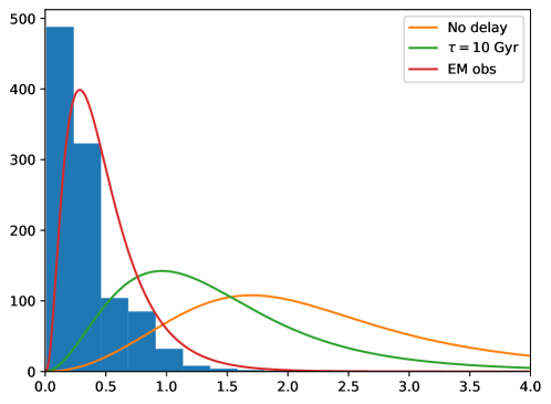
Figure 1: Histogram of redshift distribution of the 1048 supernovae used in Scolnic:2017caz to measure the luminosity distance relationship (blue) compared with merger event distribution for different source distributions. Third-generation observatories can detect binary neutron stars up to $z\simeq 2$. Distributions have been normalised to have an equal number of events, i.e. 1048.

We assume that redshifts can be determined with negligible uncertainty in the presence of an electromagnetic counterpart (see DelPozzo:2011yh ; Abbott:2019yzh for measuring the Hubble constant $H_{0}$ without electromagnetic counterpart) and the uncertainty in $d_{L}$ has usually two main contributions: an instrumental one intrinsic to GW observatories here denoted as $(\Delta d_{L})_{inst}$ Zhao:2010sz , and another one $(\Delta d_{L})_{lens}$ due to lensing, see e.g. Bonvin:2005ps ; Hirata:2010ba , see also Bonvin:2016qxr for an additional source of bias in intrinsic parameters measure by GW detections). Adding the sub-leading source of error due to peculiar velocities Gordon:2007zw one has:

$$\frac{\Delta d_{L}(z)}{d_{L}(z)}=\left[\left(\frac{\Delta d_{L}(z)}{d_{L}(z)}\right)_{inst}^{2}+\left(\frac{\Delta d_{L}(z)}{d_{L}(z)}\right)_{lens}^{2}+\left(\frac{\Delta d_{L}(z)}{d_{L}(z)}\right)_{pec}^{2}\right]^{1/2}\,,$$ (14)

with

$$\begin{array}[]{rcl}\displaystyle\left(\frac{\Delta d_{L}(z)}{d_{L}(z)}\right)_{inst}&\approx&\displaystyle 0.1449z-0.0118z^{2}+0.0012z^{3}\,,\\ \displaystyle\left(\frac{\Delta d_{L}(z)}{d_{L}(z)}\right)_{lens}&\approx&\displaystyle 0.066\left[4\left(1-(1+z)^{-1/4}\right)\right]^{1.8}\,,\\ \displaystyle\left(\frac{\Delta d_{L}(z)}{d_{L}(z)}\right)_{pec}&\approx&\displaystyle\left|1-\frac{\left(1+z\right)^{2}}{H(z)d_{L}(z)}\right|\frac{\sigma_{v}}{c}\,,\qquad\sigma_{v}=331{\rm km/sec}\,,\end{array}$$ (15)

which are shown in fig. 2 (with $c$ being the speed of light).

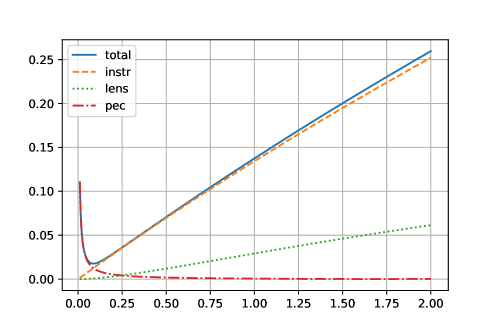
Figure 2: Uncertainty budget in the determination of the luminosity distance by third-generation detector like ET Zhao:2010sz ; Hirata:2010ba ; Gordon:2007zw as a function of redshift, see eq. (15). Instrumental effects give the leading uncertainty for all redshift of interest.

Note that a reduction in luminosity distance error may come from combining more than one third-generation detector, as shown in Vitale:2018nif , leading to an error lower than 10% in the red-shift range of our interest. This is why we also consider in the next section the case in which the distance error is reduced to the lensing limit, which roughly amounts to 20% of the total error budget displayed in fig. 2.. The last source of error in redshift determination in eq. (14,15), the one due to peculiar velocities, is important only for $z\lesssim 0.1$, where a negligible number of detections are present, see fig. 4, hence it will be neglected in this work.

III Results

This section reports the result obtained by simulating 1,000 detections of electromagnetically bright coalescing binaries up to redshift $z=2$ with realistic distributions of events and comparing phenomenological models for late time cosmological acceleration within the Bayesian model selection framework. We use two different laws for relating the standard siren luminosity distance and redshift of the data:

1. the standard $\Lambda$CDM which we also use at recovery, with parameters $\Omega_{m}=0.3111$, $H_{0}=67.66\rm{km/s/Mpc}$, $\Omega_{\Lambda}=1-\Omega_{m}$ taken from Aghanim:2018eyx ,

2. the non-local massive gravity (massG) model Belgacem:2017cqo , useful as a testing ground for different models at recovery, none of which include the massG model used in this second set of injections. Note that since the background evolution in this model is different than any of the $\Lambda$CDM and $w$CDM, the best-fit background parameter value are slightly different than in the previous case: $\Omega_{m}=0.2989$, $H_{0}=69.49\rm{km/s/Mpc}$ Dirian:2017pwp .

Each of the two sets of simulated data ($\Lambda$CDM and massG) is produced for three different distributions of merger events:

1. one following the star formation rate proposed in Madau:2014bja , orange solid line in fig. 1,

2. the second allowing a Poisson distributed delay between star formation and binary merger with average delay $\tau=10$ Gyr, green solid line in fig. 1,

3. the last one following the realistic observed rate given in eq. (13), referred to as EMobs, red solid line in fig. 1,

resulting in six different sets of injections. Fig. 3 displays explicitly one of the six types of injections we use, and in fig. 4 the cumulative distributions of the 1,000 injections are reported for the six cases, showing little difference between the $\Lambda$CDM and $massG$ case, but a notable difference among the three underlying cosmological distributions of mergers.

We use these six type of simulated data for comparing $\Lambda$CDM versus $w$CDM and $\Lambda$CDM versus $w_{0}w_{a}$CDM, with the results for model comparisons displayed respectively in figs. 5,6 for $\Lambda$CDM injections, and in figs. 7,8 for $massG$ injections. The 1,000 simulated detections are divided in 100 catalogs of 10 detections each, for each graph 50 different injections realizations have been performed, shady regions representing 1-$\sigma$ level around the thick line showing the average value.

Results are obtained via the Nestle implementation Mukherjee:2005wg of the nested sampling algorithm Skilling:2006gxv using 200 live points. Priors for all have been chosen flat in the intervals: $H_{0}:[60,80]$ km/s/Mpc, $\Omega_{m}:[0.2,0.4]$, $w_{0}:[-2,0]$, $w_{a}:[-1,1]$.

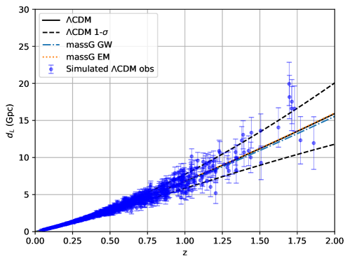
Figure 3: One thousand events simulated according to the EMobs merger rate of eq. (13), with $1\sigma$ error band given by eq. (15) Zhao:2010sz ; Tamanini:2016zlh . For reference, the luminosity distance versus redshift curve for $\Lambda$CDM and massG models are also shown, for best fit parameters respectively given in Aghanim:2018eyx and Dirian:2017pwp .

Figure 4: Cumulative distribution of injections for $\Lambda$CDM and the massG modelBelgacem:2017cqo as a function of redshift for the cases, from bottom to top, of no delay between star formation eq. (10) and binary mergers, $\tau=10$Gyr Poissonianly-distributed stochastic delay between star formation and mergers eq. (12), and EM-observed distribution eq. (13).

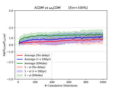
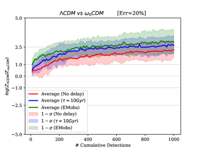
Figure 5: Evidence for $\Lambda$CDM versus $w$CDM model with 1,000 events, simulated according to the $\Lambda$CDM model with standard uncertainty in the luminosity distance given by eq. (15) (left) and uncertainty reduced to $20\%$ (right), with merger rate equal to star formation rate, convolved with a Poisson-distributed $\tau=10$ Gyr delay as in eq. (12) between formation and merger, and according to EMobs distribution eq. (13). From 50 different injection realizations the shady regions corresponds to 1-$\sigma$ level around the thick line showing the average value. Weak, moderate and strong evidence reference lines are also displayed for $\ln Z_{1}/Z_{2}=\pm 1,\pm 2.5,\pm 5$) according to Jeffreys’ scale.

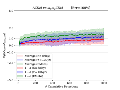
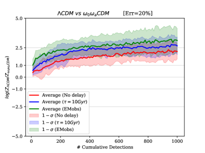
Figure 6: Analog to fig. 5 for $\Lambda$CDM versus $w_{0}w_{a}$CDM model: simulated 1,000 events following $\Lambda$CDM model, standard $d_{L}$ uncertainty (left) and reduced uncertainty, $20\%$ of eq. (15) (right), with merger rate equal to star formation rate, convolved with a Poisson-distributed $\tau=10$ Gyr delay as in eq. (12) between formation and merger, and according to EMobs distribution eq. (13). From 50 different injection realizations the shady regions corresponds to 1-$\sigma$ level around the thick line showing the average value.

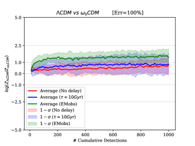
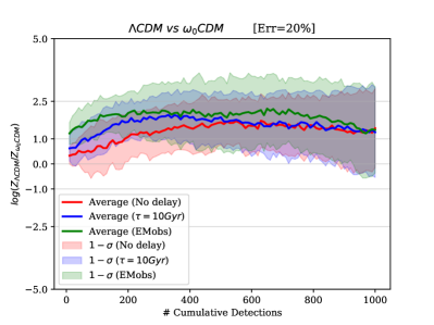
Figure 7: Analog to fig. 5 for simulated data following the massG model Belgacem:2017cqo : evidence for $\Lambda$CDM versus $w$CDM models with 1,000 events, standard $d_{L}$ uncertainty eq. (15) (left) and uncertainty reduced to 20% (right), with merger rate equal to star formation rate, convolved with a Poisson-distributed $\tau=10$ Gyr delay as in eq. (12) between formation and merger, and according to EMobs distribution eq. (13). From 50 different injection realizations the shady regions corresponds to 1-$\sigma$ level around the thick line showing the average value. Moderate and strong evidence reference lines ($\ln Z_{1}/Z_{2}=\pm 2.5,\pm 5$ according to Jeffreys’ scale) are also shown for reference.

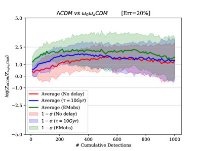
Figure 8: Same as in fig. 5 for simulated data following the massG modelBelgacem:2017cqo : evidence for $\Lambda$CDM versus $w_{0}w_{a}$CDM models with 1,000 events. Standard $d_{L}$ uncertainty (left) and reduced uncertainty (right), with merger rate equal to star formation rate, convolved with a Poisson-distributed $\tau=10$ Gyr delay as in eq. (12) between formation and merger, and according to EMobs distribution eq. (13). From 50 different injection realizations the shady regions corresponds to 1-$\sigma$ level around the thick line showing the average value.

Fig. 5 shows the evidence comparison for $\Lambda$CDM versus $w$CDM, with simulated data following the $\Lambda$CDM model and taken from a distribution of merger events following the star formation rate of eq. (10) Madau:2014bja , the same star formation rate convoluted with a delay with a Poisson distribution with average $\tau=10$Gyr, and EMobs rate (13), each of the three cases with luminosity distance uncertainties as in eq. (14) and with uncertainties reduced to 20% that value.

All evidence ratios correctly favor $\Lambda$CDM vs. $w$CDM, as expected since injections follow the $\Lambda$CDM model, and reducing observational uncertainty strengthens the discriminating power of the Bayes model selection test, with the logarithm of evidence ratio approaching the weak to moderate evidence line $\ln Z_{\Lambda CDM}/Z_{wCDM}=2.5$, see Jeffreys’ scale jeffreys ; Trotta:2008qt , for the reduced error cases. Note also that having the detections at lower redshifts, where the luminosity distance measure error is smaller, gives more discriminating power.

Analogously in fig.6 $\Lambda$CDM is ranked against $w_{0}w_{a}$CDM, i.e. against a model with two extra parameters that contains $\Lambda$CDM for $w_{0}=-1$, $w_{a}=0$ for two sets of $d_{L}$ uncertainties and three sets of signal distributions as above, again with the result of the $\Lambda$CDM model being favored. Again reducing the measurement errors and taking the detections at relative lower redshifts have the effect of increasing the discriminating power of the data, showing that event distribution with redshift also plays an important role.

In figs. 7,8 the same exercise is replayed, with the difference of using injections belonging to the massG model Belgacem:2017cqo , hence not being described by any of the nested models used for recovery, which are again $\Lambda$CDM and $w$CDM in fig. 7, and $\Lambda$CDM and $w_{0}w_{a}$CDM in 8. In this case, in which none of the recovery models coincide with the one used for injections, irrespectively of the assumptions on the error on the luminosity distance and event distribution, the outcome of evidence comparison is inconclusive, and specific realizations can give logarithm of Bayes’ factor ratios with both signs. This indicates that future inconclusive results in comparing models may be due to the lack of appropriate parameterization to describe data.

B reports the comparison between $\Lambda$CDM and massG models over simulations based on the massG model.

IV Conclusions

Motivated by the advent of gravitational wave astronomy and by the first measure of the Hubble constant via standard sirens, we have performed a numerical exercise simulating future measurements of the luminosity distance versus redshift relationship via combined detections of gravitational and electromagnetic waves to test their power in discriminating among cosmological models of late time acceleration.

There are two main conclusions that we can draw from our simulations. The first is that the error in luminosity distance as estimated in eq. (14) should be decreased to enable model comparison with future gravitational wave detectors. This should be possible by correlating the output of several observatories Vitale:2016icu : in particular, for the case of the Einstein Telescope combining several detectors can lead to substantial improvement (a factor of few) in the luminosity distance error with respect to a single detector. However even reducing at maximum the detector intrinsic uncertainty, the lensing limit becomes a limit factor for the measure of the luminosity distance, as also underlined in Belgacem:2019tbw .

The second main conclusions are that the intrinsic event distribution also plays an important role: distributing events at smaller distances concentrate events where observational error are smaller and hence convey more information, even if different models tend all to reproduce the same dynamics for small redshifts ($z\lesssim 1$) and disagree more at larger redshifts ($z\gtrsim 2$).

Note that the expected rate of standard siren accompanied by electromagnetic detections is subject to large uncertainties, but a reasonably optimistic expectation corresponds to few dozens of events per year, thus requiring several years to accumulate $O(10^{3})$ detections Belgacem:2019tbw .

Finally, we underline that in case the dynamics underlying observations are only approximately described by models used to analyze data, different models may have comparable performance on data, leaving open the search for a better model able to catch the right physics conveyed by the observations.

We also note that while cosmological model discrimination at low redshift may be hard, future observations of gravitational standard sirens by LISA in conjunction with Quasar electromagnetic detections at $z\gtrsim 3$ may be powerful for luminosity distance typical precision of the order of 10%, as demonstrated in Speri:2020hwc , where $\Lambda$CDM can be discriminated against the alternative model originally proposed in Risaliti:2018reu already with a handful of detections.
On the other hand future joint analysis of electromagnetic and gravitational observations are expected to reach sub-percent precision in $\Lambda$CDM deviation parameters $w_{0,a}$, helping the quest for a more fundamental cosmological model.

Appendix A Comparison of nested models

As additional material, we report in fig. 9 the comparison of the logarithm of evidence ratios between nested models $\Lambda$CDM and $w$CDM obtained numerically after averaging over 50 sets of 1,000 $\Lambda$CDM injections each, and the theoretical analytic estimate in eq. (9) as a function on $\Sigma$, the width of the prior on the extra variable. We remind the reader that in our numerical analysis the prior over $w_{0}$ is flat between in the interval $[-2,0]$, thus finding consistency between our analysis and the theoretical prediction eq. (9).

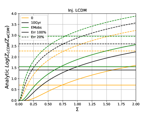
Figure 9: Comparison between analytic estimate of log Bayes ratio for $\Lambda$CDM vs. $w$CDM model from eq. (9) as a function of $w_{0}$ prior width $\Sigma$ compared with the values obtained numerically (horizontal lines) in the simulation described in this work, averaging over 50 realisations of 1,000 injections.

Appendix B Comparison of $\Lambda$CDM and massive gravity models

As a consistency check in fig. 10 we report the logarithm of evidence ratios between $\Lambda$CDM and massG models for massG injections, which indicates a better discriminating power for simulations with reduced errors and distributed at relatively lower redshift.

In Belgacem:2018lbp a comparison between the massG and the $\Lambda$CDM model was performed by comparing respective $\chi^{2}$ values at best fit, whereas we report evidence ratios (which is roughly the likelihood integrated over search parameters with appropriate priors) which are described in sec. II. Our results are broadly in agreement with those in Belgacem:2018lbp , which we could reproduce computing $\chi^{2}$ values (not reported here) instead of evidences.

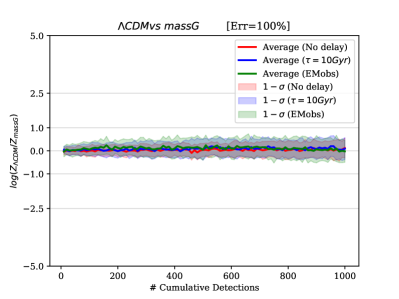
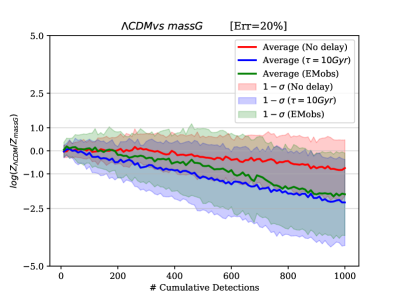
Figure 10: Evidence for $\Lambda$CDM versus massG models with $1000$ events simulated according to the massG model with standard uncertainty in the luminosity distance given by eq. (15) (left) and uncertainty reduced to $20\%$ (right), with merger rate equal to star formation rate, convolved with a Poisson-distributed $\tau=10$ Gyr delay as in eq. (12) between formation and merger and according to eq. (13). From 50 different injections realisations the shady regions corresponds to 1-$\sigma$ level around the thick line showing the average value.

References

- (1) B. Abbott, et al., GW170817: Observation of Gravitational Waves from a Binary Neutron Star Inspiral, Phys. Rev. Lett. 119 (16) (2017) 161101. arXiv:1710.05832, doi:10.1103/PhysRevLett.119.161101.
- (2) B. P. Abbott, et al., Multi-messenger Observations of a Binary Neutron Star Merger, Astrophys. J. 848 (2) (2017) L12. arXiv:1710.05833, doi:10.3847/2041-8213/aa91c9.
- (3) B. F. Schutz, Determining the Hubble Constant from Gravitational Wave Observations, Nature 323 (1986) 310–311. doi:10.1038/323310a0.
- (4) D. E. Holz, S. A. Hughes, Using gravitational-wave standard sirens, Astrophys. J. 629 (2005) 15–22. arXiv:astro-ph/0504616, doi:10.1086/431341.
- (5) A. G. Riess, et al., A 2.4% Determination of the Local Value of the Hubble Constant, Astrophys. J. 826 (1) (2016) 56. arXiv:1604.01424, doi:10.3847/0004-637X/826/1/56.
- (6) C. Messenger, J. Read, Measuring a cosmological distance-redshift relationship using only gravitational wave observations of binary neutron star coalescences, Phys. Rev. Lett. 108 (2012) 091101. arXiv:1107.5725, doi:10.1103/PhysRevLett.108.091101.
- (7) W. Del Pozzo, Inference of the cosmological parameters from gravitational waves: application to second generation interferometers, Phys. Rev. D86 (2012) 043011. arXiv:1108.1317, doi:10.1103/PhysRevD.86.043011.
- (8) M. Punturo, et al., The Einstein Telescope: A third-generation gravitational wave observatory, Class. Quant. Grav. 27 (2010) 194002. doi:10.1088/0264-9381/27/19/194002.
- (9) B. P. Abbott, et al., Exploring the Sensitivity of Next Generation Gravitational Wave Detectors, Class. Quant. Grav. 34 (4) (2017) 044001. arXiv:1607.08697, doi:10.1088/1361-6382/aa51f4.
- (10) G. M. Harry, Advanced LIGO: The next generation of gravitational wave detectors, Class. Quant. Grav. 27 (2010) 084006. doi:10.1088/0264-9381/27/8/084006.
- (11) F. Acernese, et al., Advanced Virgo: a second-generation interferometric gravitational wave detector, Class. Quant. Grav. 32 (2) (2015) 024001. arXiv:1408.3978, doi:10.1088/0264-9381/32/2/024001.
- (12) E. Belgacem, Y. Dirian, S. Foffa, E. J. Howell, M. Maggiore, T. Regimbau, Cosmology and dark energy from joint gravitational wave-GRB observations, JCAP 1908 (2019) 015. arXiv:1907.01487, doi:10.1088/1475-7516/2019/08/015.
- (13) A. G. Riess, S. Casertano, W. Yuan, L. Macri, J. Anderson, J. W. MacKenty, J. B. Bowers, K. I. Clubb, A. V. Filippenko, D. O. Jones, B. E. Tucker, New parallaxes of galactic cepheids from spatially scanning the hubble space telescope: Implications for the hubble constant, Astrophys. J. 136 (2018) 855. arXiv:1801.01120.
- (14) N. Aghanim, et al., Planck 2018 results. VI. Cosmological parameters, Astron. Astrophys. 641 (2020) A6. arXiv:1807.06209, doi:10.1051/0004-6361/201833910.
- (15) S. Birrer, et al., H0LiCOW - IX. Cosmographic analysis of the doubly imaged quasar SDSS 1206+4332 and a new measurement of the Hubble constant, Mon. Not. Roy. Astron. Soc. 484 (2019) 4726. arXiv:1809.01274, doi:10.1093/mnras/stz200.
-
(16)
Khetan, Nandita, Izzo, Luca, Branchesi, Marica, Wojtak, Radoslaw,
Cantiello, Michele, Murugeshan, Chandrashekar, Agnello, Adriano,
Cappellaro, Enrico, Della Valle, Massimo, Gall, Christa, Hjorth,
Jens, Benetti, Stefano, Brocato, Enzo, Burke, Jamison, Hiramatsu,
Daichi, Howell, D. Andrew, Tomasella, Lina, Valenti, Stefano,
A new measurement of the
hubble constant using type ia supernovae calibrated with surface brightness
fluctuations, A&A 647 (2021) A72.
doi:10.1051/0004-6361/202039196.
URL https://doi.org/10.1051/0004-6361/202039196 - (17) L. Verde, T. Treu, A. G. Riess, Tensions between the Early and the Late Universe, Nature Astron. 3 (2019) 891. arXiv:1907.10625, doi:10.1038/s41550-019-0902-0.
- (18) N. Dalal, D. E. Holz, S. A. Hughes, B. Jain, Short grb and binary black hole standard sirens as a probe of dark energy, Phys. Rev. D74 (2006) 063006. arXiv:astro-ph/0601275, doi:10.1103/PhysRevD.74.063006.
- (19) B. S. Sathyaprakash, B. F. Schutz, C. Van Den Broeck, Cosmography with the Einstein Telescope, Class. Quant. Grav. 27 (2010) 215006. arXiv:0906.4151, doi:10.1088/0264-9381/27/21/215006.
- (20) R.-G. Cai, T. Yang, Estimating cosmological parameters by the simulated data of gravitational waves from the Einstein Telescope, Phys. Rev. D95 (4) (2017) 044024. arXiv:1608.08008, doi:10.1103/PhysRevD.95.044024.
- (21) X.-N. Zhang, L.-F. Wang, J.-F. Zhang, X. Zhang, Improving cosmological parameter estimation with the future gravitational-wave standard siren observation from the Einstein Telescope, Phys. Rev. D99 (6) (2019) 063510. arXiv:1804.08379, doi:10.1103/PhysRevD.99.063510.
- (22) H.-Y. Chen, M. Fishbach, D. E. Holz, A two per cent Hubble constant measurement from standard sirens within five years, Nature 562 (7728) (2018) 545–547. arXiv:1712.06531, doi:10.1038/s41586-018-0606-0.
- (23) S. Camera, A. Nishizawa, Beyond Concordance Cosmology with Magnification of Gravitational-Wave Standard Sirens, Phys. Rev. Lett. 110 (15) (2013) 151103. arXiv:1303.5446, doi:10.1103/PhysRevLett.110.151103.
- (24) A. Nishizawa, Generalized framework for testing gravity with gravitational-wave propagation. I. Formulation, Phys. Rev. D97 (10) (2018) 104037. arXiv:1710.04825, doi:10.1103/PhysRevD.97.104037.
- (25) S. Arai, A. Nishizawa, Generalized framework for testing gravity with gravitational-wave propagation. II. Constraints on Horndeski theory, Phys. Rev. D97 (10) (2018) 104038. arXiv:1711.03776, doi:10.1103/PhysRevD.97.104038.
- (26) A. Nishizawa, S. Arai, Generalized framework for testing gravity with gravitational-wave propagation. III. Future prospect, Phys. Rev. D99 (10) (2019) 104038. arXiv:1901.08249, doi:10.1103/PhysRevD.99.104038.
- (27) R.-G. Cai, N. Tamanini, T. Yang, Reconstructing the dark sector interaction with LISA, JCAP 1705 (05) (2017) 031. arXiv:1703.07323, doi:10.1088/1475-7516/2017/05/031.
- (28) T. M. C. Abbott, et al., First Cosmology Results using Type Ia Supernovae from the Dark Energy Survey: Constraints on Cosmological Parameters, Astrophys. J. 872 (2) (2019) L30. arXiv:1811.02374, doi:10.3847/2041-8213/ab04fa.
- (29) S. R. Taylor, J. R. Gair, Cosmology with the lights off: standard sirens in the Einstein Telescope era, Phys. Rev. D86 (2012) 023502. arXiv:1204.6739, doi:10.1103/PhysRevD.86.023502.
- (30) A. Blanchard, et al., Euclid preparation: VII. Forecast validation for Euclid cosmological probes, Astron. Astrophys. 642 (2020) A191. arXiv:1910.09273, doi:10.1051/0004-6361/202038071.
- (31) M. Chevallier, D. Polarski, Accelerating universes with scaling dark matter, Int. J. Mod. Phys. D10 (2001) 213–224. arXiv:gr-qc/0009008, doi:10.1142/S0218271801000822.
- (32) E. V. Linder, Exploring the expansion history of the universe, Phys. Rev. Lett. 90 (2003) 091301. arXiv:astro-ph/0208512, doi:10.1103/PhysRevLett.90.091301.
- (33) E. Belgacem, Y. Dirian, S. Foffa, M. Maggiore, Nonlocal gravity. Conceptual aspects and cosmological predictions, JCAP 1803 (03) (2018) 002. arXiv:1712.07066, doi:10.1088/1475-7516/2018/03/002.
- (34) E. Belgacem, Y. Dirian, S. Foffa, M. Maggiore, Modified gravitational-wave propagation and standard sirens, Phys. Rev. D98 (2) (2018) 023510. arXiv:1805.08731, doi:10.1103/PhysRevD.98.023510.
- (35) R. Trotta, Bayes in the sky: Bayesian inference and model selection in cosmology, Contemp. Phys. 49 (2008) 71–104. arXiv:0803.4089, doi:10.1080/00107510802066753.
- (36) W. Zhao, C. Van Den Broeck, D. Baskaran, T. G. F. Li, Determination of Dark Energy by the Einstein Telescope: Comparing with CMB, BAO and SNIa Observations, Phys. Rev. D83 (2011) 023005. arXiv:1009.0206, doi:10.1103/PhysRevD.83.023005.
- (37) S. Vitale, M. Evans, Parameter estimation for binary black holes with networks of third generation gravitational-wave detectors, Phys. Rev. D95 (6) (2017) 064052. arXiv:1610.06917, doi:10.1103/PhysRevD.95.064052.
- (38) B. S. Sathyaprakash, et al., Multimessenger Universe with Gravitational Waves from BinariesarXiv:1903.09277.
- (39) P. Madau, M. Dickinson, Cosmic Star Formation History, Ann. Rev. Astron. Astrophys. 52 (2014) 415–486. arXiv:1403.0007, doi:10.1146/annurev-astro-081811-125615.
- (40) S. Vitale, W. M. Farr, K. Ng, C. L. Rodriguez, Measuring the star formation rate with gravitational waves from binary black holes, Astrophys. J. Lett. 886 (1) (2019) L1. arXiv:1808.00901, doi:10.3847/2041-8213/ab50c0.
- (41) M. Safarzadeh, E. Berger, K. K. Y. Ng, H.-Y. Chen, S. Vitale, C. Whittle, E. Scannapieco, Measuring the delay time distribution of binary neutron stars. II. Using the redshift distribution from third-generation gravitational wave detectors network, Astrophys. J. 878 (1) (2019) L13. arXiv:1904.10976, doi:10.3847/2041-8213/ab22be.
- (42) D. M. Scolnic, et al., The Complete Light-curve Sample of Spectroscopically Confirmed SNe Ia from Pan-STARRS1 and Cosmological Constraints from the Combined Pantheon Sample, Astrophys. J. 859 (2) (2018) 101. arXiv:1710.00845, doi:10.3847/1538-4357/aab9bb.
- (43) D. Meacher, M. Coughlin, S. Morris, T. Regimbau, N. Christensen, S. Kandhasamy, V. Mandic, J. D. Romano, E. Thrane, Mock data and science challenge for detecting an astrophysical stochastic gravitational-wave background with Advanced LIGO and Advanced Virgo, Phys. Rev. D92 (6) (2015) 063002. arXiv:1506.06744, doi:10.1103/PhysRevD.92.063002.
- (44) B. P. Abbott, et al., A Gravitational-wave Measurement of the Hubble Constant Following the Second Observing Run of Advanced LIGO and Virgo, Astrophys. J. 909 (2) (2021) 218. arXiv:1908.06060, doi:10.3847/1538-4357/abdcb7.
- (45) C. Bonvin, R. Durrer, M. A. Gasparini, Fluctuations of the luminosity distance, Phys. Rev. D73 (2006) 023523, [Erratum: Phys. Rev.D85,029901(2012)]. arXiv:astro-ph/0511183, doi:10.1103/PhysRevD.85.029901,10.1103/PhysRevD.73.023523.
- (46) C. M. Hirata, D. E. Holz, C. Cutler, Reducing the weak lensing noise for the gravitational wave Hubble diagram using the non-Gaussianity of the magnification distribution, Phys. Rev. D81 (2010) 124046. arXiv:1004.3988, doi:10.1103/PhysRevD.81.124046.
- (47) C. Bonvin, C. Caprini, R. Sturani, N. Tamanini, Effect of matter structure on the gravitational waveform, Phys. Rev. D95 (4) (2017) 044029. arXiv:1609.08093, doi:10.1103/PhysRevD.95.044029.
- (48) C. Gordon, K. Land, A. Slosar, Cosmological Constraints from Type Ia Supernovae Peculiar Velocity Measurements, Phys. Rev. Lett. 99 (2007) 081301. arXiv:0705.1718, doi:10.1103/PhysRevLett.99.081301.
- (49) S. Vitale, C. Whittle, Characterization of binary black holes by heterogeneous gravitational-wave networks, Phys. Rev. D98 (2) (2018) 024029. arXiv:1804.07866, doi:10.1103/PhysRevD.98.024029.
- (50) N. Tamanini, C. Caprini, E. Barausse, A. Sesana, A. Klein, A. Petiteau, Science with the space-based interferometer eLISA. III: Probing the expansion of the Universe using gravitational wave standard sirens, JCAP 1604 (04) (2016) 002. arXiv:1601.07112, doi:10.1088/1475-7516/2016/04/002.
- (51) Y. Dirian, Changing the Bayesian prior: Absolute neutrino mass constraints in nonlocal gravity, Phys. Rev. D96 (8) (2017) 083513. arXiv:1704.04075, doi:10.1103/PhysRevD.96.083513.
- (52) P. Mukherjee, D. Parkinson, A. R. Liddle, A nested sampling algorithm for cosmological model selection, Astrophys. J. 638 (2006) L51–L54. arXiv:astro-ph/0508461, doi:10.1086/501068.
- (53) J. Skilling, Nested sampling for general Bayesian computation, Bayesian Analysis 1 (4) (2006) 833–859. doi:10.1214/06-BA127.
- (54) H. Jeffreys, Theory of probability, Clarendon Press, Oxford, 1961, 3rd edn 1998.
- (55) L. Speri, N. Tamanini, R. R. Caldwell, J. R. Gair, B. Wang, Testing the Quasar Hubble Diagram with LISA Standard SirensarXiv:2010.09049.
- (56) G. Risaliti, E. Lusso, Cosmological constraints from the Hubble diagram of quasars at high redshifts, Nature Astron. 3 (3) (2019) 272–277. arXiv:1811.02590, doi:10.1038/s41550-018-0657-z.