Optimal operator preconditioning for pseudodifferential boundary problems

Abstract

We propose an operator preconditioner for general elliptic pseudodifferential equations in a domain $\Omega$, where $\Omega$ is either in $\mathbb{R}^{n}$ or in a Riemannian manifold. For linear systems of equations arising from low-order Galerkin discretizations, we obtain condition numbers that are independent of the mesh size and of the choice of bases for test and trial functions. The basic ingredient is a classical formula by Boggio for the fractional Laplacian, which is extended analytically. In the special case of the weakly and hypersingular operators on a line segment or a screen, our approach gives a unified, independent proof for a series of recent results by Hiptmair, Jerez-Hanckes, Nédélec and Urzúa-Torres. We also study the increasing relevance of the regularity assumptions on the mesh with the order of the operator. Numerical examples validate our theoretical findings and illustrate the performance of the proposed preconditioner on quasi-uniform, graded and adaptively generated meshes.

1 Introduction

This article considers the Dirichlet problem for an elliptic pseudodifferential operator $A$ of order $2s$ in a bounded Lipschitz domain $\Omega$, where $\Omega$ is either a subset of $\mathbb{R}^{n}$, or, more generally, in a Riemannian manifold $\Gamma$:

$$\begin{cases}Au=f\qquad&\text{in }\Omega,\\ u=0\qquad&\text{in }\Gamma\setminus\overline{\Omega}.\end{cases}$$ (1)

Such pseudodifferential boundary problems are of interest in several applications. For instance, the integral fractional Laplacian $A=(-\Delta)^{s}$ and its variants $A=\$ $\mathrm{div}(c(x)\nabla^{2s-1}u)$ in a domain $\Omega\subset\mathbb{R}^{n}$ arise in the pricing of stock options (tankov, , Chapter 12), image processing go , continuum mechanics d , and in the movement of biological organisms egp ; egps or swarm robotic systems eg2 . By considering $\Omega\subset\Gamma$ (with $\Gamma$ a Riemannian manifold), one can also study the equations for the weakly singular ($A=\operatorname{\mathsf{V}}$) or hypersingular ($A=\operatorname{\mathsf{W}}$) operators arising from boundary integral formulations of the first kind for an elliptic boundary problem on curve segments or on open surfaces (ss, , Section 3.5.2). Another interesting example would be, in potential theory, where boundary problems of negative order arise for the Riesz potential (l, , Chapter 1, Section 3).

On the one hand, the bilinear form associated to $A$ is nonlocal, and its Galerkin discretization results in dense matrices. On the other hand, the condition number of the Galerkin matrices when using low-order piecewise polynomial basis function is of order $\mathcal{O}(h^{-2|s|})$, where $h$ is the size of the smallest cell of the mesh. Therefore, the solution of the resulting linear system via iterative solvers becomes prohibitively slow on fine meshes.

The preconditioning of pseudodifferential equations has been considered in different contexts. Classically, boundary element methods have been of interest, where multigrid and additive Schwarz methods am1 ; dirk ; ts , (ss, , Chapter 6), as well as operator preconditioners sw have been studied. A popular choice is operator preconditioning based on an elliptic pseudodifferential operator of the opposite order $-2s$, yet it leads to growing condition numbers when boundary conditions are not respected. Indeed, in the case $s=\frac{1}{2}$, the achieved condition number grows like $|\log(h)|^{n+1}$ for $n=1$ (ms, , Theorem 4.1) and $n=2$ (CHR02, , Proposition 1.3.5). We prove that the situation worsens for $|s|>\frac{1}{2}$, and the condition number may increase like $h^{1-2|s|}$, as we discuss in Section 5. Therefore, the “opposite order” strategy for $A$ in (1) could be far from optimal. This motivates the approach we pursue here, which incorporates the boundary conditions.

The aforementioned suboptimality was recently overcome for the weakly singular and hypersingular operators $\operatorname{\mathsf{V}}$ and $\operatorname{\mathsf{W}}$ on open $2d$ surfaces hju and curve segments hju0 , respectively. The proposed preconditioners were based on new exact formulas for the inverses of these operators on the flat disk hju1 and interval $[-1,1]$ jn . It is important to mention that, in this context, this article provides a novel and independent approach to the preconditioners used in hju1 ; hju : As discussed in Remark 2, by identifying $\Omega\subset\mathbb{R}^{n}$ with the flat screen $\Omega\times\{0\}\subset\mathbb{R}^{n+1}$, $\operatorname{\mathsf{W}}$ coincides with the fractional Laplacian $\frac{1}{2}(-\Delta)^{s}$ for $s=\frac{1}{2}$, while $\operatorname{\mathsf{V}}$ coincides with $\frac{1}{2}(-\Delta)^{s}$ for $s=-\frac{1}{2}$. Boggio’s classical formula (Equation (10) below) for the fractional Laplacian in the unit ball of $\mathbb{R}^{n}$, respectively its analytic extension to $s\in\mathbb{C}$, therefore recovers the exact formulas for $\operatorname{\mathsf{V}}^{-1}$ and $\operatorname{\mathsf{W}}^{-1}$ from hju1 ; jn as special cases. This connection between the fractional Laplacian and boundary integral equations was only known in $1D$ jn , and we extend it to arbitrary dimension. As a consequence, we obtain a unified and general preconditioning strategy for pseudodifferential problems, which includes $\operatorname{\mathsf{V}}$, $\operatorname{\mathsf{W}}$ and $(-\Delta)^{s}$.

Recently, the fractional Laplacian has attracted interest in itself. Multigrid preconditioners have been briefly mentioned in ag , while additive Schwarz preconditioners of BPX-type are currently being investigated bpxnochetto ; fmpp . Applied to this particular operator $A$, our results lead to the first operator preconditioner. This offers the advantage of benefiting from all the rigorous results of the operator preconditioning theory, including its applicability to non-uniformly refined meshes, while being easily implementable. Indeed, solutions to (1) feature edge singularities, analogous to those for the fractional Laplacian (g3, , Theorem 4). Therefore, when discretizing with low-order finite elements, one requires local refinement to recover optimal convergence rates. Hence, it becomes mandatory that preconditioners can deal with these non-uniform meshes.

Our main result for preconditioning can be found in Theorem 5.1; the proposed preconditioner $\mathbf{P}$ is optimal in the sense that the bound for the condition number neither depends on the mesh refinement, nor on the choice of bases for trial and test spaces.

We verify that the preconditioner may be used on shape regular algebraically graded meshes, which lead to quasi-optimal convergence rates for piecewise linear elements. We prove that the required mesh assumptions also hold for a natural class of adaptively refined meshes. By doing this, we show for the first time that operator preconditioning with standard low-order primal-dual finite element discretization does apply to these adaptive meshes. Our proof in fact shows the $H^{1}(\Omega)$-stability of the generalized (Petrov-Galerkin) $L^{2}(\Omega)$ projection on low-order finite element spaces, which may also have applications beyond preconditioning.

Outline of this article: Section 2 recalls basic notions of fractional Sobolev spaces. The fractional Laplacian and Boggio’s formula are discussed in Section 3. There we also explain how to use the latter to define a bilinear form associated to the solution operator in the ball. As special cases, we recover the recent solution formulas for the weakly and hypersingular operators $\operatorname{\mathsf{V}}$ and $\operatorname{\mathsf{W}}$. Section 4 introduces the pseudodifferential Dirichlet problem (1). Next, in Section 5, we recall the operator preconditioning theory and summarize discretization strategies under which Theorem 5.1 holds. In particular, Section 5.2 discusses the case of adaptively refined meshes. The article concludes with numerical experiments and their discussion in Section 6.

2 Sobolev Spaces

We recall some basic definitions and properties related to Sobolev spaces of non-integer order and to the fractional Laplacian. For further details we refer to ajs ; t ; fkv .

Let $\Omega\subset\mathbb{R}^{n}$ be a bounded Lipschitz domain, and for $s\in\mathbb{N}_{0}$, $H^{s}(\Omega)$ the Sobolev space of functions in $L^{2}(\Omega)$ whose distributional derivatives of order $s$ belong to $L^{2}(\Omega)$. For $s\in(0,\infty)$, we write $m=\lfloor s\rfloor$ and $\sigma=s-m$ and define the Sobolev space $H^{s}(\Omega)$ as

$$H^{s}(\Omega):=\{v\in H^{m}(\Omega):|\partial^{\alpha}v|_{H^{\sigma}(\Omega)}<\infty\ \ \forall|\alpha|=m\}\ .$$

Here $|\cdot|_{H^{\sigma}(\Omega)}$ is the Aronszajn-Slobodeckij seminorm

$$|v|_{H^{\sigma}(\Omega)}^{2}:=\iint_{\Omega\times\Omega}\frac{(v(x)-v(y))^{2}}{|x-y|^{n+2\sigma}}\mathop{}\!\mathrm{d}y\mathop{}\!\mathrm{d}x.$$

$H^{s}(\Omega)$ is a Hilbert space endowed with the norm

$$\|v\|_{H^{s}(\Omega)}^{2}:=\|v\|_{H^{m}(\Omega)}^{2}+\sum_{|\alpha|=m}|\partial^{\alpha}v|_{H^{\sigma}(\Omega)}^{2}.$$

Particularly relevant for this article are the Sobolev spaces (gs, , Chapter 4.1), (ml, , Chapter 3)

$${\widetilde{H}^{s}(\Omega):=\{v\in H^{s}(\mathbb{R}^{n}):\mathrm{supp}\;v\subset\overline{\Omega}\}}$$

of distributions whose extension by $0$ belongs to $H^{s}(\mathbb{R}^{n})$. In the literature, the spaces $\widetilde{H}^{s}(\Omega)$ are sometimes denoted by ${H}^{s}_{00}(\Omega)$.
We recall that when $\Omega$ is Lipschitz and $\frac{1}{2}\neq s\in(0,1)$, $\widetilde{H}^{s}(\Omega)$ coincides with the space $H^{s}_{0}(\Omega)$, which is the closure of $C^{\infty}_{0}(\Omega)$ with respect to the $H^{s}$-norm. Moreover, for $s\in(0,\frac{1}{2})$, $\widetilde{H}^{s}(\Omega)=H^{s}(\Omega)=H^{s}_{0}(\Omega)$. All three spaces differ when $s=\frac{1}{2}$.

For negative $s$ the Sobolev spaces are defined by duality, and in this article we denote the duality pairing between $\widetilde{H}^{s}(\Omega)$ and $H^{-s}(\Omega)$ by $\left\langle\cdot\,,\,\cdot\right\rangle_{\Omega}$. Using local coordinates, the definition of the Sobolev spaces extends to a bounded domain $\Omega$ of a Riemannian manifold $\Gamma$. For $|s|\leq 1$ the definition is independent of the choice of local coordinates, if $\Omega$ is Lipschitz (t, , Section 9).

3 The Fractional Laplacian

For $s\in(0,1)$, we define the fractional Laplacian of a function $u$ in the Schwartz space $\mathcal{S}(\mathbb{R}^{n})$ by

$$(-\Delta)^{s}u(x):=c_{n,s}\lim_{\varepsilon\to 0^{+}}\int_{\mathbb{R}^{n}\setminus{\color[rgb]{0,0,0}\operatorname{\overline{\mathcal{B}}}_{\varepsilon}(x)}}\frac{u(x)-u(y)}{|x-y|^{n+2s}}\mathop{}\!\mathrm{d}y\ ,$$ (2)

where $\mathcal{B}_{\varepsilon}(x)$ the $n$-dimensional ball of radius $\varepsilon>0$ centered at $x$. The normalization constant $c_{n,s}$ is defined in terms of $\mathsf{\Gamma}$ functions:

$$c_{n,s}:=\dfrac{2^{2s}s\mathsf{\Gamma}\left(\frac{n+2s}{2}\right)}{\pi^{\frac{n}{2}}\mathsf{\Gamma}\left(1-s\right)}.$$

For general $s>0$, we set $m:=\lfloor s\rfloor$, $\sigma:=s-m$, and define $(-\Delta)^{s}u=(-\Delta)^{m}(-\Delta)^{\sigma}u$ for $u$ in the Schwartz space.

Equivalently, the fractional Laplacian may be defined in terms of the Fourier transform on $\mathbb{R}^{n}$ as

$$\mathcal{F}((-\Delta)^{s}u)=|\xi|^{2s}\mathcal{F}u,$$ (3)

see for example (classicalbook, , Equation 25.2). For $s>0$ this formula extends $(-\Delta)^{s}$ to an unbounded operator on $L^{2}(\mathbb{R}^{n})$, as well as to an operator on the space of tempered distributions $\mathcal{S}^{\prime}(\mathbb{R}^{n})$.

To continue the definition of $(-\Delta)^{s}$ to complex values of $s$, recall that the homogeneous function $0\neq\xi\mapsto|\xi|^{2s}$ admits an extension to a (tempered) homogeneous distribution on $\operatorname{\mathbb{R}}^{n}$ for $s\in\mathbb{C}\setminus\mathcal{P}$ (classicalbook, , Equation 25.19) , with

$$\mathcal{P}:=\{m\in\frac{1}{2}\mathbb{Z}:m\leq-\frac{n}{2}\}.$$ (4)

Formula (3) then defines $(-\Delta)^{s}$ for $s\in\mathbb{C}\setminus\mathcal{P}$. As $|\xi|^{2s}$ extends to a meromorphic function of $s\in\mathbb{C}$ with values in the space of tempered distributions, in the sense of gro , so does $(-\Delta)^{s}=\mathcal{F}^{-1}\circ|\xi|^{2s}\circ\mathcal{F}$ as a meromorphic family in the space of operators from $\mathcal{S}(\mathbb{R}^{n})$ to $\mathcal{S}^{\prime}(\mathbb{R}^{n})$. We refer to (classicalbook, , Section 25) for details, as well as for the fact that $(-\Delta)^{s}$ admits a holomorphic continuation to $s=m\in\mathcal{P}$ on the subspace

$$\Phi_{m}:=\left\{u\in\mathcal{S}(\mathbb{R}^{n}):\forall\alpha\in\mathbb{N}^{n}_{0}\ \text{ with }\ |\alpha|\leq-2m-n:\langle x^{\alpha},u\rangle_{\mathbb{R}^{n}}=0\right\}\ .$$ (5)

For a careful investigation when $s=-\frac{n}{2}$, where $\Phi_{m}$ consists of functions of mean $0$, see also (stinga, , Section 3).

Formula (3) finally shows that $(-\Delta)^{s}$ is an operator of order $2\mathrm{Re}(s)$ and that for $s=1$ one recovers the ordinary Laplace operator. For a bounded domain $\Omega\subset\operatorname{\mathbb{R}}^{n}$, the former can be stated as: there holds the continuity $(-\Delta)^{s}:\widetilde{H}^{s}(\Omega)\to H^{-s}(\Omega)$ for $s\in\mathbb{R}$.

3.1 Dirichlet problem for the fractional Laplacian

In this article the homogeneous Dirichlet problem for the fractional Laplacian plays a special role as an “auxiliary problem”, which will help us construct preconditioners for (1).

For a bounded Lipschitz domain $\Omega\subset\mathbb{R}^{n}$ and $f\in L^{2}(\Omega)$, it is formally given by:

$$\begin{cases}(-\Delta)^{s}u=f\qquad&\text{in }\Omega,\\ u=0\qquad&\text{in }\mathbb{R}^{n}\setminus\overline{\Omega}.\end{cases}$$ (6)

For $s\in(0,1)$, its variational formulation is expressed in terms of the bilinear form ${\color[rgb]{0,0,0}\mathsf{c}}$ on $\widetilde{H}^{s}(\Omega)$,

$${\mathsf{c}}(u,v):=\frac{c_{n,s}}{2}\iint_{D}\frac{(u(x)-u(y))(v(x)-v(y))}{|x-y|^{n+2s}}\mathop{}\!\mathrm{d}y\mathop{}\!\mathrm{d}x\ ,$$ (7)

where $D:=(\mathbb{R}^{n}\times\Omega)\cup(\Omega\times\mathbb{R}^{n}){=(\mathbb{R}^{n}\times\mathbb{R}^{n})\setminus(\Omega^{c}\times\Omega^{c})}$. Similar formulas for $s>1$ may be found in (ajs, , Section 1.1).

Note that formally

$${\color[rgb]{0,0,0}\mathsf{c}}(u,v)=\langle(-\Delta)^{s}u,v\rangle_{{\color[rgb]{0,0,0}\mathbb{R}^{n}}}-{\color[rgb]{0,0,0}\frac{c_{n,s}}{2}}\iint_{\Omega^{c}\times\Omega^{c}}\frac{(u(x)-u(y))(v(x)-v(y))}{|x-y|^{n+2s}}\mathop{}\!\mathrm{d}y\mathop{}\!\mathrm{d}x,$$

when $u,v\in H^{s}(\mathbb{R}^{n})$, and the second term vanishes on $\widetilde{H}^{s}(\Omega)$. Here $\langle\cdot,\cdot\rangle_{\mathbb{R}^{n}}$ denotes the duality pairing from Section 2.

Using the Fourier definition (3), the bilinear form

$${\color[rgb]{0,0,0}\mathsf{c}}(u,v)=\langle(-\Delta)^{s}u,v\rangle_{{\color[rgb]{0,0,0}\mathbb{R}^{n}}}=\langle\mathcal{F}^{-1}(|\xi|^{2s}\mathcal{F}u),v\rangle_{{\color[rgb]{0,0,0}\mathbb{R}^{n}}}=\langle(\mathcal{F}^{-1}|\xi|^{2s})\ast u,v\rangle_{{\color[rgb]{0,0,0}\mathbb{R}^{n}}}$$ (8)

extends meromorphically to $s\in\mathbb{C}\setminus\mathcal{P}$. Here, $\ast$ denotes convolution. For $\mathrm{Re}(s)<0$ the inverse Fourier transform $\mathcal{F}^{-1}|\xi|^{2s}$ is locally integrable and the integrand is only weakly singular. Specifically, $\mathcal{F}^{-1}|\xi|^{2s}=c_{n,s}|x|^{-n-2s}$ for $\mathrm{Re}(s)<0$, $s\not\in\mathcal{P}$ ((classicalbook, , Equation 25.25)). For $s>0$ the relation between (8) and (7) is discussed in (classicalbook, , Section 25.4).

The weak formulation of (6) reads as follows:

Find $u\in\widetilde{H}^{s}(\Omega)$ such that

$${\color[rgb]{0,0,0}\mathsf{c}}(u,v)=\int_{\Omega}fv\mathrm{d}x,\qquad\forall v\in\widetilde{H}^{s}(\Omega).$$ (9)

Moreover, the bilinear form ${\color[rgb]{0,0,0}\mathsf{c}}$ is continuous and elliptic for $s>-\frac{n}{2}$ real: there exist $C_{{\color[rgb]{0,0,0}\mathsf{c}}},{\color[rgb]{0,0,0}\beta_{\mathsf{c}}}>0$ with

$${\color[rgb]{0,0,0}\mathsf{c}}(u,v)\leq C_{{\color[rgb]{0,0,0}\mathsf{c}}}\|u\|_{\widetilde{H}^{s}(\Omega)}\|v\|_{\widetilde{H}^{s}(\Omega)},\quad{\color[rgb]{0,0,0}\mathsf{c}}(u,u)\geq{\color[rgb]{0,0,0}\beta_{\mathsf{c}}}\|u\|_{\widetilde{H}^{s}(\Omega)}^{2}\ .$$

The ellipticity for $s>0$ follows by definition of the $\widetilde{H}^{s}(\Omega)$-norm, while the case $s\in(-\frac{n}{2},0)$ is a classical result in potential theory (l, , Page 358).

Therefore, by the Lax-Milgram theorem, the variational problem (9) admits a unique solution, and the solution operator $f\mapsto u$ extends to an isomorphism from $H^{-s}(\Omega)$ to $\widetilde{H}^{s}(\Omega)$ for all $s>-\frac{n}{2}$.

For $s\leq-\frac{n}{2}$ ellipticity requires additional assumptions, as in (5). Although we refrain from discussing these modifications in this article, it is worth pointing out that ellipticity is well known for $n=1$ and $s=-\frac{1}{2}$ in the case of the weakly singular integral operator from Remark 2 jn .

3.2 Solution operator in the unit ball

Let us write $\mathcal{B}_{1}$ for the unit ball $\mathcal{B}_{1}(0)\subset\mathbb{R}^{n}$. When $\Omega=\mathcal{B}_{1}$, explicit solution formulas are available. For $s>0$, the Green’s function in this case is given by

$$G_{s}(x,y):=k_{n,s}|x-y|^{2s-n}\int_{0}^{r(x,y)}\frac{t^{s-1}}{(t+1)^{n/2}}\operatorname{\mathrm{d}t},\qquad\forall x,y\in\mathbb{R}^{n},x\neq y.$$ (10)

Here $r(x,y):=\dfrac{(1-|x|^{2})_{+}(1-|y|^{2})_{+}}{|x-y|^{2}}$, $z_{+}:=\max\{z,0\}$ and $k_{n,s}:=\dfrac{2^{1-2s}}{|\partial\mathcal{B}_{1}|\mathsf{\Gamma}(s)^{2}}$.

For $s\in\mathbb{N}$, Formula (10) goes back to tb , while for $s\in(0,1)$ it has long been known in potential theory and Lévy processes (see e.g. (l, , Chapter 1, Section 3) and (riesz, , Chapter 5, Equation 3)). The extension to arbitrary order $s>0$ is more recent and may be found in ajs .

The following theorem from ajs shows that $G_{s}$ in formula (10) indeed defines the weakly singular integral kernel of the solution operator to (6) for $s>0$. More precisely, we have the following explicit formula for the solution of the Dirichlet problem for the fractional Laplace operator in the unit ball $\mathcal{B}_{1}$:

Theorem 3.1 ((ajs, , Theorem 1.4))

Let $s,\alpha>0$, $2s+\alpha\not\in\mathbb{N}$, $m:=\lfloor s\rfloor$, and $\sigma:=s-m$. For $f\in C^{\alpha}(\operatorname{\overline{\mathcal{B}}}_{1})$, define

$$u(x):=\begin{cases}0,&\qquad\text{for }x\in\mathbb{R}^{n}\setminus\operatorname{\overline{\mathcal{B}}}_{1}\\ \int_{\mathcal{B}_{1}}G_{s}(x,y)f(y)\operatorname{\mathrm{dy}},&\qquad{\color[rgb]{0,0,0}\text{for }}x\in\mathcal{B}_{1}\end{cases}.$$

Then $u\in C^{2s+\alpha}(\mathcal{B}_{1})$, $\delta^{1-\sigma}u\in C^{m,0}(\operatorname{\overline{\mathcal{B}}}_{1})$ and

$$(-\Delta)^{s}u=f\;in\;\mathcal{B}_{1},\quad u=0\;in\;\mathbb{R}^{n}\setminus\operatorname{\overline{\mathcal{B}}}_{1}.$$

Here $\delta(x):=\mathrm{dist}(x,\partial\mathcal{B}_{1})$ for $x$ in a neighborhood of $\partial\mathcal{B}_{1}$.

In particular, $u$ defines a solution to the weak formulation (9) relevant for finite element approximations.

The previous theorem motivates us to

• derive formulas for $G_{s}(x,y)$ which are easily computable for use as a preconditioner; and

• extend the aforementioned formula to negative values of $s$.
  

With these purposes in mind, the following Lemma shows that Boggio’s formula (10) can be implemented efficiently and allows further insight for general values of $n$ and $s$:

Lemma 1

Let $s>0$. Then

$$G_{s}(x,y)=s^{-1}{k_{n,s}}|x-y|^{2s-n}{r(x,y)^{s}}{\,}_{2}F_{1}\left(\frac{n}{2},s;s+1;-r(x,y)\right),$$

where ${\,}_{2}F_{1}$ is the hypergeometric function.

Proof

We need to prove

$$\int_{0}^{r}\frac{t^{s-1}}{(t+1)^{n/2}}\operatorname{\mathrm{d}t}=\frac{r^{s}}{s}{\,}_{2}F_{1}\left(\frac{n}{2}\ ,s;s+1;-r\right).$$

This, however, follows directly from the integral representation of ${\,}_{2}F_{1}$ w2 ,

$$\begin{split}{\,}_{2}F_{1}\left(\frac{n}{2},s;s+1;-r\right)&=\frac{\Gamma(s+1)}{\Gamma(s)}\int_{0}^{1}t^{s-1}(1+tr)^{-\frac{n}{2}}\operatorname{\mathrm{d}t}\\ &=sr^{-s}\int_{0}^{r}\frac{t^{s-1}}{(1+t)^{\frac{n}{2}}}\operatorname{\mathrm{d}t}\ .\end{split}$$

∎

Remark 1

For a generic value of $s$ computational libraries are available to efficiently evaluate the hypergeometric function ${\,}_{2}F_{1}$, see for example (pop, , Section 4). For specific values of $s$, explicit formulas for $G_{s}$ in terms of elementary functions are available and allow for more efficient computations as highlighted in Remark 3.

The following result provides an explicit formula for the holomorphic continuation of the integral kernel $G_{s}$ from (10). We restrict ourselves to the case $\mathrm{Re}(s)>-\frac{n}{2}$ relevant for applications.

Lemma 2

The map $(0,\infty)\ni s\mapsto G_{s}(x,y)\in\mathcal{D}^{\prime}(\mathcal{B}_{1}\times\mathcal{B}_{1})$ extends to a holomorphic family of distributions for $s>-\frac{n}{2}$. For $N\in\mathbb{N}_{0}$, the holomorphic continuation of $G_{s}(x,y)$ to the half-plane $\mathrm{Re}(s)>\max\{-N-1,-\frac{n}{2}\}$ is given by

$$G_{s}(x,y) =k_{n,s}\ |x-y|^{2s-n}\left\{\left(\prod_{j=0}^{N}\frac{\frac{n}{2}+j}{s+j}\right)\ \int_{0}^{r(x,y)}\frac{t^{s+N}}{(t+1)^{1+N+n/2}}\operatorname{\mathrm{d}t}\right.$$

$$\qquad+\left.\sum_{k=0}^{N}\left(\prod_{j=0}^{k-1}\frac{\frac{n}{2}+j}{s+j}\right)\frac{r(x,y)^{s+k}}{(s+k)(r(x,y)+1)^{k+n/2}}\right\}\ .$$ (11)

Proof

Using integration by parts, for $\mathrm{Re}(s)>0$ we observe the identity

$$\int_{0}^{r(x,y)}\frac{t^{s-1}}{(1+t)^{n/2}}\operatorname{\mathrm{d}t}=\frac{n}{2s}\int_{0}^{r(x,y)}\frac{t^{s}}{(1+t)^{1+n/2}}\operatorname{\mathrm{d}t}+\frac{r(x,y)^{s}}{s(r(x,y)+1)^{n/2}}.$$ (12)

Together with (10), we obtain

$$G_{s}(x,y)=k_{n,s}|x-y|^{2s-n}\left(\frac{n}{2s}\int_{0}^{r(x,y)}\frac{t^{s}\operatorname{\mathrm{d}t}}{(1+t)^{1+n/2}}+\frac{r(x,y)^{s}}{s(r(x,y)+1)^{n/2}}\right)$$ (13)

with the right hand side defined for $s\neq 0$, $\mathrm{Re}(s)>\max\{-1,-\frac{n}{2}\}$. Because $\mathsf{\Gamma}(s)$ has simple poles for $s\in-\mathbb{N}_{0}$, but no zeros, and $k_{n,s}=\dfrac{2^{1-2s}}{|\partial\mathcal{B}_{1}|\mathsf{\Gamma}(s)^{2}}$, for $x\neq y$ the kernel $G_{s}(x,y)$ extends holomorphically to $s=0$, with a simple zero in $s=0$. The asserted formula follows for $N=0$.

The proof for general $N$ follows by induction: We assume that (11) holds for $N\in\mathbb{N}_{0}$. Note that for $\mathrm{Re}(s)>\max\{-N-1,-\frac{n}{2}\}$,

$$\int_{0}^{r(x,y)}\frac{t^{s+N}}{(1+t)^{1+N+n/2}}\operatorname{\mathrm{d}t} =\frac{\frac{n}{2}+N+1}{s+N+1}\int_{0}^{r(x,y)}\frac{t^{s+N+1}}{(1+t)^{2+N+n/2}}\operatorname{\mathrm{d}t}$$

$$\qquad+\frac{r(x,y)^{s+N+1}}{(s+N+1)(r(x,y)+1)^{1+N+n/2}}.$$

The right hand side of (12) is defined for $s\not\in-\mathbb{N}_{0}$, $\mathrm{Re}(s)>\max\{-N-2,-\frac{n}{2}\}$. We conclude,

$$\left(\prod_{j=0}^{N}\frac{\frac{n}{2}+j}{s+j}\right)\ \int_{0}^{r(x,y)}\frac{t^{s+N}}{(t+1)^{1+N+n/2}}\operatorname{\mathrm{d}t}+\sum_{k=0}^{N}\left(\prod_{j=0}^{k-1}\frac{\frac{n}{2}+j}{s+j}\right)\frac{r(x,y)^{s+k}}{(s+k)(r(x,y)+1)^{k+n/2}}$$

$$=\left(\prod_{j=0}^{N}\frac{\frac{n}{2}+j}{s+j}\right)\ \left\{\frac{\frac{n}{2}+N+1}{s+N+1}\int_{0}^{r(x,y)}\frac{t^{s+N+1}}{(1+t)^{2+N+n/2}}\operatorname{\mathrm{d}t}\right.$$

$$\qquad+\left.\frac{r(x,y)^{s+N+1}}{(s+N+1)(r(x,y)+1)^{1+N+n/2}}\right\}+\sum_{k=0}^{N}\left(\prod_{j=0}^{k-1}\frac{\frac{n}{2}+j}{s+j}\right)\frac{r(x,y)^{s+k}}{(s+k)(r(x,y)+1)^{k+n/2}}\ .$$

Equation (11) for $N+1$ follows. As above, (11) extends to $s=-N-1$ because the simple pole in the denominator is cancelled by the zero of the prefactor $k_{n,s}$. ∎

Proposition 1

Let $\mathrm{Re}(s)>-\frac{n}{2}$ and $f\in C^{\infty}_{0}(\mathcal{B}_{1})$. Then the distribution $u_{s}:=\mathrm{op}(G_{s})f\in\mathcal{D}^{\prime}(\mathcal{B}_{1})$ defined by

$$\langle\mathrm{op}(G_{s})f,v\rangle_{\mathcal{B}_{1}}=\langle G_{s},f\otimes v\rangle_{\mathcal{B}_{1}\otimes\mathcal{B}_{1}},\qquad\forall v\in C^{{\infty}}_{0}(\mathcal{B}_{1}),$$

belongs to $\widetilde{H}^{\mathrm{Re}(s)}(\mathcal{B}_{1})$ and satisfies the weak formulation (9),

$${\color[rgb]{0,0,0}\mathsf{c}}(u_{s},v)=\int_{\Omega}fv\mathrm{d}x,\qquad\forall v\in\widetilde{H}^{\mathrm{Re}(s)}(\Omega).$$

Here, $(-\Delta)^{s}$ is defined by the continuation of (3).

Proof

From Theorem 3.1, note that for $s\in(0,1)$ the function $u_{s}$ satisfies $(-\Delta)^{s}u_{s}=(-\Delta)^{s}\left(\mathrm{op}(G_{s})f\right)=f$ in $H^{-s}(\Omega)$, i.e. $u_{s}$ satisfies the weak formulation (9). As both the operator $(-\Delta)^{s}$ with Dirichlet exterior conditions and $\mathrm{op}(G_{s})$ are holomorphic for $s$ in the connected set $\mathrm{Re}(s)>-\frac{n}{2}$, the identity extends from $s\in(0,1)$ to $\mathrm{Re}(s)>-\frac{n}{2}$.∎

For numerical applications, we require the bilinear form of the solution operator $\mathrm{op}(G_{s})$. It is defined as

$$\mathsf{b}_{{s}}(u,v):=p.f.~{}\int_{\mathcal{B}_{1}}\int_{\mathcal{B}_{1}}G_{s}(x,y)u(y)v(x)\operatorname{\mathrm{dy}}\operatorname{\mathrm{dx}},$$ (14)

for $u,v\in C^{\infty}(\operatorname{\overline{\mathcal{B}}}_{1})$.

The continuity and ellipticity of $\mathsf{b}_{{\color[rgb]{0,0,0}s}}$ in $\widetilde{H}^{s}(\mathcal{B}_{1})$ for all $s>0$ follow from the continuity and ellipticity of ${\color[rgb]{0,0,0}\mathsf{c}}$, as its inverse bilinear form. From the density of $C^{{\color[rgb]{0,0,0}\infty}}(\operatorname{\overline{\mathcal{B}}}_{1})$ in $H^{-s}(\mathcal{B}_{1})$, we conclude:

Lemma 3

Let $s>-\frac{n}{2}$. The bilinear form $\mathsf{b}_{{\color[rgb]{0,0,0}s}}$ extends to a continuous and elliptic bilinear form $\mathsf{b}_{{\color[rgb]{0,0,0}s}}:H^{-s}(\mathcal{B}_{1})\times H^{-s}(\mathcal{B}_{1})\rightarrow\mathbb{R}$. More precisely, there exist ${\color[rgb]{0,0,0}C_{\mathsf{b}_{{\color[rgb]{0,0,0}s}}}},\beta_{{\color[rgb]{0,0,0}\mathsf{b}_{{\color[rgb]{0,0,0}s}}}}>0$, such that

$$\mathsf{b}_{{\color[rgb]{0,0,0}s}}(u,v)\leq{\color[rgb]{0,0,0}C_{\mathsf{b}_{{\color[rgb]{0,0,0}s}}}}\|u\|_{H^{-s}(\mathcal{B}_{1})}\|v\|_{H^{-s}(\mathcal{B}_{1})}\ ,\quad\mathsf{b}_{{\color[rgb]{0,0,0}s}}(u,u)\geq\beta_{{\color[rgb]{0,0,0}\mathsf{b}_{{\color[rgb]{0,0,0}s}}}}\|u\|^{2}_{H^{-s}(\mathcal{B}_{1})}.$$

At the time of writing this article, such explicit solution formulas are known for very few specific domains other than $\mathcal{B}_{1}$: the full space $\mathbb{R}^{n}$ (from the Fourier transform of $|x|^{-s}$), and the half space $\mathbb{R}^{n}_{+}$ (by antisymmetrization).

Remark 2

Problem (6) is closely related to boundary integral formulations. Let us consider the restriction operator $R_{s}:H^{s}(\mathbb{R}^{n})\to H^{s}(\Omega)$. By identifying $\Omega\subset\mathbb{R}^{n}$ with the flat screen $\Gamma:=\Omega\times\{0\}\subset\mathbb{R}^{n+1}$, the hypersingular operator $\operatorname{\mathsf{W}}$ for the Laplace equation in the exterior domain $\mathbb{R}^{n+1}\setminus\overline{\Gamma}$ coincides with $R_{-1/2}\circ\frac{1}{2}(-\Delta)^{1/2}$, while the weakly singular operator $\operatorname{\mathsf{V}}$ coincides with $R_{1/2}\circ\frac{1}{2}(-\Delta)^{-1/2}$. Indeed, $\operatorname{\mathsf{K}}$ and $\operatorname{\mathsf{K}}^{\prime}$ vanish on $\Gamma$. Therefore, $\operatorname{\mathsf{W}}$ is a multiple of the Dirichlet-to-Neumann operator (ss, , Section 3.7) for the Laplace equation in the exterior domain $\mathbb{R}^{n+1}\setminus\overline{\Gamma}$ (gs, , Section 12.3), as is $R_{-1/2}\circ(-\Delta)^{1/2}$ (gg, , Chapter 11, Equation 11.72). Similarly, $\operatorname{\mathsf{V}}$ and $R_{1/2}\circ(-\Delta)^{-1/2}$ are both multiples of the Neumann-to-Dirichlet operator. In these cases, (10) and (13) recover recent formulas for the inverses of $\operatorname{\mathsf{V}}$ and $\operatorname{\mathsf{W}}$, which have been of interest in boundary integral equations. Let us compute these simplifications for the relevant values of $n$, $s$:

a) $n=2$, $s=\frac{1}{2}$: In this case $\int_{0}^{r}\frac{t^{s-1}}{(t+1)^{n/2}}\operatorname{\mathrm{d}t}=2\arctan(\sqrt{r})$, so that

$$G_{1/2}(x,y)=\frac{1}{\pi^{2}}|x-y|^{-1}\arctan(\sqrt{r(x,y)})\ .$$

Note that $G_{1/2}$ coincides, up to a factor $2$, with the kernel of the operator $\overline{\operatorname{\mathsf{V}}}$ for the flat circular screen in $3d$ hju1 .

b) $n=1$, $s=\frac{1}{2}$: Here $\int_{0}^{r}\frac{t^{s-1}}{(t+1)^{n/2}}\operatorname{\mathrm{d}t}=2\mathrm{arsinh}(\sqrt{r})$, and hence

$$G_{1/2}(x,y)=2k_{1,1/2}\mathrm{arsinh}(\sqrt{r(x,y)})=2k_{1,1/2}\ln\left(\sqrt{r(x,y)}+\sqrt{1+r(x,y)}\right)\ .$$

Writing $\omega(x)=\sqrt{1-x^{2}}$, one obtains

$$\sqrt{r(x,y)}+\sqrt{1+r(x,y)} =\frac{\omega(x)\omega(y)}{|x-y|}+\sqrt{1+\frac{\omega(x)^{2}\omega(y)^{2}}{|x-y|^{2}}}=\frac{\omega(x)\omega(y)+1-xy}{|x-y|}$$

$$=\frac{\frac{1}{2}\left((y-x)^{2}+(\omega(x)+\omega(y))^{2}\right)}{|x-y|}.$$

This agrees with the kernel of the operator $\overline{\operatorname{\mathsf{V}}}$ from hju0 ; jn up to a factor $2$. Note that $k_{1,1/2}=\frac{1}{\pi}$, and see bucur for a detailed discussion of the prefactor $k_{n,s}$ in the degenerate case $n=2s$.

c) $n=2$, $s=-\frac{1}{2}$: We obtain

$$G_{-1/2}(x,y)=-\frac{1}{\pi^{2}}\left(\frac{1}{\sqrt{r(x,y)}|x-y|^{3}}+\frac{\arctan(\sqrt{r(x,y)})}{|x-y|^{3}}\right).$$

Again, $G_{-1/2}$ recovers, up to a factor $2$, the kernel of the operator $\overline{\operatorname{\mathsf{W}}}$ for the flat circular screen in $3d$ hju1 .

d) $n=1$, $s=-\frac{1}{2}$: In this case $\frac{n}{2s}\int_{0}^{r}\frac{t^{s}}{(1+t)^{1+n/2}}\operatorname{\mathrm{d}t}=-\frac{2\sqrt{r}}{\sqrt{1+r}}$, so that

$$G_{-1/2}(x,y)=-\frac{\sqrt{1+r(x,y)}}{\pi|x-y|^{2}\sqrt{r(x,y)}}=\frac{xy-1}{\pi|x-y|^{2}\omega(x)\omega(y)}\ .$$

$G_{-1/2}$ matches, up to a factor $-2$, the kernel of the operator $\overline{\operatorname{\mathsf{W}}}$ for the interval in $2d$, Formula (4.21) in jn .

Remark 3

For the numerical experiments, below the cases when $n=2$ and $s=\frac{1}{4},\frac{7}{10}$, and $s=\frac{3}{4}$, are also relevant. There we obtain:

$$\begin{split}G_{1/4}(x,y)=&-2k_{2,1/4}|x-y|^{-3/2}e^{3i\pi/4}\left(\arctan(\sqrt[4]{r}e^{i\pi/4})+\mathrm{artanh}(\sqrt[4]{r}e^{i\pi/4})\right),\\ G_{7/10}(x,y)=&-2k_{2,7/10}|x-y|^{-3/5}\left(\arctan(\sqrt[10]{r})+e^{3i\pi/10}\mathrm{artanh}(\sqrt[10]{r}e^{i\pi/10})\right.\\ &\left.\quad+e^{9i\pi/10}\mathrm{artanh}(\sqrt[10]{r}e^{3i\pi/10})+e^{i\pi/10}\mathrm{artanh}(\sqrt[10]{r}e^{7i\pi/10})\right.\\ &\left.\quad+e^{7i\pi/10}\mathrm{artanh}(\sqrt[10]{r}e^{9i\pi/10})\right),\\ G_{3/4}(x,y)=&\ 2k_{2,3/4}|x-y|^{-1/2}e^{i\pi/4}\left(\arctan(\sqrt[4]{r}e^{i\pi/4})-\mathrm{artanh}(\sqrt[4]{r}e^{i\pi/4})\right).\end{split}$$

Remark 4

Similar explicit formulas are available for other rational values of $s$, in terms of the Lerch Phi function w when $n=2$ and in terms of elementary functions for special values of $s$.

4 Pseudodifferential Dirichlet Problems

In this Section, we introduce the family of problems we aim to solve. Let $A:H^{s}(\Gamma)\to H^{-s}(\Gamma)$ be a continuous operator of order $2s$ on an $n$-dimensional $C^{m,\sigma}$-regular Riemannian manifold $\Gamma$, $|s|\leq m+\sigma$. Examples include pseudodifferential operators of order $2s$ (gg, , Chapter 7–8), as well as their generalizations like the weakly or hypersingular boundary integral operators on a manifold $\Gamma$ with edges or corners, or Riesz potentials in potential theory.

Recall the Dirichlet problem for $A$ in a domain $\Omega\subset\Gamma$ from (1), which is formally given by

$$\begin{cases}Au=f\qquad&\text{in }\Omega,\\ u=0\qquad&\text{in }\Gamma\setminus\overline{\Omega}.\end{cases}$$

The weak formulation of Problem (1) involves the bilinear form $\mathsf{a}_{A}$ on $C^{\infty}_{0}(\Omega)$, defined by

$$\mathsf{a}_{A}(u,v):=\langle Au,v\rangle_{\Gamma}=\langle Au,v\rangle_{\Omega}\ .$$ (15)

From the mapping properties of $A$ and the fact that $\widetilde{H}^{s}(\Omega)\subset H^{s}(\Gamma)$, we note

$$|\mathsf{a}_{A}(u,v)|\leq C_{A}\|u\|_{\widetilde{H}^{s}(\Omega)}\|v\|_{\widetilde{H}^{s}(\Omega)}\ .$$

Thus, by continuity, $\mathsf{a}_{A}$ extends to a bilinear form on $\widetilde{H}^{s}(\Omega)$. Then, for $f\in H^{-s}(\Omega)$, we obtain the following weak formulation of the homogeneous Dirichlet problem (1): Find $u\in\widetilde{H}^{s}(\Omega)$, such that

$$\mathsf{a}_{A}(u,v)=\langle f,v\rangle\ ,\qquad\forall v\in\widetilde{H}^{s}(\Omega).$$ (16)

For simplicity, we assume that $\mathsf{a}_{A}$ satisfies the inf-sup condition

$$\mathrm{sup}_{v\in\widetilde{H}^{s}(\Omega)}\frac{\mathsf{a}_{A}(u,v)}{\|v\|_{\widetilde{H}^{s}(\Omega)}}\geq{\color[rgb]{0,0,0}\beta}_{A}\|u\|_{\widetilde{H}^{s}(\Omega)}$$ (17)

for all ${\color[rgb]{0,0,0}u}\in\widetilde{H}^{s}(\Omega)$, and some ${\color[rgb]{0,0,0}\beta}_{A}>0$.

Remark 5

We remind the reader that ellipticity of the bilinear form $\mathsf{a}_{A}$ is sufficient for the inf-sup condition (17) to hold. Ellipticity of nonlocal Dirichlet problems is discussed in fkv , for example.

On the other hand, coercive pseudodifferential boundary problems, as the boundary integral formulations of the Helmholtz equation, also satisfy the inf-sup condition (17). Indeed, Gårding inequalities are easily discussed when $A$ is a pseudodifferential operator of order $2s$ on $\Gamma$ with symbol $p_{A}(x,\xi)$ g2 . If $A$ satisfies $p_{A}(x,\xi)\geq c|\xi|^{2s}$ with $c>0$, then for any $\tilde{s}<s$ the associated bilinear form satisfies a Gårding inequality on $\Gamma$,

$$\langle Au,u\rangle_{\Gamma}\geq\tilde{c}_{A}\|u\|^{2}_{H^{s}(\Gamma)}-{\color[rgb]{0,0,0}\tilde{C}_{A}}\|u\|^{2}_{H^{\tilde{s}}(\Gamma)}$$

for some $\tilde{c}_{A},\,\tilde{C}_{A}>0$, see (gs, , Theorem B.4). By restriction to $u\in\widetilde{H}^{s}(\Omega)$, a Gårding inequality is satisfied by $\mathsf{a}_{A}$, and the inf-sup condition (17) then holds on the complement of a finite dimensional kernel.

In the following we assume that $\overline{\Omega}$ is diffeomorphic to the unit ball $\overline{\mathcal{B}}_{1}\subset\mathbb{R}^{n}$ under a $C^{m,\sigma}$-diffeomorphism $\chi:\mathcal{B}_{1}\to\Omega$. For $|s|\leq m+\sigma$, by the chain rule it induces an isomorphism $\chi^{*}:H^{-s}(\Omega)\xrightarrow{\sim}H^{-s}(\mathcal{B}_{1})$ by composition with $\chi$. From $\chi^{*}$ and the bilinear form $\mathsf{b}_{{\color[rgb]{0,0,0}s}}$ on $\mathcal{B}_{1}$ defined by Boggio’s kernel (10), we obtain a bilinear form on $\Omega$:

$$\mathsf{b}_{{\color[rgb]{0,0,0}s},\chi}(u,v):=\mathsf{b}_{{\color[rgb]{0,0,0}s}}(\chi^{*}u,\chi^{*}v).$$ (18)

The proof of the next Lemma then follows from the continuity and ellipticity of the bilinear form $\mathsf{b}_{{\color[rgb]{0,0,0}s}}$, provided in Lemma 3.

Lemma 4

For $\mathrm{Re}(s)>-\frac{n}{2}$ the bilinear form $\mathsf{b}_{{\color[rgb]{0,0,0}s},\chi}$ defined in (18) extends to a continuous and elliptic bilinear form $\mathsf{b}_{{\color[rgb]{0,0,0}s},\chi}:H^{-s}(\Omega)\times H^{-s}(\Omega)\rightarrow\mathbb{R}$. More precisely, there exist $C_{{\color[rgb]{0,0,0}s},\chi},\beta_{{\color[rgb]{0,0,0}s},\chi}>0$, such that

$$\mathsf{b}_{{\color[rgb]{0,0,0}s}{\color[rgb]{0,0,0},}\chi}(u,v)\leq C_{{\color[rgb]{0,0,0}s},\chi}\|u\|_{H^{-s}(\Omega)}\|v\|_{H^{-s}(\Omega)}\ ,\quad\mathsf{b}_{{\color[rgb]{0,0,0}s}{\color[rgb]{0,0,0},}\chi}(u,u)\geq\beta_{{\color[rgb]{0,0,0}s},\chi}\|u\|^{2}_{H^{-s}(\Omega)}.$$

Given its mapping and pseudospectral properties, the operator $B_{{\color[rgb]{0,0,0}s},\chi}:H^{-s}(\Omega)\xrightarrow{\sim}\widetilde{H}^{s}(\Omega)$ associated to $\mathsf{b}_{{\color[rgb]{0,0,0}s},\chi}$ will be used to build a suitable preconditioner for the homogeneous Dirichlet problem (16).

Remark 6

If (17) does not hold on $\widetilde{H}(\Omega)$ but on the complement of a finite dimensional kernel, one can still use the operator $B_{{\color[rgb]{0,0,0}s},\chi}$ to build a suitable operator preconditioner. We refer to sw for a detailed discussion.

5 Preconditioning and Discretization

As we saw in the previous section, the bilinear forms $\mathsf{a}_{A}$ and $\mathsf{b}_{{\color[rgb]{0,0,0}s},\chi}$ are continuous and satisfy inf-sup conditions in their corresponding spaces. Moreover, their associated operators $\mathcal{A}$ and $B_{{\color[rgb]{0,0,0}s},\chi}$ are isomorphisms which map in opposite directions. Their composition $B_{{\color[rgb]{0,0,0}s},\chi}\mathcal{A}\,:\widetilde{H}^{s}(\Omega)\to\widetilde{H}^{s}(\Omega)$ therefore is an endomorphism.

In this section, we discuss the missing piece to properly apply the operator preconditioning theory: We look for adequate discretizations such that the composition $B_{{\color[rgb]{0,0,0}s},\chi}\mathcal{A}$ remains well-conditioned in the discrete setting, and thereby defines an optimal operator preconditioner. We follow the approach from (CHR02, , Section 1.2.2), h .

Define the bilinear form $\mathsf{d}:\widetilde{H}^{s}(\Omega)\times H^{-s}(\Omega)\to\mathbb{R}$ as

$$\mathsf{d}(v,\varphi):=\left\langle v\,,\,\varphi\right\rangle_{\Omega},\quad v\in\widetilde{H}^{s}(\Omega),\varphi\in H^{-s}(\Omega),$$

where $\left\langle\cdot\,,\,\cdot\right\rangle_{\Omega}$ denotes the duality pairing from Section 2.

Let $\{\mathcal{T}_{h}\}_{h}$ be a family of triangulations of $\Omega$, whose members are labelled by their mesh width $h$. Let $\widetilde{\mathbb{V}}_{h}\subset\widetilde{H}^{s}(\Omega)$ and $\mathbb{W}_{h}\subset H^{-s}(\Omega)$ be conforming finite element spaces associated to $\mathcal{T}_{h}$. We assume that the restrictions of the bilinear forms $\mathsf{a}_{A}$ and $\mathsf{d}$ to these finite dimensional spaces satisfy an inf-sup condition uniformly in $h$:

$$\underset{v_{h}\in\widetilde{\mathbb{V}}_{h}}{\mathrm{sup}}\frac{\mathsf{a}_{A}(u_{h},v_{h})}{\|v_{h}\|_{\widetilde{H}^{s}(\Omega)}}\geq{\color[rgb]{0,0,0}\beta_{A}}\|u_{h}\|_{\widetilde{H}^{s}(\Omega)},\qquad\text{for all }u_{h}\in\widetilde{\mathbb{V}}_{h},$$ (19)

$$\underset{\varphi_{h}\in\mathbb{W}_{h}}{\mathrm{sup}}\dfrac{\mathsf{d}(v_{h},\varphi_{h})}{\|\varphi_{h}\|_{H^{-s}(\Omega)}}\geq{\color[rgb]{0,0,0}\beta_{\mathsf{d}}}\|v_{h}\|_{\widetilde{H}^{s}(\Omega)},\qquad\text{for all }v_{h}\in\widetilde{\mathbb{V}}_{h},$$ (20)

with ${\color[rgb]{0,0,0}\beta_{A},\beta_{\mathsf{d}}}>0$ independent of $h$. Due to ellipticity, an analogous inf-sup condition for $\mathsf{b}_{{\color[rgb]{0,0,0}s},\chi}$ holds by Lemma 4.

Then, for any sets of bases

$$\widetilde{\mathbb{V}}_{h}=\text{span }\{\psi_{i}\}_{i=1}^{N}\>\text{ and }\>\mathbb{W}_{h}=\text{span }\{\phi_{j}\}_{j=1}^{M}$$

such that

$$N:=\dim\widetilde{\mathbb{V}}_{h}=\dim\mathbb{W}_{h}=:M,$$ (21)

the Galerkin matrices

$$\mathbf{A}_{i,j}:=\mathsf{a}_{A}(\psi_{i},\psi_{j}),\qquad\mathbf{B}_{i,j}:=\mathsf{b}_{{\color[rgb]{0,0,0}s},\chi}(\phi_{i},\phi_{j}),\qquad\mathbf{D}_{i,j}:=\mathsf{d}(\psi_{i},\phi_{j}),$$

satisfy the following bound for the spectral condition number

$$\kappa\left(\mathbf{D}^{-1}\mathbf{B}\mathbf{D}^{-T}\mathbf{A}\right)\leq\dfrac{C_{{\color[rgb]{0,0,0}s},\chi}C_{A}\|\mathsf{d}\|^{2}}{\beta_{A}\beta_{{\color[rgb]{0,0,0}s},\chi}\beta_{\mathsf{d}}^{2}}.$$ (22)

Here $\|\mathsf{d}\|$ is the operator norm of $\mathsf{d}$ (h, , Theorem 2.1).

We propose the preconditioner

$$\mathbf{P}:=\mathbf{D}^{-1}\mathbf{B}\mathbf{D}^{-T}\ ,$$ (23)

and point out that we only need to choose $\widetilde{\mathbb{V}}_{h}$ and $\mathbb{W}_{h}$ such that (20) and (21) are guaranteed.
As a consequence of the general framework for operator preconditioning (h, , Theorem 2.1) we obtain:

Theorem 5.1

Let $\mathbf{A}$ be the Galerkin matrix of $A$ and $\mathbf{P}$ the preconditioner in (23). Then there exists a constant $C>0$ independent of $h$ and such that for any discretization satisfying (19), (20) and (21) the spectral condition number $\kappa\left(\mathbf{P}\mathbf{A}\right)$ is bounded by $C$.

In the following, we illustrate how these assumptions can be met on common discretizations by triangular meshes.

5.1 Discretization

Let us begin by motivating the dicussion and reminding the reader that solutions to (1) feature edge singularities, and can also have corner singularities when $\Omega$ is not smooth. These singularities are analogous to those for the fractional Laplacian for $s\in(0,1)$: Even when $\partial\Omega$ is smooth, (g3, , Theorem 4) shows that the solution $u$ to (1) behaves like $u(x)\sim\mathrm{dist}(x,\partial\Omega)^{s}$ in a neighborhood of $\partial\Omega$. Similarly, near a corner $C$ of a polygon $u(x)\sim\mathrm{dist}(x,C)^{\lambda}$, where the exponent $\lambda$ depends on $s$ and the geometry of the corner hgepsjs . When discretizing with low-order finite elements, these singularities are often resolved by local refinements to recover optimal convergence rates.

Consequently, it makes sense that preconditioners devised for these kind of problems are required to work on meshes which are not quasi-uniform. While other preconditioners have been extensively studied on locally refined meshes am1 ; fmpp ; dirk ; mm , this analysis is still incomplete for operator preconditioning.

Usually, local refinements are implemented via two strategies:

1. Using a priori error convergence knowledge to choose suitable algebraically or geometrically graded meshes;

2. Employing a posteriori error estimates to implement adaptively refined meshes.

We remark that both approaches are broadly used in the numerical solution of PDEs and relevant for the problems this article is interested in. Moreover, from a practical point of view, and since we aim for a general preconditioner that can be used for a large range of problems of the form (1), we take pains to ensure that the proposed preconditioner works for both refinement strategies. In order to achieve this, we exploit that Theorem 5.1 tells us exactly which conditions we need to verify to make this happen.

In the following we restrict to the 2-dimensional case, $n=2$. For simplicity of notation, assume that $\Gamma$ is a polyhedral surface and $\Omega$ has a polygonal boundary. Let $\{\mathcal{T}_{h}\}_{h}$ be a family of triangulations of $\Omega$, and let $\mathbb{S}^{p}(\mathcal{T}_{h})$ the finite element spaces consisting of piecewise polynomial functions of degree $p$ on a mesh $\mathcal{T}_{h}$ (continuous for $p\geq 1$). We choose $\widetilde{\mathbb{V}}_{h}=\mathbb{S}^{p}(\mathcal{T}_{h})\cap\widetilde{H}^{s}(\Omega)$.

When $|s|\leq 1$, the requirements (20) and (21) are known to be satisfied for a wide class of discretizations based on dual meshes ${\color[rgb]{0,0,0}\check{\mathcal{T}}}_{h}$ of $\mathcal{T}_{h}$, with $\mathbb{W}_{h}=\mathbb{S}^{q}({\color[rgb]{0,0,0}\check{\mathcal{T}}}_{h})$ and $q$ suitably chosen depending on $p$ (s2, , Chapter 2). A typical example of the possible combinations of degrees $p$ and $q$ would be $(p,q)=(1,0)$ for $0<s\leq 1$. We note that the results for such primal-dual discretizations include quasi-uniform meshes and a broad family of non-uniform meshes generated via the first local refinement strategy described above. Indeed, when $|s|\leq 1$ and $n=1$, one can prove that (20) holds on shape regular algebraically $2$-graded meshes, and shape regular geometrically $r$-graded meshes with some conditions on the grading parameter $r$ following the arguments from (hju0, , Section 4.3). For higher dimensions, one typically verifies this numerically.. However, the stability requirement (20) has not been shown for meshes generated via the second local refinement strategy. We dedicate the next subsection to address this question.

On the other hand, recent work by svv ; svv2 offers an alternative yet suitable construction for $\widetilde{\mathbb{V}}_{h}$ and $\mathbb{W}_{h}$ which avoids the dual mesh approach. It works for $p=0,1$ and also higher order polynomials. Furthermore, it can also tackle non-uniform meshes with the advantage that it requires no mesh conditions besides the so-called K-mesh property.

For $s>1$, there have been no results to the best of the authors’ knowledge.

5.2 Stability of primal-dual discretization on locally refined meshes

In this section, we prove for the first time that operator preconditioning with standard primal-dual finite element discretization also leads to bounded condition numbers for adaptively refined meshes.

We believe this is an interesting result on its own account. On the one hand, one may argue that adaptive refinements are particularly relevant when thinking on a general preconditioning strategy, as they can be implemented with the same generality as the preconditioner itself (i.e., no a priori information about the geometry, like smoothness or symmetry, is needed to deliver an optimal output). On the other hand, this result also implies the $H^{1}$–stability of a generalized $L^{2}$–projection, a fundamental question of independent interest by ; cc ; s .

As an extensive presentation of adaptivity is outside the purposes of this article, we focus this section on key ideas and keep presentation as concise as possible to communicate this novel and relevant extension to a general audience. Nevertheless, the interested reader may find the technical details and proofs in Appendix A.

As a proof of concept, we address this question for operator preconditioning using classical primal-dual discretization $\widetilde{\mathbb{V}}_{h}=\mathbb{S}^{1}(\mathcal{T}_{h})\cap\widetilde{H}^{s}(\Omega)\subset\widetilde{H}^{s}(\Omega)$ and $\mathbb{W}_{h}=\mathbb{S}^{0}(\check{\mathcal{T}}_{h})\subset{H}^{-s}(\Omega)$ for $0\leq s\leq 1$, as introduced in subsection 5.1 . By construction of $\widetilde{\mathbb{V}}_{h}$ and $\mathbb{W}_{h}$, (19) and (21) hold. Therefore, we only need to show that the stability requirement (20) is satisfied with the chosen discretizations to be able to use Theorem 5.1 on adaptively refined meshes. In order to do this, we briefly introduce some general notions about adaptivity.

Given an initial triangulation $\mathcal{T}^{(0)}_{h}$, the adaptive algorithm generates a sequence $\mathcal{T}_{h}^{(\ell)}$ of triangulations based on error indicators $\eta^{(\ell)}(\tau),\;\tau\in\mathcal{T}_{h}^{(\ell)}$, a refinement criterion and a refinement rule, by following the established sequence of steps:

$$\mathrm{SOLVE}\to\mathrm{ESTIMATE}\to\mathrm{MARK}\to\mathrm{REFINE}.$$

This procedure is summarized in the following algorithm:

Algorithm A

 
Inputs: Triangulation $\mathcal{T}_{h}^{(0)}$, refinement parameter $\theta\in(0,1)$, tolerance $\varepsilon>0$, data $f$.
For $\ell=0,1,2,\dots$

1. Solve problem (1), for $u_{h}$ on $\mathcal{T}_{h}^{(\ell)}$.

2. Compute error indicators $\eta^{(\ell)}(\tau)$ in each triangle $\tau\in\mathcal{T}_{h}^{(\ell)}$.

3. Stop if $\sum_{k}\eta^{(\ell)}(\tau_{k})\leq\varepsilon$.

4. Find $\eta^{(\ell)}_{max}=\max_{\tau}\eta^{(\ell)}(\tau).$

5. Mark all $\tau$ with $\eta^{(\ell)}(\tau)>\theta\eta^{(\ell)}_{max}$.

6. Refine each marked triangle to obtain new mesh $\mathcal{T}_{h}^{(\ell+1)}$.

end
Output: Solution $u_{h}$.

Let us assume that we start with an initial triangulation $\mathcal{T}_{h}^{(0)}$ such that (20) holds for our choice of $\widetilde{\mathbb{V}}_{h}$ and $\mathbb{W}_{h}$. Clearly, step 6 is the only stage in Algorithm A where one could alter (20) for subsequent refinements. Therefore, this is the part one has to consider carefully. For the sake of illustration, in this paper we will show how to do with this for the red-green refinement (see Appendix A for details).

Lemma 5

Let $\mathcal{T}_{h}^{(0)}$ be a shape regular and locally quasi-uniform initial triangulation of $\Omega$. We consider a family of meshes $\Xi:=\{\mathcal{T}_{h}^{(\ell)}\}_{\ell\in\mathbb{N}}$ generated from $\mathcal{T}_{h}^{(0)}$ by the adaptive refinement described in Algorithm A using red-green refinement. Let $0\leq s\leq 1$. On each level $\ell\in\mathbb{N}$, we choose $\widetilde{\mathbb{V}}_{\ell}=\mathbb{S}^{1}(\mathcal{T}^{(\ell)}_{h})\cap\widetilde{H}^{s}(\Omega)$ and $\mathbb{W}_{\ell}=\mathbb{S}^{0}(\check{\mathcal{T}_{h}}{(\ell)})$.

Then, under some mild conditions on the local quasi-uniformity constant of $\mathcal{T}^{(0)}_{h}$, the following inf-sup constant holds

$$\underset{\varphi_{h}\in\mathbb{W}_{\ell}}{\mathrm{sup}}\dfrac{\mathsf{d}(v_{h},\varphi_{h})}{\|\varphi_{h}\|_{H^{-s}(\Omega)}}\geq\beta_{\mathsf{d}}\|v_{h}\|_{\widetilde{H}^{s}(\Omega)},\qquad\text{for all }v_{h}\in\widetilde{\mathbb{V}}_{\ell},$$ (24)

for all $\mathcal{T}_{h}^{(\ell)}\in\Xi$, and with $\beta_{\mathsf{d}}$ independent of $\ell\in\mathbb{N}$.

The proof of this Lemma, together with the incumbent definitions of shape regularity, local quasi-uniformity and the mild conditions on $\mathcal{T}_{h}^{(0)}$ can be found in the Appendix A.

Let us now discuss the result for the generalized $L^{2}$–projection. Let $\mathcal{T}_{h}$ be a mesh of $\Omega$. As before, we consider finite dimensional spaces $\widetilde{\mathbb{V}}_{h}\subset\widetilde{H}^{s}(\Omega)$ and ${\mathbb{W}}_{h}\subset{H}^{-s}(\Omega)$ for $\,0\leq s\leq 1$. We define a generalized $L^{2}$–projection $\widetilde{Q}_{h,\mathcal{T}_{h}}:L^{2}(\Omega)\rightarrow\widetilde{\mathbb{V}}_{h}\subset$ $L^{2}(\Gamma)$ by a Galerkin–Petrov variational problem,

$$\quad\left\langle\widetilde{Q}_{h,\mathcal{T}_{h}}u,w_{h}\right\rangle_{\Omega}=\left\langle u,w_{h}\right\rangle_{\Omega}\quad\mathrm{for\;all}\;w_{h}\in\mathbb{W}_{h}\ .$$ (25)

As a direct consequence of Lemma 5 and (s2, , Theorem 2.2), we obtain:

Corollary 1

Consider a shape regular triangulation $\mathcal{T}_{h}^{(0)}$ under the same assumptions as in Lemma 5. Then $\widetilde{Q}_{h,\mathcal{T}_{h}^{(\ell)}}$ is bounded on $\widetilde{H}^{s}(\Omega)$, with operator norm $\|\widetilde{Q}_{h,\mathcal{T}_{h}^{(\ell)}}\|_{\mathcal{L}(H^{s}(\Omega))}<C$ for all $\ell\in\mathbb{N}$ with a constant $C$ independent of $\ell$.

Related results for the orthogonal $L^{2}$–projection have been of interest, e.g. in the analysis of adaptive mesh refinement procedures.

Remark 7

By by the stability condition (20) is satisfied when $\mathbb{W}_{h}=\widetilde{\mathbb{V}}_{h}$ for $s>0$. Therefore, Theorem 5.1 also holds in that case.

5.3 Opposite order preconditioning

As an alternative to our preconditioner, if $A$ is of order $2s$, one may consider to use the bilinear form $\mathsf{c}_{-s}$ arising from the Dirichlet problem (15) for the operator $(-\Delta)^{-s}$ to build a preconditioner for $\mathsf{a}_{A}$. In the case of boundary integral equations this approach is well-established as Calderón preconditioning, specially on closed surfaces. For the boundary problems here, we note that the resulting spectral condition number may not be $h$-independent, due to the mismatch of the mapping properties of the operators. Indeed, we obtain the following condition number bound in terms of $h$.

Proposition 2

Let $|s|\in(1/2,1]$ and set $\widetilde{\mathbb{V}}_{h}=\mathbb{S}^{p}(\mathcal{T}_{h})\cap\widetilde{H}^{s}(\Omega),\,p=0,1$. Let $\tilde{\mathbf{C}}_{s}$ be the Galerkin matrix induced by $\mathsf{c}_{-s}$ in $\widetilde{\mathbb{V}}_{h}$. Then, the following bound on the spectral condition number is satisfied when $h$ is sufficiently small:

$$\kappa\left(\mathbf{D}^{-1}\tilde{\mathbf{C}}_{s}\mathbf{D}^{-T}\mathbf{A}\right)\leq\mathcal{O}(h^{-2|s|+1})\dfrac{C_{\gamma}C_{A}\|\mathsf{d}\|^{2}}{\beta_{A}\beta_{\gamma}\beta_{\mathsf{d}}^{2}},$$ (26)

where $C_{\gamma}$ and $\beta_{\gamma}$ are the continuity and ellipticity constants of $\mathsf{c}_{-s}$.

The proof follows similar arguments to those in CHR02 and is provided in Appendix B. For $s=\pm\frac{1}{2}$ a logarithmic growth of the condition number in $h$ is well-known for Calderón preconditioning on screens hju0 ; hju .

6 Numerical Experiments

In order to test our preconditioner, we study different pseudodifferential operators $A$ and implement their bilinear forms $\mathsf{a}_{A}$ in $\widetilde{\mathbb{V}}_{h}=\mathbb{S}^{1}(\mathcal{T}_{h})\cap\widetilde{H}^{s}(\Omega)$ as described in ag ; hgs . The bilinear form $\mathsf{b}_{{\color[rgb]{0,0,0}s},\chi}$ is implemented in $\mathbb{W}_{h}=\mathbb{S}^{0}(\mathcal{T}_{h}^{\prime})$ on the corresponding (barycentric) dual mesh (hut, , Section 3).

When operators have singular kernels, as it is the case for $\mathsf{b}_{{\color[rgb]{0,0,0}s},\chi}$, the implementations of the bilinear forms split the integral into a singular part near $x=y$ and a regular complement. The singular integral is evaluated using a composite graded quadrature rule, which converts the integral over two elements into an integral over $[0,1]^{4}$ and resolves the singular integral with a geometrically graded composite quadrature rule. The regular part is evaluated using a standard composite quadrature rule. This approach is standard in boundary element methods, see (ss, , Chapter 5) .

For the specific values of $s$ used in the experiments we employ formulas from Remark 3. For general values of $s$, due to Lemma 1, one can make use of computational libraries such as (pop, , Section 4) for the hypergeometric function ${}_{2}F_{1}$.

Numerical results for the weakly singular and hypersingular operators on open curves and surfaces, where $s=\pm\frac{1}{2}$, may be found in hju0 ; hju .

Here we perform numerical experiments for pseudodifferential operators related to the fractional Laplacian on quasi-uniform meshes; on graded triangular meshes, which lead to quasi-optimal convergence rates ab ; hgepsjs ; and on adaptively generated triangular meshes obtained using Algorithm A. In all cases we report the achieved spectral condition numbers (denoted as $\kappa$) and iterations needed to solve the linear system (labeled It.). We use conjugate gradient (CG) when $A$ is symmetric, and GMRES when it is not. $N$ denotes the number of degrees of freedom (dofs). The CG/GMRES iterations were counted until the relative Euclidean norm of the residual was $10^{-10}$.

Note that we report condition numbers and iteration counts to measure the performance of our preconditioner. A theoretical discussion of runtime complexity is beyond the scope of this work. We mention, however, that implementations which avoid the barycentric dual mesh have been investigated in svv ; svv2 and multilevel preconditioners for negative order operators with linear complexity have been addressed in svv3 .

Remark 8

For the numerical experiments below, we follow Algorithm A with the following considerations:

• In step 2, we use the residual error indicators introduced in ag ; hgs . This means: For $\alpha>0$, we approximate the dual norms $\|v_{h}\|_{H^{-\alpha}{\color[rgb]{0,0,0}({\color[rgb]{0,0,0}\Omega})}}$ and $\|v_{h}\|_{H^{\alpha}{\color[rgb]{0,0,0}({\color[rgb]{0,0,0}\Omega})}}$ by the scaled $L^{2}$-norms $h^{\alpha}\|v_{h}\|_{L^{2}{\color[rgb]{0,0,0}({\color[rgb]{0,0,0}\Omega})}}$ and $h^{-\alpha}\|v_{h}\|_{L^{2}{\color[rgb]{0,0,0}({\color[rgb]{0,0,0}\Omega})}}$ , respectively. We define the local error indicators $\eta^{(\ell)}(\tau_{k})$ for all elements $\tau_{k}\in\mathcal{T}_{h}^{(\ell)}$:

  $$\eta^{(\ell)}(\tau_{k})^{2}:=\sum_{i\in\mathcal{N}_{h}}h_{i}^{2s}\|(r_{h}-\bar{r}_{h})\varphi_{i}\|^{2}_{L^{2}(\omega_{i})}\ ,$$

  where, $\mathcal{N}_{h}$ is the set of all vertices in $\mathcal{T}_{h}^{(\ell)}$, $r_{h}:=f-(-\Delta)^{s}u_{h}$, and $\bar{r}_{h}:=\frac{\int_{\omega_{i}}r_{h}\varphi_{i}}{\int_{{\color[rgb]{0,0,0}\omega_{i}}}\varphi_{i}}$ for the interior vertices $i\in\mathcal{N}_{h}$, and $\bar{r}_{h}=0$ otherwise. Here, $\varphi_{i}$ is a piecewise linear basis function in the span of $\widetilde{\mathbb{V}}_{h}$ and $\omega_{i}:=\operatorname{supp}\,\varphi_{i}$. All integrals are evaluated using a Gauss-Legendre quadrature.

• In step 6, we use red-green refinement subject to the $1$–irregularity and $2$–neighbour rules (see Definitions 3–4 in Appendix A or bsw for further details).

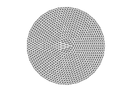
(a)

(b)

(c)

Figure 1: Meshes for $\mathcal{B}_{1}$.

Example 1

We consider the discretization of the Dirichlet problem (16) with $A=(-\Delta)^{s}$ and $f=1$ in the unit disk $\mathcal{B}_{1}\subset\mathbb{R}^{2}$. The exact solution for this problem is given by $u(x)=a_{n,s}(1-|x|^{2})^{s}$, where $a_{n,s}:=\dfrac{\mathsf{\Gamma}(n/2)}{2^{2s}\mathsf{\Gamma}(1+s)\mathsf{\Gamma}(s+n/2)}$. $\mathcal{B}_{1}$ is approximated by three meshes: quasi-uniform, $2$-graded, and adaptively generated triangular meshes as depicted in Figure 1. We consider fractional exponents $s=-\frac{1}{2},\frac{1}{4},\frac{7}{10},\frac{3}{4}$, to indicate the general applicability of our methods.

Tables 1–3 show the results of the Galerkin matrix $\mathbf{A}$ and its preconditioned form $\mathbf{P}\mathbf{A}$ for the different fractional exponents on the three families of meshes under consideration.

On all three classes of meshes, the condition number and the number of solver iterations for $\mathbf{A}$ show the expected strong growth when increasing $N$, while they are small and bounded for $\mathbf{P}\mathbf{A}$. We remark that the reduction of CG iterations achieved by our preconditioner is significant, with a higher reduction for larger $|s|$. Furthermore, $\kappa(\mathbf{P}\mathbf{A})$ remains almost constant across the refinement levels when $s=\frac{1}{4}$. We note, however, a very slow growth for $s=\frac{7}{10}$ and $s=\frac{3}{4}$ for the considered dofs. For $s=-\frac{1}{2}$ we obtain larger condition numbers consistent with previous observations hju . We note the larger condition number for the last data point on $2$-graded meshes of the preconditioned problem. We attribute this to a discretization error of the particular implementation. Even though we use the exact inverse on the unit disk to build our preconditioner, it is worth noticing that in this case $\mathbf{P}\mathbf{A}$ achieves only an approximate identity after discretization. This approximation error, together with the tolerance of $10^{-10}$ for the residual, explain why condition numbers and CG iteration counts are larger than 1.

Table 1: Condition numbers and CG iterations on quasi-uniform mesh (Figure 1a), Example 1.

	$s=-1/2$				$s=1/4$				$s=7/10$				$s=3/4$
N	$\mathbf{A}$		$\mathbf{P}\mathbf{A}$		$\mathbf{A}$		$\mathbf{P}\mathbf{A}$		$\mathbf{A}$		$\mathbf{P}\mathbf{A}$		$\mathbf{A}$		$\mathbf{P}\mathbf{A}$
	$\kappa$	It.	$\kappa$	It.	$\kappa$	It.	$\kappa$	It.	$\kappa$	It.	$\kappa$	It.	$\kappa$	It.	$\kappa$	It.
123	35.63	27	2.61	12	1.98	12	1.16	6	6.85	15	1.50	9	8.24	16	1.54	10
492	73.58	40	2.69	12	2.65	13	1.20	7	20.87	28	1.52	10	26.99	30	1.54	10
1968	153.95	56	2.74	13	4.11	16	1.25	7	62.10	47	1.56	10	87.24	51	1.72	11
7872	316.74	78	2.78	13	6.34	21	1.26	7	176.19	79	1.76	11	268.02	92	2.14	12
31488	643.01	131	2.83	14	9.36	27	1.28	7	478.78	135	1.93	11	784.22	160	2.57	12

Table 2: Condition numbers and CG iterations on $2$-graded mesh (Figure 1b), Example 1.

	$s=-1/2$				$s=1/4$				$s=7/10$				$s=3/4$
N	$\mathbf{A}$		$\mathbf{P}\mathbf{A}$		$\mathbf{A}$		$\mathbf{P}\mathbf{A}$		$\mathbf{A}$		$\mathbf{P}\mathbf{A}$		$\mathbf{A}$		$\mathbf{P}\mathbf{A}$
	$\kappa$	It.	$\kappa$	It.	$\kappa$	It.	$\kappa$	It.	$\kappa$	It.	$\kappa$	It.	$\kappa$	It.	$\kappa$	It.
123	35.63	27	2.61	12	8.41	20	1.14	6	4.53	16	1.72	11	5.17	16	1.94	12
1068	8190.98	255	4.92	20	23.33	36	1.21	7	28.33	32	2.42	14	33.57	34	2.92	14
4645	24657.62	431	6.17	22	41.63	44	1.25	7	106.53	70	2.85	14	133.26	75	3.65	15
13680	58165.89	620	9.25	26	63.52	48	1.27	7	282.57	99	2.97	14	364.14	116	3.87	16

Table 3: Condition numbers and CG iterations on adaptively generated meshes (Figure 1c), Example 1.

	$s=1/4$				$s=7/10$				$s=3/4$
N	$\mathbf{A}$		$\mathbf{P}\mathbf{A}$		$\mathbf{A}$		$\mathbf{P}\mathbf{A}$		$\mathbf{A}$		$\mathbf{P}\mathbf{A}$
	$\kappa$	It.	$\kappa$	It.	$\kappa$	It.	$\kappa$	It.	$\kappa$	It.	$\kappa$	It.
123	1.98	12	1.16	6	6.85	15	1.50	10	8.24	16	1.54	9
238	5.39	22	1.17	6	7.82	21	1.60	10	9.22	21	1.67	11
518	15.46	37	1.20	7	11.27	28	1.76	11	12.55	29	1.89	12
1098	45.30	58	1.21	7	17.53	37	1.83	11	18.15	38	2.01	12
2278	131.77	85	1.23	7	28.28	48	1.91	12	27.17	48	2.16	13
4658	386.95	121	1.26	8	46.65	65	2.00	12	41.48	61	2.35	14
9438	1138.72	165	1.27	8	78.41	85	2.08	13	64.30	77	2.50	14

To gain further insight about this small growth in $\kappa(\mathbf{P}\mathbf{A})$, we also inspect the eigenvalues of $\mathbf{A}$ and $\mathbf{P}\mathbf{A}$ for the two families of meshes where this behaviour is more notorious. These are displayed in Figure 2. We see in plots $(a),(c),(e)$ that the spectra on quasi-uniform meshes are as expected, while on graded meshes, plots $(b),(d),(f)$ reveal that the clustering of eigenvalues for the preconditioned matrix still increases slowly with the dofs. As the slope of this small growth tends to $0$ when augmenting the number of dofs, we attribute it to the preasymptotic regime.

(a)

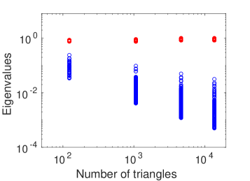
(b)

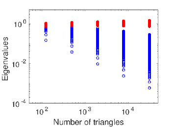
(c)

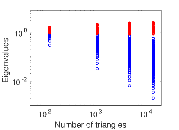
(d)

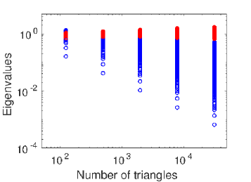
(e)

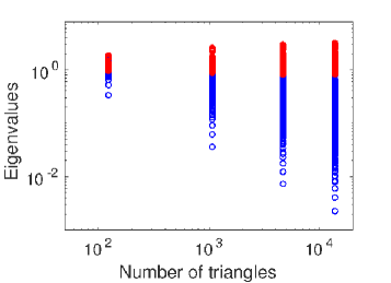
(f)

Figure 2: Eigenvalues of $\mathbf{A}$ (blue), resp. $\mathbf{P}\mathbf{A}$ (red), Example 1.

The next example illustrates the performance of the preconditioner defined by the bilinear form (18) on a domain bi-Lipschitz to $\mathcal{B}_{1}$.

Example 2

We consider the discretization of the Dirichlet problem (16) with $A=(-\Delta)^{s}$ and $f=1$ in the L-shaped domain $\Omega=[-1,3]^{2}\setminus[1,3]^{2}\subset\mathbb{R}^{2}$ depicted in Figure 4a. We examine fractional exponents $s=\frac{1}{4},\frac{1}{2},\frac{3}{4}$ on quasi-uniform, geometrically and algebraically graded meshes, see Figure 3 for an illustration. A numerical solution on a mesh with $3968$ elements is shown in Figure 4b. The preconditioner is computed using the radial projection $\chi$ from the L-shaped domain to $\mathcal{B}_{1}$. Here,

$$\chi:\Omega\to\mathcal{B}_{1},\quad\chi(x)=\frac{1}{r(x)}\frac{x}{|x|},$$

where $r(x):=\sup\{\lambda\in[1,\infty):\lambda x\in\Omega\}$.

Tables 4–7 display the results of the Galerkin matrix $\mathbf{A}$ and its preconditioned form $\mathbf{P}\mathbf{A}$ on a sequence of corresponding meshes. As in the unit disk $\mathcal{B}_{1}$ in Example 1, the condition number and the number of solver iterations for $\mathbf{A}$ show a strong increase with augmenting the dofs $N$, while the growth is small and of slope tending to $0$ for $\mathbf{P}\mathbf{A}$. We also note that the size of the condition numbers is slightly bigger than those from Example  1. This is a consequence of the fact that the preconditioner is no longer defined from an exact solution operator to the continuous problem, and thus the bound on the condition number is $h$-independent, yet larger than in the previous example. Indeed, as predicted by the theory, we see that the condition numbers and CG iterations obtained with the preconditioner remain small and bounded on quasi-uniform and geometrically graded meshes. However, the condition numbers of $\mathbf{P}\mathbf{A}$ for the algebraically graded meshes (Figure 3c) do not remain bounded. This is consistent with the theory, which applies to shape regular meshes, a condition not satisfied here. In order to illustrate this further, we also study a shape regular variant of the algebraically graded meshes (Figure 3d). The obtained results are reported in Table 7, which reveals that the condition numbers are bounded again. We point out that the assumptions of Theorem 5.1 are satisfied under certain mesh conditions introduced in Appendix A.2. The algebraically graded meshes from Figure 3c) violate the shape regularity condition $(C1)$ (and also condition $(C3)$ for $s=\frac{3}{4}$), while all other meshes considered verify all mesh conditions.

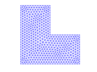
(a)

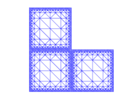
(b)

(c)

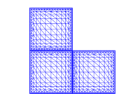
(d)

Figure 3: Meshes used for L-shaped domain, Example 2.

Table 4: Condition numbers and CG iterations on quasi-uniform meshes for L-shape (Figure 3a), Example 2.

	$s=1/4$				$s=1/2$				$s=3/4$
N	$\mathbf{A}$		$\mathbf{P}\mathbf{A}$		$\mathbf{A}$		$\mathbf{P}\mathbf{A}$		$\mathbf{A}$		$\mathbf{P}\mathbf{A}$
	$\kappa$	It.	$\kappa$	It.	$\kappa$	It.	$\kappa$	It.	$\kappa$	It.	$\kappa$	It.
248	2.35	15	1.24	8	4.00	16	1.48	9	8.90	23	2.35	12
992	2.86	16	1.27	8	8.22	24	1.58	9	26.22	40	2.68	13
3968	4.25	19	1.30	8	17.02	36	1.65	10	77.35	70	2.92	13
15872	6.73	24	1.32	8	35.00	52	1.69	10	226.56	118	3.11	14

Table 5: Condition numbers and CG iterations on $2$–graded (geometrically) meshes for L-shape (Figure 3b), Example 2.

	$s=1/4$				$s=1/2$				$s=3/4$
N	$\mathbf{A}$		$\mathbf{P}\mathbf{A}$		$\mathbf{A}$		$\mathbf{P}\mathbf{A}$		$\mathbf{A}$		$\mathbf{P}\mathbf{A}$
	$\kappa$	It.	$\kappa$	It.	$\kappa$	It.	$\kappa$	It.	$\kappa$	It.	$\kappa$	It.
288	4.28	20	1.24	8	7.08	21	1.51	9	14.06	26	2.36	13
720	12.53	34	1.29	8	18.65	34	1.60	10	35.02	38	2.46	14
1632	36.44	53	1.33	9	47.03	50	1.68	11	82.34	57	2.56	15
3504	105.28	76	1.37	9	114.49	76	1.75	11	185.29	83	2.67	15
7296	302.23	111	1.39	10	271.20	109	1.79	12	403.92	122	2.75	15
14928	862.91	162	1.39	10	628.32	155	1.76	11	859.51	172	2.84	15

Table 6: Condition numbers and CG iterations on $2$–graded (algebraically) meshes for L-shape (Figure 3c), Example 2.

	$s=1/4$				$s=1/2$				$s=3/4$
N	$\mathbf{A}$		$\mathbf{P}\mathbf{A}$		$\mathbf{A}$		$\mathbf{P}\mathbf{A}$		$\mathbf{A}$		$\mathbf{P}\mathbf{A}$
	$\kappa$	It.	$\kappa$	It.	$\kappa$	It.	$\kappa$	It.	$\kappa$	It.	$\kappa$	It.
384	12.49	34	1.36	9	8.91	28	1.78	12	28.72	37	4.30	22
1536	41.86	61	1.64	10	21.51	46	2.81	16	146.66	82	26.52	46
4704	105.76	94	1.94	12	47.29	67	3.76	18	559.48	159	91.34	161
16224	283.50	153	2.65	13	124.63	104	5.17	19	2726.63	486	695.92	443

Table 7: Condition numbers and CG iterations on $2$–graded (algebraically shape regular) meshes for L-shape (Figure 3d), Example 2.

	$s=1/4$				$s=1/2$				$s=3/4$
N	$\mathbf{A}$		$\mathbf{P}\mathbf{A}$		$\mathbf{A}$		$\mathbf{P}\mathbf{A}$		$\mathbf{A}$		$\mathbf{P}\mathbf{A}$
	$\kappa$	It.	$\kappa$	It.	$\kappa$	It.	$\kappa$	It.	$\kappa$	It.	$\kappa$	It.
528	13.12	36	1.28	8	12.99	31	1.67	11	25.12	33	2.64	15
912	19.15	44	1.30	8	19.78	37	1.71	11	42.33	43	2.87	16
2736	43.93	66	1.34	9	44.51	58	1.78	12	111.22	76	4.01	19
4920	63.79	79	1.36	9	67.06	73	1.79	12	183.65	99	4.22	19
9072	97.20	96	1.37	9	102.45	91	1.76	12	306.14	129	4.39	20
14784	140.13	114	1.38	9	142.72	108	1.73	11	458.32	161	4.49	20

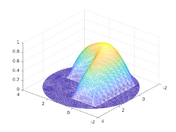
(a)

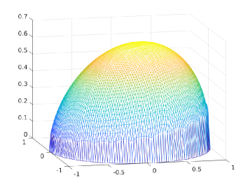
(b)

Figure 4: Numerical solutions for Example 2 $(a)$ and Example 4 $(b)$ with $s=\frac{3}{4}$.

Example 3

We consider the discretization of the Dirichlet problem (16) with $A=(-\Delta)^{s}$ and $f=1$ in rectangular domains $[-a,a]\times[-1,1]\subset\mathbb{R}^{2}$ with varying aspect ratio $a:1$. We examine fractional exponents $s=\frac{1}{4},\frac{1}{2},\frac{3}{4}$ on quasi-uniform meshes, see Figure 5 for illustration. The preconditioner is computed using the radial projection $\chi$ from the rectangular domain to $\mathcal{B}_{1}(0)$.

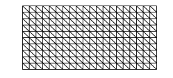
(a)

(b)

Figure 5: Meshes for rectangles with varied aspect ratio.

Tables 8–10 display the results of the Galerkin matrix $\mathbf{A}$ and its preconditioned form $\mathbf{P}\mathbf{A}$ on a sequence of corresponding meshes. In most cases, the preconditioner performs qualitatively the same as we already observed for Example 2: the condition numbers and the number of solver iterations for $\mathbf{P}\mathbf{A}$ tend to remain constant with respect to $h$.

The novelty here is how results change when the aspect ratio $a:1$ increases. Indeed, as expected from the theory, condition numbers, and consequently CG iteration counts, grow when the “distortion” from the unit disk is more significant, i.e. for bigger aspect ratios. Moreover, how the transformation impacts condition numbers depends on the related Sobolev norms, reason why they are actually $s$-dependent. This is clearly reflected in our experiments where the difference between the results when the aspect ratio is $1:1$ and $16:1$ is relatively small for $s=0.25$, but notorious for $s=0.75$. Nevertheless, as the original system for these distorted geometries are more ill-conditioned, $\mathbf{P}\mathbf{A}$ still reduces the number of iteration counts in a meaningful manner.

Although it is hard to draw general conclusions, with these results we expect to convey two messages: On the one hand, we highlight the robustness of this preconditioning approach. On the other hand, we warn the reader that there may be geometries for which, despite of the quasi-uniform mesh on the original geometry, “the mapping trick” from (18) can lead to large, yet bounded, condition numbers and thereby may no longer be a practical strategy to construct a preconditioner.

Table 8: Condition numbers and CG iterations on quasi-uniform mesh with $s=0.25$ and varied aspect ratio $a:1$, Example 3.

	$1:1$				$2:1$				$4:1$				$8:1$				$16:1$
$h$	$\mathbf{A}$		$\mathbf{P}\mathbf{A}$		$\mathbf{A}$		$\mathbf{P}\mathbf{A}$		$\mathbf{A}$		$\mathbf{P}\mathbf{A}$		$\mathbf{A}$		$\mathbf{P}\mathbf{A}$		$\mathbf{A}$		$\mathbf{P}\mathbf{A}$
	$\kappa$	It.	$\kappa$	It.	$\kappa$	It.	$\kappa$	It.	$\kappa$	It.	$\kappa$	It.	$\kappa$	It.	$\kappa$	It.	$\kappa$	It.	$\kappa$	It.
$\frac{1}{5\sqrt{2}}$	1.90	12	1.98	11	2.06	12	2.05	11	2.22	12	2.16	12	2.30	13	2.29	12	2.34	14	2.43	13
$\frac{1}{10\sqrt{2}}$	2.54	12	2.05	11	2.91	13	2.12	12	3.14	14	2.25	12	3.26	16	2.41	13	3.32	18	2.56	14
$\frac{1}{15\sqrt{2}}$	3.11	13	2.09	12	3.57	15	2.15	12	3.85	16	2.28	12	4.00	19	2.45	13	4.15	20	2.62	14
$\frac{1}{20\sqrt{2}}$	3.59	14	2.10	12	4.12	16	2.17	12	4.45	18	2.31	12	4.62	20	2.49	14	4.78	21	2.67	14

Table 9: Condition numbers and CG iterations on quasi-uniform mesh with $s=0.50$ and varied aspect ratio $a:1$, Example 3.

	$1:1$				$2:1$				$4:1$				$8:1$				$16:1$
$h$	$\mathbf{A}$		$\mathbf{P}\mathbf{A}$		$\mathbf{A}$		$\mathbf{P}\mathbf{A}$		$\mathbf{A}$		$\mathbf{P}\mathbf{A}$		$\mathbf{A}$		$\mathbf{P}\mathbf{A}$		$\mathbf{A}$		$\mathbf{P}\mathbf{A}$
	$\kappa$	It.	$\kappa$	It.	$\kappa$	It.	$\kappa$	It.	$\kappa$	It.	$\kappa$	It.	$\kappa$	It.	$\kappa$	It.	$\kappa$	It.	$\kappa$	It.
$\frac{1}{5\sqrt{2}}$	4.35	14	1.81	11	5.64	17	1.92	11	6.37	20	2.25	12	6.68	23	2.74	13	6.80	27	3.41	15
$\frac{1}{10\sqrt{2}}$	8.70	20	1.83	11	11.30	25	1.96	12	12.79	30	2.32	13	13.42	35	2.91	15	13.72	40	3.64	17
$\frac{1}{15\sqrt{2}}$	13.07	25	1.84	11	16.98	31	1.97	11	19.22	37	2.36	13	20.19	45	2.99	15	20.63	49	3.77	17
$\frac{1}{20\sqrt{2}}$	17.44	29	1.85	11	22.66	36	1.99	12	25.66	42	2.39	14	26.97	52	3.05	15	27.48	54	3.86	17

Table 10: Condition numbers and CG iterations on quasi-uniform mesh with $s=0.75$ and varied aspect ratio $a:1$, Example 3.

	$1:1$				$2:1$				$4:1$				$8:1$				$16:1$
$h$	$\mathbf{A}$		$\mathbf{P}\mathbf{A}$		$\mathbf{A}$		$\mathbf{P}\mathbf{A}$		$\mathbf{A}$		$\mathbf{P}\mathbf{A}$		$\mathbf{A}$		$\mathbf{P}\mathbf{A}$		$\mathbf{A}$		$\mathbf{P}\mathbf{A}$
	$\kappa$	It.	$\kappa$	It.	$\kappa$	It.	$\kappa$	It.	$\kappa$	It.	$\kappa$	It.	$\kappa$	It.	$\kappa$	It.	$\kappa$	It.	$\kappa$	It.
$\frac{1}{5\sqrt{2}}$	13.16	22	1.70	11	19.06	30	1.99	12	22.13	37	3.62	14	23.23	44	11.56	17	23.60	53	39.03	25
$\frac{1}{10\sqrt{2}}$	37.19	37	1.75	12	53.94	51	2.05	14	62.68	62	3.99	16	65.87	76	17.33	20	67.36	91	18.12	30
$\frac{1}{15\sqrt{2}}$	68.36	50	1.81	13	99.16	68	2.11	15	115.27	83	4.21	17	121.21	103	21.58	22	123.93	124	20.09	34
$\frac{1}{20\sqrt{2}}$	105.28	62	1.87	14	152.74	85	2.15	15	177.61	107	4.35	18	186.92	129	24.94	24	189.17	147	21.84	36

As a final example, we apply the preconditioner to a non-symmetric model problem motivated by the fractional Patlak-Keller-Segel equation for chemotaxis egp .

Example 4

We consider the discretization of the Dirichlet problem (16) with $A=(-\Delta)^{s}+c\cdot\nabla$, $c=(0.3,0)^{T}$ and $f=1$ on the unit disk $\mathcal{B}_{1}\subset\mathbb{R}^{2}$ with $s=\frac{1}{2}$, $s=\frac{7}{10}$ and $s=\frac{3}{4}$. Quasi-uniform and algebraically $2$-graded meshes are considered. A numerical solution on a uniform mesh with 7872 elements is depicted in Figure 4.

Tables 11 and 12 display the condition numbers of the Galerkin matrix $\mathbf{A}$ and its preconditioned form $\mathbf{P}\mathbf{A}$ for the different fractional exponents on sequences of quasi-uniform meshes, and on algebraically graded meshes. The number of GMRES iterations is given for this non-symmetric problem.

As in the earlier examples, on both quasi-uniform and graded meshes the condition number and the number of solver iterations for $\mathbf{A}$ show a strong increase with $N$. For $\mathbf{P}\mathbf{A}$ they are bounded with a slight growth, with numbers very close to those in Example 1 for $s=\frac{7}{10},\frac{3}{4}$. Note that for $s=\frac{1}{2}$ the gradient term is of the same order as $(-\Delta)^{s}$.

Table 11: Condition numbers and GMRES iterations on quasi-uniform mesh, Example 4.

	$s=1/2$				$s=7/10$				$s=3/4$
N	$\mathbf{A}$		$\mathbf{P}\mathbf{A}$		$\mathbf{A}$		$\mathbf{P}\mathbf{A}$		$\mathbf{A}$		$\mathbf{P}\mathbf{A}$
	$\kappa$	It.	$\kappa$	It.	$\kappa$	It.	$\kappa$	It.	$\kappa$	It.	$\kappa$	It.
123	3.11	14	1.08	12	6.69	17	1.48	11	8.11	18	1.49	11
492	7.02	22	1.15	12	20.39	29	1.50	11	26.59	32	1.53	11
1968	15.08	35	1.19	12	60.87	48	1.54	11	85.93	55	1.71	11
7872	31.85	54	1.22	13	172.73	83	1.77	11	264.01	95	2.15	12

Table 12: Condition numbers and GMRES iterations on graded mesh, Example 4.

	$s=1/2$				$s=7/10$				$s=3/4$
N	$\mathbf{A}$		$\mathbf{P}\mathbf{A}$		$\mathbf{A}$		$\mathbf{P}\mathbf{A}$		$\mathbf{A}$		$\mathbf{P}\mathbf{A}$
	$\kappa$	It.	$\kappa$	It.	$\kappa$	It.	$\kappa$	It.	$\kappa$	It.	$\kappa$	It.
123	3.31	19	1.17	12	4.42	17	1.70	12	5.07	18	1.93	12
1068	14.24	31	1.26	12	27.78	36	2.39	14	33.07	38	2.91	15
4645	44.15	54	1.34	12	104.49	69	2.84	15	131.43	79	3.64	16
13680	101.41	73	1.37	12	277.05	103	2.96	15	358.78	117	3.87	16

Appendix A Proof of Results for Operator Preconditioning on Adaptive Meshes

For the sake of presentation, we dedicate the next two subsections to briefly summarize some key concepts about adaptivity and the mesh conditions we need to fulfill for stability. Finally, we combine these preliminaries to state and and prove the new results on operator preconditioning in adaptively refined meshes.

A.1 Adaptivity preliminaries

We begin by reminding the reader of some of the concepts introduced in Section 5.2. Given an initial triangulation $\mathcal{T}_{h}^{(0)}$, the adaptive Algorithm A generates a sequence $\mathcal{T}_{h}^{(\ell)}$ of triangulations based on error indicators $\eta^{(\ell)}(\tau),\;\tau\in\mathcal{T}_{h}^{(\ell)}$, a refinement criterion and a refinement rule, by following the established sequence of steps:

$$\mathrm{SOLVE}\to\mathrm{ESTIMATE}\to\mathrm{MARK}\to\mathrm{REFINE}.$$

There are different refinement rules that one can choose for the step REFINE. We now present some of the most common ones: red refinement, green refinement, and red-green refinement.

Definition 1

Let $\mathcal{T}_{h}^{(\ell)}$ be a triangulation. A triangle $\tau\in\mathcal{T}_{h}^{(\ell)}$ is red refined by connecting edge midpoints of $\tau$, thus splitting $\tau$ into 4 similar triangles.

Definition 2

Let $\mathcal{T}_{h}^{(\ell)}$ be a triangulation. A triangle $\tau\in\mathcal{T}_{h}^{(\ell)}$ is green refined by connecting an edge midpoint with the opposite vertex of $\tau$, thus splitting $\tau$ into 2 triangles.

Next, in order to define a red-green refinement, we introduce two related properties.

Definition 3

1. A triangulation $\mathcal{T}_{h}^{(\ell)}$ is called $1$–irregular if the property

   $$|\operatorname{lev}(\tau_{k})-\operatorname{lev}(\tau_{m})|\leq 1,$$

   holds for any pair of triangles $\tau_{k},\tau_{m}\in\mathcal{T}_{h}^{(\ell)}$ such that $\tau_{k}\cap\tau_{m}\neq\emptyset$.

   Here $\operatorname{lev}(\tau_{k})$ corresponds to the number of refinement steps required to generate $\tau_{k}$ from the initial triangulation $\mathcal{T}_{h}^{(0)}$.
   

2. The $2$–neighbour rule: Red refine any triangle $\tau_{k}$ with $2$ neighbours that have been red refined. Two triangles are neighbours, if they have a common edge.

Definition 4

A Red-green refinement for a triangulation $\mathcal{T}_{h}^{(\ell)}$ proceeds as follows:

1. Remove edges from any triangles that have been green refined.

2. All marked triangles are red refined.

3. Any triangles with 2 or more red refined neighbours are red refined, by $2$–neighbour rule.

4. Any triangles that do not fulfil $1$–irregularity rule are further refined.

5. Any triangles with hanging nodes generated during the refinement are green refined.

For further description of the refinement rules, we refer to bsw ; jg .

Figure 6: Example of red refined triangle (left) and green refined triangle (right).

Figure 7: Example of a sequence of red-green refinement. Top element is marked by $(o)$ and therefore is red refined in the first step. Bottom triangle then has a hanging node and is green refined in the consequent step.

A.2 Mesh conditions

We recall that we aim to show (20), i.e.

$$\underset{\varphi_{h}\in\mathbb{W}_{h}}{\mathrm{sup}}\dfrac{\mathsf{d}(v_{h},\varphi_{h})}{\|\varphi_{h}\|_{H^{-s}(\Omega)}}\geq{\color[rgb]{0,0,0}\beta_{\mathsf{d}}}\|v_{h}\|_{\widetilde{H}^{s}(\Omega)},\qquad\text{for all }v_{h}\in\widetilde{\mathbb{V}}_{h},$$

(see Section 5 for notation).

In the case of the discretizations based on dual meshes, this inf-sup stability is a consequence of three regularity conditions on the triangulation $\mathcal{T}_{h}$, see (s2, , Chapters 1–2). We now proceed to introduce some notation to properly summarize this result.

Let $\mathcal{T}_{h}$ be a triangulation of $\Omega\subset\mathbb{R}^{n}$. For each triangle $\tau_{k}\in\mathcal{T}_{h}$ we define its area $\Delta_{k}:=\int_{\tau_{k}}dx$; its local element size $h_{k}:=\Delta_{k}^{1/n}$; and its diameter $d_{k}:=\sup_{x,y\in\tau_{k}}|x-y|$.

Let $\varphi_{j}$ be a piecewise linear basis function in the span of $\widetilde{\mathbb{V}}_{h}$. We write $\omega_{j}:=\operatorname{supp}\,\varphi_{j}$ and define its associated local mesh size $\hat{h}_{j}$ as

$$\hat{h}_{j} :=\frac{1}{\#I(j)}\sum_{m\in I(j)}h_{m}.$$

Here, $I(j):=\left\{m\in\{1,\ldots,\#\mathcal{T}_{h}\}:\tau_{m}\cap\omega_{j}\neq\emptyset\right\},\text{ for }j=1,\ldots,N,$ is the index set of triangles $\tau_{m}\in\mathcal{T}_{h}$ where the basis function $\varphi_{j}$ is not identically zero.

Definition 5

For a triangulation $\mathcal{T}_{h}$, we define the following mesh conditions

• Shape regularity: there exists $c_{R}>0$ such that for all $\tau_{k}\in\mathcal{T}_{h}$

  $$0<c_{R}<\frac{h_{k}}{d_{k}}<1.$$

• Local quasi-uniformity: for all $\tau_{k},\tau_{m}\in\mathcal{T}$ with $\tau_{k}\cap\tau_{m}\neq\emptyset$

  $$\frac{h_{k}}{h_{m}}\leq c_{L},$$

  with $C_{L}$ a (uniform) positive constant.

• Local $s$-dependent condition: there exists $c_{0}>0$ such that for all $\tau\in\mathcal{T}_{h}$

  $$\frac{51}{7}-\sqrt{\sum_{j\in J(m)}\hat{h}_{j}^{2s}\sum_{j\in J(m)}\hat{h}_{j}^{-2s}}\geq c_{0}>0,$$

  with $J(m):=\left\{i\in\{1,\ldots,N\}:\omega_{i}\cap\tau_{m}\neq\emptyset\right\}$ for $m=1,\ldots,\#\mathcal{T}_{h}$, the index set of basis functions $\varphi_{i}$ which are not identically zero on triangle $\tau_{m}$.

Theorem A.1 ((s, , Theorems 2.1 and 2.2))

Let $\mathcal{T}_{h}$ be a triangulation of $\Omega$ such that $(C1),(C2)$ and $(C3)$ are satisfied. Consider the primal-dual discretization $\widetilde{\mathbb{V}}_{h}=\mathbb{S}^{1}(\mathcal{T}_{h})\cap\widetilde{H}^{s}(\Omega)$ and $\mathbb{W}_{h}=\mathbb{S}^{0}(\check{\mathcal{T}}_{h})$ for $0\leq s\leq 1$ (see subsection 5.1).

Then, the discrete inf-sup condition (20) holds with a positive constant $\beta_{\mathsf{d}}$ independent of $h$.

A.3 Results on adaptively refined meshes

Now we turn our attention to study these conditions for a sequence of adaptive triangulations generated by Algorithm A. For this, we write the constants from conditions (C1), (C2) and (C3) associated to a triangulation $\mathcal{T}_{h}^{(\ell)}$ as $c_{R}^{(\ell)},c_{L}^{(\ell)}$ and $c_{0}^{(\ell)}$, respectively.

The next Lemma is the complete version of Lemma 5 introduced in Section 5.2.

Lemma 6

Consider an initial triangulation $\mathcal{T}_{h}^{(0)}$ satisfying the mesh conditions from Definition 5, and such that its local quasi-uniformity constant $c_{L}^{(0)}$ verifies

$$c_{L}^{(0)}\leq\frac{1}{2}\sqrt[4|s|]{\frac{1129}{49}}\approx\frac{2.19^{1/|s|}}{2}.$$ (27)

Let $\Xi:=\{\mathcal{T}_{h}^{(\ell)}\}_{\ell\in\operatorname{\mathbb{N}}}$ be a family of meshes generated from $\mathcal{T}_{h}^{(0)}$ by the adaptive refinement described in Algorithm A, using red-green refinements. Then (C1), (C2) and (C3) hold for all $\mathcal{T}_{h}^{(\ell)}\in\Xi$ for some constants $c_{R},c_{L},c_{0}>0$, which are independent of $\ell\in\mathbb{N}$.

In particular, the inf-sup condition (20) holds for $|s|\leq 1$, $\widetilde{\mathbb{V}}_{h}=\mathbb{S}^{p}(\mathcal{T}_{h})\cap\widetilde{H}^{s}(\Omega)$, $\mathbb{W}_{h}=\mathbb{S}^{q}(\mathcal{T}_{h}^{\prime})$, and for all $\mathcal{T}_{h}^{(\ell)}$ independent of $\ell$.

Proof

The proof proceeds by induction on $\ell$. By hypothesis, the initial triangulation $\mathcal{T}_{h}^{(0)}$ satisfies $(C1)$ and $(C2)$. Therefore, for the initial triangulation $\mathcal{T}_{h}^{(0)}$ we only need to check $(C3)$.

For the sake of convenience, let us re-label the basis functions $j\in J(m)$ by $m_{i}$, with $i=1,\ldots,\#J(m)$. We note that $\max_{m}\#J(m)=3$ and that this is our worst case scenario. Therefore, it suffices to verify $(C3)$ in this case:

$$\frac{51}{7}-\sqrt{\sum_{i=1}^{3}\hat{h}_{m_{i}}^{2s}\sum_{i=1}^{3}\hat{h}_{m_{i}}^{-2s}}\geq c_{0}>0.$$

Without loss of generality, let $\hat{h}_{m_{1}}\geq\hat{h}_{m_{2}}\geq\hat{h}_{m_{3}}$. Then

$$\begin{split}\sum_{i=1}^{3}\hat{h}_{m_{i}}^{2s}\sum_{i=1}^{3}\hat{h}_{m_{i}}^{-2s}&=\textstyle{3+\left(\frac{\hat{h}_{m_{1}}}{\hat{h}_{m_{2}}}\right)^{2|s|}+\left(\frac{\hat{h}_{m_{2}}}{\hat{h}_{m_{3}}}\right)^{2|s|}+\left(\frac{\hat{h}_{m_{3}}}{\hat{h}_{m_{1}}}\right)^{2|s|}}\\ &\qquad+\textstyle{\left(\frac{\hat{h}_{m_{1}}}{\hat{h}_{m_{3}}}\right)^{2|s|}+\left(\frac{\hat{h}_{m_{2}}}{\hat{h}_{m_{1}}}\right)^{2|s|}+\left(\frac{\hat{h}_{m_{3}}}{\hat{h}_{m_{2}}}\right)^{2|s|}}\\ &\leq 3+\textstyle{2\left(\left(\frac{\hat{h}_{m_{1}}}{\hat{h}_{m_{3}}}\right)^{2|s|}+\left(\frac{\hat{h}_{m_{2}}}{\hat{h}_{m_{2}}}\right)^{2|s|}+\left(\frac{\hat{h}_{m_{3}}}{\hat{h}_{m_{1}}}\right)^{2|s|}\right)\leq 7+2\left(\frac{\hat{h}_{m_{1}}}{\hat{h}_{m_{3}}}\right)^{2|s|},}\\ \end{split}$$

where we use the rearrangement inequality. We conclude that $(C3)$ is satisfied for $\mathcal{T}_{h}^{(0)}$ provided that

$$\textstyle{\left(\frac{\hat{h}_{m_{1}}}{\hat{h}_{m_{3}}}\right)^{2|s|}<\frac{1129}{49}.}$$ (28)

A simple calculation using the mesh conditions yields $\frac{\hat{h}_{m_{1}}}{\hat{h}_{m_{3}}}\leq(c_{L}^{(0)})^{2}$, so that (28) holds and $(C3)$ is satisfied for $\mathcal{T}_{h}^{(0)}$.
For the inductive step, assume that conditions $(C1)$–$(C3)$ are satisfied on an adaptively refined triangulation $\mathcal{T}_{h}^{(\ell)}$ using red-green refinements subject to $1$–irregularity and $2$–neighbour rules. In order to generate a new triangulation $\mathcal{T}_{h}^{(\ell+1)}$, the appropriate triangles are marked.

We note that red-refinement does not change the shape regularity constant, but green refinement worsens the shape regularity constant by at most a factor of $\frac{1}{\sqrt{2}}$. However, due to the removal of green edges, the constant does not degenerate as $\ell\to\infty$. Thus condition $(C1)$ is satisfied with $c_{R}^{(\ell+1)}\geq\frac{1}{\sqrt{2}}c_{R}^{(0)}$ for $\mathcal{T}_{h}^{(\ell+1)}$.

Condition $(C2)$ remains satisfied due to the $1$–irregularity condition in the refinement procedure. This restriction guarantees that $\frac{h_{i}}{h_{j}}\leq c_{L}^{(\ell+1)}\leq 2c_{L}^{(0)}$.

As for the initial triangulation $\mathcal{T}_{h}^{(0)}$, we know that condition $(C3)$ is satisfied for $\mathcal{T}_{h}^{(\ell+1)}$ when (28) holds. Due to the $1$–irregularity condition, we have that $\frac{\hat{h}_{m_{1}}}{\hat{h}_{m_{3}}}\leq(2c_{L}^{(0)})^{2}$, so the estimate (28) is satisfied provided $c_{L}^{(0)}<\frac{1}{2}{\left(\frac{1129}{49}\right)}^{{1}/{4|s|}}$.

We conclude that $(C1)$, $(C2)$, $(C3)$ are satisfied for $\{\mathcal{T}_{h}^{(\ell)}\}_{\ell=0}^{\infty}$ independently of $\ell$. ∎

Remark 9

1. We note that the estimates in Lemma 6 are not sharp. Still, the local quasi-uniformity assumption on the initial triangulation $\mathcal{T}^{(0)}$ becomes more restrictive as $|s|$ increases. Thus, the initial mesh needs to be of increasingly higher regularity for higher values of $|s|$.

2. Let $\Gamma{\color[rgb]{0,0,0}\subset}\mathbb{R}^{n}$ be a polyhedral domain which satisfies an interior cone condition. Then the assumptions in Lemma 6 can be satisfied for a sufficiently fine $\mathcal{T}_{h}^{(0)}$.

Remark 10

Similar results can be shown for alternative refinement strategies, such as the newest vertex bisection (dirk_nvb, , Section 2.2). See (jsthesis, , Chapter 4) for details.

Appendix B Proof of Proposition 2

The idea for the proof is like in CHR02 where the case $\mathbb{W}_{h}=\widetilde{\mathbb{V}}_{h}$ is shown. Here we generalize the proof to different discrete test and trial space. For the sake of brevity we will discuss the case when $s\in(1/2,1]$ and remark that the proof for $s\in[-1,-1/2)$ follows analogously. We remind the reader that in this setting $\widetilde{H}^{s}(\Omega)\equiv H^{s}_{0}(\Omega)\neq H^{s}(\Omega)$, but that $\|u\|_{\widetilde{H}^{s}(\Omega)}\equiv\|u\|_{{H}^{s}(\Omega)},\>\forall u\in\widetilde{H}^{s}(\Omega)$.

Let $\mathcal{T}_{h}$, $\mathbb{S}^{p}(\mathcal{T}_{h}),p\in\operatorname{\mathbb{N}}$ be as in Section 5. Moreover, we recall that for this setting we consider the finite element spaces $\widetilde{\mathbb{V}}_{h}=\mathbb{S}^{1}(\mathcal{T}_{h})\cap\widetilde{H}^{s}(\Omega)$ and $\mathbb{W}_{h}\subset{H}^{-s}(\Omega)$. Additionally, we denote $\mathbb{V}_{h}=\mathbb{S}^{1}(\mathcal{T}_{h})\subset{H}^{s}(\Omega)$ and note that $\widetilde{\mathbb{V}}_{h}\subset\mathbb{V}_{h}$. Indeed, $\widetilde{\mathbb{V}}_{h}$ is the space of affine continuous functions that are zero on the boundary, while $\mathbb{V}_{h}$ is analogous to $\widetilde{\mathbb{V}}_{h}$, but admits non-zero values on $\partial\Omega$.

Let us introduce the generalized $L^{2}$-projection $\widetilde{Q}_{h}:L^{2}(\Omega)\to\widetilde{\mathbb{V}}_{h}$ for a given $u\in L^{2}(\Omega)$, as the solution of the variational problem

$$\left\langle\widetilde{Q}_{h}u\,,\,\psi_{h}\right\rangle_{\Omega}=\left\langle u\,,\,\psi_{h}\right\rangle_{\Omega},\quad\forall\psi_{h}\in\mathbb{W}_{h}.$$ (29)

From (s2, , Chapter 2), hut , we know that it satisfies

$$\|\widetilde{Q}_{h}u\|_{\widetilde{H}^{s}(\Omega)}\leq{\color[rgb]{0,0,0}\beta_{\mathsf{d}}^{-1}}\|u\|_{\widetilde{H}^{s}(\Omega)},\qquad\forall u\in\widetilde{H}^{s}(\Omega).$$ (30)

where ${\color[rgb]{0,0,0}\beta_{\mathsf{d}}}$ is the inf-sup constant from (20).

Given that we are interested in the case where we have a space mismatch, i.e. when $u\in H^{s}(\Omega)$ but $u\notin\widetilde{H}^{s}(\Omega)$, we additionally prove the following:

Lemma 7

The projection $\widetilde{Q}_{h}$ satisfies

$$\|\widetilde{Q}_{h}u_{h}\|_{H^{s}(\Omega)}\leq(1+{\color[rgb]{0,0,0}\frac{c_{2}}{s-{1/2}}}\,h^{1/2-s})\|u_{h}\|_{H^{s}(\Omega)},\qquad\forall u_{h}\in\mathbb{V}_{h},$$ (31)

with $c_{2}>0$ and independent of $h$.

Proof

Set $u^{0}_{h}\in\widetilde{\mathbb{V}}_{h}$ to be the function defined by

$$u^{0}_{h}:=\begin{cases}u_{h},\quad\text{ in all interior nodes},\\ 0,\qquad\text{on }\partial\Omega.\end{cases}$$ (32)

Then, by definition

$$\|u_{h}-\widetilde{Q}_{h}u_{h}\|_{L^{2}(\Omega)} =\|u_{h}-u_{h}^{0}\|_{L^{2}(\Omega)}\leq h^{1/2}\|u_{h}\|_{L^{2}(\partial\Omega)},$$

where the last inequality holds by basic computations (c.f. (CHR02, , Equation 1.3.27)).

From the trace theorem, we have that $\|u_{h}\|_{L^{2}(\partial\Omega)}\leq\dfrac{c_{tt}}{s-1/2}\|u_{h}\|_{H^{s}(\Omega)}$, with $c_{tt}>0$ independent of $h$.

Therefore, combining all the above, we obtain

$$\|\widetilde{Q}_{h}u_{h}\|_{H^{s}(\Omega)} \leq\|u_{h}\|_{H^{s}(\Omega)}+\|\widetilde{Q}_{h}u_{h}-u_{h}\|_{H^{s}(\Omega)}$$

$$\leq\|u_{h}\|_{H^{s}(\Omega)}+{\color[rgb]{0,0,0}c_{1}}h^{-s}\|\widetilde{Q}_{h}u_{h}-u_{h}\|_{L^{2}(\Omega)}$$

$$\leq\left(1+\frac{{\color[rgb]{0,0,0}c_{1}c_{tt}}}{s-1/2}h^{1/2-s}\right)\|u_{h}\|_{H^{s}(\Omega)}.$$

∎

Now, let us also introduce the finite element space $\widetilde{\mathbb{W}}_{h}\subset\widetilde{H}^{-s}(\Omega)$. We consider the generalized $L^{2}$-projection $\widetilde{P}_{h}:L^{2}(\Omega)\to\widetilde{\mathbb{W}}_{h}$ for a given $\varphi\in L^{2}(\Omega)$, as the solution of the variational problem

$$\left\langle\widetilde{P}_{h}\varphi\,,\,v_{h}\right\rangle_{\Omega}=\left\langle\varphi\,,\,v_{h}\right\rangle_{\Omega},\quad\forall v_{h}\in\mathbb{V}_{h}.$$ (33)

Then, in analogy with Lemma 7, we have that

Lemma 8

The projection $\widetilde{P}_{h}$ satisfies

$$\|\widetilde{P}_{h}\Phi_{h}\|_{H^{-s}(\Omega)}\leq c_{3}(1+{\color[rgb]{0,0,0}\frac{c_{2}}{s-{1/2}}}\,h^{1/2-s})\|\Phi_{h}\|_{H^{-s}(\Omega)},\qquad\forall\Phi_{h}\in\mathbb{W}_{h},$$ (34)

with $c_{2},c_{3}>0$ and independent of $h$.

Proof

Let us use the norms’ properties and write

$$\|\widetilde{P}_{h}\Phi_{h}\|_{H^{-s}(\Omega)}\leq\|\widetilde{P}_{h}\Phi_{h}\|_{\widetilde{H}^{-s}(\Omega)}=\underset{0\neq u\in H^{s}(\Omega)}{\mathrm{sup}}\dfrac{\left\langle\widetilde{P}_{h}\Phi_{h}\,,\,u\right\rangle_{\Omega}}{\|u\|_{H^{s}(\Omega)}}.$$

Then, using the definition of $\widetilde{Q}_{h}$ and the estimates above, we get

$$\|\widetilde{P}_{h}\Phi_{h}\|_{H^{-s}(\Omega)} \leq(1+{\color[rgb]{0,0,0}\frac{c_{2}}{s-{1/2}}}\,h^{1/2-s})\underset{0\neq u\in H^{s}(\Omega)}{\mathrm{sup}}\dfrac{\left\langle\widetilde{P}_{h}\Phi_{h}\,,\,\widetilde{Q}_{h}u\right\rangle_{\Omega}}{\|\widetilde{Q}_{h}u\|_{H^{s}(\Omega)}}$$

$$\leq(1+{\color[rgb]{0,0,0}\frac{c_{2}}{s-{1/2}}}\,h^{1/2-s})\underset{0\neq u_{h}\in\widetilde{\mathbb{V}}_{h}}{\mathrm{sup}}\dfrac{\left\langle\widetilde{P}_{h}\Phi_{h}\,,\,u_{h}\right\rangle_{\Omega}}{\|u_{h}\|_{H^{s}(\Omega)}}.$$

Now, by definition of $\widetilde{P}_{h}$, and since $\widetilde{\mathbb{V}}_{h}\subset\mathbb{V}_{h}$, we have

$$\|\widetilde{P}_{h}\Phi_{h}\|_{H^{-s}(\Omega)} \leq(1+{\color[rgb]{0,0,0}\frac{c_{2}}{s-{1/2}}}\,h^{1/2-s}\,)\underset{0\neq u_{h}\in\widetilde{\mathbb{V}}_{h}}{\mathrm{sup}}\dfrac{\left\langle\Phi_{h}\,,\,u_{h}\right\rangle_{\Omega}}{\|u_{h}\|_{H^{s}(\Omega)}}$$

$$\leq{\color[rgb]{0,0,0}c_{3}}(1+{\color[rgb]{0,0,0}\frac{c_{2}}{s-{1/2}}}\,h^{1/2-s}\,)\|\Phi_{h}\|_{H^{-s}(\Omega)}.$$

∎

Lemma 9

Let $s\in(1/2,1)$. Then, the following inf-sup condition holds

$$\underset{\phi_{h}\in\widetilde{\mathbb{W}}_{h}}{\mathrm{sup}}\dfrac{\left\langle v_{h}\,,\,\phi_{h}\right\rangle_{\Omega}}{\|\phi_{h}\|_{H^{-s}(\Omega)}}\geq{\color[rgb]{0,0,0}\frac{\beta_{\mathsf{d}}}{c_{3}}}\left(1+{\color[rgb]{0,0,0}\frac{c_{2}}{s-{1/2}}}\,h^{1/2-s}\right)^{-1}\|v_{h}\|_{\widetilde{H}^{s}(\Omega)},\quad\forall v_{h}\in\widetilde{\mathbb{V}}_{h},$$ (35)

with ${\color[rgb]{0,0,0}c_{3},c_{2}}>0$ and independent of $h$.

Proof

Let us introduce the operator $\Pi_{h}^{s}:\widetilde{H}^{s}(\Omega)\to\mathbb{W}_{h}\subset H^{-s}(\Omega)$ for $s\in(0,1]$, defined by the variational formulation

$$\left\langle\Pi_{h}^{s}u\,,\,v_{h}\right\rangle_{\Omega}=(u,v_{h})_{\widetilde{H}^{s}(\Omega)},\quad\forall v_{h}\in\widetilde{\mathbb{V}}_{h},$$ (36)

where $(\cdot,\cdot)_{\widetilde{H}^{s}(\Omega)}$ denotes the $\widetilde{H}^{s}(\Omega)$-inner product. This operator is analogous to (s2, , Equation 1.75) (hju, , Equation 4.22), and thus it verifies

$$\|\Pi_{h}^{s}u\|_{{H}^{-s}(\Omega)}\leq{\color[rgb]{0,0,0}\beta_{\mathsf{d}}^{-1}}\|u\|_{\widetilde{H}^{s}(\Omega)},\qquad\forall u\in\widetilde{H}^{s}(\Omega).$$ (37)

Next, we have that for any $v_{h}\in\widetilde{\mathbb{V}}_{h}$

$$\|v_{h}\|_{\widetilde{H}^{s}(\Omega)} =\dfrac{(v_{h},v_{h})_{\widetilde{H}^{s}(\Omega)}}{\|v_{h}\|_{\widetilde{H}^{s}(\Omega)}}=\dfrac{\left\langle v_{h}\,,\,\Pi_{h}v_{h}\right\rangle_{\Omega}}{\|v_{h}\|_{\widetilde{H}^{s}(\Omega)}}\leq\beta_{\mathsf{d}}^{-1}\dfrac{\left\langle v_{h}\,,\,\Pi_{h}v_{h}\right\rangle_{\Omega}}{\|\Pi_{h}v_{h}\|_{H^{-s}(\Omega)}}=\beta_{\mathsf{d}}^{-1}\dfrac{\left\langle v_{h}\,,\,\widetilde{P}_{h}\Pi_{h}v_{h}\right\rangle_{\Omega}}{\|\Pi_{h}v_{h}\|_{{H}^{-s}(\Omega)}},$$

where in the last step we used that $\Pi_{h}v_{h}\in\mathbb{W}_{h}$ and the definition of $\widetilde{P}_{h}$.

Now, let us use our previous estimates to derive

$$\|v_{h}\|_{\widetilde{H}^{s}(\Omega)}\leq\frac{c_{3}}{\beta_{\mathsf{d}}}(1+\frac{c_{2}}{s-1/2}\,h^{1/2-s})\dfrac{\left\langle v_{h}\,,\,\widetilde{P}_{h}\Pi_{h}v_{h}\right\rangle_{\Omega}}{\|\widetilde{P}_{h}\Pi_{h}v_{h}\|_{{H}^{-s}(\Omega)}}.$$

Set $\varphi_{h}:=\widetilde{P}_{h}\Pi_{h}v_{h}$ and note that $\varphi_{h}\in\widetilde{\mathbb{W}}_{h}$. Therefore, this gives

$$\|v_{h}\|_{\widetilde{H}^{s}(\Omega)} \leq\frac{c_{3}}{\beta_{\mathsf{d}}}(1+\frac{c_{2}}{s-1/2}\,h^{1/2-s}\,)\dfrac{\left\langle v_{h}\,,\,\varphi_{h}\right\rangle_{\Omega}}{\|\varphi_{h}\|_{{H}^{-s}(\Omega)}}\leq\frac{c_{3}}{\beta_{\mathsf{d}}}(1+\frac{c_{2}}{s-1/2}\,h^{1/2-s}\,)\underset{\phi_{h}\in\widetilde{\mathbb{W}}_{h}}{\mathrm{sup}}\dfrac{\left\langle v_{h}\,,\,\phi_{h}\right\rangle_{\Omega}}{\|\phi_{h}\|_{{H}^{-s}(\Omega)}}.$$

Finally, move the factors to the other side and one gets the desired result. ∎

Proof of Proposition 2 First notice that in this context the inf-sup constant of $\mathsf{d}$ is

$${\color[rgb]{0,0,0}\tilde{\beta}_{\mathsf{d}}:=\frac{\beta_{\mathsf{d}}}{c_{3}}\left(1+\frac{c_{2}}{s-1/2}\,h^{1/2-s}\right)^{-1}}.$$

Then, we plug this in (22) and get

$$\kappa\left(\mathbf{D}^{-1}\tilde{\mathbf{C}}_{s}\mathbf{D}^{-T}\mathbf{A}\right)\leq\dfrac{C_{\gamma}C_{A}\|\mathsf{d}\|^{2}c_{3}^{2}\left(1+\dfrac{c_{2}}{s-1/2}\,h^{1/2-s}\right)^{2}}{\beta_{A}\beta_{\gamma}\beta_{\mathsf{d}}^{2}}\sim\mathcal{O}(h^{1-2s}).$$ (38)

∎

References

- (1) N. Abatangelo, S. Jarohs, A. Saldaña, Integral representation of solutions to higher-order fractional Dirichlet problems on balls, Commun. Contemp. Math., 20 (2018), 1850002.
- (2) G. Acosta, J. P. Borthagaray, A fractional Laplace equation: regularity of solutions and finite element approximations, SIAM J. Numer. Anal., 55 (2017), pp. 472-495.
- (3) M. S. Agranovich, Sobolev Spaces, Their Generalizations and Elliptic Problems in Smooth and Lipschitz Domains, Springer Monographs in Mathematics, Springer, 2015.
- (4) M. Ainsworth, C. Glusa, Aspects of an adaptive finite element method for the fractional Laplacian: a priori and a posteriori error estimates, efficient implementation and multigrid solver, Comput. Methods Appl. Mech. Engrg., 327 (2017), pp. 4-35.
- (5) M. Ainsworth, W. McLean, T. Tranh, The conditioning of boundary element equations on locally refined meshes and preconditioning by diagonal scaling, SIAM J. Numer. Anal., 36 (1999), pp. 1901-1932.
- (6) T. Boggio, Sulle funzioni di Green d’ordine , Rend. Circ. Mat. Palermo, 20 (1905), pp. 97-135.
- (7) E. Bank, H. Yserentant, On the -stability of the -projection onto finite element spaces, Numer. Math., 126 (2014), pp. 361-381.
- (8) R. E. Bank, A. H. Sherman, A. Weiser, Some refinement algorithms and data structures for regular local mesh refinement, in Scientific Computing, R. Stepleman, ed., IMACS/North-Holland, 1983, pp. 3-17.
- (9) J. P. Borthagaray, R. H. Nochetto, S. Wu, J. Xu, A BPX preconditioner for fractional diffusion, in preparation.
- (10) O. P. Bruno, S. K. Lintner, A high-order integral solver for scalar problems of diffraction by screens and apertures in three-dimensional space, J. Comput. Phys., 252 (2013), pp. 250-274.
- (11) C. Bucur, Some observations on the Green function for the ball in the fractional Laplace framework, Comm Pure Appl. Anal. 15, (2016), pp. 657-699.
- (12) C. Carstensen, An adaptive mesh-refining algorithm allowing for an stable Projection onto Courant finite element spaces, Constr. Approx. 20 (2004), pp. 549-564.
- (13) S. Christiansen, Résolution des équations intégrales pour la diffraction d’ondes acoustiques et électromagnétiques - Stabilisation d’algorithmes itératifs et aspects de l’analyse numérique, Ph.D. thesis, Ècole Polytechnique X, 2002.
- (14) R. Cont, P. Tankov, Financial Modelling with Jump Processes, CRC press, (2003).
- (15) Q. Du, An invitation to nonlocal modeling, analysis and computation, in Proceedings of the International Congress of Mathematicians, Rio de Janeiro, 2018, pp. 3523-3552.
- (16) G. Estrada-Rodriguez, H. Gimperlein, K. J. Painter, Fractional Patlak-Keller-Segel equations for chemotactic superdiffusion, SIAM J. Appl. Math., 78 (2018), pp. 1155-1173.
- (17) G. Estrada-Rodriguez, H. Gimperlein, K. J. Painter, J. Stocek, Space-time fractional diffusion in cell movement models with delay, Mathematical Models and Methods in Applied Sciences 29 (2019), pp. 65-88.
- (18) G. Estrada-Rodriguez, H. Gimperlein, Interacting particles with Lévy strategies: limits of transport equations for swarm robotic systems, SIAM J. Appl. Math., 80 (2020), pp. 476-498.
- (19) M. Faustmann, J. M. Melenk, M. Parvizi, On the stability of Scott-Zhang type operators and application to multilevel preconditioning in fractional diffusion, arXiv:1912.09160, (2019).
- (20) M. Feischl, M. Page, D. Praetorius, Convergence and quasi-optimality of adaptive FEM with inhomogeneous Dirichlet data, Journal of Computational and Applied Mathematics, 255 (2014), pp. 481-501.
- (21) M. Feischl, T. Führer, D. Praetorius, E. Stephan, Optimal additive Schwarz preconditioning for hypersingular integral equations on locally refined triangulations, Calcolo, 54 (2017), pp. 367-399.
- (22) M. Felsinger, M. Kassmann, P. Voigt, The Dirichlet problem for nonlocal operators, Math. Z., 279 (2015), pp. 779-809.
- (23) G. Gilboa, S. Osher, Nonlocal operators with applications to image processing, Multiscale Model. Simul., 7 (2009), pp. 1005-1028.
- (24) H. Gimperlein, E. P. Stephan, J. Stocek Geometric singularities for the Fractional Laplacian and finite element approximation, preprint.
- (25) H. Gimperlein, J. Stocek, Space-time adaptive finite elements for nonlocal parabolic variational inequalities, Comput. Methods Appl. Mech. Engrg. 352 (2019), pp. 137-171.
- (26) J. Grande, Red-green refinement of simplicial meshes in dimensions, Math. Comp. 88 (2019), pp. 751–782.
- (27) A. Grothendieck, Sur certains espaces de fonctions holomorphes. I, J. Reine Angew. Math. 192 (1953), pp. 35-64.
- (28) G. Grubb, Distributions and Operators, Graduate Texts in Mathematics, Volume 252, Springer, 2009.
- (29) G. Grubb, Spectral results for mixed problems and fractional elliptic operators, J. Math. Anal. Appl., 421 (2015), pp. 1616-1634.
- (30) G. Grubb, Fractional Laplacians on domains, a development of Hörmander’s theory of -transmission pseudodifferential operators, Adv. Math. 268 (2015), pp. 478-528.
- (31) J. Gwinner, E. P. Stephan, Advanced boundary element methods, Springer Series in Computational Mathematics 52, Springer, Berlin, 2018.
- (32) R. Hiptmair, Operator Preconditioning, Comput. Math. Appl., 52 (2006), pp. 699-706.
- (33) R. Hiptmair, C. Jerez-Hanckes, C. Urzúa-Torres, Mesh-independent operator preconditioning for boundary elements on open curves, SIAM J. Numer. Anal., 52 (2014), pp. 2295-2314.
- (34) R. Hiptmair, C. Jerez-Hanckes, C. Urzúa-Torres, Closed-form inverses of the weakly singular and hypersingular operators on disks, Integr. Equ. Oper. Theory, 90 (2018), 4.
- (35) R. Hiptmair, C. Jerez-Hanckes, C. Urzúa-Torres, Optimal operator preconditioning for Galerkin boundary element methods on 3d screens, SIAM J. Numer. Anal., 58 (2020), pp. 834-857.
- (36) R. Hiptmair and L. Kielhorn, BETL - A generic boundary element template library, Technical Report 2012-36, Seminar for Applied Mathematics, ETH Zürich, 2012.
- (37) R. Hiptmair, C. Urzúa-Torres, Dual Mesh Operator Preconditioning On 3D Screens: Low-Order Boundary Element Discretization, SAM Technical Report 2016-14, ETH Zurich, 2016.
- (38) L. Hörmander, The analysis of partial differential operators I, Springer, Berlin, 2003.
- (39) C. Jerez-Hanckes, J.-C. Nédélec, Explicit variational forms for the inverses of integral logarithmic operators over an interval, SIAM J. Math. Anal., 44 (2012), pp. 2666-2694.
- (40) N. S. Landkof, Foundations of Modern Potential Theory, Springer, Berlin, 1972.
- (41) M. Maischak, A multilevel additive Schwarz method for a hypersingular integral equation on an open curve with graded meshes, Appl. Numer. Math., 59 (2009), pp. 2195-2202.
- (42) W. McLean, Strongly elliptic systems and boundary integral equations, Cambridge University Press, Cambridge, 2000.
- (43) W. McLean, O. Steinbach, Boundary element preconditioners for a hypersingular integral equation on an interval, Adv. Comput. Math., 11 (1999), pp. 271-286.
- (44) R. H. Nochetto, A. Veeser, Primer of Adaptive Finite Element Methods, in Multiscale and Adaptivity: Modeling, Numerics and Applications: C.I.M.E. Summer School, Cetraro, Italy 2009, Springer, Berlin, 2012, pp. 125-225.
- (45) J. W. Pearson, S. Olver, M. A. Porter, Numerical methods for the computation of the confluent and Gauss hypergeometric functions, Numer. Algor., 74 (2017), pp. 821-866.
- (46) P. Ramaciotti, J.-C. Nédélec, About Some Boundary Integral Operators on the Unit Disk Related to the Laplace Equation, SIAM J. Math. Anal., 55 (2018), pp. 1892-1914.
- (47) M. Riesz, Intégrales de Riemann–Liouville et potentiels, Acta Sci. Math. (Szeged), 9(1) (1938), pp. 1-42.
- (48) S. G. Samko, A. A. Kilbas, O. I. Marichev, Fractional Integrals and Derivatives: Theory and Applications, Gordon and Breach Science Publishers, Amsterdam, 1993.
- (49) S. A. Sauter, C. Schwab, Boundary element methods, in: Boundary Element Methods, Springer, Berlin, 2010, pp. 183-287.
- (50) O. Steinbach, On a generalized projection and some related stability estimates in Sobolev spaces, Numer. Math. 90 (2002), pp. 775-786.
- (51) O. Steinbach, Stability estimates for hybrid coupled domain decomposition methods, Lecture Notes in Mathematics, Springer Verlag, 2003.
- (52) O. Steinbach, W. Wendland, The construction of some efficient preconditioners in the boundary element method, Adv. Comput. Math., 9 (1998), pp. 191-216.
- (53) R. Stevenson, R. van Venetië, Uniform preconditioners for problems of negative order, Math. Comp. 89 (2020), pp. 645-674.
- (54) R. Stevenson, R. van Venetië, Uniform preconditioners for problems of positive order, Comput. Math. Appl., 79 (2020), pp. 3516-3530.
- (55) R. Stevenson, R. van Venetië, Uniform preconditioners of linear complexity for problems of negative order, Comput. Methods Appl. Math., (2020).
- (56) P. R. Stinga, User’s guide to the fractional Laplacian and the method of semigroups, Handbook of Fractional Calculus with Applications, Anatoly Kochubei, Yuri Luchko (Eds.), Fractional Differential Equations, 235-266, Berlin, Boston, De Gruyter, 2019.
- (57) J. Stocek, Efficient finite element methods for the fractional Laplacian and applications, Ph.D. dissertation, Heriot-Watt University and University of Edinburgh, 2020.
- (58) T. Tran, E. P. Stephan, Additive Schwarz methods for the H-version boundary element method, Appl. Anal., 60 (1996), pp. 63-84.
- (59) See http://functions.wolfram.com/10.06.26.0002.01.
- (60) See http://functions.wolfram.com/07.23.07.0001.01.